¨§

¥¦AMS 315/576 Lecture Notes

Chapter 6. Inference about µ1 − µ2

1. Independent Samples, both large(n1 ≥ 30, n2 ≥ 30)

¨§

¥¦Key formulas

• Data

Sample 1: n1, X1, s21

Sample 2: n2, X2, s22

1. Point estimator of µ1 − µ2 : X1 − X2.

2. 100(1− α)% C.I. for µ1 − µ2 : X1 − X2 ± zα/2 ·√

s21

n1+ s2

2n2

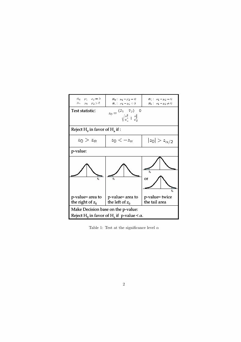
3. Test at the significance level α. (Table 1.)

¤£

¡¢EXAMPLE 6.1

A survey of credit card holders revealed that Americans carried an averagecredit card balance of $3900 in 1995 and $3300 in 1994 (U.S. News & WorldReport, January 1, 1996). Suppose that these averages are based on randomsamples of 400 credit card holders in 1995 and 450 credit card holders in 1994and that the sample standard deviations of the balances were $880 in 1995 and$810 in 1994.

(a) What is the point estimate of µ1 − µ2?

1

������������������ ���������������� �������������������������������

�

��������� ����� ��� ��������

�������������� � ������ �����

�������������� � ����� � �����

��������

����� �������������������

!� � � � ��:

������������������ ���������������� �������������������������������

�

��������� ����� ��� ��������

�������������� � ������ �����

�������������� � ����� � �����

��������

����� �������������������

!� � � � ��:

z0z0z0z0

z0z0

z0z0

Table 1: Test at the significance level α

2

(b) Construct a 95% confidence interval for the difference between the meancredit card balances for all credit card holders in 1995 and 1994.

(c) Test at the 1% significance level if the mean credit card balances for allcredit card holders in America in 1995 and 1994 were different.

(d) Please report the p-value of the above test. Based on this p-value, whatis your decision if

(1) the significance level is 0.01

(2) the significance level is 0.05

SOLUTION Refer to all credit card holders in 1995 as population 1 andall credit card holders in 1994 as population 2. The respective samples, then, aresamples 1 and 2. Let µ1 and µ2 be the mean credit card balances for populations1 and 2, and let x1 and x2 be the means of the respective samples. From thegiven information,

For 1995: n1 = 400, x1 = $3900, s1 = $880

For 1994: n2 = 450, x2 = $3300, s2 = $810

(a) The point estimate of µ1 − µ2 is given by the value of x1 − x2. Thus,

Point estimate of µ1 − µ2 = $3900− $3300 = $600

(b) The confidence level is 1− α = .95, so α = 0.05 and zα/2 = z0.025 = 1.96.

√s21

n1+

s22

n2=

√(880)2

400+

(810)2

450= $58.25804665

The 95% C.I. for (µ1 − µ2) is

(x1 − x2)± zα/2 ·√

s21

n1+

s22

n2= (3900− 3300)± 1.96 (58.25804665)

= 600± 114.19 = $485.81 to $714.19

Thus, with 95% confidence we can state that the difference in the meancredit card balances for all credit card holders in 1995 and 1994 was be-tween $485.81 and $714.19.

(c)

Step 1. State the null and alternative hypothesesWe are to test if the two population means are different. The twopossibilities are

3

(i) The mean credit card balances for all credit card holders in Amer-ica in 1995 and 1994 are not different. In other words, µ1 = µ2,which can be written as µ1 − µ2 = 0.

(ii) The mean credit card balances for all credit card holders in Amer-ica in 1995 and 1994 are different. That is, µ1 6= µ2, which canbe written as µ1 − µ2 6= 0.

Considering these two possibilities, the null and alternative hypothe-ses are

H0 : µ1 − µ2 = 0 (the two population means are not different)H1 : µ1 − µ2 6= 0 (the two population means are different)

Step 2. Select the distribution to useBecause n1 > 30 and n2 > 30, both sample sizes are large. Therefore,the sampling distribution of x1− x2 is approximately normal, and weuse the normal distribution to make the hypothesis test.

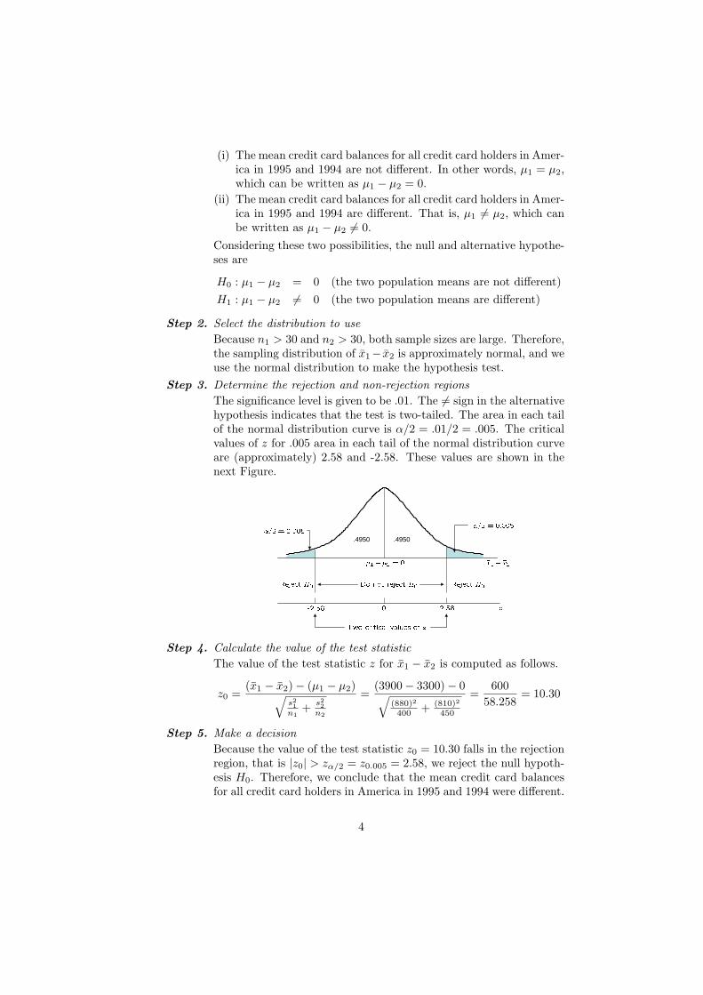
Step 3. Determine the rejection and non-rejection regionsThe significance level is given to be .01. The 6= sign in the alternativehypothesis indicates that the test is two-tailed. The area in each tailof the normal distribution curve is α/2 = .01/2 = .005. The criticalvalues of z for .005 area in each tail of the normal distribution curveare (approximately) 2.58 and -2.58. These values are shown in thenext Figure.

.4950 .4950

Step 4. Calculate the value of the test statisticThe value of the test statistic z for x1 − x2 is computed as follows.

z0 =(x1 − x2)− (µ1 − µ2)√

s21

n1+ s2

2n2

=(3900− 3300)− 0√

(880)2

400 + (810)2

450

=600

58.258= 10.30

Step 5. Make a decisionBecause the value of the test statistic z0 = 10.30 falls in the rejectionregion, that is |z0| > zα/2 = z0.005 = 2.58, we reject the null hypoth-esis H0. Therefore, we conclude that the mean credit card balancesfor all credit card holders in America in 1995 and 1994 were different.

4

(d) p-value is twice the tail area.

p− value = 2 · P (z > |z0|) = 2 · P (z > 10.30) ≈ 0

(1) Since p-value is less than 0.01, we can reject H0 at the significancelevel α = 0.01.

(2) Since p-value is less than 0.05, we can reject H0 at the significancelevel α = 0.05.

2. Two Independent Samples (sizes do not matter):

*Assumptions:

1. Both populations are normal.

2. The population variances are equal (σ21 = σ2

2), although unknown.

¨§

¥¦Key formulas

• Data

Sample 1: n1, X1, s21

Sample 2: n2, X2, s22

1. Point estimator of µ1 − µ2 : X1 − X2.

2. 100(1− α)% C.I. for µ1 − µ2 : X1 − X2 ± tdf,α/2sp

√1

n1+ 1

n2where

sp =

√(n1 − 1)s2

1 + (n2 − 1)s22

n1 + n2 − 2and df = n1 + n2 − 2

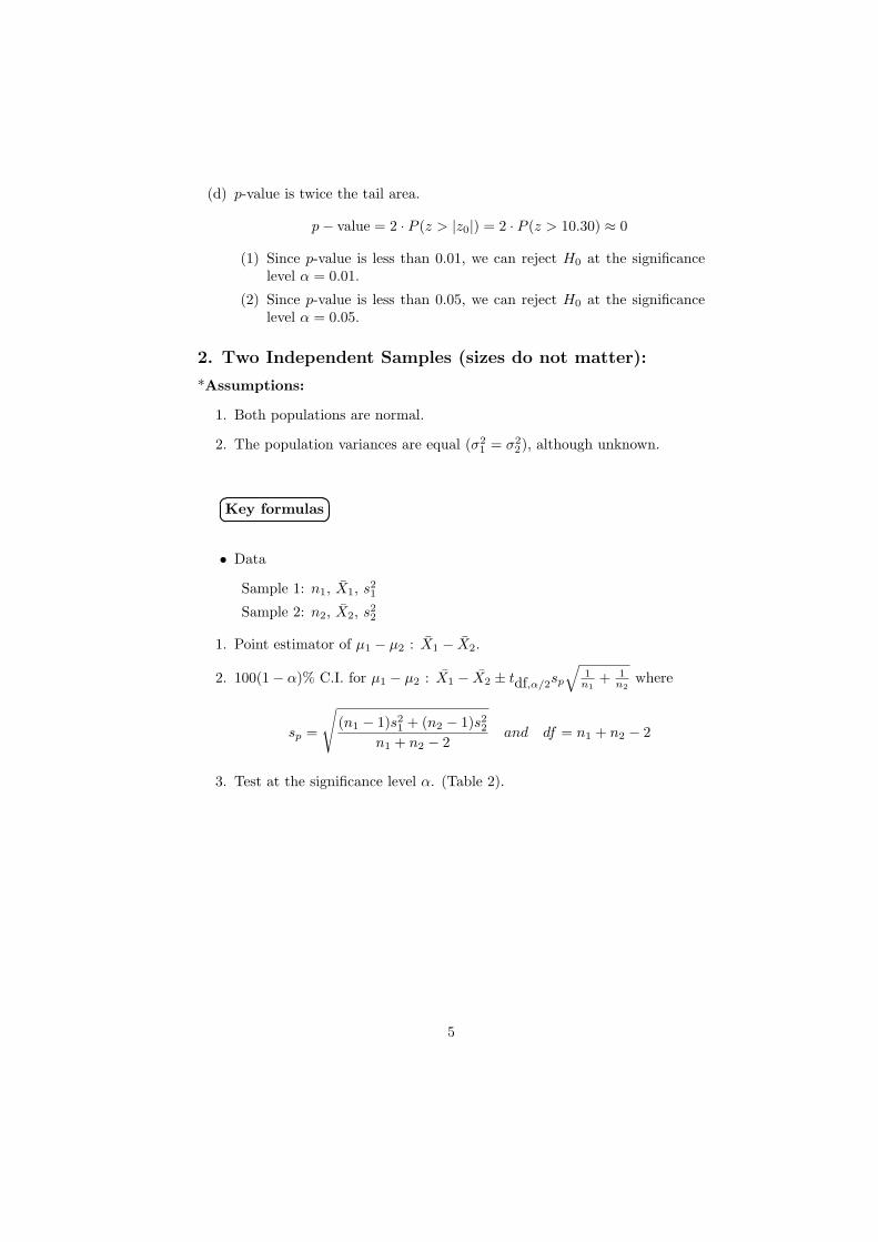
3. Test at the significance level α. (Table 2).

5

������������������ ���������������� �������������������������������

�

��������� ����� ��� ��������

�������������� � ������ ��� �

�������������� � ������� ��� �

��������

����� �������������������

� � � � ��:

������������������ ���������������� �������������������������������

�

��������� ����� ��� ��������

�������������� � ������ ��� �

�������������� � ������� ��� �

��������

����� �������������������

� � � � ��:

t0t0t0

t0t0

t0t0

Table 2: Test at the significance level α.

¨§

¥¦s2

p, a weighted average

The quantity sp in the confidence interval is an estimate of the common standard

deviation σ for the two populations and is formed by combining (pooling) information

from the two samples. In fact, s2p is a weighted average of the sample variances s2

1

and s22. For the special case where the sample sizes are the same (n1 = n2), the formula

for s2p reduces to s2

p = (s21 + s2

2)/2, the mean of the two sample variances. The degrees

of freedom for the confidence interval are a combination of the degrees of freedom for

the two samples; that is, df = (n1 − 1) + (n2 − 1) = n1 + n2 − 2. Recall that we

are assuming that the two populations from which we draw the samples have normal

distributions with a common variance σ2. If the confidence interval presented were

valid only when these assumptions were met exactly, the estimation procedure would

be of limited use. Fortunately, the confidence coefficient remains relatively stable if

both distributions are mound-shaped and the sample sizes are approximately equal.

More discussion about these assumptions is presented at the end of this section.

6

¤£

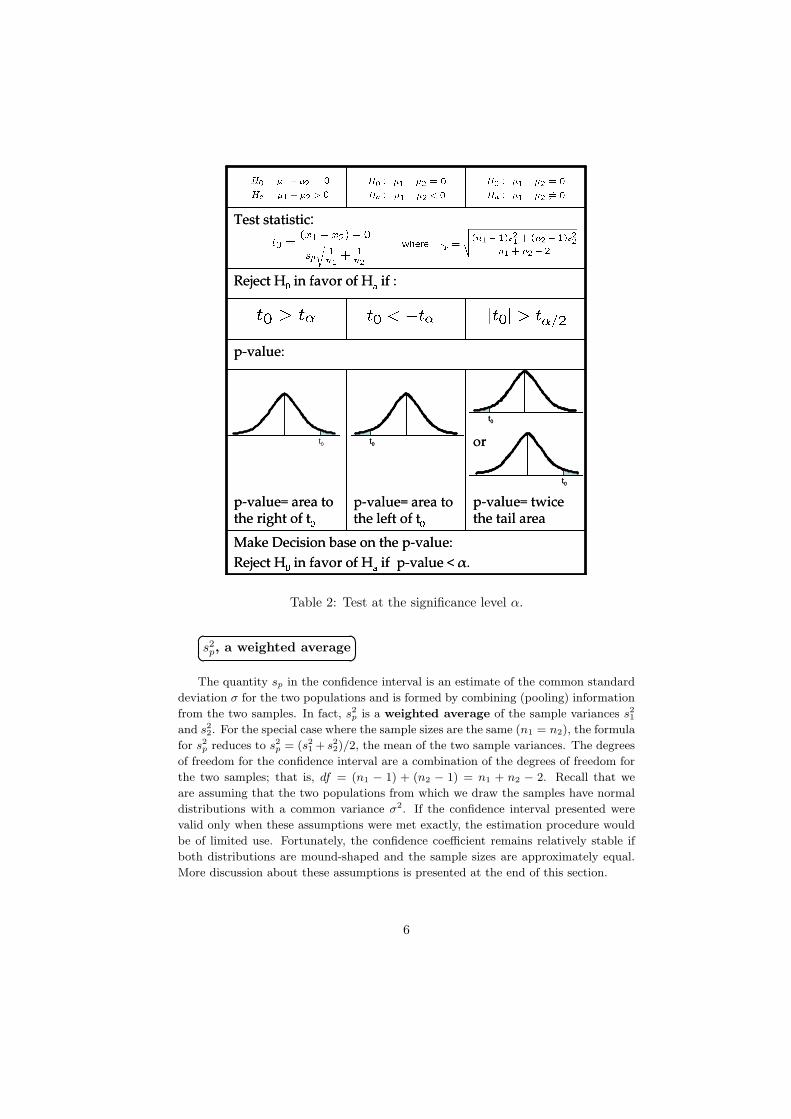
¡¢EXAMPLE 6.2

Company officials were concerned about the length of time a particular drugproduct retained its potency. A random sample, sample 1, of n1 = 10 bottlesof the product was drawn from the production line and analyzed for potency.

A second sample, sample 2, of n2 = 10 bottles was obtained and stored in aregulated environment for a period of one year.

The readings obtained from each sample are given in Table 3.Suppose we let µ1 denote the mean potency for all bottles that might be

sampled coming off the production line and µ2 denote the mean potency for allbottles that may be retained for a period of one year. Estimate µ1−µ2 by usinga 95% confidence interval.

Sample 1 Sample 2

∑j y1j = 103.7

∑j y2j = 98.3

∑j y2

1j = 1076.31∑

j y22j = 966.81

Then

y1 =103.710

= 10.37 y2 =98.310

= 9.83

s21 =

19

[1076.31− (103.7)2

10

]= .105 s2

2 =19

[966.81− (98.3)2

10

]= .058.

The estimate of the common standard deviation σ is

sp =

√(n1 − 1)s2

1 + (n2 − 1)s22

n1 + n2 − 2=

√9(.105) + 9(.058)

18= .285.

The t-value based on df = n1 + n2− 2 = 18 and α = .025 is t18,0.025 = 2.101. A95% confidence interval for the difference in mean potencies is

(10.37−9.83)±2.101(.285)√

1/10 + 1/10 or .54±.268. That is, (0.272, 0.808).

Sample 1 Sample 210.2 10.6 9.8 9.710.5 10.7 9.6 9.510.3 10.2 10.1 9.610.8 10.0 10.2 9.89.8 10.6 10.1 9.9

Table 3: Potency Reading for Two Samples

7

Therefore, we are 95% sure that the difference in mean potencies for the bottlesfrom the production line and those stored for 1 year, µ1−µ2, lies in the interval.272 to .808.

¤£

¡¢EXAMPLE 6.3

A study was conducted to determined whether persons in suburban district1 have a different mean income from those in district 2. A random sample of 20homeowners was taken in district 1. Although 20 homeowners were to be inter-viewed in district 2 also, 1 person refused to provide the information requested,even though the researcher promised to keep the interview confidential. So only19 observations were obtained from district 2. The data, recorded in thousandsof dollars, produced sample means and variances as shown in the following table.Use these data to construct a 95% confidence interval for (µ1 − µ2).

District 1 District 2Sample size 20 19Sample mean 18.27 16.78Sample variance 8.74 6.58

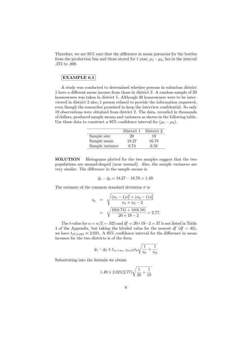
SOLUTION Histograms plotted for the two samples suggest that the twopopulations are mound-shaped (near normal). Also, the sample variances arevery similar. The difference in the sample means is

y1 − y2 = 18.27− 16.78 = 1.49.

The estimate of the common standard deviation σ is

sp =

√(n1 − 1)s2

1 + (n2 − 1)s22

n1 + n2 − 2

=

√19(8.74) + 18(6.58)

20 + 19− 2= 2.77.

The t-value for a = α/2 = .025 and df = 20+19−2 = 37 is not listed in Table4 of the Appendix, but taking the labeled value for the nearest df (df = 40),we have t37,0.025 ≈ 2.021. A 95% confidence interval for the difference in meanincomes for the two districts is of the form

y1 − y2 ± tn1+n2−2,α/2sp

√1n1

+1n2

Substituting into the formula we obtain

1.49± 2.021(2.77)

√120

+119

8

or1.49± 1.79.

Thus, we estimate the difference in mean incomes to lie somewhere in the intervalfrom −.30 to 3.28. If we multiply these limits by $1,000, the confidence intervalfor the difference in mean incomes is−$300 to $3,280. Since this interval includesboth positive and negative values for µ1 − µ2. We are unable to determinewhether the mean income for district 1 is larger or smaller than the meanincome for district 2. ♣

We can also test a hypothesis about the difference between two populationmeans. As with any test procedure, we begin by specifying a research hypothesisfor the difference in population means. Thus, we might, for example, specifythat the difference µ1 − µ2 is greater than some value D0. (Note: D0 will oftenbe 0.) The entire test procedure is summarized here, again.

¨§

¥¦A statistical Test for µ1 − µ2, Independent Samples

*Assumptions:

1. Both populations are normal.

2. The population variances are equal (σ21 = σ2

2), although unknown.

H0: µ1 − µ2 = D0 (D0 is specified)

Ha:

1. µ1 − µ2 > D0

2. µ1 − µ2 < D0

3. µ1 − µ2 6= D0

T.S. :t0 =

y1 − y2 −D0

sp

√1/n1 + 1/n2

R.R. : For a Type I error α and df = n1 + n2 − 2

1. reject H0 if t0 > tα

2. reject H0 if t0 < −tα

3. reject H0 if |t0| > tα/2

9

¤£

¡¢EXAMPLE 6.4

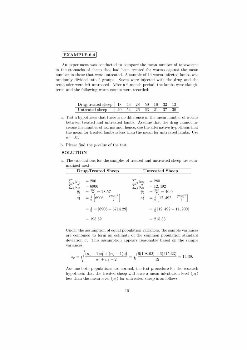
An experiment was conducted to compare the mean number of tapewormsin the stomachs of sheep that had been treated for worms against the meannumber in those that were untreated. A sample of 14 worm-infected lambs wasrandomly divided into 2 groups. Seven were injected with the drug and theremainder were left untreated. After a 6-month period, the lambs were slaugh-tered and the following worm counts were recorded:

Drug-treated sheep 18 43 28 50 16 32 13Untreated sheep 40 54 26 63 21 37 39

a. Test a hypothesis that there is no difference in the mean number of wormsbetween treated and untreated lambs. Assume that the drug cannot in-crease the number of worms and, hence, use the alternative hypothesis thatthe mean for treated lambs is less than the mean for untreated lambs. Useα = .05.

b. Please find the p-value of the test.

SOLUTION

a. The calculations for the samples of treated and untreated sheep are sum-marized next.

Drug-Treated Sheep Untreated Sheep

∑j y1j = 200

∑j y2j = 280∑

j y21j = 6906

∑j y2

2j = 12, 492y1 = 200

7 = 28.57 y2 = 2807 = 40.0

s21 = 1

6

[6906− (200)2

7

]s22 = 1

6

[12, 492− (280)2

7

]

= 16 = [6906− 5714.29] = 1

6 [12, 492− 11, 200]

= 198.62 = 215.33

Under the assumption of equal population variances, the sample variancesare combined to form an estimate of the common population standarddeviation σ. This assumption appears reasonable based on the samplevariances.

sp =

√(n1 − 1)s2

1 + (n2 − 1)s22

n1 + n2 − 2=

√6(198.62) + 6(215.33)

12= 14.39.

Assume both populations are normal, the test procedure for the researchhypothesis that the treated sheep will have a mean infestation level (µ1)less than the mean level (µ2) for untreated sheep is as follows.

10

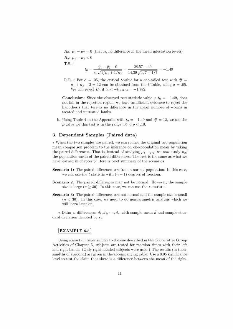
H0: µ1 − µ2 = 0 (that is, no difference in the mean infestation levels)

Ha: µ1 − µ2 < 0

T.S. :t0 =

y1 − y2 − 0sp

√1/n1 + 1/n2

=28.57− 40

14.39√

1/7 + 1/7= −1.49

R.R. : For α = .05, the critical t-value for a one-tailed test with df =n1 + n2 − 2 = 12 can be obtained from the t-Table, using a = .05.We will reject H0 if t0 < −t12,0.05 = −1.782.

Conclusion: Since the observed test statistic value is t0 = −1.49, doesnot fall in the rejection region, we have insufficient evidence to reject thehypothesis that tere is no difference in the mean number of worms intreated and untreated lambs.

b. Using Table 4 in the Appendix with t0 = −1.49 and df = 12, we see thep-value for this test is in the range .05 < p < .10.

3. Dependent Samples (Paired data)

∗ When the two samples are paired, we can reduce the original two-populationmean comparison problem to the inference on one-population mean by takingthe paired differences. That is, instead of studying µ1 − µ2, we now study µd,the population mean of the paired differences. The rest is the same as what wehave learned in chapter 5. Here is brief summary of the scenarios.

Scenario 1: The paired differences are from a normal population. In this case,we can use the t-statistic with (n− 1) degrees of freedom.

Scenario 2: The paired differences may not be normal. However, the samplesize is large (n ≥ 30). In this case, we can use the z-statistic.

Scenario 3: The paired differences are not normal and the sample size is small(n < 30). In this case, we need to do nonparametric analysis which wewill learn later on.

∗ Data: n differences: d1, d2, · · · , dn with sample mean d and sample stan-dard deviation denoted by sd.

¤£

¡¢EXAMPLE 6.5

Using a reaction timer similar to the one described in the Cooperative GroupActivities of Chapter 5, subjects are tested for reaction times with their leftand right hands. (Only right-handed subjects were used.) The results (in thou-sandths of a second) are given in the accompanying table. Use a 0.05 significancelevel to test the claim that there is a difference between the mean of the right-

11

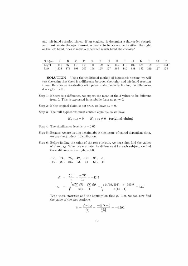
and left-hand reaction times. If an engineer is designing a fighter-jet cockpitand must locate the ejection-seat activator to be accessible to either the rightor the left hand, does it make a difference which hand she chooses?

Subject A B C D E F G H I J K L M N

Right 191 97 116 165 116 129 171 155 112 102 188 158 121 133

Left 224 171 191 207 196 165 177 165 140 188 155 219 177 174

SOLUTION Using the traditional method of hypothesis testing, we willtest the claim that there is a difference between the right- and left-hand reactiontimes. Because we are dealing with paired data, begin by finding the differencesd = right− left.

Step 1: If there is a difference, we expect the mean of the d values to be differentfrom 0. This is expressed in symbolic form as µd 6= 0.

Step 2: If the original claim is not true, we have µd = 0.

Step 3: The null hypothesis must contain equality, so we have

H0 : µd = 0 H1 : µd 6= 0 (original claim)

Step 4: The significance level is α = 0.05.

Step 5: Because we are testing a claim about the means of paired dependent data,we use the Student t distribution.

Step 6: Before finding the value of the test statistic, we must first find the valuesof d and sd. When we evaluate the difference d for each subject, we findthese differences d = right− left:

-33, -74, -75, -42, -80, -36, -6,-10, -28, -86, 33, -61, -56, -41

d =∑

d

n=−59514

= −42.5

sd =

√n(

∑d2)− (

∑d)2

n(n− 1)=

√14(39, 593)− (−595)2

14(14− 1)= 33.2

With these statistics and the assumption that µd = 0, we can now findthe value of the test statistic.

t0 =d− µd

sd√n

=−42.5− 0

33.2√14

= −4.790.

12

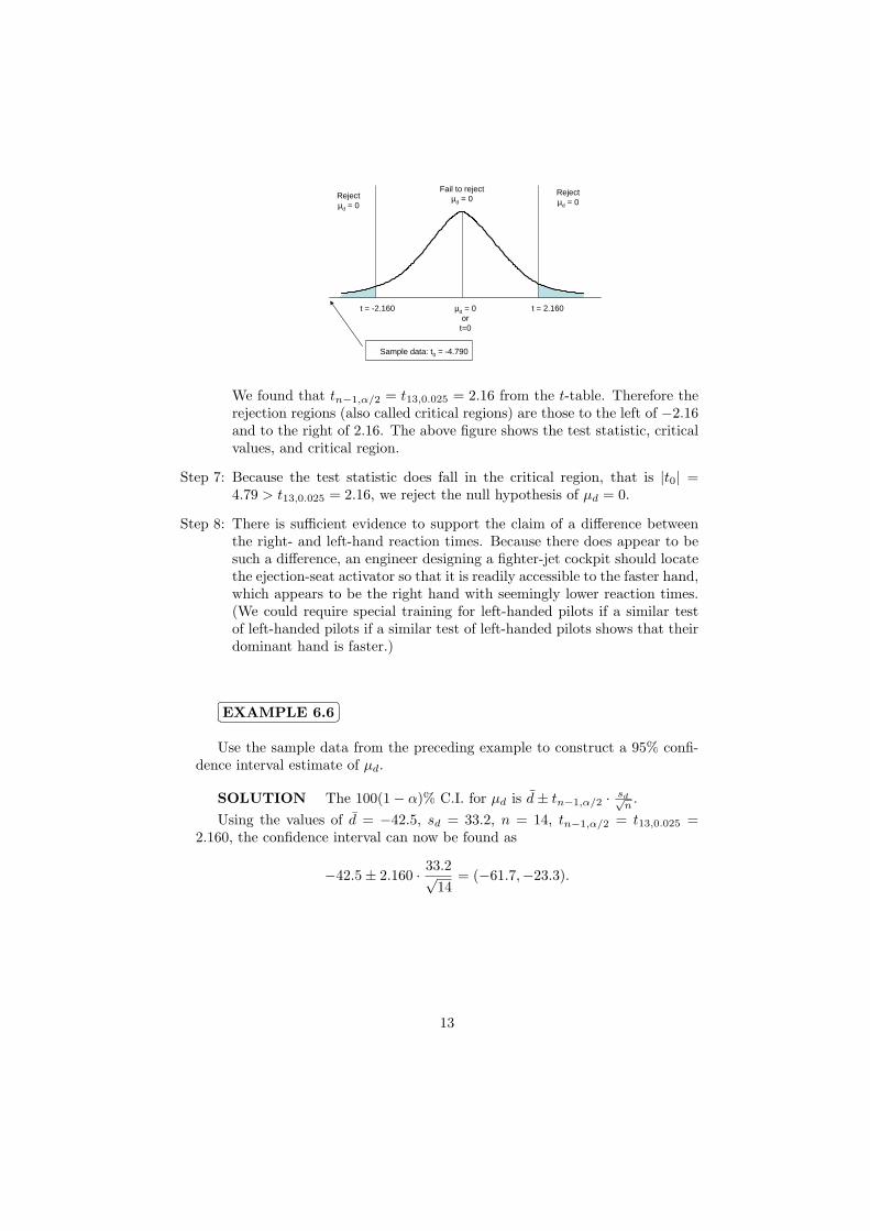
Fail to rejectµd = 0

Rejectµd = 0

Rejectµd = 0

µd = 0ort=0

t = 2.160t = -2.160

Sample data: t0 = -4.790

We found that tn−1,α/2 = t13,0.025 = 2.16 from the t-table. Therefore therejection regions (also called critical regions) are those to the left of −2.16and to the right of 2.16. The above figure shows the test statistic, criticalvalues, and critical region.

Step 7: Because the test statistic does fall in the critical region, that is |t0| =4.79 > t13,0.025 = 2.16, we reject the null hypothesis of µd = 0.

Step 8: There is sufficient evidence to support the claim of a difference betweenthe right- and left-hand reaction times. Because there does appear to besuch a difference, an engineer designing a fighter-jet cockpit should locatethe ejection-seat activator so that it is readily accessible to the faster hand,which appears to be the right hand with seemingly lower reaction times.(We could require special training for left-handed pilots if a similar testof left-handed pilots if a similar test of left-handed pilots shows that theirdominant hand is faster.)

¤£

¡¢EXAMPLE 6.6

Use the sample data from the preceding example to construct a 95% confi-dence interval estimate of µd.

SOLUTION The 100(1− α)% C.I. for µd is d± tn−1,α/2 · sd√n.

Using the values of d = −42.5, sd = 33.2, n = 14, tn−1,α/2 = t13,0.025 =2.160, the confidence interval can now be found as

−42.5± 2.160 · 33.2√14

= (−61.7,−23.3).

13

¨§

¥¦Crest and Dependent Samples

In the late 1950s, Procter & Gamble introduced Crest toothpasteas the first such product with fluoride. To test the effectivenessof Crest in reducing cavities, researchers conducted experimentswith several sets of twins. One of the twins in each set was givenCrest with fluoride, while the other twin continued to use ordinarytoothpaste without fluoride. It was believed that each pair of twinswould have similar eating, brushing, and genetic characteristics.

Results showed that the twins who used Crest had significantly fewer cavities thanthose who did not. This use of twins as dependent samples allowed the researchersto control many of the different variables affecting cavities.

14

¨§

¥¦A Little Bit of History

¤£

¡¢Carl Friedrich Gauss

The normal probability distribution is often referred to as the Gaus-sian distribution in honor of Carl Gauss, the individual thought tohave discovered the idea. However, it was actually Abraham deMoivre who first wrote down the equation of the normal distribu-tion. Gauss was born in Brunswick, Germany, on April 30, 1777.Gauss’ mathematical prowess was evident early in his life. At ageeight he was able to instantly add the first 100 integers. In 1792,Gauss entered the Brunswick Collegium Corolinum and remained

there for three years. In 1795, Gauss entered the University of Gottingen. In 1799,Gauss earned his doctorate. The subject of his dissertation was the FundamentalTheorem of Algebra. In 1809, Gauss published a book on the mathematics of plane-tary orbits. In this book, he further developed the theory of least-squares regressionby analyzing the errors. The analysis of these errors led to the discovery that errorsfollow a normal distribution. Gauss was considered to be “glacially cold” as a personand had troubled relationships with his family. Gauss died February 23, 1855.

¤£

¡¢Abraham de Moivre

Abraham de Moivre was born in France on May 26, 1667. Heis known as a great contributor to the areas of probability andtrigonometry. De Moivre studied for five years at the Protestantacademy at Sedan. From 1682 to 1684, he studied logic at Saumur.In 1685, he moved to England. De Moivre was elected a fellow ofthe Royal Society in 1697. He was part of the commission to settlethe dispute between Newton and Leibniz regarding the discovererof calculus. He published The Doctrine of Chance in 1718. In1733, he developed the equation that describes the normal curve. Unfortunately,de Moivre had a difficult time being accepted in English society (perhaps due tohis accent) and was able to make only a meager living tutoring mathematics. Aninteresting piece of information regarding de Moivre; he correctly predicted the dayof his death, Nov. 27, 1754.

15

¨§

¥¦William Sealy Gossett

William Sealy Gossett was born on June 13, 1876, in Canterbury, Eng-

land. Gossett earned a degree in chemistry from New College in Oxford

in 1899. He then got a job as a chemist for the Guinness Brewing Com-

pany. Gossett, along with other chemists, was asked to find a way to

make the best beer at the cheapest cost. This allowed him to concen-

trate on statistics. In 1904, Gossett wrote a paper on the brewing of

beer that included a discussion of standard errors. In July, 1905, Gossett

met with Karl Pearson to learn about the theory of standard errors. Over

the next few years, he developed his t-distribution. The Guinness Brewery did not allow

its employees to publish, so Gossett published his research using the pen name Student.

Gossett died October 16, 1937.

16

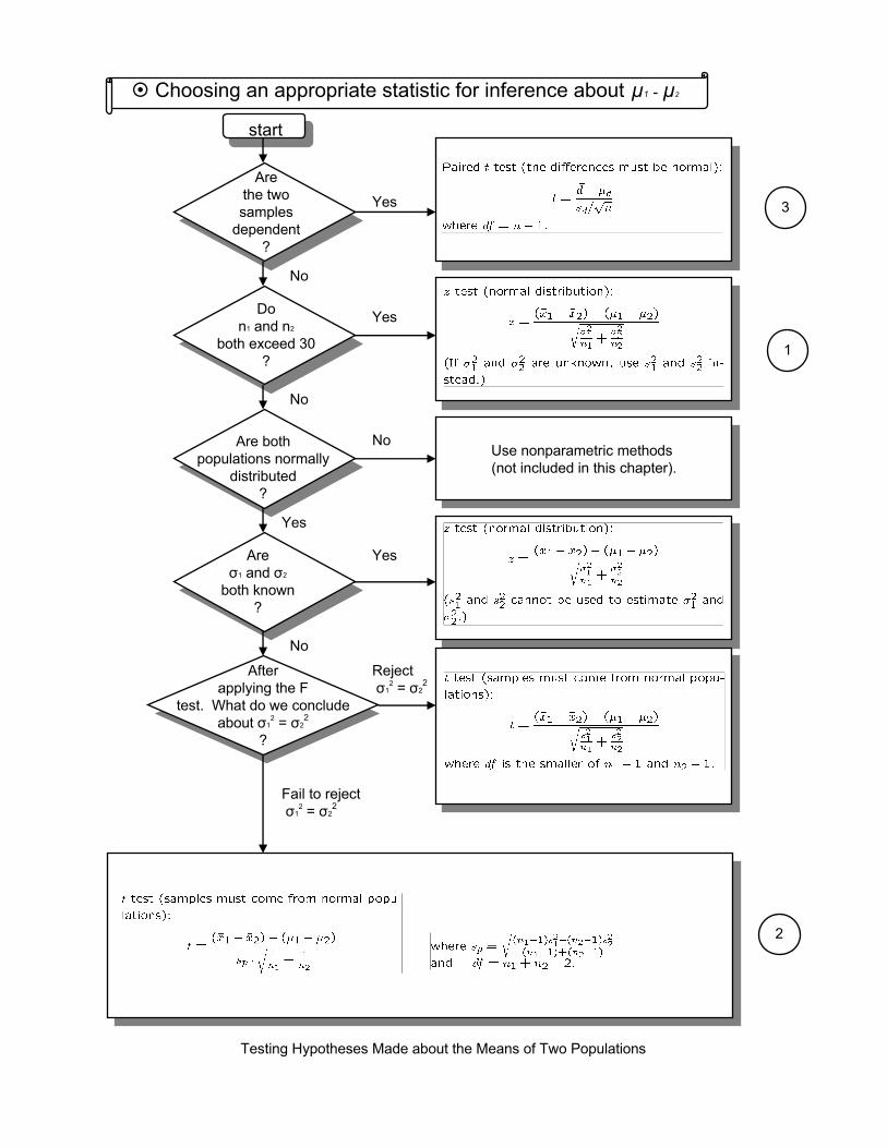
Use nonparametric methods (not included in this chapter).

start

Arethe twosamples

dependent?

Don1 and n2

both exceed 30?

Are bothpopulations normally

distributed?

Areσ1 and σ2

both known?

Afterapplying the F

test. What do we concludeabout σ1

2 = σ22

?

Yes

Yes

Yes

No

Yes

No

No

No

Rejectσ1

2 = σ22

Fail to rejectσ1

2 = σ22

Testing Hypotheses Made about the Means of Two Populations

3

1

2

Choosing an appropriate statistic for inference about µ1 - µ2

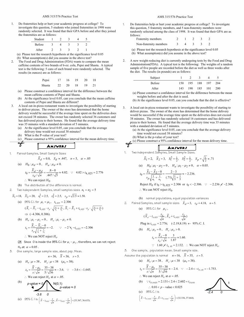
AMS 315/576 Practice Test

1. Do fraternities help or hurt your academic progress at college? To investigate this question, 5 students who joined fraternities in 1998 were randomly selected. It was found that their GPA before and after they joined the fraternities are as follows:

Student 1 2 3 4 5

Before 3 4 3 3 2 After 2 3 3 2 1

(a) Please test the research hypothesis at the significance level 0.05 (b) What assumption(s) did you assume in the above test?

2. The Food and Drug Administration (FDA) wants to compare the mean caffeine contents of two brands of 6-oz. cola, Pepsi and Shasta. A typical test is the following: 5 cans of each brand were randomly selected. The results (in ounces) are as follows:

(a) Please construct a confidence interval for the difference between the

mean caffeine contents of Pepsi and Shasta. (b) At the significance level 0.05, can you conclude that the mean caffeine

contents of Pepsi and Shasta are different? 3. A local eat-in-pizza restaurant wants to investigate the possibility of starting

to deliver pizzas. The owner of the store has determined that the home delivery would be successful if the average time spent on the deliveries does not exceed 38 minutes. The owner has randomly selected 36 customers and has delivered pizza to their homes. He found that the average delivery time was 35 minutes with a standard deviation of 5 minutes. (a) At the significance level 0.05, can you conclude that the average

delivery time would not exceed 38 minutes? (b) What is the P-value of your test? (c) Please construct a 95% confidence interval for the mean delivery time.

1. Paired-Samples, Small Sample Sizes

0.8, .447, 5, .05d dX S n α= ≈ = =

(a) 0 : 0 , : 0.d a dH Hµ µ= ≠

0 4,.025

0

.8 0 4.02. 4.02 2.776/ .447 / 5

We can reject .

d d

d

Xt t

s nH

µ− −= = ≈ > =

∴

∵

(b) The distribution of the difference is normal. 2. Two independent Samples, small samples sizes 1 2 5n n= =

2 21 2 1 218, 20, 2.5, 2.5, 2.5 1.58.pX X s s s= = = = = ≈

(a) 95% C.I. for 1 2 8,.025, 2.306tµ µ= =

1 2 1 2

1 1 1 11 2 8,.025 1 2 8,.025( , )

( 4.306, 0.306).p pn n n nX X t s X X t s− − ⋅ ⋅ + − + ⋅ ⋅ +

⇒ −

(b) 0 1 2 1 2: 0 , : 0.aH Hµ µ µ µ− = − ≠

1 2

1 20 8,.0251 1

0

0 2. 2 2.306

We can NOT reject .p n n

X Xt ts

H

− −= = − − < − = −

+

∴

∵

OR Since 0 is inside the 95% C.I. for 1 2µ µ− , therefore, we can not reject

H0 at 0.05α = . 3. One sample, large sample size, about pop. Mean.

36, 36, 5.n X s= = =

(a) 0 0: 38 , : 38 ( 38).aH Hµ µ µ= < =

00

0

35 38 3.6. 3.6 1.645./ 5 / 36

We can reject at .05.

Xzs n

H

µ

α

− −= = ≈ − − < −

∴ =

∵

(b)

(c) 95% C. I is

0.025 0.025, (33.367, 36.633).s sX z X zn n

− ⋅ + ⋅ =

AMS 315/576 Practice Test

1. Do fraternities help or hurt your academic progress at college? To investigate this question, 5 fraternity members, and 5 non-fraternity members were randomly selected among the class of 1998. It was found that their GPA are as follows:

Fraternity members 2 1 2 3 2 Non-fraternity members 3 4 3 3 2

(a) Please test the research hypothesis at the significance level 0.05 (b) What assumption(s) did you assume in the above test?

2. A new weight-reducing diet is currently undergoing tests by the Food and Drug Administration(FDA). A typical test is the following: The weights of a random sample of five people are recorded before the diet as well as three weeks after the diet. The results (in pounds) are as follows:

(a) Please construct a confidence interval for the difference between the mean weights before and after the diet is used.

(b) At the significance level 0.05, can you conclude that the diet is effective?

3. A local eat-in-pizza restaurant wants to investigate the possibility of starting to deliver pizzas. The owner of the store has determined that the home delivery would be successful if the average time spent on the deliveries does not exceed 38 minutes. The owner has randomly selected 16 customers and has delivered pizza to their homes. He found that the average delivery time was 35 minutes with a standard deviation of 5 minutes.

(a) At the significance level 0.05, can you conclude that the average delivery time would not exceed 38 minutes?

(b) What is the p-value of your test? (c) Please construct a 95% confidence interval for the mean delivery time.

1. Two independent Samples, Small Sample Sizes.

2 21 1 11 2 1 22 2 22, 3, , , .71pX X S S S= = = = = ≈

(a) 0 1 2 1 2: 0 , : 0, 0.05.aH Hµ µ µ µ α− = − ≠ =

1 2

1 20 1 1 1 1

5 5

0 0 8,.025 0

0

0 2 3 2.236.(.71)

Reject if 2.306 or 2.306. 2.236 2.306.

We can NOT reject .

p n n

X Xts

H t t t

H

− − −= = ≈ −

+ +

> = < − − < −

∴

∵

(b) normal populations, equal population variances

2. Paired Samples, small sample sizes 3, 4.18, 5.d dX s n= =

(a) 95% C.I. for ,dµ

4,.025 4,.025

4,.025

( , )

Plug in 2.776; (-2.19,8.19) 95% C. I.

d dd d

s sX t X tn n

t

− ⋅ + ⋅

= ←

(b) 0 : 0 , : 0.d a dH Hµ µ= >

0

4, .05 0

0 3 1.60.1.87/

1.60 2.132. We can NOT reject .

d

d

Xts n

t H

−= = ≈

> = ∴∵

3. One sample, population mean. Small sample size. Assume the population is normal 16, 35, 5.n X s= = =

(a) 0 0: 38 , : 38 ( 38).aH Hµ µ µ= < =

00 15, .05

0

35 38 2.4. 2.4 1.753./ 5 / 16

We can reject at .05.

Xt ts n

H

µ

α

− −= = ≈ − − < − = −

∴ =

∵

(b) 15,0.025 15,0.012.131 2.4 2.602t t= < < =∵

0.01 value 0.025p∴ < − < (c) 95% C. I is

15, 0.025 15, 0.025, (32.336, 37.664).s sX t X tn n

− ⋅ + ⋅ =

Pepsi 17 16 19 20 18

Shasta 22 20 18 19 21

Subject 1 2 3 4 5

Before 150 195 188 197 204 After 143 190 185 101 200

Answers Answers

p-value ≈ 0

-3.6 0

N(0,1) p-value ≈ 0

0

t

-2.4