![MEDILIG SQL v1 · Page 7 of 49 [MEDILIG SQL V1.0] 9 Σεʍʑεμβʎίοʒ 2010 Schema Notation This is a brief navigational guide to the notation we used to design the Clinica and](https://static.fdocument.org/doc/165x107/60bafb42b1f28906cf51d084/medilig-sql-v1-page-7-of-49-medilig-sql-v10-9-2010-schema.jpg)
Algorithmns and...
48
Algorithmns and Datastructures O-Notation, L’Hopital Albert-Ludwigs-Universität Freiburg Prof. Dr. Rolf Backofen Bioinformatics Group / Department of Computer Science Algorithmns and Datastructures, November 2018
Transcript of Algorithmns and...
Algorithmns and DatastructuresO-Notation, L’Hopital
Albert-Ludwigs-Universität Freiburg
Prof. Dr. Rolf BackofenBioinformatics Group / Department of Computer ScienceAlgorithmns and Datastructures, November 2018
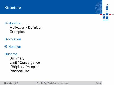
Structure
O-NotationMotivation / DefinitionExamples
Ω-Notation
Θ-Notation
RuntimeSummaryLimit / ConvergenceL’Hôpital / l’HospitalPractical use
November 2018 Prof. Dr. Rolf Backofen – beamer-ufcd 2 / 56
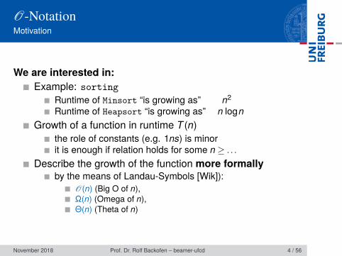
O-NotationMotivation
We are interested in:Example: sorting
Runtime of Minsort “is growing as” n2
Runtime of Heapsort “is growing as” n lognGrowth of a function in runtime T (n)
the role of constants (e.g. 1ns) is minorit is enough if relation holds for some n≥ . . .
Describe the growth of the function more formallyby the means of Landau-Symbols [Wik]):
O(n) (Big O of n),Ω(n) (Omega of n),Θ(n) (Theta of n)
November 2018 Prof. Dr. Rolf Backofen – beamer-ufcd 4 / 56
O-NotationDefinition
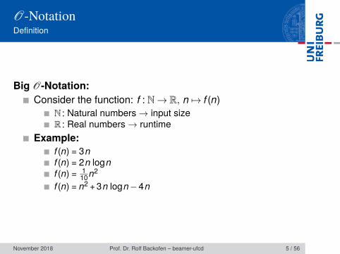
Big O-Notation:Consider the function: f : N→ R, n 7→ f (n)
N : Natural numbers→ input sizeR : Real numbers→ runtime
Example:f (n) = 3nf (n) = 2n lognf (n) = 1
10n2
f (n) = n2 +3n logn−4n
November 2018 Prof. Dr. Rolf Backofen – beamer-ufcd 5 / 56
O-NotationDefinition
Big O-Notation:Given two functions f and g:f ,g : N→ RIntuitive: f is Big-O of g (f is O(g))
. . . if f relative to g does not grow faster than gthe growth rate matters, not the absolute values
November 2018 Prof. Dr. Rolf Backofen – beamer-ufcd 6 / 56
O-NotationDefinition
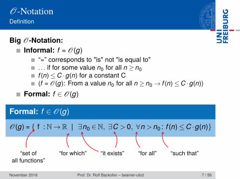
Big O-Notation:Informal: f = O(g)
“=” corresponds to "is" not "is equal to". . . if for some value n0 for all n≥ n0f (n)≤ C ·g(n) for a constant C(f = O(g): From a value n0 for all n≥ n0→ f (n)≤ C ·g(n))
Formal: f ∈ O(g)
Formal: f ∈ O(g)
O(g) = f : N→R | ∃n0 ∈N, ∃C > 0, ∀n > n0 : f (n)≤C ·g(n)
“set ofall functions”
“for which” “it exists” “for all” “such that”
November 2018 Prof. Dr. Rolf Backofen – beamer-ufcd 7 / 56
O-NotationExamples
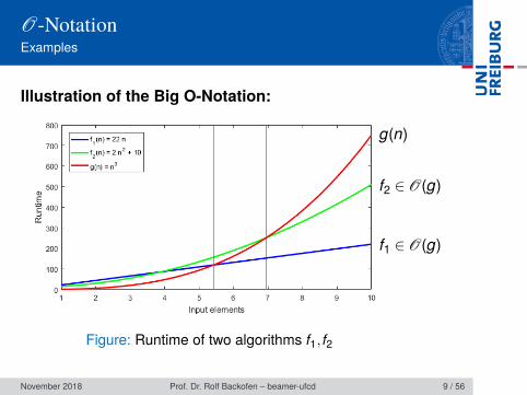
Illustration of the Big O-Notation:
Figure: Runtime of two algorithms f1, f2
g(n)
f2 ∈ O(g)
f1 ∈ O(g)
November 2018 Prof. Dr. Rolf Backofen – beamer-ufcd 9 / 56
O-NotationExamples
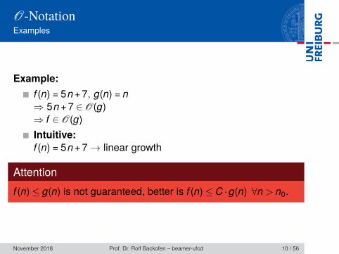
Example:f (n) = 5n +7, g(n) = n⇒ 5n +7 ∈ O(g)⇒ f ∈ O(g)Intuitive:f (n) = 5n +7→ linear growth
Attentionf (n)≤ g(n) is not guaranteed, better is f (n)≤ C ·g(n) ∀n > n0.
November 2018 Prof. Dr. Rolf Backofen – beamer-ufcd 10 / 56
O-NotationProof
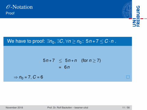
We have to proof: ∃n0, ∃C, ∀n≥ n0 : 5n +7≤ C ·n .
5n +7 ≤ 5n + n (for n≥ 7)= 6n
⇒ n0 = 7, C = 6
November 2018 Prof. Dr. Rolf Backofen – beamer-ufcd 11 / 56
O-NotationProof
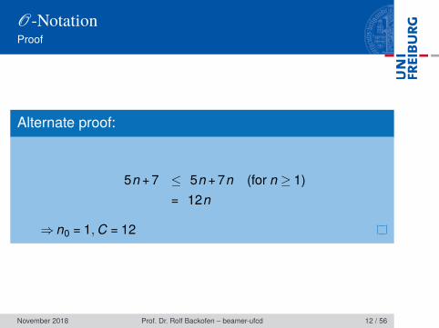
Alternate proof:
5n +7 ≤ 5n +7n (for n≥ 1)= 12n
⇒ n0 = 1, C = 12
November 2018 Prof. Dr. Rolf Backofen – beamer-ufcd 12 / 56
O-NotationExamples
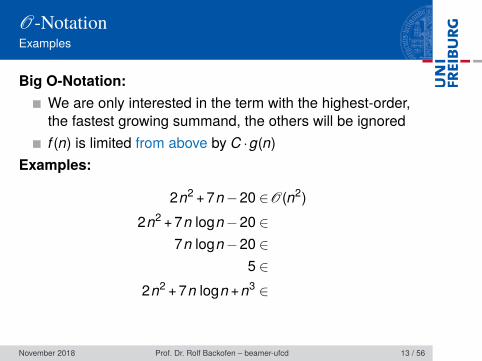
Big O-Notation:We are only interested in the term with the highest-order,the fastest growing summand, the others will be ignoredf (n) is limited from above by C ·g(n)
Examples:
2n2 +7n−20 ∈O(n2)2n2 +7n logn−20 ∈
7n logn−20 ∈5 ∈
2n2 +7n logn + n3 ∈
November 2018 Prof. Dr. Rolf Backofen – beamer-ufcd 13 / 56
O-NotationExamples
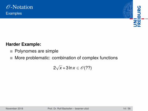
Harder Example:Polynomes are simpleMore problematic: combination of complex functions
2√
x +3lnx ∈ O(??)
November 2018 Prof. Dr. Rolf Backofen – beamer-ufcd 14 / 56
Ω-NotationDefinition
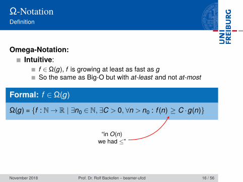
Omega-Notation:Intuitive:
f ∈Ω(g), f is growing at least as fast as gSo the same as Big-O but with at-least and not at-most
Formal: f ∈Ω(g)
Ω(g) = f : N→ R | ∃n0 ∈ N, ∃C > 0, ∀n > n0 : f (n) ≥ C ·g(n)
“in O(n)we had ≤”
November 2018 Prof. Dr. Rolf Backofen – beamer-ufcd 16 / 56
Ω-NotationProof
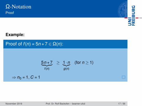
Example:
Proof of f (n) = 5n +7 ∈Ω(n):
5n +7︸ ︷︷ ︸f (n)
≥ 1 ·n︸︷︷︸g(n)
(for n≥ 1)
⇒ n0 = 1, C = 1
November 2018 Prof. Dr. Rolf Backofen – beamer-ufcd 17 / 56

Ω-NotationExamples
Illustration of the Omega-Notation:
Figure: Runtime of two algorithms f1, f2
f2 ∈Ω(g)
f1 ∈Ω(g)
g(n)
November 2018 Prof. Dr. Rolf Backofen – beamer-ufcd 18 / 56
Ω-NotationExamples
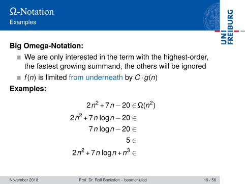
Big Omega-Notation:We are only interested in the term with the highest-order,the fastest growing summand, the others will be ignoredf (n) is limited from underneath by C ·g(n)
Examples:
2n2 +7n−20 ∈Ω(n2)2n2 +7n logn−20 ∈
7n logn−20 ∈5 ∈
2n2 +7n logn + n3 ∈
November 2018 Prof. Dr. Rolf Backofen – beamer-ufcd 19 / 56
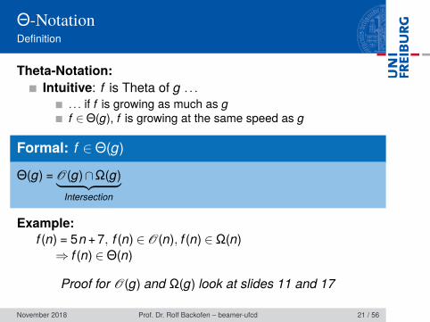
Θ-NotationDefinition
Theta-Notation:Intuitive: f is Theta of g . . .
. . . if f is growing as much as gf ∈Θ(g), f is growing at the same speed as g
Formal: f ∈Θ(g)
Θ(g) = O(g)∩Ω(g)︸ ︷︷ ︸Intersection
Example:f (n) = 5n +7, f (n) ∈ O(n), f (n) ∈Ω(n)⇒ f (n) ∈Θ(n)
Proof for O(g) and Ω(g) look at slides 11 and 17
November 2018 Prof. Dr. Rolf Backofen – beamer-ufcd 21 / 56
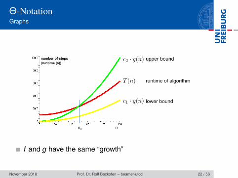
Θ-NotationGraphs
nn0
number of steps(runtime (s))
runtime of algorithm
upper bound
lower bound
f and g have the same “growth”
November 2018 Prof. Dr. Rolf Backofen – beamer-ufcd 22 / 56
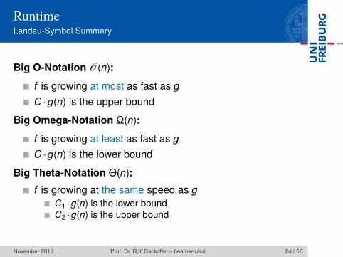
RuntimeLandau-Symbol Summary
Big O-Notation O(n):
f is growing at most as fast as gC ·g(n) is the upper bound
Big Omega-Notation Ω(n):
f is growing at least as fast as gC ·g(n) is the lower bound
Big Theta-Notation Θ(n):f is growing at the same speed as g
C1 ·g(n) is the lower boundC2 ·g(n) is the upper bound
November 2018 Prof. Dr. Rolf Backofen – beamer-ufcd 24 / 56
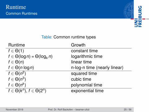
RuntimeCommon Runtimes
Table: Common runtime types
Runtime Growthf ∈Θ(1) constant timef ∈Θ(logn) = Θ(logk n) logarithmic timef ∈Θ(n) linear timef ∈Θ(n logn) n-log-n time (nearly linear)f ∈Θ(n2) squared timef ∈Θ(n3) cubic timef ∈Θ(nk) polynomial timef ∈Θ(kn), f ∈Θ(2n) exponential time
November 2018 Prof. Dr. Rolf Backofen – beamer-ufcd 25 / 56
So far discussed:Membership in O(. . .) proofed by hand:Explicit calculation of n0 and C
However: Both hint at limits in calculus
November 2018 Prof. Dr. Rolf Backofen – beamer-ufcd 27 / 56
O-NotationLimit / Convergence
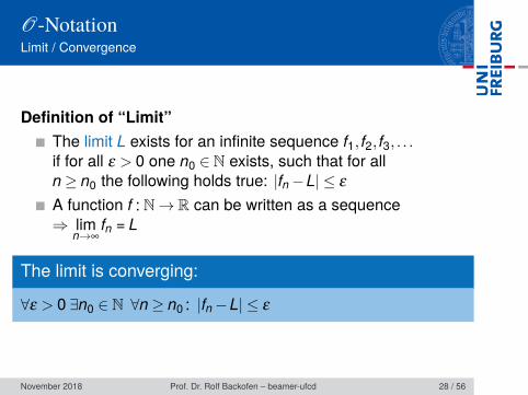
Definition of “Limit”The limit L exists for an infinite sequence f1, f2, f3, . . .if for all ε > 0 one n0 ∈ N exists, such that for alln≥ n0 the following holds true: |fn−L| ≤ ε
A function f : N→ R can be written as a sequence⇒ lim
n→∞fn = L
The limit is converging:
∀ε > 0 ∃n0 ∈ N ∀n≥ n0 : |fn−L| ≤ ε
November 2018 Prof. Dr. Rolf Backofen – beamer-ufcd 28 / 56
O-NotationLimit / Convergence
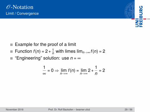
Example for the proof of a limitFunction f (n) = 2+ 1
n with limes limn→∞ f (n) = 2“Engineering” solution: use n = ∞
1∞
= 0⇒ limn→∞
f (n) = limn→∞
2+ 1n = 2
November 2018 Prof. Dr. Rolf Backofen – beamer-ufcd 29 / 56
O-NotationLimit / Convergence
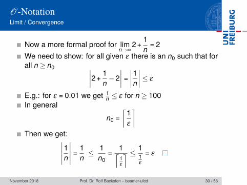
Now a more formal proof for limn→∞
2+ 1n = 2
We need to show: for all given ε there is an n0 such that forall n≥ n0 ∣∣∣∣2+ 1
n −2∣∣∣∣ =∣∣∣∣1n∣∣∣∣≤ ε
E.g.: for ε = 0.01 we get 1n ≤ ε for n≥ 100
In generaln0 =
⌈1ε
⌉Then we get:∣∣∣∣∣1n
∣∣∣∣∣ = 1n ≤
1n0
= 1⌈1ε
⌉ ≤ 11ε
= ε
November 2018 Prof. Dr. Rolf Backofen – beamer-ufcd 30 / 56
O-NotationLimit / Convergence
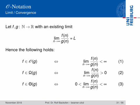
Let f ,g : N→ R with an existing limit
limn→∞
f (n)g(n) = L
Hence the following holds:
f ∈ O(g) ⇔ limn→∞
f (n)g(n) < ∞ (1)
f ∈Ω(g) ⇔ limn→∞
f (n)g(n) > 0 (2)
f ∈Θ(g) ⇔ 0< limn→∞
f (n)g(n) < ∞ (3)
November 2018 Prof. Dr. Rolf Backofen – beamer-ufcd 31 / 56
O-NotationLimit / Convergence
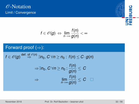
f ∈ O(g) ⇔ limn→∞
f (n)g(n) < ∞
Forward proof (⇒):
f ∈ O(g) def. of O(n)⇒ ∃n0, C ∀n≥ n0 : f (n)≤ C ·g(n)
⇒∃n0, C ∀n≥ n0 : f (n)g(n) ≤ C
⇒ limn→∞
f (n)g(n) ≤ C
November 2018 Prof. Dr. Rolf Backofen – beamer-ufcd 32 / 56
O-NotationLimit / Convergence
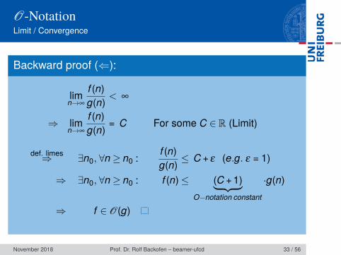
Backward proof (⇐):
limn→∞
f (n)g(n) < ∞
⇒ limn→∞
f (n)g(n) = C For some C ∈ R (Limit)
def. limes⇒ ∃n0, ∀n≥ n0 : f (n)g(n) ≤ C + ε (e.g. ε = 1)
⇒ ∃n0, ∀n≥ n0 : f (n)≤ (C +1)︸ ︷︷ ︸O−notation constant
·g(n)
⇒ f ∈ O(g)
November 2018 Prof. Dr. Rolf Backofen – beamer-ufcd 33 / 56
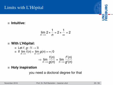
Limits with L’Hôpital
Intuitive:
limn→∞
2+ 1n = 2+ 1
∞= 2
With L’Hôpital:Let f , g : N→ RIf lim
n→∞f (n) = lim
n→∞g(n) = ∞/0
⇒ limn→∞
f (n)g(n) = lim
n→∞
f ′(n)g′(n)
Holy inspirationyou need a doctoral degree for that
November 2018 Prof. Dr. Rolf Backofen – beamer-ufcd 35 / 56
Limits with L’Hôpital
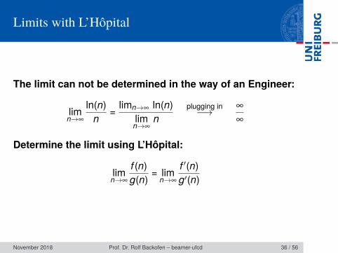
The limit can not be determined in the way of an Engineer:
limn→∞
ln(n)n = limn→∞ ln(n)
limn→∞
nplugging in−→ ∞
∞
Determine the limit using L’Hôpital:
limn→∞
f (n)g(n) = lim
n→∞
f ′(n)g′(n)
November 2018 Prof. Dr. Rolf Backofen – beamer-ufcd 36 / 56
Limits with L’Hôpital
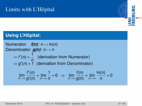
Using L’Hôpital:
Numerator: f(n) : n 7→ ln(n)Denominator: g(n) : n 7→ n⇒ f ′(n) = 1
n (derivation from Numerator)⇒ g′(n) = 1 (derivation from Denominator)
limn→∞
f ′(n)g′(n) = lim
n→∞
1n = 0 ⇒ lim
n→∞
f (n)g(n) = lim
n→∞
ln(n)n = 0
November 2018 Prof. Dr. Rolf Backofen – beamer-ufcd 37 / 56
Limits with L’Hôpital
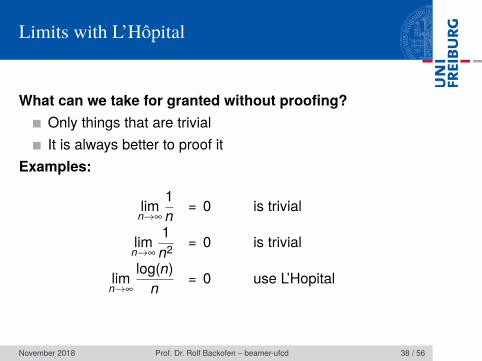
What can we take for granted without proofing?Only things that are trivialIt is always better to proof it
Examples:
limn→∞
1n = 0 is trivial
limn→∞
1n2 = 0 is trivial
limn→∞
log(n)n = 0 use L’Hopital
November 2018 Prof. Dr. Rolf Backofen – beamer-ufcd 38 / 56
O-NotationPractical use
Practical use:It is much easier to determine the runtime of an algorithmby using the O-Notation
1 Computing rules2 Practical use
November 2018 Prof. Dr. Rolf Backofen – beamer-ufcd 40 / 56
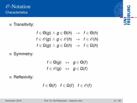
O-NotationCharacteristics
Transitivity:
f ∈Θ(g) ∧ g ∈Θ(h) → f ∈Θ(h)f ∈ O(g) ∧ g ∈ O(h) → f ∈ O(h)f ∈Ω(g) ∧ g ∈Ω(h) → f ∈Ω(h)
Symmetry:
f ∈Θ(g) ↔ g ∈Θ(f )f ∈ O(g) ↔ g ∈Ω(f )
Reflexivity:
f ∈Θ(f ) f ∈Ω(f ) f ∈ O(f )
November 2018 Prof. Dr. Rolf Backofen – beamer-ufcd 41 / 56
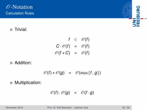
O-NotationCalculation Rules
Trivial:
f ∈ O(f )C ·O(f ) = O(f )O(f + C) = O(f )
Addition:
O(f ) + O(g) = O(maxf , g)
Multiplication:
O(f ) ·O(g) = O(f ·g)
November 2018 Prof. Dr. Rolf Backofen – beamer-ufcd 42 / 56
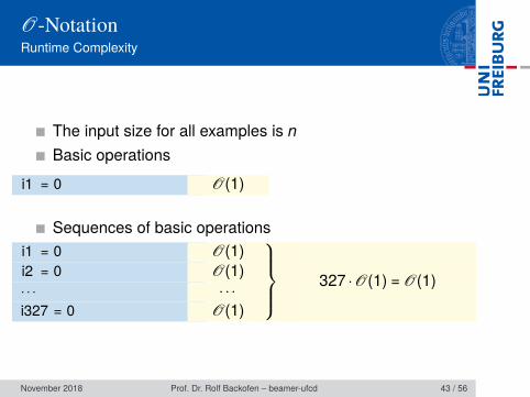
O-NotationRuntime Complexity
The input size for all examples is nBasic operations
i1 = 0 O(1)
Sequences of basic operationsi1 = 0 O(1)i2 = 0 O(1)· · · · · ·i327 = 0 O(1)
327 ·O(1) = O(1)
November 2018 Prof. Dr. Rolf Backofen – beamer-ufcd 43 / 56
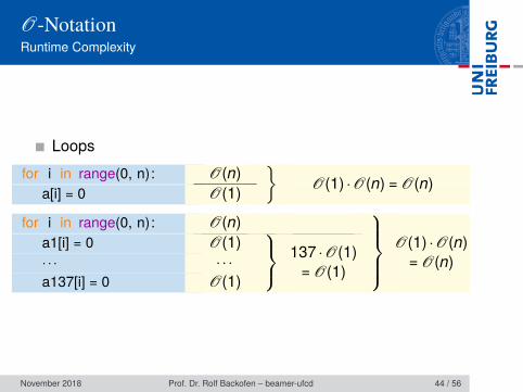
O-NotationRuntime Complexity
Loopsfor i in range(0, n): O(n)
a[i] = 0 O(1)
O(1) ·O(n) = O(n)
for i in range(0, n): O(n)a1[i] = 0 O(1)· · · · · ·a137[i] = 0 O(1)
137 ·O(1)= O(1)
O(1) ·O(n)
= O(n)
November 2018 Prof. Dr. Rolf Backofen – beamer-ufcd 44 / 56
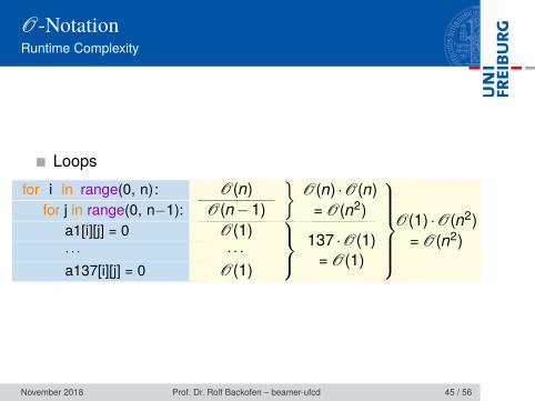
O-NotationRuntime Complexity
Loopsfor i in range(0, n): O(n)
for j in range(0, n−1): O(n−1)
O(n) ·O(n)
= O(n2)a1[i][j] = 0 O(1)· · · · · ·a137[i][j] = 0 O(1)
137 ·O(1)= O(1)
O(1) ·O(n2)
= O(n2)
November 2018 Prof. Dr. Rolf Backofen – beamer-ufcd 45 / 56
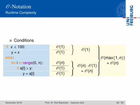
O-NotationRuntime Complexity
Conditionsif x < 100: O(1)
y = x O(1)
O(1)
else:for i in range(0, n): O(n)
if a[i] > y: O(1)y = a[i] O(1)
O(n) ·O(1)= O(n)
O(max1,n)
= O(n)
November 2018 Prof. Dr. Rolf Backofen – beamer-ufcd 46 / 56
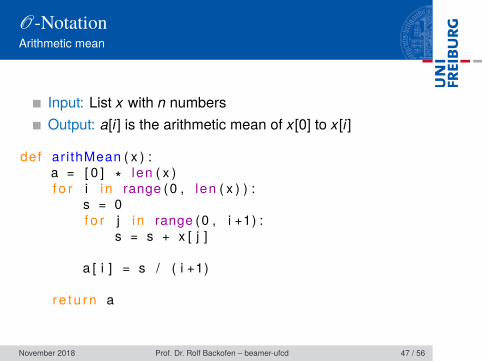
O-NotationArithmetic mean
Input: List x with n numbersOutput: a[i] is the arithmetic mean of x[0] to x[i]
def ar i thMean ( x ) :a = [ 0 ] ∗ len ( x )f o r i i n range (0 , len ( x ) ) :
s = 0f o r j i n range (0 , i +1) :
s = s + x [ j ]
a [ i ] = s / ( i +1)
r e t u rn a
November 2018 Prof. Dr. Rolf Backofen – beamer-ufcd 47 / 56
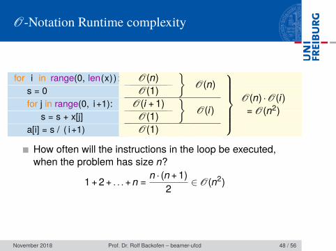
O-Notation Runtime complexity
for i in range(0, len(x)) : O(n)s = 0 O(1)
O(n)
for j in range(0, i+1): O(i +1)s = s + x[j] O(1)
O(i)
a[i] = s / ( i+1) O(1)
O(n) ·O(i)
= O(n2)
How often will the instructions in the loop be executed,when the problem has size n?
1+2+ . . .+ n = n · (n +1)2 ∈ O(n2)
November 2018 Prof. Dr. Rolf Backofen – beamer-ufcd 48 / 56
O-NotationDiscussion
Way of speaking:With the O-Notation we look at the behavior of a functionwhen n→ ∞
We only analyze the runtime when n≥ n0
We talk about asymptotic analysis, when we discuss cost,runtime, etc. as O(. . .), Ω(. . .) or Θ(. . .)
November 2018 Prof. Dr. Rolf Backofen – beamer-ufcd 49 / 56
O-NotationDiscussion
Attention:
If you are using asymptotic analysis, you can not makeany predictions about the runtime of smaller input sizes(n < n0)For small input sizes (mostly n < 10), the runtime ispredictably smalln0 does not necessarily have to be small
November 2018 Prof. Dr. Rolf Backofen – beamer-ufcd 50 / 56
O-NotationDiscussion
Examples:Let A and B be algorithms
A has the runtime f (n) = 80nB has the runtime g(n) = 2n log2n
So f = O(g) but not Θ(g)⇒ A is asymptotic faster than B⇒ There is an n0 for that n≥ n0 : f (n)≤ g(n)
November 2018 Prof. Dr. Rolf Backofen – beamer-ufcd 51 / 56
O-NotationDiscussion
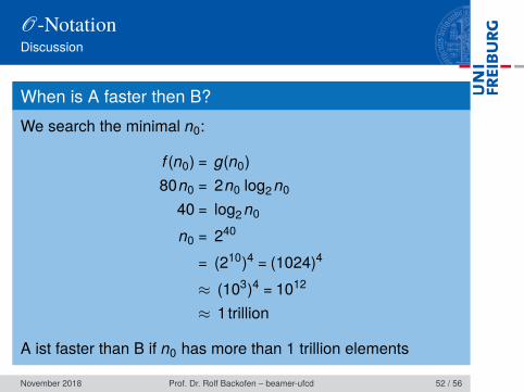
When is A faster then B?We search the minimal n0:
f (n0) = g(n0)80n0 = 2n0 log2n0
40 = log2n0
n0 = 240
= (210)4 = (1024)4
≈ (103)4 = 1012
≈ 1trillion
A ist faster than B if n0 has more than 1 trillion elements
November 2018 Prof. Dr. Rolf Backofen – beamer-ufcd 52 / 56
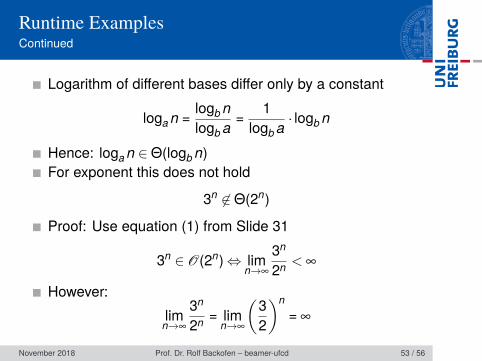
Runtime ExamplesContinued
Logarithm of different bases differ only by a constant
loga n = logb nlogb a = 1
logb a · logb n
Hence: loga n ∈Θ(logb n)For exponent this does not hold
3n 6∈Θ(2n)
Proof: Use equation (1) from Slide 31
3n ∈ O(2n)⇔ limn→∞
3n
2n < ∞
However:limn→∞
3n
2n = limn→∞
(32
)n= ∞
November 2018 Prof. Dr. Rolf Backofen – beamer-ufcd 53 / 56
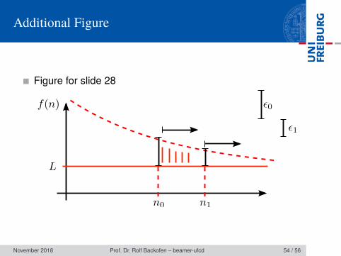
Additional Figure
Figure for slide 28
November 2018 Prof. Dr. Rolf Backofen – beamer-ufcd 54 / 56
Further Literature
General[MS08] Kurt Mehlhorn and Peter Sanders.
Algorithms and data structures, 2008.https://people.mpi-inf.mpg.de/~mehlhorn/ftp/Mehlhorn-Sanders-Toolbox.pdf.
November 2018 Prof. Dr. Rolf Backofen – beamer-ufcd 55 / 56
Further Literature
Big O notation
[Wik] Big O notationhttps://en.wikipedia.org/wiki/Big_O_notation
November 2018 Prof. Dr. Rolf Backofen – beamer-ufcd 56 / 56