![arXiv:1802.01854v2 [math.AP] 10 Apr 2018arXiv:1802.01854v2 [math.AP] 10 Apr 2018 BLOW-UP PROFILE OF ROTATING 2D FOCUSING BOSE GASES MATHIEU LEWIN, PHAN THANH NAM, AND NICOLAS ROUGERIE`](https://static.fdocument.org/doc/165x107/5e900fe147699a4bac5d10c8/arxiv180201854v2-mathap-10-apr-2018-arxiv180201854v2-mathap-10-apr-2018.jpg)
A weak energy identity and the length of necks for a ... · blow-up points). On the other hand,...
51
Advances in Mathematics 225 (2010) 1134–1184 www.elsevier.com/locate/aim A weak energy identity and the length of necks for a sequence of Sacks–Uhlenbeck α -harmonic maps ✩ Yuxiang Li a,∗,1 , Youde Wang b,2 a Department of Mathematical Sciences, Tsinghua University, Beijing 100084, PR China b Academy of Mathematics and Systematic Sciences, Chinese Academy of Sciences, Beijing 100190, PR China Received 13 May 2009; accepted 24 March 2010 Available online 24 April 2010 Communicated by Gang Tian Abstract In this paper we discuss the convergence behavior of a sequence of α-harmonic maps u α with E α (u α )<C from a compact surface (M,g) into a compact Riemannian manifold (N,h) without boundary. Generally, such a sequence converges weakly to a harmonic map in W 1,2 (M,N) and strongly in C ∞ away from a finite set of points in M. If energy concentration phenomena appears, we show a generalized energy identity and discover a direct convergence relation between the blow-up radius and the parameter α which ensures the energy identity and no-neck property. We show that the necks converge to some geodesics. Moreover, in the case there is only one bubble, a length formula for the neck is given. In addition, we also give an example which shows that the necks contain at least a geodesic of infinite length. © 2010 Elsevier Inc. All rights reserved. MSC: 58E20; 35J60 Keywords: Energy identity; Bubble; Neck; α-Harmonic map ✩ This paper was written while the first author was researching at Mathematisches Institut, Albert-Ludwigs-Universität Freiburg, supported by Alexander von Humboldt Foundation. * Corresponding author. E-mail addresses: [email protected] (Y. Li), [email protected] (Y. Wang). 1 Partially supported by the National Science Foundation of China (No. 10801082) and the Specialized Research Fund for the Doctoral Program of Higher Education (No. 200800031078). 2 Partially supported by 973 project of China, Grant No. 2006CB805902, and NSFC, Grant No. 10990013. 0001-8708/$ – see front matter © 2010 Elsevier Inc. All rights reserved. doi:10.1016/j.aim.2010.03.020
Transcript of A weak energy identity and the length of necks for a ... · blow-up points). On the other hand,...
Advances in Mathematics 225 (2010) 1134–1184www.elsevier.com/locate/aim
A weak energy identity and the length of necks fora sequence of Sacks–Uhlenbeck α-harmonic maps ✩
Yuxiang Li a,∗,1, Youde Wang b,2
a Department of Mathematical Sciences, Tsinghua University, Beijing 100084, PR Chinab Academy of Mathematics and Systematic Sciences, Chinese Academy of Sciences, Beijing 100190, PR China
Received 13 May 2009; accepted 24 March 2010
Available online 24 April 2010
Communicated by Gang Tian
Abstract
In this paper we discuss the convergence behavior of a sequence of α-harmonic maps uα withEα(uα) < C from a compact surface (M,g) into a compact Riemannian manifold (N,h) without boundary.Generally, such a sequence converges weakly to a harmonic map in W1,2(M,N) and strongly in C∞ awayfrom a finite set of points in M . If energy concentration phenomena appears, we show a generalized energyidentity and discover a direct convergence relation between the blow-up radius and the parameter α whichensures the energy identity and no-neck property. We show that the necks converge to some geodesics.Moreover, in the case there is only one bubble, a length formula for the neck is given. In addition, we alsogive an example which shows that the necks contain at least a geodesic of infinite length.© 2010 Elsevier Inc. All rights reserved.
MSC: 58E20; 35J60
Keywords: Energy identity; Bubble; Neck; α-Harmonic map
✩ This paper was written while the first author was researching at Mathematisches Institut, Albert-Ludwigs-UniversitätFreiburg, supported by Alexander von Humboldt Foundation.
* Corresponding author.E-mail addresses: [email protected] (Y. Li), [email protected] (Y. Wang).
1 Partially supported by the National Science Foundation of China (No. 10801082) and the Specialized Research Fundfor the Doctoral Program of Higher Education (No. 200800031078).
2 Partially supported by 973 project of China, Grant No. 2006CB805902, and NSFC, Grant No. 10990013.
0001-8708/$ – see front matter © 2010 Elsevier Inc. All rights reserved.doi:10.1016/j.aim.2010.03.020
Y. Li, Y. Wang / Advances in Mathematics 225 (2010) 1134–1184 1135
1. Introduction
Let (M,g) be a smooth compact Riemann surface without boundary, and (N,h) be an n-dimensional smooth compact Riemannian manifold without boundary. By Nash’s isometricembedding theorem, we assume that N is isometrically embedded in some Euclidean spaceN ↪→ R
K for the sequel.We define the Sobolev space of W 1,p-maps from M into N , denoted by W 1,p(M,N), as
W 1,p(M,N) = {u ∈ W 1,p(M,R
K): u(x) ∈ N for a.e. x ∈ M
}.
If u ∈ W 1,2(M,N), we define the energy density e(u) of u by
e(u) = Traceg u∗h = |∇gu|2,where u∗h is the pull-back of the metric tensor h. In a local coordinate system of x ∈ M , theenergy density can be expressed as
e(u)(x) = gij (x)hαβ
(u(x))∂uα
∂xi
∂uβ
∂xj.
The energy E(u) of u is defined by
E(u) =∫M
e(u)dVg,
and the critical points of E(u) are called harmonic maps from M into N . Hence, a harmonic mapu satisfies the corresponding Euler–Lagrange equation in the sense of distribution
τ(u) = �u + A(u)(∇u,∇u) = 0,
where A(·,·) is the second fundamental form of N in RK .
Eells and Sampson first employed the heat flow method to approach the existence problemsof harmonic maps and deformed successfully a map from a closed manifold into a manifold withnon-positive sectional curvature into a homotopic harmonic map. Concretely, they consideredthe heat flow of harmonic maps (or the negative gradient flow of the energy functional E(u)):
∂u
∂t= τ(u).
If one can establish the global existence of the above flow with respect to the time variable t ,or roughly speaking, the flow flows to infinity smoothly, then we are able to find a sequenceuk = u(x, tk) such that uk converges to a harmonic map as tk → +∞ (see [9]). Generally, sucha flow does not exist globally (see [6] and [2]).
From the view point of calculus of variations, it is also not easy to find a harmonic map,since E does not satisfy the well-known Palais–Smale condition when the dimensions of do-main manifold dim(M) � 2. In particular, when dim(M) = 2, it is well known that the energyfunctional E is of conformal invariance and the corresponding variational problem possesses anon-compact invariance group and represents limiting cases where the Palais–Smale condition
1136 Y. Li, Y. Wang / Advances in Mathematics 225 (2010) 1134–1184
just fails. Therefore, harmonic maps from a surface are of special importance and interest. Infact, mathematicians have paid more attention to this case. To prove the existence of harmonicmaps from a closed surface Sacks and Uhlenbeck in their pioneering paper [17] introduced aperturbed energy functional which satisfies the Palais–Smale condition, hence obtained so calledα-harmonic maps, as critical points of perturbed functional, to approximate harmonic maps.More precisely, for every u ∈ W 1,2α(M,N) Sacks and Uhlenbeck defined the so called α-energyfunctional Eα as
Eα(u) =∫M
(1 + |∇u|2)α dVg,
which can be regarded as a perturbation of energy functional E, and considered α-harmonicmaps, i.e. the critical points of Eα in W 1,2α(M,N), which satisfy the following equation:
�guα + (α − 1)∇g|∇guα|2∇guα
1 + |∇guα|2 + A(uα)(duα, duα) = 0. (1.1)
We call such an α-harmonic map as Sacks–Uhlenbeck α-harmonic map. If there is a subsequenceuαk
which converges smoothly as αk → 1, then uαkwill converge to a harmonic map. Such
smooth convergence fails generally, thus, Sacks and Uhlenbeck developed a powerful methodand some techniques to investigate the blow-up phenomena for such a variational problem.
Later, Struwe [18] used the heat flow method of Eells and Sampson to approach the existenceproblems for harmonic maps from a closed surface and he obtained almost the same results asin [17]. Chang showed the same results as in [18] for the case where the domain manifold is acompact surface with smooth boundary (see [1]).
No matter which method, Sacks–Uhlenbeck perturbation or heat flow approach, is adoptedto produce a sequence of two-dimensional approximate harmonic maps, generally we cannotexclude the bubbling phenomena when we consider the convergence of such a sequence. Thatis to say, it is possible that the limiting map (a smooth harmonic map u0) is just a trivial map,although such a sequence converges smoothly away from finitely many points (which are calledblow-up points). On the other hand, around every blow-up point p, the energy concentrates andthere are some non-trivial harmonic maps wi from S2 to N , i.e. some bubbles for the sequenceof approximate harmonic maps.
For a sequence of approximate harmonic maps from a compact Riemann surface M into N
with bounded energy, naturally one pays attention to the following two problems: One is whetherthe energy identity holds true or not, i.e.
limk→+∞
∫M
|∇uk|2 dVg =∫M
|∇u0|2 dVg +m∑
i=1
E(wi)?
where m is the number of all bubbles. The other is what we can say about necks joining bubblesif they exist?
When uk = u(x, tk) is a subsequence of a heat flow for two-dimensional harmonic maps, theabove two problems were deeply studied. The energy identities have been proved by Qing [15](for the case N = Sn), Ding and Tian [7] for the general case. Lin and Wang provided anotherproof of the energy identity in [13]. Furthermore, Qing and Tian [16] proved that there is no
Y. Li, Y. Wang / Advances in Mathematics 225 (2010) 1134–1184 1137
neck if blow-up phenomena happens at infinite time and Ding [5] proved a more general result.It is worthy to point out that Topping [19] provided a surprising example of heat flow u(x, t) forwhich the blow-up phenomena appears at a finite time T and the weak limit limt→T u(x, t) isnot continuous. Also, one has known that for some special sequences of α-harmonic maps theenergy identity is true. But it was obtained by some methods which are completely different fromthe one of [7]. Now we would like to mention the following cases.
If {uα} is a sequence of minimizing α-harmonic maps (every uα is the minimizer of Eα), eachuα of which belongs to the same homotopy class, Chen and Tian [3] proved that the necks consistof some geodesics of finite length, and moreover this implies no loss of energy in necks for thesequence, i.e. the energy identity holds true.
Jost considered the energy identity for a minimax sequence of α-harmonic maps. Supposethat M is a compact Riemann surface and A is a parameter manifold. Let h0 :M × A → N be acontinuous map, and H be the set of such continuous maps h :M ×A → N that h are homotopicto h0 and satisfy h(t) ∈ W 1,2α(M,N) for any fixed t ∈ A. Set
βα(H) = infh∈H
supt∈A
Eα
(h(·, t)).
We can deduce from Jost’s result [10] that there is at least a sequence {uαk}, which attained
βαk(H), satisfies the energy identity as αk → 1. Recently, T. Lamm gave a simple proof of this
energy identity [11] (also see [4] and [14]).The energy identity for an α-harmonic map sequence with bounded energy is still open up
to now. It seems that the methods used to show the identity for heat flow, or a sequence ofapproximate maps with tension fields τ bounded in L2, are not powerful enough to prove theenergy identity for such an α-harmonic map sequence. We think that the key difficulty lies on theidentity (2.5) in this paper. Indeed, for a sequence of maps with tension fields τ bounded in L2,then from (2.5) we can see easily
∫∂Br
∣∣∣∣∂uk
∂r
∣∣∣∣2
ds0 − 1
2
∫∂Br
|∇0uk|2 ds0 = O
( ∫Br
∣∣τ(uk)∣∣|∇uk|dVg
)+ O(1),
then the right-hand side of the above identity is bounded, therefore we can derive the energyidentity for heat flow or a sequence of maps with tension fields τ bounded in L2. However, for asequence of α-harmonic maps a very “bad” term
α − 1
r
∫Br
(1 + |∇uα|2)α−1|∇uα|2 dVg
appears in (2.5). We will see that it is not so easy to control such a term.In this paper, we attempt to establish a generalized energy identity and study the asymptotic
behaviors of neck domains. When we encounter the situation at a blow-up point there are severalbubbles of a sequence of α-harmonic maps, we will be concerned with more general α-energyfunctionals which are of the following forms:
Eα,εα (u) =∫ (
εα + |∇guα|2)α dVgα ,
M
1138 Y. Li, Y. Wang / Advances in Mathematics 225 (2010) 1134–1184
where α > 1 and 0 < εα < 1. In the beginning of Section 2, furthermore it will be explainedwhy one needs to consider such a kind of functionals. On the other hand, also it is of interestto consider whether a sequence of critical points corresponding such a family of functionalsconverges or not.
In consideration of the above motivations and reasons, more precisely we will focus on thefollowing problems: “Given a sequence of maps uα from (Bσ , gα) to (N,h), each of which is acritical point of the corresponding Eα,εα (u), with Eα,εα (uα) � Θ and
0 < β0 < limα→1
εαα−1 � 1.
Here Θ and β0 are positive constants, Bσ is a ball in R2 centered at the origin, and gα =
eϕα ((dx1)2 + (dx2)2) with ϕα(0) = 0 and ϕα → ϕ ∈ C∞(Bσ ) smoothly. Moreover, without lossof generality we assume that uα → u0 in Ck
loc(Bσ \ {0}). For such a sequence {uα}, does the en-ergy identity hold true? If the necks joining bubbles exist, do the necks consist of some geodesics?And if so, can we give the length formula of such geodesics?”
We will adopt some methods and techniques in [7] and [5] to discuss the above problems. Inorder to make detailed analysis on the energy on neck domains, we will employ some suitablevariational formulas to establish some useful integral identities, and make use of ε-regularitytheory and blow-up analysis to derive some a priori estimates by which the “bad” term mentionedin the above can be controlled effectively. We only show a weak energy identity for such asequence. On the other hand, we also study the convergence behaviors of the neck domains.Precisely, we provide a new method to show that the necks converge to geodesics and obtaina formula on the length of the geodesics. In particular, we discover the relation between theblow-up radius and the parameter α which ensures the energy identity and no-neck property.
In order to state our main results, here we introduce some basic facts about harmonic mapsand some related notions which are needed for the sequel. For a more detailed discussion of thefacts reviewed here, we refer the reader to various articles cited below.
It is well known that there always exists an isothermal coordinate system in a small neighbor-hood of every p ∈ M since dim(M) = 2, i.e. there is a real function ϕ with ϕ(p) = 0 such thatthe metric can be locally expressed as
ds2M = eϕ
((dx1)2 + (dx2)2).
As the energy functional E is invariant under conformal transformations, so, essentially we onlyneed to consider the blow-up phenomena in a small ball Br in Euclidean plane, centered at theorigin, with a metric given by g = eϕ((dx1)2 + (dx2)2) where ϕ is a smooth real function on Br
satisfying ϕ(0) = 0.Now, we assume that {uα} (α → 1) is a sequence of α-harmonic maps from (M,g) to (N,h)
with bounded α-energy, i.e.
Eα,εα (uα) < Θ.
Then, by the theory of Sacks and Uhlenbeck, there exists a sequence of αk-harmonic maps uαk
which converges to a harmonic map u0 :M → N smoothly away from finitely many points {xi}as αk → 1. Furthermore, we suppose that there are n0 bubbles at a singular point x1. Then, forevery j ∈ {1, . . . , n0} there are a sequence of points {xj
α ∈ M: k ∈ Z} with xjα → x1 as αk → 1,
k k
Y. Li, Y. Wang / Advances in Mathematics 225 (2010) 1134–1184 1139
and a sequence of positive real numbers {λjαk
: k ∈ Z} with λjαk
→ 0 as αk → 1, such that thesequence of maps given by
vjαk
= uαk
(xjαk
+ λjαk
x)
converges in Ckloc(R
2 \ {pj
1 ,pj
2 , . . . , pjsj }) to a non-trivial harmonic map, denoted by
vj :S2 → N, j = 1,2, . . . , n0.
Moreover, one of the following always holds true:
(H1) For any fixed R > 0, BRλiα(xi
α) ∩ BRλ
jα(x
jα) = ∅ whenever (α − 1) are sufficiently small.
(H2) λiα
λjα
+ λjα
λiα
→ +∞ as α → 1.
Remark 1.1. One is easy to check that if (λiα, xi
α) and (λjα, x
jα) do not satisfy (H1) and (H2), then
one is able to find subsequences of λiα , xi
α and λjα , x
jα such that
λiα
λjα
→ λ ∈ (0,∞) andxiα − x
jα
λjα
→ a ∈ R2.
Since
uα
(xiα + λi
αx)= uα
(xjα + λj
α
(xiα − x
jα
λjα
+ λiα
λjα
x
)),
we have vi(x) = vj (a + λx), and then vi and vj are in fact the same bubbles.
In order to reveal the relation between the blow-up radius and the parameter α which ensuresthe energy identity and no-neck property, we need to introduce the following quantities:
μj ≡ lim infα→1
(λj
α
)2−2α (1.2)
and
νj ≡ lim infα→1
(λj
α
)−√α−1
. (1.3)
Obviously, νj ∈ [1,∞]. It is also easy to see that μj ∈ [1,μmax] for some positive numberμmax � 1 (see Remark 1.2). We will see that the quantities μj and νj characterize completelythe energy identity and the length of necks joining bubbles respectively.
Now, we are in the position to state our main results. The first task of this paper is to establishthe following weak energy identity:
Theorem 1.1. Let Bσ = Bσ (0) be a ball in R2, gα = eϕα(x)((dx1)2 + (dx2)2) and g0 =
eϕ(x)((dx1)2 + (dx2)2) be a family of metrics on Bσ , where ϕα ∈ C∞(Bσ ), ϕα(0) = 0, and
1140 Y. Li, Y. Wang / Advances in Mathematics 225 (2010) 1134–1184
ϕα converges smoothly to ϕ ∈ C∞(Bσ ). Assume uα : (Bσ , gα) → N (α → 1) is a sequence ofmaps, each uα of which is a critical point of the corresponding functional Eα,εα (u,Bσ ), withEα,εα (uα,Bσ ) < Θ for any 0 < α � 1 and
0 < β0 < limα→1
εαα−1 � 1;
moreover, uα → u0 in C∞loc(Bσ \ {0},N) and there are n0 bubbles vj :S2 → N at point {0}. Here
Θ and β0 are positive constants. Then the following energy identity holds true
limδ→0
limα→1
∫Bδ(0)
(εα + |∇gαuα|2)α dVgα =
n0∑j=1
μ2jE(vj),
where μj is defined by (1.2).
Remark 1.2. We claim that in Theorem 1.1 μj ∈ [1,μmax] for some bounded positive num-ber μmax. Indeed, fixing an R > 0, we have
∫B
Rλjαk
(xjαk
)\(⋃sji=1 B
δλjαk
(xjαk
+λjαk
pji ))
|∇guαk|2αk dVg
= (λjαk
)2−2α∫
BR(xjαk
)\(⋃sji=1 Bδ(x
jαk
+pji ))
∣∣∇gvjαk
∣∣2αk dVg(x
jαk
+λjαk
x). (1.4)
Since λjαk
< 1, xjαk
→ 0 and
limαk→1
∫BR(x
jαk
)\(⋃sji=1 Bδ(x
jαk
+pji ))
∣∣∇gvjαk
∣∣2αk dVg(x
jαk
+λjαk
x)→
∫BR\(⋃sj
i=1 Bδ(pji ))
∣∣∇0vj∣∣2 dx,
then we have for large R and small δ
μj � limαk→1
∫B
Rλjαk
(xjαk
)\(⋃sji=1 B
δλjαk
(xjαk
+λjαk
pji ))
|∇gujαk
|2αk dVg∫BR\(⋃sj
i=1 Bδ(pji ))
|∇0vj |2 dx.
Therefore, there holds
μj � limδ→0
limR→∞ lim
αk→1
∫B
Rλjαk
(xjαk
)\(⋃sji=1 B
δλjαk
(xjαk
+λjαk
pji ))
|∇gujαk
|2αk dVg∫BR\(⋃sj
i=1 Bδ(pji ))
|∇0vj |2 dx
� 1(Θ −(
lim inf εαk
)|Bσ | − E(u0,Bσ )
)≡ μmax, (1.5)
θ αk→1
Y. Li, Y. Wang / Advances in Mathematics 225 (2010) 1134–1184 1141
where BR = BR(0) is a ball in R2, |Bσ | denotes the area of Bσ and
θ = inf{E(u): all non-trivial harmonic maps u from S2 into N
}.
This theorem tells us that the energy identity holds true if and only if μj = 1. It provides anew route to approach the problem whether the energy on necks vanishes or not. Obviously, inthe above theorem u0 is a harmonic map from (Bσ , g0) into N . As a direct corollary, we obtain
Theorem 1.2. Let M be a smooth closed Riemann surface and N be a smooth compact Rie-mannian manifold without boundary. Assume that uαk
∈ C∞(M,N) (αk → 1) is a sequenceof αk-harmonic maps with uniformly bounded α-energy, i.e. Eαk
(uαk) � Θ , and x1 be the only
blow-up point of the sequence {uαk} in Bσ (x1) ⊂ M . Then, passing to a subsequence, there exist
u0 :M → N which is a smooth harmonic map and finitely many bubbles vj :S2 → N such thatuαk
→ u0 weakly in W 1,2(M,N), and in C∞loc(Bσ (x1)\{x1},N); and the following identity holds
limk→+∞Eαk
(uαk
,Bσ (x1))= E
(u0,Bσ (x1)
)+ ∣∣Bσ (x1)∣∣+ n0∑
j=1
μ2jE(vj), (1.6)
where μj is defined by (1.2) and n0 is the number of bubbles at blow-up point x1.
It is our another purpose to study the properties of the necks joining bubbles. Our main resultsare stated as follows:
Theorem 1.3. Let Bσ = Bσ (0) be a ball in R2, gα = eϕα(x)((dx1)2 + (dx2)2) and g0 =
eϕ(x)((dx1)2 + (dx2)2) be a family of metrics on Bσ , where ϕα ∈ C∞(Bσ ), ϕα(0) = 0, andϕα converges smoothly to ϕ ∈ C∞(Bσ ). Assume uα : (Bσ , gα) → N is a sequence of α-harmonicmaps as stated in Theorem 1.1, and there is only one bubble v1 :S2 → N in Bσ for such asequence and the blow-up point is {0}. Then we have
1) when ν1 = 1, the set u0(Bσ ) ∪ v1(S2) is a connected subset of N ;2) when ν1 ∈ (1,∞), the set u0(Bσ ) and v1(S2) are connected by a geodesic with length
L =√
E(v1)
πlogν1;
3) when ν1 = +∞, the neck contains at least an infinite length geodesic.
Here ν1 is defined by (1.3), i.e. ν1 = lim infα→1(λ1α)−
√α−1.
As a direct corollary, we have
Theorem 1.4. Let M be a smooth closed Riemann surface and N be a smooth closed Rie-mannian manifold and uαk
∈ C∞(M,N) be a sequence of αk-harmonic maps with uniformlybounded energy, i.e. Eαk
(uαk) � Θ , and uαk
converges to a smooth harmonic map u0 :M → N
in C∞loc(Bσ (x1) \ {x1},N) as αk → 1. Assume there is only one bubble in Bσ (x1) ⊂ M for {uαk
}and v1 :S2 → N is the bubbling map. Let ν1 = lim infα→1(λ
1 )−√
α−1. Then we have
α
1142 Y. Li, Y. Wang / Advances in Mathematics 225 (2010) 1134–1184
1) when ν1 = 1, the set u0(Bσ (x1)) ∪ v1(S2) is a connected subset of N ;2) when ν1 ∈ (1,∞), the set u0(Bσ (x1)) and v1(S2) are connected by a geodesic with length
L =√
E(v1)
πlogν1;
3) when ν1 = +∞, the neck contains at least an infinite length geodesic.
We should mention that after we completed the paper we found that Moore had proved thatthe same length formula holds true if a neck is of finite length L and g � 1 (the genus of M).Note that E(u) is defined by 1
2
∫M
|∇u|2 dVg in [14]. However, in this paper the arguments toprove Theorem 1.3 is completely different from Moore’s proof. The key estimations, which givethe details of the necks, are established in Proposition 4.3 in Section 4.
We fail to find a sufficient condition such that νi < +∞, but we will show that there areindeed many cases that the necks contain at least a geodesic of infinite length:
Corollary 1.5. Let {uαk} (αk → 1) be a sequence of maps from M into N each uαk
of which isa minimizer of Eαk
in the homotopy class containing uαk. We assume that, for any αi = αj , uαi
and uαjdo not belong to a homotopy class. If
supαk
Eαk(uαk
) < +∞,
then {uαk} blows up at some points, and the necks contain at least a geodesic of infinite length.
Remark 1.3. In Section 5, by constructing a compact manifold N we give an example of se-quence of minimizing α-harmonic maps, which satisfies the conditions in the above corollary.This indicates that there exists a neck joining bubbles which is a geodesic of infinite length.
As a consequence of Theorem 1.1, we have the following proposition which implies the resultdue to Chen–Tian that, if the necks consist of some geodesics of finite length, then the energyidentity is true:
Proposition 1.6. The energy identity holds true for a subsequence of uα if and only if
lim infα→1
‖∇uα‖α−1C0(M)
= 1. (1.7)
The limit set of such subsequence has no neck if and only if
lim infα→1
‖∇uα‖√
α−1C0(M)
= 1.
The bubbles in limit set of such subsequence are joined by some geodesics of finite length, if andonly if
lim infα→1
‖∇uα‖√
α−1C0(M)
< +∞.
Y. Li, Y. Wang / Advances in Mathematics 225 (2010) 1134–1184 1143
Proof. We only prove the first claim. First, we prove that (1.7) implies μj = 1. We assume
vjα(x) = uα(x
jα + λ
jαx) converges to vj in C1
loc(Rn \ {p1,p2, . . . , ps}). Then we have
(λj
α
)1−α = |∇uα(xjα + λ
jαx)|α−1
|∇vjα(x)|α−1
for any x with |∇vj (x)| = 0. Hence we get μj � 1 and then μj = 1.Conversely, if μj = 1 for all j , we need to verify (1.7). Let xα ∈ M be the point such that
|∇uα(xα)| = maxM |∇uα|, and
λα = 1
|∇uα(xα)| .
We set vα(x) = uα(xα + λαx). One is easy to check that vα will converge to a non-trivial har-monic map v0 locally. By (H1) and (H2) we must have j , such that
BRλ
jα
(xjα
)∩ BRλα (xα) = ∅, and1
Cλj
α < λα < Cλjα
for some C > 0. Hence we get |λα|α−1 → 1. �The paper is organized as follows: In Section 2 we recall the well-known ε-regularity theorem
due to Sacks and Uhlenbeck, and establish some gradient estimates and integral estimates. Weshow Theorem 1.1 in Section 3. We analyze the asymptotic behaviors of the neck domains andgive the length formula of the neck in Section 4 for the case only one bubble appears. In Section 5,an example of sequence of maps is given to show the necks contain at least a geodesic of infinitelength. In Section 6, we indicate how to construct the bubble tree of a sequence of α-harmonicmaps.
2. Preliminary
In this section we intend to establish some integral formulas on α-harmonic maps from acompact closed surfaces by the variations of domain. Of course, we need to choose some suitablevariational vector fields on M which generate the transformations of M . We will see that theseintegral relations will play an important role on the proofs of main theorems.
Now, we give the reasons and motivations to study the functionals Eα,εα stated in Section 1.Recall that the functional Eα is not of conformal invariance. For example, on an isothermalcoordinate system around a point p ∈ M , if the metric is given by g = eϕ((dx1)2 + (dx2)2) withϕ(p) = 0 and uα(x) = uα(λx), then we have
∫Bδ(p)
(1 + |∇guα|2)α dVg =
∫B δ (p)
λ2−2α(λ2 + |∇g′ uα|2)α dVg′,
λ
1144 Y. Li, Y. Wang / Advances in Mathematics 225 (2010) 1134–1184
where g′ = eϕ(p+λx)((dx1)2 + (dx2)2). On the other hand, we should also note that, for a se-quence of α-harmonic maps uα , it is possible that there exist several bubbles near a blow-uppoint. For example, if there are sequences {λ1
α} and {λ2α} such that
λ2α/λ1
α → 0, λ1α → 0,
as α → 1, and
v1α(x) = uα
(λ1
αx)→ v1 in Ck
loc
(R
2), v2α(x) = uα
(λ2
αx)→ v2 in Ck
loc
(R
2 \ {0}),where v1, v2 are non-trivial harmonic maps from S2 to N . For this case, we have
v2α(x) = v1
α
((λ2
α/λ1α
)x),
i.e. v2(x) is in fact a bubble for the sequence v1α . Therefore, we have to consider the Euler–
Lagrange equation satisfied by v1α . It is easy to check that v1
α is locally a critical point of thefunctional
F(v) =∫Bδ
((λ1
α
)2 + |∇v|2)α dVgα ,
where gα = eϕ(p+λ1αx)((dx1)2 + (dx2)2). For the above reasons, we need to consider more gen-
eral α-energy functionals which are of the following forms:
Eα,εα (u) =∫B
(εα + |∇guα|2)α dVgα ,
where B = {x: |x| < 1} is a unit ball in R2 and εα ∈ (0,1]. If uα is a critical point of the above
some functional Eα,εα (u), then, uα satisfies the following elliptic system which is also calledα-harmonic map equation:
�gαuα + (α − 1)∇gα |∇gαuα|2∇gαuα
εα + |∇gαuα|2 + A(uα)(duα, duα) = 0. (2.1)
Here we always assume that the sequence εα (εα � 1) satisfies
limα→1
εαα−1 > β0 > 0. (2.2)
From (1.5) we can see that this assumption is reasonable.Next, we recall the well-known ε-regularity theorem due to Sacks and Uhlenbeck [17]:
Theorem 2.1. Let uα : (B,gα) → N satisfies Eq. (2.1). Then, there exists ε > 0 and α0 > 1 suchthat if E(uα,B) < ε and 1 � α � α0, then for all smaller r < 1, we have
‖∇gαuα‖W 1,p(Br )� C(p, r)E(uα,B),
here Br ⊂ B is a ball with radius r , 1 < p < ∞.
Y. Li, Y. Wang / Advances in Mathematics 225 (2010) 1134–1184 1145
Remark 2.1. It is worthy to point out that the constant C(p, r) in Theorem 2.1 does not dependon α, εα and gα if gα = eϕα ((dx1)2 +(dx2)2), where ϕα(0) = 0 and ϕα → ϕ ∈ C∞(B) smoothly.
We also have the following a priori estimates:
Lemma 2.2. Let (B,gα) be a unit disk in R2 with metric gα = eϕα ((dx1)2 + (dx2)2), where
ϕα(0) = 0 and ϕα → ϕ ∈ C∞(B) smoothly. If uα : (B,gα) → N is a critical point of Eα,εα (u,B)
given by
Eα,εα (u,B) =∫B
(εα + |∇gαuα|2)α dVgα ,
with limα→1 εαα−1 > β0 > 0 and Eα,εα (uα) � Θ , then we have
β0 < lim infα→1
∥∥(εα + |∇gαuα|2)α−1∥∥C0(B)
� lim supα→1
∥∥(εα + |∇gαuα|2)α−1∥∥C0(B)
< β1,
where β1 is independent of α.
Proof. Obviously, we only need to prove ‖∇gαuα‖α−1C0(B)
< C. We assume that there is a sequence
of {uαk} such that ‖∇gαk
uαk‖αk−1C0(B)
→ +∞ as αk → 1. Suppose that max{|∇gαkuαk
|} is attainedat xαk
, i.e.
∣∣∇gαkuαk
(xαk)∣∣= max
B
{|∇gαkuαk
|}.Let λk = 1
|∇gαkuαk
(xαk)| and vk(x) = uαk
(xαk+ λkx). Obviously, we have Eαk
(vk) � C < ∞.
Then there exists a subsequence of {vkj} which converges to a new non-trivial harmonic map
from S2 to N . Hence, from (1.5) we can infer λ1−αkj
kj< C, which contradicts with the choice
of αk . �Next we need to establish some general variational formulas for the functional Eα,εα (u,B).
By virtue of these variational identities we can derive some important estimates on the energy onthe necks of the critical points of Eα,εα . The integral identities in the following two lemmas, i.e.(2.6) and (2.8), will be used repeatedly in our arguments.
Lemma 2.3. Let (B,gα) be a unit disk in R2 with metric gα = eϕα ((dx1)2 + (dx2)2), where
ϕα(0) = 0 and ϕα → ϕ ∈ C∞(B) smoothly. If uα is a critical point of Eα,εα (u,B) where 1 �limα→1 εα
α−1 > β0 > 0, then, there holds true for any t < 1
(1 − 1
2α
) ∫∂Bt
(εα + |∇gαuα|2)α−1
∣∣∣∣∂uα
∂r
∣∣∣∣2
ds0 − 1
2α
∫∂Bt
(εα + |∇gαuα|2)α−1|uα,θ |2 ds0
= (α − 1)
αt
∫ (εα + |∇gαuα|2)α−1|∇0uα|2 dx + O(t),
Bt
1146 Y. Li, Y. Wang / Advances in Mathematics 225 (2010) 1134–1184
where ds0 is the volume element and ∇0 is the gradient operator with respect to Euclideanmetric.
Proof. Take a 1-parameter family of transformations {φs} which is generated by the vectorfield X. If we assume X is supported in B , then we have
Eα,εα (u ◦ φs) =∫B
(εα + ∣∣∇gα (u ◦ φs)
∣∣2)α dVgα =∫B
(εα +
∑β
∣∣d(u ◦ φs)(eβ(x)
)∣∣2)α
dVgα
=∫B
(εα +
∑β
∣∣du(φs∗(eβ(x)
))∣∣2)α
dVgα
=∫B
(εα +
∑β
∣∣du(φs∗(eβ
(φ−1
s (x))))∣∣2)α
Jac(φ−1
s
)dVgα ,
where {eα} is a local orthonormal basis of TB. Noting
d
dsJac(φ−1
s
)dVgα
∣∣s=0 = −div(X)dVgα ,
by differentiating the above identity we obtain the formula
dEα,εα (u)(u∗(X)
)= −∫B
(εα + |∇gαu|2)α div(X)dVgα
+ 2α∑β
∫B
(εα + |∇gαu|2)α−1⟨
du(∇eβ X), du(eβ)⟩dVgα .
Now, we assume uα to be the critical point of Eα,εα . For any vector field X on B , we have
2α∑β
∫B
(εα + |∇gαuα|2)α−1⟨
duα(∇eβ X), duα(eβ)⟩dVgα
=∫B
(εα + |∇gαuα|2)α divX dVgα . (2.3)
Next, for 0 < t ′ < t � ρ < 1, we choose a vector field X with compact support in Bρ byX = η(r)r ∂
∂r= η(|x|)xi ∂
∂xi , where η is defined by
η(r) =⎧⎨⎩
1 if r � t ′,t−rt−t ′ if t ′ � r � t,
0 if r � t,
where r =√(x1)2 + (x2)2. By a direct computation we obtain
Y. Li, Y. Wang / Advances in Mathematics 225 (2010) 1134–1184 1147
∇ ∂
∂x1X = η
∂
∂x1+ η′ (x1)2
r
∂
∂x1+ η′ x1x2
r
∂
∂x2+ ηx1Γ 1
11∂
∂x1
+ ηx1Γ 211
∂
∂x2+ ηx2Γ 1
12∂
∂x1+ ηx2Γ 2
12∂
∂x2.
Here Γ kij are the coefficients of Levi-Civita connection with respect to gα . Then,
∑β
⟨duα(∇eβ X), duα(eβ)
⟩dVgα
=⟨duα
(∇ ∂
∂x1X), duα
(∂
∂x1
)⟩dx +
⟨duα
(∇ ∂
∂x2X), duα
(∂
∂x2
)⟩dx
=(
η|∇0uα|2 + η′r∣∣∣∣∂uα
∂r
∣∣∣∣2
+ O(|x|)|∇0uα|2
)dx, (2.4)
where ∇0 is the gradient operator with respect to standard Euclidean metric.It is also easy to check
div(X) = 2η + rη′ + rη∂ϕ
∂r.
Hence, by substituting the above identity and (2.4) into (2.3) we derive
0 = (2α − 2)
∫Bt
η(εα + |∇gαuα|2)α−1|∇0uα|2 dx +
∫Bt
O(|x|)(εα + |∇gαuα|2)α−1|∇0uα|2 dx
− 2εα
∫Bt
η(εα + |∇gαuα|2)α−1
dVgα + εα
t − t ′
∫Bt\Bt ′
r(εα + |∇gαu|2)α−1
dVgα
+ 1
t − t ′
∫Bt\Bt ′
(εα + |∇gαuα|2)α−1
[|∇0uα|2r − 2αr
∣∣∣∣∂uα
∂r
∣∣∣∣2]
dx
−∫Bt
εα
(εα + |∇gαuα|2)α−1
rη∂ϕ
∂rdVgα .
Letting t ′ → t in the above identity and using Lemma 2.2, we obtain the following
∫∂Bt
(εα + |∇gαuα|2)α−1
∣∣∣∣∂uα
∂r
∣∣∣∣2
ds0 − 1
2α
∫∂Bt
(εα + |∇gαuα|2)α−1|∇0uα|2 ds0
= (α − 1)
αt
∫Bt
(εα + |∇gαuα|2)α−1|∇0uα|2 dx + O(t), (2.5)
where ds0 is the volume element of ∂Bt with respect to Euclidean metric.
1148 Y. Li, Y. Wang / Advances in Mathematics 225 (2010) 1134–1184
Note the metric gα can be written as gα = eϕα (dr2 + r2 dθ2) in the polar coordinate system.Set
uα,θ = 1
r
∂uα
∂θ.
Obviously
|∇0uα|2 =∣∣∣∣∂uα
∂r
∣∣∣∣2
+ |uα,θ |2.
Hence, we get from the above identity and (2.5)
(1 − 1
2α
) ∫∂Bt
(εα + |∇gαuα|2)α−1
∣∣∣∣∂uα
∂r
∣∣∣∣2
ds0 − 1
2α
∫∂Bt
(εα + |∇gαuα|2)α−1|uα,θ |2 ds0
= (α − 1)
αt
∫Bt
(εα + |∇gαuα|2)α−1|∇0uα|2 dx + O(t). (2.6)
Thus we finish the proof of the lemma. �We also need to infer a special kind of variational formulas which is derived from the varia-
tions with respect to radial direction, i.e. the following Pohozaev identity.
Lemma 2.4. Let (B,gα) be a unit disk in R2 with metric gα = eϕα ((dx1)2 + (dx2)2), where
ϕα(0) = 0. If uα is a critical point of Eα,εα (u,B), then there holds true for any t < 1
∫∂Bt
(∣∣∣∣∂uα
∂r
∣∣∣∣2
− |uα,θ |2)
ds0 = −2(α − 1)
t
∫Bt
∇0|∇gαuα|2∇0uα
εα + |∇gαuα|2 r∂uα
∂rdx,
where ∂∂r
denotes the radial derivative.
Proof. Denote �0 = ∂2
∂(x1)2 + ∂2
∂(x2)2 . Since uα is a critical point of Eα,εα (u,B), for each α � 1,uα satisfies the Euler–Lagrange equation (2.1), i.e.
�0uα + (α − 1)∇0|∇gαuα|2∇0uα
εα + |∇gαuα|2 + A(uα)(duα, duα) = 0.
As in [13], we multiply the both sides of the above equation with r ∂uα
∂rto obtain
∫r∂uα
∂r�0uα dx = −(α − 1)
∫ ∇0|∇gαuα|2∇0u
εα + |∇gαuα|2 r∂uα
∂rdx.
Bt Bt
Y. Li, Y. Wang / Advances in Mathematics 225 (2010) 1134–1184 1149
It is easy to see
∫Bt
r∂uα
∂r�0uα dx =
∫∂Bt
r
∣∣∣∣∂uα
∂r
∣∣∣∣2
ds0 −∫Bt
∇0
(r∂uα
∂r
)∇0uα dx.
Since
∫Bt
∇0
(r∂uα
∂r
)∇0uα dx =
∫Bt
∇0
(xk ∂uα
∂xk
)∇0uα dx
=∫Bt
|∇0uα|2 dx +t∫
0
2π∫0
r
2
∂(|∇0uα|2)∂r
r dθ dr
=∫Bt
|∇0uα|2 dx + 1
2
∫∂Bt
|∇0uα|2t ds0 −∫Bt
|∇0uα|2 dx
= 1
2
∫∂Bt
|∇0uα|2t ds0,
then, we have
∫∂Bt
(∣∣∣∣∂uα
∂r
∣∣∣∣2
− 1
2|∇0uα|2
)ds0 = −α − 1
t
∫Bt
∇0|∇guα|2∇0uα
εα + |∇guα|2 r∂uα
∂rdx. (2.7)
Immediately, it follows
∫∂Bt
(∣∣∣∣∂uα
∂r
∣∣∣∣2
− |uα,θ |2)
ds0 = −2(α − 1)
t
∫Bt
∇0|∇guα|2∇0uα
εα + |∇guα|2 r∂uα
∂rdx. (2.8)
Thus, we complete the proof. �3. The proof of Theorem 1.1
In this section, we make effort to establish a weak energy identity for a sequence of α-har-monic maps. We will follow the idea of Ding and Tian in [7] and apply (2.6) and (2.8) to showTheorem 1.1. We lay emphasis on the arguments on the case only one bubble occurs for thesequence of α-harmonic maps.
3.1. The weak energy identity for the case of only one bubble
In this subsection we prove Theorem 1.1 in the case of n0 = 1, where n0 is the number of thebubbles. The proof for the cases of several bubbles will be given in the next subsection.
1150 Y. Li, Y. Wang / Advances in Mathematics 225 (2010) 1134–1184
By the assumptions in Theorem 1.1, we know that uα : (Bσ , gα) → N is a sequence of α-har-monic maps with
Eα,εα (uα,Bσ ) < Θ and 0 < β0 < limα→1
εαα−1 � 1.
Each uα satisfies the corresponding equation (2.1).Moreover, there exists a harmonic map u0 from (Bσ , g0) to N such that uα → u0 in Ck
loc(Bσ \{0}) and {0} is the only blow-up point of {uα} in Bσ . Therefore, by the discussions in Lemmas 2.3and 2.4 we know that for any α > 1, uα satisfy (2.6) and (2.8).
We need to define some important quantities related to the energy on necks. In the sequel, wealways pick xα such that
∣∣∇gαuα(xα)∣∣= max
Bσ
|∇gαuα|.
Obviously, xα → 0 for {uα} in Theorem 1.1.Set λα = 1
maxBσ |uα | and vα = uα(xα + λαx). Obviously, ‖vα(0)‖ = ‖∇vα‖L∞ = 1. Hence, vα
converges to a non-trivial harmonic map v from R2 to N locally and smoothly. v is the bubble.
Set
Λ = limR→+∞ lim
α→1Λα(R),
where
Λα(R) =∫
BRλα (xα)
|∇gαuα|2α Vgα .
In the present situation, μ is written by μ = limα→1 λ2−2αα . Then, from (1.5) we can see easily
Λ and μ satisfy the following relation
Λ = μE(v).
Moreover, we also have the following fact
Λ = limR→+∞ lim
α→1
∫BRλα
(εα + |∇gαuα|2)α−1|∇gαuα|2 dVgα . (3.1)
Indeed,
limR→+∞ lim
α→1
∫BRλα
(εα + |∇gαuα|2)α−1|∇gαuα|2 dVg
= limR→+∞ lim
α→1
∫ (εαλ2
α + |∇gαvα|2)α−1λ2−2α
α |∇0vα|2 dx = μ
∫2
|∇0v|2 dx = Λ.
BR R
Y. Li, Y. Wang / Advances in Mathematics 225 (2010) 1134–1184 1151
Furthermore, we claim that for any ε > 0 there exist δ1 and R such that, ∀λ ∈ (Rλα
2 , δ1) where4δ1 � σ , as α − 1 is small enough there holds∫
B2λ\Bλ(xα)
|∇gαuα|2 dVgα � ε. (3.2)
Suppose that the claim is false, then there exist αi → 1 and λ′i → 0 satisfying
λ′i
λαi→ +∞ such
that ∫B2λ′
i\Bλ′
i(xαi
)
|∇gαiuαi
|2 dVgα � ε. (3.3)
Denote v′αi
(x) = uαi(λ′
ix + xαi). Then, there exists v′ such that v′
αi→ v′ in Ck
loc(R2 \ ({0} ∪
A),N), where A is a finite set which does not contain 0. If A = ∅ then it follows from (3.3) thatv′ is a non-constant harmonic sphere which is different from v. This contradicts the assumptionn0 = 1. Next, if there exists x1 ∈ A, then, by a similar argument with the previous to get v = v1,we can still obtain sequences xi → x1 and λi → 0 such that v′
i (xi + λix) converges to a harmonicmap v∗. Hence we get uαi
(xαi+ λi (λαi
x+xi)) converges to v∗ strongly, and then v∗ is the secondharmonic sphere. This shows that the claim (3.2) must be true.
Set
u∗α = 1
2π
2π∫0
uα
(xα + reiθ
)dθ.
One is easy to check that, for any a < b and Bb \ Ba(xα) ⊂ Bσ , the following inequality holdstrue
∫Bb\Ba(xα)
∣∣∣∣∂u∗α
∂r
∣∣∣∣2
dx =b∫
a
2π∫0
∣∣∣∣∣ 1
2π
2π∫0
∂uα
∂rdθ
∣∣∣∣∣2
dθ r dr
� 1
2π
b∫a
( 2π∫0
∣∣∣∣∂uα
∂r
∣∣∣∣2
dθ
2π∫0
dθ
)r dr
=b∫
a
2π∫0
∣∣∣∣∂uα
∂r
∣∣∣∣2
r dr dθ =∫
Bb\Ba(xα)
∣∣∣∣∂uα
∂r
∣∣∣∣2
dx. (3.4)
By applying (3.2) and Sacks–Uhlenbeck ε-regularity theorem (Theorem 2.1), we have thefollowing
Lemma 3.1. Let Bσ = Bσ (0) is a ball in R2 with metrics gα = eϕα(x)((dx1)2 + (dx2)2), where
ϕα ∈ C∞(Bσ ), ϕα(0) = 0, and ϕα converges smoothly to a real function ϕ ∈ C∞(Bσ ). Assume
1152 Y. Li, Y. Wang / Advances in Mathematics 225 (2010) 1134–1184
uα : (Bσ , gα) → N be a sequence of α-harmonic maps each of which satisfies the correspondingequation (2.1), and Eα,εα (uα,Bσ ) < Θ . Then, as α − 1 is small enough, for any a and b suchthat Rλα < a < b < δ � σ
4 we have
∫Bb\Ba(xα)
∣∣∇2gα
uα
∣∣r|∇gαuα|dVgα � C
∫B4b\B a
2(xα)
|∇gαuα|2 dVgα
and ∫Bb\Ba(xα)
∣∣∇2gα
uα
∣∣ · ∣∣uα − u∗α
∣∣dVgα � C
∫B4b\B a
2(xα)
|∇gαuα|2 dVgα ,
where C does not rely on α.
Proof. First, we prove the first inequality in the above lemma. Since Eα,εα (uα,Bσ ) < Θ , it iseasy to see that there exists a constant C0 such that
E(uα,Bσ ) < C0.
We assume that 2Ka ∈ (b,2b) and set
Di = B2i a \ B2i−1a(xα).
We scale Di to B2 \ B1, and uα to uα . By Theorem 2.1 (the ε-regularity theory), we have on Di
|∇gαuα| � 1
2i−1a|∇0uα|C0(B2\B1)
� C1
2i−1a‖∇0uα‖L2(B4\B1/2)
= C1
2i−1a‖∇gαuα‖L2(Di+1∪Di∪Di−1)
.
Hence, it follows
‖r∇gαuα‖C0(Di)� 2∥∥(2i−1a
)∇gαuα
∥∥C0(Di)
� C2‖∇gαuα‖L2(Di+1∪Di∪Di−1).
Similarly, we have
∥∥r2∇2gα
uα
∥∥C0(Di)
� C′2‖∇gαuα‖L2(Di+1∪Di∪Di−1)
.
Then, we have
∫Di
∣∣∇2gα
uα
∣∣r|∇gαuα|dVgα � C
∫Di+1∪Di∪Di−1
|∇gαuα|2 dVgα
∫Di
dVgα
r2
� C′∫
|∇gαuα|2 dVgα .
Di+1∪Di∪Di−1
Y. Li, Y. Wang / Advances in Mathematics 225 (2010) 1134–1184 1153
Therefore, we get the first inequality in this lemma. The proof of the second inequality goes toalmost the same. �
To prove the energy identity, it is crucial to estimate the energy on necks. We first es-timate the energy on neck domain Bδ \ BRλα (xα) with respect to the angle variable θ , i.e.∫Bδ\BRλα (xα)
|uα,θ |2 dx.
Lemma 3.2. For α-harmonic map sequence {uα} (α → 1) stated in Theorem 1.1, there holdstrue for 4δ � σ
limδ→0
limR→+∞ lim
α→1
∫Bδ\BRλα (xα)
|uα,θ |2 dx = 0.
Proof. We adopt the techniques of Sacks–Uhlenbeck [17] and [12] to show the lemma. Using(3.2) we have
∣∣u∗α(r) − uα(r, θ)
∣∣� ε1. (3.5)
We compute
I =∫
Bδ\BRλα (xα)
|∇guα|2 dVg.
I =∫
Bδ\BRλα (xα)
∇0uα∇0(uα − u∗
α
)dx +
∫Bδ\BRλα (xα)
∇guα∇gu∗α dVg
= −∫
Bδ\BRλα (xα)
�0uα
(uα − u∗
α
)dx +
∫Bδ\BRλα (xα)
∇0uα∇0u∗α dx
+∫
∂(Bδ\BRλα (xα))
∂uα
∂r
(uα − u∗
α
)ds0
=∫
Bδ\BRλα (xα)
A(uα)(∇0uα,∇0uα)(uα − u∗
α
)dx
+ (α − 1)
∫Bδ\BRλα (xα)
∇gα |∇gαuα|2∇gαuα
εα + |∇gαuα|2(uα − u∗
α
)dVgα
+∫
∂uα
∂r
(uα − u∗
α
)ds0 +
∫∂uα
∂r
∂u∗α
∂rdx. (3.6)
∂(Bδ\BRλα (xα)) Bδ\BRλα (xα)
1154 Y. Li, Y. Wang / Advances in Mathematics 225 (2010) 1134–1184
On the other hand, noting (3.4) we have
∫Bδ\BRλα (xα)
∂uα
∂r
∂u∗α
∂rdx �
√√√√√∫
Bδ\BRλα (xα)
∣∣∣∣∂uα
∂r
∣∣∣∣2
dx
∫Bδ\BRλα (xα)
∣∣∣∣∂u∗α
∂r
∣∣∣∣2
dx
�∫
Bδ\BRλα (xα)
∣∣∣∣∂uα
∂r
∣∣∣∣2
dx. (3.7)
Hence, by using Lemma 3.1, (3.5), (3.7) and noting the following fact
∣∣∣∣∇gα |∇gαuα|2∇gαuα
εα + |∇gαuα|2∣∣∣∣� 2∣∣∇2
gαuα
∣∣,we can infer from (3.6)
∫Bδ\BRλα (xα)
|∇0uα|2 dx �∫
Bδ\BRλα (xα)
∣∣∣∣∂uα
∂r
∣∣∣∣2
dx + 3C(α − 1)
∫B4δ
|∇guα|2 dVg
+∫
∂Bδ(xα)
∂uα
∂r
(uα − u∗
α
)ds0 −
∫∂BRλα (xα)
∂uα
∂r
(uα − u∗
α
)ds0
+ ε′1
∫Bδ\BRλα (xα)
|∇0uα|2 dx,
where ε′1 = ε1‖A‖L∞(M).
Since
|∇0uα|2 =∣∣∣∣∂uα
∂r
∣∣∣∣2
+ |uα,θ |2,
we have ∫Bδ\BRλα (xα)
|uα,θ |2 dx �∫
∂Bδ(xα)
∂uα
∂r
(uα − u∗
α
)ds0
−∫
∂BRλα (xα)
∂uα
∂r
(uα − u∗
α
)ds0 + C′((α − 1) + ε
).
Keeping (3.2) in mind, we have
limδ→0
limα→1
∫∂uα
∂r
(uα − u∗
α
)ds0 = 0
∂Bδ(xα)
Y. Li, Y. Wang / Advances in Mathematics 225 (2010) 1134–1184 1155
and
limR→+∞ lim
α→1
∫∂BRλα (xα)
∂uα
∂r
(uα − u∗
α
)ds0 = 0.
Hence, we can see the above inequality implies the conclusion of Lemma 3.2. �Immediately we infer from Lemmas 2.2 and 3.2.
Corollary 3.3. For α-harmonic map sequence {uα} (α → 1) stated in Theorem 1.1, there holdstrue
limδ→0
limR→+∞ lim
α→1
∫Bδ\BRλα (xα)
(εα + |∇gαuα|2)α−1|uα,θ |2 dx = 0.
Next, we will be concerned with the total energy on the neck domain of {uα}. We need to studysome differential relations of some functionals which are related closely to α-energy Eα,εα . Nowwe define these functionals as follows
Fα(t) =∫
Bλtα(xα)
(εα + |∇gαuα|2)α−1|∇0uα|2 dx,
Er,α(t) =∫
Bλtα\B
λt0α
(xα)
(εα + |∇gαuα|2)α−1
∣∣∣∣∂uα
∂r
∣∣∣∣2
dx,
and
Eθ,α(t) =∫
Bλtα\B
λt0α
(xα)
(εα + |∇gαuα|2)α−1|uα,θ |2 dx.
By (2.6), for t ∈ [ε, t0], we have
(1 − 1
2α
)E′
r,α − 1
2αE′
θ,α = α − 1
αlogλαFα(t) + O
(λt
α logλα
).
Then
(1 − 1
2α
)Er,α(t) − 1
2αEθ,α(t) = 1
2
t∫ [1
αlogλ2(α−1)
α Fα(t) + O(λt
α logλα
)]dt. (3.8)
t0
1156 Y. Li, Y. Wang / Advances in Mathematics 225 (2010) 1134–1184
It is easy to check that the sequences {(1 − 12α
)Er,α(t) − 12α
Eθ,α(t)} and {Fα(t)} are compact inC0([ε, t0]) topology for any ε > 0. Therefore, there exist two functions F and Er which belongto C0([ε, t0]) such that, as α → 1,
Fα → F, Er,α → Er in C0([ε, t0]),since we have from Corollary 3.3 that Eθ,α(t) → 0 in C0([ε, t0]).
Lemma 3.4. The functionals Er(t) and F(t), associated with sequence {uα} (α → 1) stated inTheorem 1.1, satisfy the following identities
Er(t) = μt0−tF (t0) − F(t0) (3.9)
and
limt0→1
F(t0) = Λ. (3.10)
Proof. By letting α → 1 in (3.8) we infer
Er(t) = − logμ
t∫t0
F dt. (3.11)
By the definitions of Fα , Er,α and Eθ,α we have
Fα(t) = Fα(t0) + Er,α(t) + Eθ,α(t).
Since Corollary 3.3 claims limα→1 Eθ,α(t) = 0, as α → 1 the above identity leads to
F(t) = Er(t) + F(t0).
Hence, combining the above identity and (3.11) yields
Er(t) = − logμ
t∫t0
(Er(t) + F(t0)
)dt.
This implies that Er(t) ∈ C1 and
E′r = −(logμ)
(Er + F(t0)
).
It follows
Er(t) = μt0−tF (t0) − F(t0).
Now we turn to prove (3.10). Integrating (2.5) with respect to t on the interval [Rλα,λt0α ] we
obtain
Y. Li, Y. Wang / Advances in Mathematics 225 (2010) 1134–1184 1157
Fα(t0) −∫
BRλα (xα)
(εα + |∇gαuα|2)α−1|∇0uα|2 dx
� C
∫B
λt0α
\BRλα (xα)
(εα + |∇gαuα|2)α−1|uα,θ |2 dx
+ C
λt0α∫
Rλα
α − 1
rdr + C
(λt0
α − Rλα
). (3.12)
From Corollary 3.3 we have
limt0→1
limR→+∞ lim
α→1
∫B
λt0α
\BRλα (xα)
(εα + |∇gαuα|2)α−1|uα,θ |2 dx = 0.
Also note the following holds true
limt0→1
limR→+∞ lim
α→1
λt0α∫
Rλα
α − 1
rdr = lim
t0→1
(1 − t0)
2logμ = 0.
Thus, taking limit with respect to α, R and t0 in (3.12) leads to
limt0→1
F(t0) = limt0→1
limR→+∞ lim
α→1
∫BRλα (xα)
(εα + |∇gαuα|2)α−1|∇0uα|2 dx.
In view of (3.1), (3.10) follows from the above identity. Thus we complete the proof of thelemma. �
On the other hand, we also have
Lemma 3.5. For any t ∈ (0,1), the sequence {uα} (α → 1) stated in Theorem 1.1 satisfies
limα→1
∫B
λtα(xα)
(εα + |∇gαuα|2)α−1|∇gαuα|2 dVgα = μ1−tΛ.
Proof. It is easy to verify
∫B t (xα)
(εα + |∇gαuα|2)α−1|∇gαuα|2 dVgα = Er,α(t) + Eθ,α(t) + Fα(t0).
λα
1158 Y. Li, Y. Wang / Advances in Mathematics 225 (2010) 1134–1184
By Corollary 3.3 we have limα→1 Eθ,α(t) = 0. Hence, in view of (3.9) we can deduce the fol-lowing
limα→1
∫B
λtα(xα)
(εα + |∇gαuα|2)α−1|∇gαuα|2 dVgα = Er(t) + F(t0) = μt0−tF (t0). �
Proof of Theorem 1.1 for the case only one bubble. In the present situation (2.5) is written by(1 − 1
2α
) ∫∂Bt
(εα + |∇gαuα|2)α−1|∇0uα|2 ds0 −
∫∂Bt
(εα + |∇gαuα|2)α−1|uα,θ |2 dx
= (α − 1)
αt
∫Bt
(εα + |∇gαuα|2)α−1|∇0uα|2 dx + O(t).
Integrating the above equality with respect to t on the interval [λtα, δ] gives∫
Bδ\Bλtα(xα)
(εα + |∇gαuα|2)α−1|∇0uα|2 dx
� C
∫Bδ\Bλt
α(xα)
(εα + |∇gαuα|2)α−1|uα,θ |2 dx + C
δ∫λt
α
α − 1
rdr + C
(δ − λt
α
).
Taking the same argument as we proved (3.10), we find that
limδ→0
limt→0
limα→1
∫Bδ\Bλt
α(xα)
(εα + |∇guα|2)α−1|∇gαuα|2 dVgα = 0. (3.13)
By Lemma 3.5 we have
limt→0
limα→1
∫B
λtα(xα)
(εα + |∇gαuα|2)α−1|∇gαuα|2 dVgα = μΛ.
The above equality and (3.13) lead to
limδ→0
limα→1
∫Bδ(xα)
(εα + |∇guα|2)α−1|∇gαuα|2 dVgα = μΛ = μ2E(v).
Here we have used the fact Λ = μE(v). Noting Lemma 2.2, we conclude
limδ→0
limα→1
∫Bδ(xα)
(εα + |∇gαuα|2)α dVgα = μ2E(v).
So we have completed the proof of Theorem 1.1 in the case that n0 = 1. �
Y. Li, Y. Wang / Advances in Mathematics 225 (2010) 1134–1184 1159
3.2. The weak energy identity for the cases of several bubbles
For the case n0 > 1, the proof of Theorem 1.1 can be completed by induction in n0, thenumber of bubbles. One just has to distinguish more bubbles domains and neck domains.
Proof of Theorem 1.1 in the case n0 > 1. Assume that we have shown the weak energy identityfor the case of n0 − 1 bubbles. We need to reduce the case of n0 bubbles to the cases of bubblesof m bubbles where m < n0. By the assumptions of Theorem 1.1, {uα} ⊂ C∞(Bσ ,N) (α → 1)
is a sequence of α-harmonic maps, each uα of which satisfies
�0uα + (α − 1)∇0|∇gαuα|2∇0uα
εα + |∇gαuα|2 + A(uα)(∇0uα,∇0uα) = 0,
where gα = eϕα (dx1 ⊗ dx1 + dx2 ⊗ dx2) with ϕα(0) = 0 and ϕα converges smoothly to ϕ.First we show how to pick the first bubble of {uα}. Let x1
α ∈ Bδ such that
∣∣∇gαuα
(x1α
)∣∣= maxBδ
|∇gαuα|,
and λ1α = 1
maxBδ|∇gα uα | . Then, there exists a harmonic map v1 such that in Ck
loc(R2)
uα
(x1α + λ1
αx)→ v1.
Let v1α = uα(xα + λ1
αx). Then, v1α satisfies
�0v1α + (α − 1)
∇0|∇g1αv1α|2∇0v
1α
εα(λ1α)2 + |∇g1
αv1α|2 + A
(v1α
)(∇0v1α,∇0v
1α
)= 0,
where �0 and ∇0 are the Laplace operator and gradient operator on Euclidean plane R2, and
g1α = eϕα(xα+λ1
αx)(dx1 ⊗ dx1 + dx2 ⊗ dx2).
Since ‖∇gαv1α‖L∞(Bδ) = 1, we have that v1
α converges to a harmonic map v1 from R2 to N locally
and smoothly. As |∇gαv1(0)| = 1, we know that v1 is not trivial. v1 is the first bubble.
Since at point {0} there exist another n0 − 1 bubbles v2, . . . , vn0 , and sequences xiα , λi
α suchthat for each i
uα
(xiα + λi
αx)→ vi
in Ckloc(R
2 \ Ai ), where Ai are some finite sets. Moreover, for any i = j , one of (H1) and (H2)holds. By the definition of λ1
α we have (also see Appendix A of this paper)
λ1α = min
{λi
α
}.
i∈{1,...,n0}
1160 Y. Li, Y. Wang / Advances in Mathematics 225 (2010) 1134–1184
Without loss of generality we may assume
λn0α = max
i∈{1,...,n0}{λi
α
}.
Let
rn0α = λn0
α +∑n0
j=1 |xn0α − x
jα |
(n0 − 1).
Similar to the proof of (3.2), we have that, for any ε > 0, there are δ0 and R such that∫B2λ\Bλ(xα)
|∇gαuα|2 dVgα � ε, ∀λ ∈ (Rrn0α , δ0
). (3.14)
Then, using the same arguments as in the above subsection, we infer
limα→1
∫Bδ
(εα + |∇gαuα|2)α dVgα = lim
R→+∞ limα→1
∫BR
(rn0α
)2−2α(εα
(rn0α
)2 + ∣∣∇g
n0α
un0α
∣∣2)α dVg
n0α
+ |Bδ| limα→1
εα +∫Bδ
|∇g0u0|2 dVg0, (3.15)
where un0α (x) = uα(r
n0α x + x1
α) and gn0α = eϕα(xα+r
n0α x)(dx1 ⊗ dx1 + dx2 ⊗ dx2). Moreover,
(3.14) implies that all the blow-up points of {un0α } lie on BR for some R > 0.
Denote the limiting function of un0α by v0. We have the following cases: (i) v0 is a non-trivial
harmonic map, (ii) v0 is trivial.For case (i), v0 is a bubble, we denote v0 = vn0 and E(v0) = E(vn0). Then, we always have
lim supα→1
∑n0j=1 |xn0
α − xjα |
(n0 − 1)λn0α
< ∞.
Otherwise, there are n0 + 1 bubbles. This implies limα→1(rn0α )2−2α = μn0 . On the other hand,
since one of (H1) and (H2) always holds, we have λiα/r
n0α → 0 for any i = n0. Obviously, for
x∗iα = 1
rn0α − λi
α
(xiα − x1
α
),
we have
un0α
(x∗iα + λi
α
rn0α
(x − x∗i
α
))= uα
(xiα + λi
αx)→ vi(x).
Therefore, v1, . . . , vn0−1 are all bubbles for un0α . Now we consider the following functionals
Eα,εα(r
n0α )2(v) ≡
∫ ((rn0α
)2εα + |∇gαv|2)α dVgα .
BR
Y. Li, Y. Wang / Advances in Mathematics 225 (2010) 1134–1184 1161
Since there is only n0 − 1 bubbles for the sequence {un0α }, by induction we have
limα→1
∫BR
((rn0α
)2εα + ∣∣∇gαu
n0α
∣∣2)α−1∣∣∇g
n0α
un0α
∣∣2 dVg
n0α
= E(v0,BR) +n0−1∑i=1
limα→1
(λi
α
rn0α
)2−2α
E(vi).
Noting
∫BR
(rn0α
)2−2α((rn0α
)2εα + ∣∣∇gαu
n0α
∣∣2)α−1∣∣∇g
n0α
un0α
∣∣2 dVg
n0α
=∫
BRλ
n0α
(εα + |∇gαuα|2)α−1|∇gαuα|2 dVgα ,
it follows that
limR→+∞ lim
α→1
∫B
Rλn0α
(εα + |∇gαuα|2)α−1|∇gαuα|2 dVgα = μ2
mE(vm)+ m−1∑
i=1
μ2i E(vi). (3.16)
Combining (3.15) and (3.16) leads to
limα→1
∫Bδ
(εα + |∇gαuα|2)α dVgα =
n0∑i=1
μ2i E(vi)+ |Bδ| lim
α→1εα +
∫Bδ
|∇g0u0|2 dVg0 .
For case (ii), there are at least two concentration points of {un0α }. So, at any concentration point
for un0α , there are at most n0 − 1 bubbles, and then we can make induction to obtain the required
identity. Thus, we complete the proof of Theorem 1.1. �4. Description and further analysis of the necks
In this section, we always assume there is only one bubble on some small ball Bδ .
4.1. The description of no neck property
In this subsection, we consider the case ν = 1. We will show that there is no neck for this case,i.e. the length of neck is zero. Following the arguments of Ding [5], we need to establish someasymptotic estimations on energy on neck domains Bδ \BRλα . We must make a detailed analysison an integral
fα,k(t) ≡∫
B k+t \B k−t (xα)
|∇gαuα|2 dVgα ,
2 Rλα 2 Rλα
1162 Y. Li, Y. Wang / Advances in Mathematics 225 (2010) 1134–1184
and then derive an ordinary differential inequality on the integral by which the no neck propertyand the asymptotic behaviors of neck domains can be shown.
Proof of Theorem 1.3 for the case ν = 1. Let xα ∈ Bσ such that
∣∣∇gαuα(xα)∣∣= max
Bσ
|∇gαuα|.
Obviously, by assumptions in Theorem 1.3 we have limα→1 xα = 0. Since ν = 1, then we alsohave μ = 1 and
limδ→0
limR→+∞ lim
α→1
∫Bδ\BRλα (xα)
|∇gαuα|2 dVgα = 0. (4.1)
For simplicity, we assume
P = log δ − logRλα
log 2
is an integer. For any integer k ∈ [1,P − 1], we set
Qk(t) = B2k+t Rλα\ B2k−t Rλα
(xα),
where t + k � P and k − t � 0.Using the same approximate method as in the arguments on Lemma 3.2, from (2.1) we can
infer that on Qk(t) the following inequality holds
∫Qk(t)
|∇0uα|2 dx �∫
Qk(t)
A(uα)(∇0uα,∇0uα)(uα − u∗
α
)dx
+∫
∂Qk(t)
∂uα
∂r
(uα − u∗
α
)ds0 +
∫Qk(t)
∣∣∣∣∂uα
∂r
∣∣∣∣2
dx
+ C(α − 1)
∫Qk(t+2)
|∇0uα|2 dx. (4.2)
Next, we will apply Pohozaev identity (2.7) to control the term∫Qk(t)
| ∂uα
∂r|2 dx in the above
inequality. For the sake of convenience, we set
H(r) = −∫
Br (xα)
∇gα |∇gαuα|2∇gαuα
εα + |∇gαuα|2 r∂uα
∂rdVgα = −
∫Br (xα)
∇0|∇gαuα|2∇0uα
εα + |∇gαuα|2 r∂uα
∂rdx.
Using Lemma 3.1, we have
Y. Li, Y. Wang / Advances in Mathematics 225 (2010) 1134–1184 1163
∣∣H(r)∣∣� C
∫Br\BRλα (xα)
∣∣∇2gα
uα
∣∣r∣∣∣∣∂uα
∂r
∣∣∣∣dx + ∣∣H(Rλα)∣∣
� C
∫B4δ(xα)
|∇0uα|2 dx + ∣∣H(Rλα)∣∣< C′, (4.3)
where we use the fact
limα→1
∣∣H(Rλα)∣∣� lim
α→1
∫BRλα (xα)
∣∣∇2gα
uα
∣∣r|∇0uα|dVgα =∫BR
∣∣∇20vα
∣∣r|∇0vα|dx < C(R),
where vα is defined as before. Therefore, integrating (2.7) and noting (4.3) we obtain
∫Qk(t)
∣∣∣∣∂uα
∂r
∣∣∣∣2
dx − 1
2
∫Qk(t)
|∇0u|2 dx � C
2k+t Rλα∫2k−tRλα
α − 1
rdr � C(α − 1)t.
It follows (4.2) and the above inequality
(1
2− ε1
) ∫Qk(t)
|∇0uα|2 dx � C(α − 1)(t + 1) +∫
∂Qk(t)
∂uα
∂r
(uα − u∗
α
)ds0. (4.4)
On the other hand, we have
∣∣∣∣∫
∂Qk(t)
∂uα
∂r
(uα − u∗
α
)ds0
∣∣∣∣�√√√√√∫
∂Qk(t)
∣∣∣∣∂uα
∂r
∣∣∣∣2
ds0
∫∂Qk(t)
∣∣uα − u∗α
∣∣2 ds0
�
√√√√√∫
∂Qk(t)
∣∣∣∣∂uα
∂r
∣∣∣∣2
ds0
∫∂Qk(t)
|uα,θ |2r2 ds0
� 1
2
[ ∫∂Qk(t)
∣∣∣∣∂uα
∂r
∣∣∣∣2
r ds0 +∫
∂Qk(t)
|uα,θ |2r ds0
]
= 1
2
∫∂Qk(t)
r|∇0uα|2 ds0
= 2t+k−1Rλα
∫∂B2t+kRλα
(xα)
|∇0uα|2 ds0
− 2k−t−1Rλα
∫∂B k−t (xα)
|∇0uα|2 ds0. (4.5)
2 Rλα
1164 Y. Li, Y. Wang / Advances in Mathematics 225 (2010) 1134–1184
Let
fα,k(t) =∫
Qk(t)
|∇gαuα|2 dVgα =∫
Qk(t)
|∇0uα|2 dx.
From (4.5) we know ∫∂Qk(t)
∂uα
∂r
(uα − u∗
α
)ds0 � 1
2 log 2f ′
k(t).
Hence, by combining (4.4) and the above inequality we have
(1 − 2ε1)fα,k(t) � 1
log 2f ′
α,k(t) + C(α − 1)(t + 1).
Multiplying the two sides of the above inequality by 2−(1−2ε1)t and integrating we obtain
fα,k(1) � C2−(1−2ε1)t1fα,k(t1) + C(α − 1).
It is easy to check that, if we set
t1 = Lk ={
k if 2k − 1 � P,
P − k if 2k − 1 > P
then, we get
√E(uα,Qk(1)
)� C2−aLk
√E(uα,Bδ \ BRλα (xα)
)+ C√
α − 1
for some positive a and C.Since uα satisfies (2.1), by the standard Lp estimate, we have
oscB2k+1Rλα\B2k−1Rλα
(xα) uα � C2−aLk
√E(uα,Bδ \ BRλα (xα)
)+ C√
α − 1.
These inequalities imply
oscBδ\BRλα (xα) uα � C
√E(uα,Bδ \ BRλα (xα)
)∑2−aLk + C
√α − 1P
� C
√E(uα,Bδ \ BRλα (xα)
)+ C(R, δ)√
α − 1 + C logλ−√α−1
α .
Letting α → 1, and then R → +∞, δ → 0, we get
oscBδ\BRλα (xα) uα → 0.
This shows that the set u0(Bσ )∪ v1(S2) is a connected subset of N . Thus we complete the proofof Theorem 1.3 in the case ν = 1. �
Y. Li, Y. Wang / Advances in Mathematics 225 (2010) 1134–1184 1165
4.2. Length formula of the neck when ν > 1
The goal of this section is to show the neck domain converges to a geodesic in N and fur-thermore calculate the length of the geodesic. As before, let xα ∈ Bσ such that|∇gαuα(xα)| =maxBσ |∇gαuα|. By assumptions in Theorem 1.3 we have limα→1 xα = 0.
4.2.1. Asymptotic behaviors of the sequence on the neck domainIn order to analyze the convergence behavior of {uα} stated in Theorem 1.3 around a blow-up
point, we need to consider the asymptotic behaviors of {uα} on ∂Bλtα(xα) with t ∈ [t2, t1], where
0 < t2 < t1 < 1. By the arguments in Lemma 3.5, we have
limα→1
∫B
λtα(xα)
(εα + |∇gαuα|2)α−1|∇gαuα|2 dVgα → μ2−tE
(v1)
in C0([t2, t1]). This implies
limα→1
∫B2λt
α\B 1
2 λtα
(εα + |∇gαuα|2)α−1|∇gαuα|2 dVgα → 0.
Then, we apply Lemma 2.2 to the above equality to derive
limα→1
∫B2λt
α\B 1
2 λtα(xα)
|∇gαuα|2 dVgα → 0
in C0([t2, t1]). Therefore, for any t ∈ [t2, t1], we have
osc∂Bλtα(xα) uα � C
∫B2λt
α\B 1
2 λtα(xα)
|∇gαuα|2 dVgα → 0, (4.6)
i.e. uα|∂Bλtα(xα) will converge to a point belonging to N after passing to a subsequence. Espe-
cially, we have that, as α → 1,
uα(∂Bλ
t1α) → y1 ∈ N and uα(∂B
λt2α) → y2 ∈ N.
For simplicity, we will use “(r, θ)” to denote “xα + r(cos θ, sin θ).” First, we need to establishsome estimates on the derivatives of uα with respect to angle variable θ .
Lemma 4.1. Let {uα} be the sequence stated in Theorem 1.3. Assume that ν > 1. Then, fortα ∈ [t2, t1] where 0 < t2 � t1 < 1, we have
limα→1
1
α − 1
∫B
Rλtαα
\B 1R
λtαα
(xα)
|uα,θ |2 dx < C, (4.7)
where C does not depend on R.
1166 Y. Li, Y. Wang / Advances in Mathematics 225 (2010) 1134–1184
Proof. We set
Q(t) = B2t λtαα
(xα) \ B2−t λtαα
(xα).
Here we assume 2t � λ−εα , where
ε < min{t2,1 − t1}.Applying (2.7), we get from (4.2) the following
(1
2− ε1
) ∫Q(t)
|∇0uα|2 dx � (α − 1)
( 2t λtαα∫
2−t λtαα
1
rH(r) dr + C
∫B
2t+2λtαα
\B2−t−1λ
tαα
(xα)
|∇0uα|2 dx
)
−∫
∂Q(t)
∂uα
∂r
(uα − u∗
α
)ds. (4.8)
For any r ∈ [λtα+εα , λ
tα−εα ], it is easy to check that
∣∣H(r) − H(λtα
α
)∣∣� ∫B
λtα−εα
\Bλtα+εα
(xα)
∣∣∇2gα
uα
∣∣∣∣∣∣r ∂uα
∂r
∣∣∣∣dx.
Using Lemma 3.1, we can get
∫B
λtα−εα
\Bλtα+εα
(xα)
∣∣∇2gα
uα
∣∣∣∣∣∣r ∂uα
∂r
∣∣∣∣dx � C
∫B
2λtα−εα
\B 12 λ
tα+εα
(xα)
|∇0uα|2 dx.
By integrating (2.5) we obtain
(1 − 1
2α
) 2λtα−εα∫
12 λ
tα+εα
ds
∫∂Bs(xα)
(εα + |∇gαuα|2)α−1
∣∣∣∣∂uα
∂r
∣∣∣∣2
ds0
− 1
2α
2λtα−εα∫
12 λ
tα+εα
ds
∫∂Bs(xα)
(εα + |∇gαuα|2)α−1 1
s2
∣∣∣∣∂uα
∂θ
∣∣∣∣2
ds0
=2λ
tα−εα∫
12 λ
tα+εα
((α − 1)
αs
∫Bs(xα)
(εα + |∇gαuα|2)α−1|∇0uα|2 dx
)ds + O
(λ2(tα−ε)
α
). (4.9)
By Corollary 3.3 we know that the second term on the left-hand side of the above inequalityvanishes as α → 0. On the other hand, noting the fact (εα + |∇gαuα|2)α−1 is bounded, we have
Y. Li, Y. Wang / Advances in Mathematics 225 (2010) 1134–1184 1167
2λtα−εα∫
12 λ
tα+εα
((α − 1)
αs
∫Bs(xα)
(εα + |∇gαuα|2)α−1|∇0uα|2 dx
)ds
� C
2λtα−εα∫
12 λ
tα+εα
(α − 1)
αsds = Cε
αlogλ2−2α
α .
Noting the assumption limα→1 εα−1α = β0 > 0, we can infer from (4.9) that, as α is close to 1
enough,
∫B
2λtα−εα
\B 12 λ
tα+εα
(xα)
|∇0uα|2 dx � Cε(logλ2−2α
α + 1)+ O
(λ2(tα−ε)
α
).
So, when α is close to 1 enough we can always choose ε such that
C
∫B
2λtα−εα
\B 12 λ
tα+εα
(xα)
|∇0uα|2 dx � Cε(logμ + 1) < ε1.
Hence, we have
H(λtα
α
)− ε1 � H(r) � H(λtα
α
)+ ε1. (4.10)
Let
fα(t) =∫
Q(t)
|∇gαuα|2 dVgα =∫
Q(t)
|∇0uα|2 dx.
By using a similar estimate with (4.5) and (4.10), we infer that as α is close to 1 enough thereholds
(1 − 2ε1)fα(t) � 1
log 2f ′
α(t) + (α − 1)(at + ε1),
where
a = 4 log 2H(λtα
α
)+ ε1.
Then, it is easy to see
(2−(1−2ε1)t fα
)′ � −(α − 1)(at + ε1)2−(1−2ε1)t log 2.
Hence, we get
1168 Y. Li, Y. Wang / Advances in Mathematics 225 (2010) 1134–1184
fα(t) � 2−(1−2ε1)(τ−t)fα(τ )
+ α − 1
1 − 2ε1
(ε1 + at + a
log 2− aτ2−(1−2ε1)(τ−t) − a
2−(1−2ε1)(τ−t)
(1 − 2ε1) log 2
).
Then, it follows
fα(k) � C1(k)2−(1−2ε1)τ fα(τ ) + α − 1
1 − 2ε1
(ε1 + ak + a
log 2+ aC2(k)aτ2−(1−2ε1)τ
).
Let 2τ = λ−εα . Then
∫B
2kλtαα
\B 12k
λtαα
(xα)
|∇0uα|2 dx � C(k)λε(1−2ε1)α + α − 1
1 − 2ε1
(H(λtα
α
)4k log 2 + a
log 2
+ C(k)λε(1−2ε1)α logλα
). (4.11)
On the other hand, by (2.8) and (4.10), we get
∫B
2kλtαα
\B 12k
λtαα
(xα)
(∣∣∣∣∂uα
∂r
∣∣∣∣2
− |uα,θ |2)
dx � (α − 1)4k log 2(H(λtα
α
)− ε1). (4.12)
Therefore, subtracting (4.11) by (4.12) we obtain
2∫
B2kλ
tαα
\B 12k
λtαα
(xα)
|uα,θ |2 dx � C(k)λε(1−2ε1)α + (α − 1)
1 − 2ε1
(2ε1H
(λtα
α
)4k log 2 + a
log 2
+ C(k)λε(1−2ε1)α logλα
)+ ε1(α − 1)4k log 2. (4.13)
Since
ν = limα→1
λ−√α−1
α > 1,
it is easy to see that, for any m > 0,
λε(1−2ε1)α = o
((α − 1)m
). (4.14)
Then, noting (4.14) and letting ε1 → 0 in the above inequality (4.13), we get
limα→1
1
α − 1
∫B
2kλtαα
\B 12k
λtαα
(xα)
|uα,θ |2 dx � a′
2 log 2,
where a′ is a constant which does not depend on R. Thus we complete the proof. �
Y. Li, Y. Wang / Advances in Mathematics 225 (2010) 1134–1184 1169
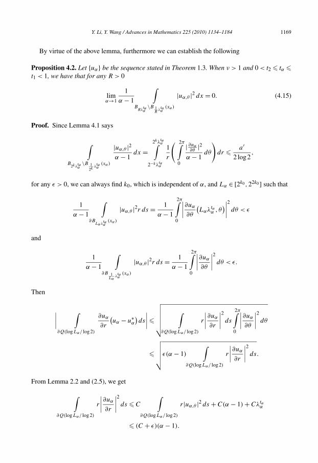
By virtue of the above lemma, furthermore we can establish the following
Proposition 4.2. Let {uα} be the sequence stated in Theorem 1.3. When ν > 1 and 0 < t2 � tα �t1 < 1, we have that for any R > 0
limα→1
1
α − 1
∫B
Rλtαα
\B 1R
λtαα
(xα)
|uα,θ |2 dx = 0. (4.15)
Proof. Since Lemma 4.1 says
∫B
2kλtαα
\B 12k
λtαα
(xα)
|uα,θ |2α − 1
dx =2kλ
tαα∫
2−kλtαα
1
r
( 2π∫0
| ∂uα
∂θ|2
α − 1dθ
)dr � a′
2 log 2,
for any ε > 0, we can always find k0, which is independent of α, and Lα ∈ [2k0 ,22k0 ] such that
1
α − 1
∫∂B
Lαλtαα
(xα)
|uα,θ |2r ds = 1
α − 1
2π∫0
∣∣∣∣∂uα
∂θ
(Lαλtα
α , θ)∣∣∣∣
2
dθ < ε
and
1
α − 1
∫∂B 1
Lαλtαα
(xα)
|uα,θ |2r ds = 1
α − 1
2π∫0
∣∣∣∣∂uα
∂θ
∣∣∣∣2
dθ < ε.
Then
∣∣∣∣∫
∂Q(logLα/ log 2)
∂uα
∂r
(uα − u∗
α
)ds
∣∣∣∣�√√√√√√
∫∂Q(logLα/ log 2)
r
∣∣∣∣∂uα
∂r
∣∣∣∣2
ds
2π∫0
∣∣∣∣∂uα
∂θ
∣∣∣∣2
dθ
�
√√√√√ε(α − 1)
∫∂Q(logLα/ log 2)
r
∣∣∣∣∂uα
∂r
∣∣∣∣2
ds.
From Lemma 2.2 and (2.5), we get
∫∂Q(logLα/ log 2)
r
∣∣∣∣∂uα
∂r
∣∣∣∣2
ds � C
∫∂Q(logLα/ log 2)
r|uα,θ |2 ds + C(α − 1) + Cλtαα
� (C + ε)(α − 1).
1170 Y. Li, Y. Wang / Advances in Mathematics 225 (2010) 1134–1184
By (4.8) and (4.10), we get
(1 − 2ε1)
∫B
Lαλtαα
\B 1Lα
λtαα
(xα)
|∇0uα|2 dx
� ε1(α − 1) + 2(α − 1)(2H(λtα
α
)logLα + ε
). (4.16)
Noting (4.10) we can infer from (2.8)
1
α − 1
∫B
Lαλtαα
\B 1Lα
λtαα
(xα)
(∣∣∣∣∂uα
∂r
∣∣∣∣2
− |uα,θ |2)
dx =Lαλ
tαα∫
1Lα
λtαα
2
rH(r) dr,
which implies that
1
α − 1
∫B
Lαλtαα
\B 1Lα
λtαα
(xα)
(∣∣∣∣∂uα
∂r
∣∣∣∣2
− |uα,θ |2)
dx � 4 logLα
(H(λtα
α
)− ε).
Combining (4.16) with the above inequality we conclude the following inequality holds true asα is close to 1 sufficiently
1
α − 1
∫B
Lαλtαα
\B 1Lα
λtαα
(xα)
|uα,θ |2 dx � ε1 + Cε.
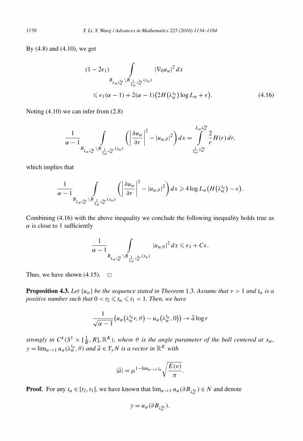
Thus, we have shown (4.15). �Proposition 4.3. Let {uα} be the sequence stated in Theorem 1.3. Assume that ν > 1 and tα is apositive number such that 0 < t2 � tα � t1 < 1. Then, we have
1√α − 1
(uα
(λtα
α r, θ)− uα
(λtα
α ,0))→ �a log r
strongly in Ck(S1 × [ 1R
,R],RK), where θ is the angle parameter of the ball centered at xα ,
y = limα→1 uα(λtαα , θ) and �a ∈ TyN is a vector in R
K with
|�a| = μ1−limα→1 tα
√E(v)
π.
Proof. For any tα ∈ [t2, t1], we have known that limα→1 uα(∂Bλ
tαα
) ∈ N and denote
y = uα(∂B tα ).
λα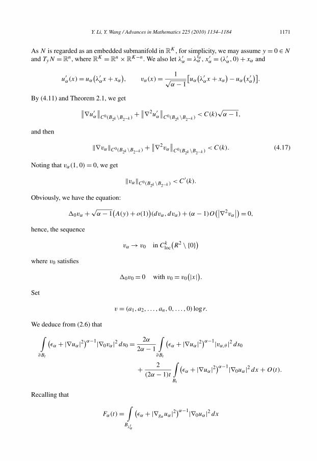
Y. Li, Y. Wang / Advances in Mathematics 225 (2010) 1134–1184 1171
As N is regarded as an embedded submanifold in RK , for simplicity, we may assume y = 0 ∈ N
and TyN = Rn, where R
K = Rn × R
K−n. We also let λ′α = λ
tαα , x′
α = (λ′α,0) + xα and
u′α(x) = uα
(λ′
αx + xα
), vα(x) = 1√
α − 1
[uα
(λ′
αx + xα
)− uα
(x′α
)].
By (4.11) and Theorem 2.1, we get∥∥∇u′α
∥∥C0(B2k \B2−k )
+ ∥∥∇2u′α
∥∥C0(B2k \B2−k )
< C(k)√
α − 1,
and then
‖∇vα‖C0(B2k \B2−k ) + ∥∥∇2vα
∥∥C0(B2k \B2−k )
< C(k). (4.17)
Noting that vα(1,0) = 0, we get
‖vα‖C0(B2k \B2−k ) < C′(k).
Obviously, we have the equation:
�0vα + √α − 1
(A(y) + o(1)
)(dvα, dvα) + (α − 1)O
(∣∣∇2vα
∣∣)= 0,
hence, the sequence
vα → v0 in Ckloc
(R2 \ {0})
where v0 satisfies
�0v0 = 0 with v0 = v0(|x|).
Set
v = (a1, a2, . . . , an,0, . . . ,0) log r.
We deduce from (2.6) that
∫∂Bt
(εα + |∇uα|2)α−1|∇0vα|2 ds0 = 2α
2α − 1
∫∂Bt
(εα + |∇uα|2)α−1|vα,θ |2 ds0
+ 2
(2α − 1)t
∫Bt
(εα + |∇uα|2)α−1|∇0uα|2 dx + O(t).
Recalling that
Fα(t) =∫
B t
(εα + |∇gαuα|2)α−1|∇0uα|2 dx
λα
1172 Y. Li, Y. Wang / Advances in Mathematics 225 (2010) 1134–1184
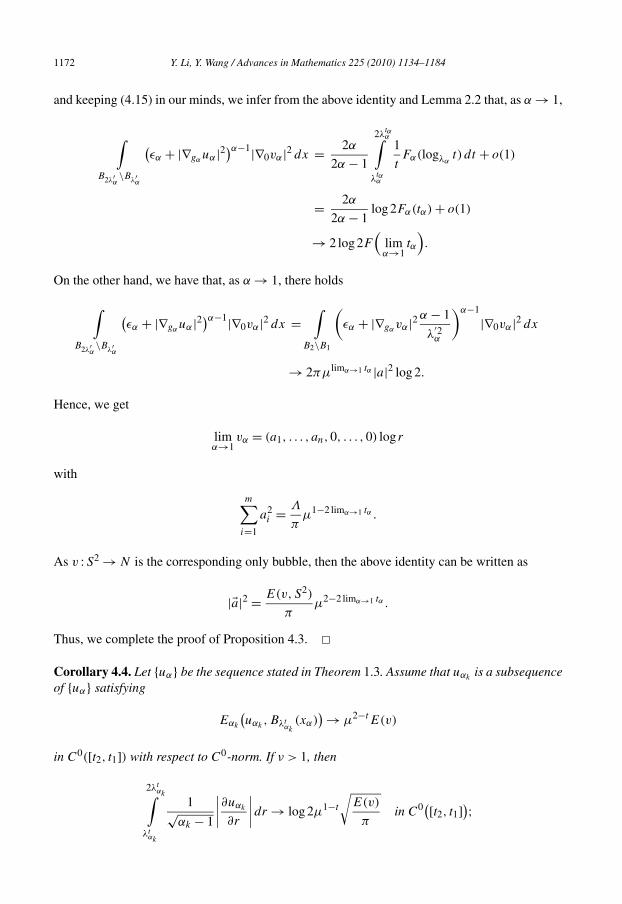
and keeping (4.15) in our minds, we infer from the above identity and Lemma 2.2 that, as α → 1,
∫B2λ′
α\Bλ′
α
(εα + |∇gαuα|2)α−1|∇0vα|2 dx = 2α
2α − 1
2λtαα∫
λtαα
1
tFα(logλα
t) dt + o(1)
= 2α
2α − 1log 2Fα(tα) + o(1)
→ 2 log 2F(
limα→1
tα
).
On the other hand, we have that, as α → 1, there holds
∫B2λ′
α\Bλ′
α
(εα + |∇gαuα|2)α−1|∇0vα|2 dx =
∫B2\B1
(εα + |∇gαvα|2 α − 1
λ′2α
)α−1
|∇0vα|2 dx
→ 2πμlimα→1 tα |a|2 log 2.
Hence, we get
limα→1
vα = (a1, . . . , an,0, . . . ,0) log r
with
m∑i=1
a2i = Λ
πμ1−2 limα→1 tα .
As v :S2 → N is the corresponding only bubble, then the above identity can be written as
|�a|2 = E(v,S2)
πμ2−2 limα→1 tα .
Thus, we complete the proof of Proposition 4.3. �Corollary 4.4. Let {uα} be the sequence stated in Theorem 1.3. Assume that uαk
is a subsequenceof {uα} satisfying
Eαk
(uαk
,Bλtαk
(xα))→ μ2−tE(v)
in C0([t2, t1]) with respect to C0-norm. If ν > 1, then
2λtαk∫
λt
1√αk − 1
∣∣∣∣∂uαk
∂r
∣∣∣∣dr → log 2μ1−t
√E(v)
πin C0([t2, t1]);
αk
Y. Li, Y. Wang / Advances in Mathematics 225 (2010) 1134–1184 1173
and
1√αk − 1
(r
∣∣∣∣∂uαk
∂r
∣∣∣∣)(
λtαk
, θ)→ μ1−t
√E(v)
πin C0([t2, t1]).
Proof. We need only to prove the first claim, since the proof of the second claim is similar. Ifthe first claim was not true, then we assumed that there was a subsequence αki
, ti → t0 such that
∣∣∣∣∣2λ
tiαki∫
λtiαki
1√αki
− 1
∣∣∣∣∂uαki
∂r
∣∣∣∣dr − log 2μ1−ti
√E(v)
π
∣∣∣∣∣� ε > 0.
On the other hand, from the above arguments on Proposition 4.3 we know that, after passingto a subsequence, there holds
uαki(λαki
x) − uαki(λαki
,0)√αki
− 1→ �a log r,
with |�a| = |μ1−t0
√E(v)
π|. Hence we derive the following
limi→+∞
2λtiαki∫
λtiαki
1√αki
− 1
∣∣∣∣∂uαki
∂r
∣∣∣∣dr = |�a|2∫
1
1
rdr = log 2μ1−t0
√E(v)
π.
This is a contradiction. �4.2.2. The neck is a geodesic
To show the neck for the α-harmonic map sequence is just a geodesic in N which joins N andthe bubble, we define the following curve
ωα(r) ≡ 1
2π
2π∫0
uα(r, θ) dθ :[λt1
α ,λt2α
]→ RK,
which is denoted by Γα . From (4.6), it is easy to see that for any rk → 0, ωα(rk) converges to apoint p ∈ N after passing to a subsequence. Moreover, for any fixed R, it is easy to see ωα(r)
converges to the point p in [ 1R
rk,Rrk] as rk → 0. However, if we use the arc length of each curveΓα to parameterize the curve ωα , then we will see that ωα(·) converges locally. For the sake ofconvenience, sometimes we denote the derivatives ∂f (r,θ)
∂rand ∂f (r,θ)
∂θof f (r, θ) by f and f ,θ
respectively.
1174 Y. Li, Y. Wang / Advances in Mathematics 225 (2010) 1134–1184
By computation we have
ωα = 1
2π
2π∫0
uα(r, θ) dθ = 1
2π
2π∫0
(uα(r, θ) + uα,θθ
r2
)dθ
= 1
2π
2π∫0
�0uα dθ − 1
2π
2π∫0
uα
rdθ
= − 1
2π
2π∫0
A(uα)(duα, duα) − α − 1
2π
2π∫0
∇0|∇guα|2∇0uα
ε2α + |∇guα|2 dθ − ωα
r,
where we have used the fact∫ 2π
0 uα,θθ (r, θ) dθ = 0.In order to prove Γα converges to a geodesic we need to analyze the asymptotic behavior of
Γα as α → 1. By virtue of Proposition 4.3, we can derive the following the asymptotic estimateson the metric and the second fundamental form of Γα .
Lemma 4.5. Denote the induced metric of Γα in RK by hα , and the second fundamental form
by AΓα . Then, after passing to a subsequence, for λtαα ∈ [λt1
α ,λt2α ] there holds
ωα
(λtα
α
)=√
α − 1
λtαα
(�a + o(1)),
hα
(d
dr,
d
dr
)= |ωα|2 = α − 1
λ2tαα
(|�a|2 + o(1)); (4.18)
and
AΓα(dωα, dωα) = α − 1
λ2tαα
(A(y)(�a, �a) + o(1)
). (4.19)
Moreover, for any t ∈ [t2, t1] there exists a constant such that
‖AΓα‖2hα
(λt
α
)< C.
Proof. Let
Gα = −ωα − ωα
r.
Given λtαα ∈ [λt1
α ,λt2α ]. As before, we always have
uα(λtαα r, θ) − uα(λ
tαα ,0)√ → �a log r,
α − 1
Y. Li, Y. Wang / Advances in Mathematics 225 (2010) 1134–1184 1175
where �a ∈ TyN and y = limα→1 uα(λtαα , θ). Therefore, we have
ωα
(λtα
α
)=√
α − 1
λtαα
(�a + o(1)), hα
(d
dr,
d
dr
)= |ωα|2 = α − 1
λ2tαα
(|�a|2 + o(1)),
where o(1) → 0 as α → 1. Moreover, we have
Gα
(λtα
α
)= 1
2π
2π∫0
A(uα)(duα, duα) dθ + α − 1
2π
2π∫0
∇0|∇gαuα|2∇0uα
ε2α + |∇gαuα|2 dθ
= α − 1
λ2tαα
(1
2π
2π∫0
A(y)(�a, �a)dθ + o(1)
)+ (α − 1)
2π∫0
O(∣∣∇2
gαuα
∣∣)dθ
= α − 1
λ2tαα
(1
2π
2π∫0
A(y)(�a, �a)dθ + o(1) + √α − 1
2π∫0
O
(λ
2tαα |∇2
gαuα|√
α − 1
)dθ
)
= α − 1
λ2tαα
(1
2π
2π∫0
A(y)(�a, �a)dθ + o(1) + √α − 1
2π∫0
O(∣∣∇2
gαvα
∣∣)dθ
)
= α − 1
λ2tαα
(A(y)(�a, �a) + o(1) + O
(√α − 1
))
= α − 1
λ2tαα
(A(y)(�a, �a) + o(1)
),
where we have used estimate (4.17) on vα defined in the proof of Proposition 4.3, and have alsomade use of the fact ν > 1 which implies that for any m > 0
λ2tαα = o
((α − 1)m
).
Noting that 〈A(y)(�a, �a), �a〉 = 0, we get
−AΓα(dωα, dωα) = ωα − 〈ωα, ωα〉|ω|2 ωα = −Gα + 〈Gα, ωα〉ωα
|ωα|2
= −α − 1
λ2tαα
(A(y)(�a, �a) + o(1)
).
Hence, we conclude ‖AΓα‖2hα
(λtαα ) < C. Similar to the proof of Corollary 4.4, after passing to a
subsequence we have that for any t ∈ [t2, t1],‖AΓα‖2
hα
(λt
α
)< C. �
Proposition 4.6. Assume that {uα} be the sequence stated in Theorem 1.3. Then, after passing to asubsequence, the curve sequence Γα in R
K , each of which is defined by ωα(r) and parameterizedby its arc length, converges to a geodesic on (N,h) as α tends to 1.
1176 Y. Li, Y. Wang / Advances in Mathematics 225 (2010) 1134–1184
Proof. For every ωα we fix
yα = ωα
(λtα
α
)= 1
2π
2π∫0
uα
(λtα
α , θ)dθ,
and let s be the arc length parameter of ωα(t) with s(λtαα ) = 0. We know that the sequence of
points {ωα(λtαα )} is convergent as α → 1. Denote y = limα→1 yα . It is well known that the norm
of the second fundamental form ‖AΓα‖2hα
does not depend on the choice of parameter, and
d2ωα
ds2= −AΓα(ωα)
(dωα
ds,dωα
ds
),
then ωα(s) converges locally to a smooth vector value function from [0, s1] into RK , denoted
by ω(s), in C1, where s1 is sufficiently small and s is still the arc length parameter. This impliesthat Γα|[λt1
α ,λt2α ] converges locally to a curve Γ .
The remaining part of proof is to prove Γ is a geodesic on N . To verify Γ satisfies geodesicequation, it is crucial to show
AΓα(ωα)
(dωα
ds,dωα
ds
)→ A(ω)
(dω
ds,dω
ds
)(4.20)
strongly in C0([0, s1],RK), where A(·)(·,·) is the second fundamental form of N as a submani-
fold in RK . We claim that the above convergence is true. If this was not true, then for any small
s1 we could find a subsequence of {uα}, still denoted by {uα}, such that
s′α =
λt ′αα∫
λtαα
|ωα|dr → s′ ∈ (0, s1),
and ∣∣∣∣AΓα(ωα)
(dωα
ds,dωα
ds
)− A(ω)
(dω
ds,dω
ds
)∣∣∣∣s=s′
α
> ε.
We can always choose a small enough s1 such that, when s′α < s1 and α − 1 is small enough,
the corresponding t ′α ∈ [ t22 , t1]. This is implied by Corollary 4.4. For simplicity, we may assume
λt22α = 2P λtα
α
where P is an integer. Indeed, applying Corollary 4.4 we have
2i+1λtαα∫
i tα
|ωα|dr = √α − 1μ1−(tα−i logλα
2)
(log 2
√E(v)
π+ oα(1)
).
2 λα
Y. Li, Y. Wang / Advances in Mathematics 225 (2010) 1134–1184 1177
Therefore, as α is close to 1 enough,
λ
t22
α∫λ
tαα
|ωα|dr =P−1∑i=0
2i+1λtαα∫
2iλtαα
|ωα|dr � P√
α − 1
(√E(v)
πlog 2 + oα(1)
)
� C
(tα − t2
2
)logλ−√
α−1α
� Ct2
2logν > 0.
Therefore, we may always pick s1 to be very small, for example s1 < C t22 logν, such that t ′α ∈
[ t22 , t1] as α − 1 is small enough.
Since t ′α ∈ [ t22 , t1], by applying Proposition 4.3 we have
uα(λt ′αα r, θ) − uα(λ
t ′αα ,0)√
α − 1→ �a′ log r.
Obviously,
ωα(λt ′αα )
|ωα(λt ′αα )|
= dωα
ds
(s′α
)→ dω
ds
(s′).
Applying (4.18) and (4.19) in Lemma 4.5 with t ′α instead of tα , we know that, after passing to asubsequence, the following holds
AΓα(ωα)
(dωα
ds,dωα
ds
)∣∣∣∣s=s′
α
= 1
|ωα(λt ′αα )|2
AΓα(ωα)(ωα, ωα)|r=λ
t ′αα
→ A(ω)
(dω
ds,dω
ds
)∣∣∣∣s=s′
which contradicts the choice of s′α . Thus, the assertion (4.20) is proved.
So, we infer from the curve equation of ωα and the fact (4.20) that the following
dω
ds(s) − dω
ds(0) = −
s∫0
A(ω)
(dω
ds,dω
ds
)ds
holds true in interval [0, s1]. This shows ω is smooth near 0 and satisfies in [0, s1]d2ω
ds2= −A(ω)
(dω
ds,dω
ds
).
Therefore, we obtain
∇Ndωds
dω
ds= d2ω
ds2+ A(ω)
(dω
ds,dω
ds
)= 0,
which means that Γ is a geodesic. Thus we complete the proof of this proposition. �
1178 Y. Li, Y. Wang / Advances in Mathematics 225 (2010) 1134–1184
4.2.3. The proofs of Theorem 1.3 for the case ν > 1 and Corollary 1.5Next, we give the length formula of the neck, i.e. calculate the length of the geodesic Γ .
Proof of Theorem 1.3 for the case ν > 1. By Proposition 4.6 we have known that the neckconverges to a geodesic. We only need to calculate the length of the geodesic. Without loss ofgenerality, as before we may assume λ
t2α = 2P λ
t1α for some integer P . Then we have
P = t2 − t1
log 2logλα.
When ν = +∞, by Corollary 4.4, we have
L(Γα|B2k+1λ
t1α \2kλ
t1α
(xα)) �√
α − 1
(√E(v)
πlog 2 + o(1)
).
Then,
L(Γα) � CP√
α − 1 � C logλ−√α−1
α → +∞.
This implies
L(Γ ) = +∞.
Now, we assume ν < +∞. By Corollary 4.4,
L(Γα|B2k+1λ
t1α \2kλ
t1α
(xα)) = √α − 1
(√E(v)
πlog 2 + oα(1)
),
where oα(1) → 0 as α → 1 uniformly. Hence
L(Γ ) = limα→1
√α − 1P
√E(v)
πlog 2 = (t1 − t2)
√E(v)
πlogν.
Now, it is easy to see that to complete the proof of Theorem 1.3 we only need to prove thefollowing:
oscBλtα\BRλα (xα) uα → 0, as α → 1, then R → +∞ and t → 1; (4.21)
and
oscBδ\Bλtα(xα) uα → 0, as α → 1, then δ → 0 and t → 0. (4.22)
Since ν < +∞ implies μ = 1, from Theorem 1.1 we know
limt→1
limR→+∞ lim
α→1
∫B t \BRλα (xα)
|∇uα|2 = 0.
λα
Y. Li, Y. Wang / Advances in Mathematics 225 (2010) 1134–1184 1179
Therefore, we can use the same method as in Section 4.1 (we replace δ with λtα) to deduce
oscBλtα\BRλα
uα � C
√E(uα,Bλt
α\ BRλα (xα)
)+ C(1 − t) logν + C√
α − 1,
then (4.21) follows. Similarly, we can prove (4.22). Hence, we derive the length formula of thegeodesic Γ
L =√
E(v)
πlogν.
Thus, we finish the proof of Theorem 1.3. �Remark 4.7. Although we state and prove Theorem 1.3 only for one bubble case, it is not difficultto follow the steps in Section 3.2 to prove the general case. However, the general case is quitecomplicated, for example, if we have 2 bubbles: uα(λ1
αx + x1) → v1, and uα(λ2αx + x1) → v2
which satisfy: λ1α/λ2
α → 0 and ν1, ν2 < ∞, then u0(Bδ(x1)), v2(S2) are connected by a geodesicwith length
L =√
E(v1) + E(v2)
πlogν2,
v1(S2) and v2(S2) are connected by a geodesic of length
L =√
E(v1)
πlog
ν1
ν2.
Proposition 4.8. If ν < +∞, then when (α − 1) is sufficiently small, all the uα belong to ahomotopy class.
Proof. When αi − 1 and αj − 1 are sufficiently small, we have ‖ui −uj‖C0 � i(N) where i(N)
is the injective radius of N . Hence, by using exponential map we know that uαiand uαj
arehomotopic in M \ Bδ , B
λt2α
\ Bλ
t1α
and BRλα respectively.Let p = u0(0) and q = v(+∞). By (4.21), we know that ui(Bδ(xα) \ B
λt2α(xα)) is contained
in a simply connected ball centered at p when α is close to 1 enough, δ and t2 are small enough.Similarly, by (4.22) we also have uj (Bλ
t1α
\ BRλα (xα)) is contained in a small simply connectedball in N with center q when α − 1, δ and 1 − t1 are sufficiently small. Hence ui and uj arehomotopic in Bδ \ B
λt2α
and Bλ
t1α
\ BRλα respectively. So ui and uj are homotopic. �Proof of Corollary 1.5. Corollary 1.5 follows directly from the above proposition. �5. Some comments and an example
In this paper we only consider the case {uα} (α → 1) is a sequence of α-harmonic maps froma closed compact Riemann surface the conformal structure of which is fixed. Naturally, one willask the following problems: (i) What can we say in the case uα is a sequence of α-harmonic maps
1180 Y. Li, Y. Wang / Advances in Mathematics 225 (2010) 1134–1184
and the conformal structure of M varies with α? (ii) Can the methods in this paper be extendedto a class of variational problems which are more general than α-energy? In a forthcoming paperwe will further develop some tools to discuss some issues which relate to the above problems.
On the other hand, one want to know whether one can give an example of a sequence of α-harmonic maps to show there is a neck joining the bubbles which is of infinite length or not.However, if we can construct a manifold N and find a minimizing α-harmonic map sequencewhich satisfies the conditions of Corollary 1.5, then the corollary tells us that, indeed, thereexists a neck which is of infinite length. By modifying the example given by Duzaar and Kuwert(see p. 304 of [8]) we can construct such example as follows:
Example. Let Z3 act on R
3 by τκ(x, y, z) = (x + 4k1, y + 4k2, z + 4k3), whereκ = (k1, k2, k3) ∈ Z
3. Consider
X = R3 \⋃κ
τκ
(B1(0)
).
Let X be the quotient space of X modulo Z3. Obviously, X is a compact manifold with boundary.
Topologically, X is T3 minus a small ball.
Let Φ be a smooth map from R2 to ∂B1(0) satisfying
Φ(x) ={
(1,0,0), |x| > 2,
(−1,0,0), |x| < 1;
and the degree of map Φ denoted by deg(Φ) is 1 if we consider Φ as a map from S2 to S2,i.e. deg(Φ) = 1. Moreover, we let γk : [0,1] → X be a curve which connects (4k + 1,0,0) and(−1,0,0) with γ (1) = (−1,0,0) and ‖γk‖L∞ � 8k. For δ � 1 and R � 2 we define
vk =
⎧⎪⎨⎪⎩
Φ(x), |x| � δ,
γk(log |x|−logRεk
log δ−logRεk), Rεk < |x| < δ,
τ(k,0,0)(Φ( xεk
)), |x| � Rεk.
Denote the projection from X to X by Π , then Π(vk) ∈ π2(X). It is easy to verify
∫Bδ\BRεk
|∇vk|2 = 2π
δ∫Rεk
∣∣∣∣∂γk
∂r
∣∣∣∣2
r dr
<c‖γk‖2
L∞(log δ − log(Rεk))2
δ∫Rεk
dr
r= c‖γk‖2
L∞log δ − log(Rεk)
,
∫2
|∇vk|2 � E(Φ), and∫
B
|∇vk|2 � E(Φ).
R \Bδ Rεk
Y. Li, Y. Wang / Advances in Mathematics 225 (2010) 1134–1184 1181
So, we can choose suitably εk such that
E(Π(vk)
)= E(vk) � 2E(Φ) + 1.
We claim that [Π(vk)] are some homotopy classes which are different from each other. If thiswas not true, we could find a continuous map
H(x, t) :S2 × [0,1] → X
such that
H(x,0) = Π(vi) and H(x,1) = Π(vj ).
Since S2 ×[0,1] is simply connected, we are able to lift H to H which is a map from S2 ×[0,1]into X with H (x,0) = vi . We assume that H (x,1) = τκ(vj ). Hence [vi] = [τκ(vj )]. Therefore,
[∂B1(0) + γi + ∂τ(i,0,0)
(B1(0)
)]= [∂τκ
(B1(0)
)+ τκγj + ∂τκτ(j,0,0)
(B1(0)
)]in π2(X),
where π2(X) is the second homotopy group of X. However, it is easy to check that π1(X) = {1},then by Hurewicz Theorem, the above identity is not true.
Now, we construct the target manifold N in the following way: Let f be a homeomorphismfrom X to Y = X. We consider the quotient space of X ∪ Y , obtained by gluing every pointx ∈ ∂X with f (x) ∈ ∂Y together. Thus, we get a closed compact manifold N and a projectionφ :N → X. One is easy to check that Π(vk) can be also considered as a map from S2 to N withE(Π(vk)) < C. It is easy to check that [Π(vk)] are some homotopy classes which are differentfrom each other in π2(N). Indeed, if it was not true. Then, we could find a continuous mapH(x, t) :S2 × [0,1] → N such that H(x,0) = Π(vi) and H(x,1) = Π(vj ). Hence, φ(H(x, t))
was just a homotopic map of Π(vi) and Π(vj ) in X. This is a contradiction.Let uαk
:S2 → N be the minimizer of Eαk(u) in [Π(vk)], where αk → 1. It is easy to see
{uαk} is a sequence of α-harmonic maps which satisfies the assumptions in Corollary 1.5. We
conclude that {uαk} blows up certainly at some points in S2 and there exists at least a geodesic
of infinite length in the limiting set of {uαk}.
Finally, we would like to ask the following problems:
Problem 1. Suppose all α-harmonic maps uα belong to the same homotopy class and satisfy theenergy identity as α → 1. Do the necks consist of some geodesics of finite length?
Problem 2. Could we find a sequence of αk-harmonic maps uαk(αk → 1) such that (1) the Morse
index tends to infinite; (2) supk Eαk(uαk
) < ∞; (3) for any i = j , uαiand uαj
are not homotopicto each other.
Acknowledgments
The authors are grateful to Prof. Weiyue Ding for his help and encouragement, and the refereefor his beneficial suggestions which make the paper more readable. The first author would alsolike to thank Prof. Ernst Kuwert for many helpful discussions.
1182 Y. Li, Y. Wang / Advances in Mathematics 225 (2010) 1134–1184
Appendix A
In this section we demonstrate how to construct the bubble trees at every energy concentrationpoint of a sequence of α-harmonic maps.
Assume that uα ∈ C∞(Bσ ,N) is the sequence stated in Theorem 1.1. Denote by S(uα,B) theset {
x ∈ Bσ : limα→1
lim infr→0
∫Br(x)
|∇0uα|2 dx >ε0
2
},
where ε0 is the constant defined in Theorem 2.1. Usually, S(uα,Bσ ) is called the set of energyconcentration points (or simply concentration points) for {uα} on Bσ . Obviously, S(uα,Bσ ) is afinite set. One is easy to see that for any x /∈ S(uα,Bσ ), there holds∫
Br(x)
|∇0uα|2 dx < ε0,
for sufficiently small r and α − 1. So, for any Ω ⊂ Bσ \ S(uα,Bσ ), there exists a subsequenceof {uα} which converges in Ω .
Now, we show how to construct the bubble trees at each concentration point of S(uα,Bσ ).For simplicity we assume 0 is the only concentration point for {uα}.
Step 1. Set r1α = λ1
α = 1maxBσ/2 |uα | . Let maxBσ/2 |uα| be attained at the point x1
α . Since uα
converges smoothly away the concentration point, we have x1α → 0. Let v1
α = uα(x1α + λ1
αx).Obviously, ‖∇v1
α‖L∞ = 1. Hence, v1α converges to a harmonic map v1 from R
2 to N locally andsmoothly. As |∇v1(0)| = 1, we know that v1 is not trivial. We call v1 is the first bubble.
Step 2. To find the second bubble, we need to consider the following two cases.
Case 1. If for any ε > 0, we can find a positive number δ0 and a positive R such that∫B2ρ\Bρ(x1
α)
|∇uα|2 < ε (A.1)
holds for any ρ ∈ [Rr1α, δ0], then energy concentration phenomena disappears. This means that
there is only one bubble for the sequence {uα}.
Case 2. If (A.1) is not true, then we can find r2α → 0 such that limα→1
r2α
r1α
= +∞, and
∫B
2r2α\B
r2α(x1
α)
|∇uα|2 > ε1 > 0, (A.2)
i.e. there are still some points where energy concentration happens. We set u2α = uα(x1
α + r2αx),
and denote the set of energy concentration points of {u2 } on R2 by S(u2 ,R
2). Obviously,
α α
Y. Li, Y. Wang / Advances in Mathematics 225 (2010) 1134–1184 1183
0 ∈ S(u2α,R
2), and v1 is also a bubble for the sequence {u2α}. Moreover, passing to a subse-
quence we have u2α converges to a harmonic map u2
0 away from S 2(u2α,R
2), where u20 is a
harmonic map from R2 into N . Then we have two cases: (a) u2
0 is trivial, i.e. a constant map;(b) u2
0 is a non-trivial harmonic map from R2 to N .
If u20 is trivial, (A.2) implies that S 2(u2
α,R2) ∩ (B3 \ B1/2) = ∅, i.e. there must exist another
concentration point p for u2α lies in B3 \ B1/2. At this new point of energy concentration for
{u2α}, we can get a bubble for {u2
α} by the same program as in Step 1. That is to say, we may findx′α → p and λ′
α → 0 such that
u2α
(x′α + λ′
αx)→ v2,
where v2 is a harmonic map from R2 to N . If we set x2
α = x′α + λ1
αx1α , λ2
α = λ1αλ′
α , we get
uα
(x2α + λ2
αx)→ v2,
therefore, v2 is also a bubble for the sequence uα . Next, we repeat Step 1 and then repeat Step 2at each concentration point for {u2
α}.When u2
0 is non-trivial, v2 = u20 is a harmonic map from R
2 to N . v2 is regarded as the secondbubble. At each point of S 2(u2
α,R2), we repeat Step 1, and then repeat Step 2.
Step 3. We replace r1α in Step 1 with r2
α and continue Step 2 again.
In this way, we can get xkα → 0, λk
α → 0 such that
uα
(xkα + λk
αx)→ vk, k = 1,2, . . . ,m,
where vk are harmonic maps from R2 to N . One is easy to check that for any i = j one of the
(H1) and (H2) always hold. Moreover, since
∫Bσ
(εα + |∇uα|2)α dVg �
m∑i=1
∫S2
∣∣∇vi∣∣2,
our procedure of construction must stop after finite steps, i.e. we can find a sequence of rk0α such
that for any ε > 0, there exist δ0 and R such that for any λ ∈ [Rrk0α , δ0]∫
B2λ\Bλ
|∇uα|2 < ε. (A.3)
References
[1] K.C. Chang, Heat flow and boundary value problem for harmonic maps, Ann. Inst. H. Poincaré Anal. NonLinéaire 6 (5) (1989) 363–395.
[2] K.C. Chang, W.Y. Ding, R. Ye, Finite time blow-up of the heat flow of harmonic maps from surfaces, J. DifferentialGeom. 36 (1992) 507–515.
[3] J. Chen, G. Tian, Compactification of moduli space of harmonic mappings, Comment. Math. Helv. 74 (1999) 201–237.
1184 Y. Li, Y. Wang / Advances in Mathematics 225 (2010) 1134–1184
[4] T.H. Colding, W.P. Minicozzi II, Width and finite extinction time of Ricci flow, Geom. Topol. 12 (2008) 2537–2586.[5] W. Ding, Lectures on the heat flow of harmonic maps, manuscript.[6] W. Ding, Blow-up of solutions of heat flows for harmonic maps, Adv. Math. (China) 19 (1) (1990) 80–92.[7] W. Ding, G. Tian, Energy identity for a class of approximate harmonic maps from surfaces, Comm. Anal. Geom. 3
(1995) 543–554.[8] F. Duzaar, E. Kuwert, Minimization of conformally invariant energies in homotopy classes, Calc. Var. Partial Dif-
ferential Equations 6 (1998) 285–313.[9] J. Eells, J.H. Sampson, Harmonic mappings of Riemannian manifolds, Amer. J. Math. 86 (1964) 109–160.
[10] J. Jost, Two-dimensional Geometric Variational Problems, John Wiley and Sons, Chichester, 1991.[11] T. Lamm, Energy identity for approximations of harmonic maps from surfaces, Trans. Amer. Math. Soc., in press.[12] Y. Li, Y. Wang, Bubbling location for a sequence of approximate f -harmonic maps from surfaces, Internat. J. Math.,
in press.[13] F. Lin, C. Wang, Energy identity of harmonic map flows from surfaces at finite singular time, Calc. Var. Partial
Differential Equations 6 (1998) 369–380.[14] J.D. Moore, Energy growth in minimal surface bubbles, http://www.math.ucsb.edu/~moore/growthrev.pdf.[15] J. Qing, On singularities of the heat flow for harmonic maps from surfaces into spheres, Comm. Anal. Geom. 3
(1995) 297–315.[16] J. Qing, G. Tian, Bubbling of the heat flow for harmonic maps from surfaces, Comm. Pure Appl. Math. 50 (1997)
295–310.[17] J. Sacks, K. Uhlenbeck, The existence of minimal immersions of 2-spheres, Ann. of Math. 113 (1981) 1–24.[18] M. Struwe, On the evolution of harmonic maps of Riemannian surfaces, Comment. Math. Helv. 60 (1985) 558–581.[19] P. Topping, Winding behaviour of finite-time singularities of the harmonic map heat flow, Math. Z. 247 (2004)
279–302.


![arXiv:1904.05800v1 [math.AP] 11 Apr 20194 ANUDEEP K. ARORA Remark 1.2. Their result also contains the finite time blow-up conclusion in the case when ku0kL2k∇u0kL2 > kQkL2k∇QkL2,](https://static.fdocument.org/doc/165x107/5fda6aa82b5d295dc855a7c6/arxiv190405800v1-mathap-11-apr-2019-4-anudeep-k-arora-remark-12-their-result.jpg)