A Suite of Models for Dynare - fabcol.free.frfabcol.free.fr/dynare/pdf/models.pdf · A Suite of...

A Suite of Models for DynareDescription of Models

F. Collard, H. Dellas and B. Diba Version 1.0

Department of Economics University of Bern

1 A REAL BUSINESS CYCLE MODEL 2

1 A real Business Cycle Model

The problem of the household is

max Et

∞∑j=0

βj

ζ 1σc,t+j

c1− 1

σt+j

1− 1σ

− ψ

1 + νζ−νh,t+jh

1+νt+j

ct + it = wtht + ztkt − τtkt+1 = it + (1− δ)kt

The last two conditions can be combined to give

kt+1 = wtht + (zt + 1− δ)kt − ct − τtThen the first order conditions are given by

ζ1σc,tc− 1σ

t = λt (1)

ψζ−νh,t hνt = λtwt (2)

λt = βEt (λt+1(zt+1 + 1− δ)) (3)

The problem of the firm ismax atk

αt h

1−αt − wtht − ztkt

which leads to the first order conditions

wt = (1− α)ytht

and zt = αytkt

The taxes, τt, finance an exogenous stream of government expenditures, gt, such that τt = gt.

All shocks follow AR(1) processes of the type

log(at+1) = ρa log(at) + εa,t+1

log(gt+1) = ρg log(gt) + (1− ρg) log(g) + εg,t+1

log(ζc,t+1) = ρc log(ζc,t) + εc,t+1

log(ζh,t+1) = ρh log(ζh,t) + εh,t+1

The general equilibrium is therefore represented by the following set of equations

ζ1σc,tc− 1σ

t = λt

ψζ−νh,t hνt = λt(1− α)

ytht

λt = βEt(λt+1(α

yt+1

kt+1+ 1− δ)

)kt+1 = it + (1− δ)ktyt = atk

αt h

1−αt

yt = ct + it + gt

and the definition of the shocks.


2 A NOMINAL MODEL WITH PRICE ADJUSTMENT COSTS 3

2 A Nominal Model with Price Adjustment Costs

In all what follows, we will assume zero inflation in the steady state.

The problem of the household is

max Et

∞∑j=0

βj

ζ 1σc,t+j

c1− 1

σt+j

1− 1σ

− ψ

1 + νζ−νh,t+jh

1+νt+j

Bt + Ptct + Ptit = Rt−1Bt−1Ptwtht + Ptztkt − Ptτtkt+1 = it + (1− δ)kt

The last two conditions can be combined to give

Bt + Ptct + Ptkt+1 = Rt−1Bt−1Ptwtht + Pt(zt + 1− δ)kt − Ptτt

Then the first order conditions are given by

ζ1σc,tc− 1σ

t = ΛtPt (4)

ψζ−νh,t hνt = ΛtPtwt (5)

ΛtPt = βEt (Λt+1Pt+1(zt+1 + 1− δ)) (6)

Λt = βRtEtΛt+1 (7)

The economy is comprised of many sectors. The first sector —the final good sector— combinesintermediate goods to form a final good in quantity yt:

yt =

(∫ 1

0yt(i)

θ−1θ di

) θθ−1

(8)

The problem of the final good firm is then

max{yt(i);i∈(0,1)}

Ptyt −∫ 1

0Pt(i)yt(i)di

subject to (8), which rewrites

max{yt(i);i∈(0,1)}

Pt

(∫ 1

0yt(i)

θ−1θ di

) θθ−1

−∫ 1

0Pt(i)yt(i)di

which gives rise to the demand function

yt(i) =

(Pt(i)

Pt

)−θyt (9)

These intermediate goods are produced by intermediaries, each of which has a local monopolypower. Each intermediate firm i, i ∈ (0, 1), uses a constant returns to scale technology

yt(i) = atkt(i)αht(i)

1−α (10)


2 A NOMINAL MODEL WITH PRICE ADJUSTMENT COSTS 4

where kt(i) and ht(i) denote capital and labor. The firm minimizes its real cost subject to (10).Minimized real total costs are then given by stxt(i) where the real marginal cost, st, is given by

st =zαt w

1−αt

ςat

with ς = αα(1− α)1−α.

Intermediate goods producers are monopolistically competitive, and therefore set prices for thegood they produce. However, it incurs a cost whenever it changes its price relatively to the earlierperiod. This cost is given by

ϕp2

(Pt(i)

Pt−1(i− 1

)2

yt

The problem of the firm is then to maximize the profit function

Et

∞∑j=0

Φt,t+j

(Pt+j(i)yt+j(i)− Pt+jst+jyt+j(i)− Pt+j

ϕp2

(Pt+j(i)

Pt+j−1(i− 1

)2

yt+j

) (11)

where Φt,t+j is an appropriate discount factor derived from the household’s optimality conditions,

and proportional to βj Λt+jΛt

. The first order condition of the problem is given by

(1− θ)(Pt(i)

Pt

)−θyt + θ

PtPt(i)

st

(Pt(i)

Pt

)−θyt −

PtPt−1(i)

ϕp

(Pt(i)

Pt−1(i− 1

)yt

+ βEt[

Λt+1

Λt

Pt+1Pt+1(i)

Pt(i)2ϕp

(Pt+1(i)

Pt(i− 1

)yt+1

]= 0

Using Sheppard’s lemma we get the demand for each input

wt = (1− α)styt(i)

ht(i)

zt = αstyt(i)

kt(i)

The taxes, τt, finance an exogenous stream of government expenditures, gt, such that

τt = gt

In order to close the model, we add a Taylor rule that determines the nominal interest rate

log(Rt) = ρr log(Rt−1) + (1− ρ)(log(R) + γπ(log(πt)− log(π)) + γy(log(yt)− log(y))

)where πt = Pt/Pt−1 denotes aggregate inflation.







3 A NOMINAL MODEL WITH STAGGERED PRICE CONTRACTS 5

The symmetric general equilibrium is therefore represented by the following set of equations

ζ1σc,tc− 1σ

t = λt

ψζ−νh,t hνt = λt(1− α)st

ytht

λt = βEt(λt+1

(αst+1

yt+1

kt+1+ 1− δ

)]λt = βRtEt

(λt+1

πt+1

)0 = (1− θ)yt + θstyt − πtϕp (πt − 1) yt + βEt

[λt+1

λtπt+1ϕp (πt+1 − 1) yt+1

]kt+1 = it + (1− δ)ktyt = atk

αt h

1−αt

yt = ct + it + gt +ϕp2

(πt − 1)2yt


)and the definition of the shocks.

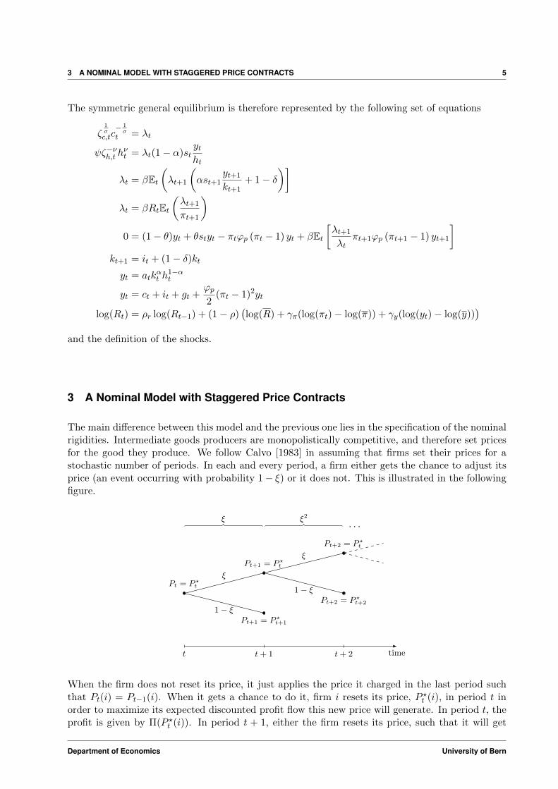
3 A Nominal Model with Staggered Price Contracts

The main difference between this model and the previous one lies in the specification of the nominalrigidities. Intermediate goods producers are monopolistically competitive, and therefore set pricesfor the good they produce. We follow Calvo [1983] in assuming that firms set their prices for astochastic number of periods. In each and every period, a firm either gets the chance to adjust itsprice (an event occurring with probability 1− ξ) or it does not. This is illustrated in the followingfigure.

timet

Pt = P ?t

t+ 1

ξ

1− ξPt+1 = P ?t+1

ξ

Pt+1 = P ?tξ

Pt+2 = P ?t

1− ξPt+2 = P ?t+2

ξ2

t+ 2

. . .

When the firm does not reset its price, it just applies the price it charged in the last period suchthat Pt(i) = Pt−1(i). When it gets a chance to do it, firm i resets its price, P ?t (i), in period t inorder to maximize its expected discounted profit flow this new price will generate. In period t, theprofit is given by Π(P ?t (i)). In period t + 1, either the firm resets its price, such that it will get



Π(P ?t+1(i)) with probability q, or it does not and its t+ 1 profit will be Π(P ?t (i)) with probabilityξ. Likewise in t+ 2. The expected profit flow generated by setting P ?t (i) in period t writes

maxP ?t (i)

Et

∞∑j=0

Φt,t+jξjΠ(P ?t (i))

subject to the total demand it faces:

yt(i) =

(Pt(i)

Pt

)−θyt

and where Π(P ?t (i)) = (P ?t (i)− Pt+jst+j) yt+j(i). Φt,t+j is an appropriate discount factor relatedto the way the household value future as opposed to current consumption, such that

Φt,t+j ∝ βjΛt+jΛt

This leads to the price setting equation

Et

∞∑j=0

(βξ)jΛt+jΛt

((1− θ)

(P ?t (i)

Pt+j

)−θyt+j + θ

Pt+jPt+j(i)

(P ?t (i)

Pt+j

)−θst+jyt+j

) = 0

from which it shall be clear that all firms that reset their price in period t set it at the same level(P ?t (i) = P ?t , for all i ∈ (0, 1)). This implies that

P ?t =P nt

P dt

(12)

where

Pnt = Et

∞∑j=0

(βξ)jΛt+jθ

θ − 1P 1+θt+j st+jyt+j

and

P dt = Et

∞∑j=0

(βξ)jΛt+jPθt+jyt+j

Fortunately, both P n

t and P dt admit a recursive representation, such that

P nt =

θ

θ − 1ΛtP

1+θt styt + βξEt[Pnt+1] (13)

P dt = ΛtP

θt yt + βξEt[P dt+1] (14)

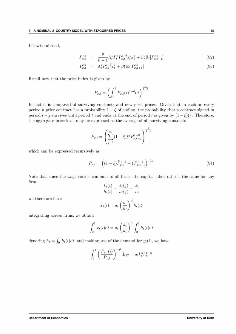
Recall now that the price index is given by

Pt =

(∫ 1

0Pt(i)

1−θdi

) 11−θ

In fact it is composed of surviving contracts and newly set prices. Given that in each an everyperiod a price contract has a probability 1− ξ of ending, the probability that a contract signed in



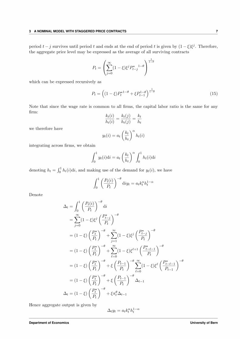
period t− j survives until period t and ends at the end of period t is given by (1− ξ)ξj . Therefore,the aggregate price level may be expressed as the average of all surviving contracts

Pt =

∞∑j=0

(1− ξ)ξjP ?t−j1−θ

11−θ

which can be expressed recursively as

Pt =(

(1− ξ)P ?t1−θ + ξP 1−θ

t−1

) 11−θ

(15)

Note that since the wage rate is common to all firms, the capital labor ratio is the same for anyfirm:

kt(i)

ht(i)=kt(j)

ht(j)=ktht

we therefore have

yt(i) = at

(ktht

)αht(i)

integrating across firms, we obtain∫ 1

0yt(i)di = at

(ktht

)α ∫ 1

0ht(i)di

denoting ht =∫ 1

0 ht(i)di, and making use of the demand for yt(i), we have∫ 1

0

(Pt(i)

Pt

)−θdiyt = atk

αt h

1−αt

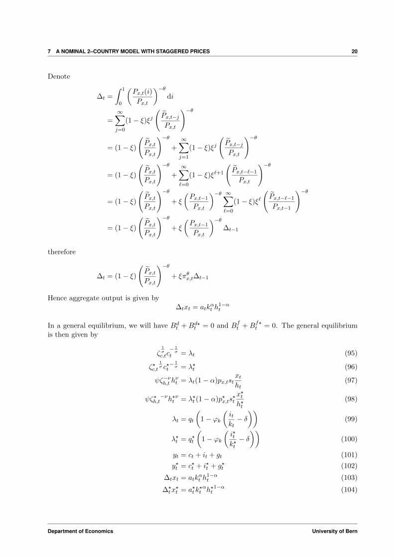
Denote

∆t =

∫ 1

0

(Pt(i)

Pt

)−θdi

=

∞∑j=0

(1− ξ)ξj(P ?t−jPt

)−θ

= (1− ξ)(P ?tPt

)−θ+

∞∑j=1

(1− ξ)ξj(P ?t−jPt

)−θ

= (1− ξ)(P ?tPt

)−θ+

∞∑`=0

(1− ξ)ξ`+1

(P ?t−`−1

Pt

)−θ= (1− ξ)

(P ?tPt

)−θ+ ξ

(Pt−1

Pt

)−θ ∞∑`=0

(1− ξ)ξ`(P ?t−`−1

Pt−1

)−θ= (1− ξ)

(P ?tPt

)−θ+ ξ

(Pt−1

Pt

)−θ∆t−1

∆t = (1− ξ)(P ?tPt

)−θ+ ξπθt∆t−1

Hence aggregate output is given by∆tyt = atk

αt h

1−αt



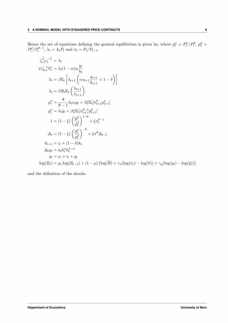
Hence the set of equations defining the general equilibrium is given by, where pnt = Pnt /Pθt , pdt =

P dt /Pθ−1t , λt = ΛtPt and πt = Pt/Pt−1.

ζ1σc,tc− 1σ

t = λt


ytht

λt = βEt[λt+1

(αst+1

yt+1

kt+1+ 1− δ

)]λt = βRtEt

(λt+1

πt+1

)pnt =

θ

θ − 1λtstyt + βξEt[πθt+1p

nt+1]

pdt = λtyt + βξEt[πθ−1t+1 p

dt+1]

1 = (1− ξ)(pntpdt

)1−θ+ ξπθ−1

t

∆t = (1− ξ)(pntpdt

)−θ+ ξπθ∆t−1

kt+1 = it + (1− δ)kt∆tyt = atk

αt h

1−αt

yt = ct + it + gt


)and the definition of the shocks.


4 A SMALL OPEN ECONOMY MODEL WITH STAGGERED PRICES 9

4 A Small Open Economy Model with Staggered Prices

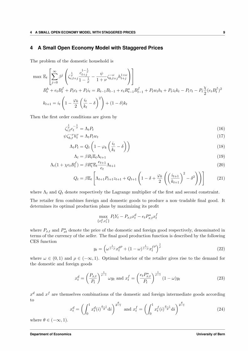
The problem of the domestic household is

max Et

∞∑j=0

βj

ζ 1σc,t+j

c1− 1

σt+j

1− 1σ

− ψ

1 + νζ−νh,t+jh

1+νt+j

Bht + etB

ft + Ptct + Ptit = Rt−1Bt−1 + etR

?t−1B

ft−1 + Ptwtht + Ptztkt − Ptτt − Pt

χ

2(etB

ft )2

kt+1 = it

(1− ϕk

2

(itkt− δ)2)

+ (1− δ)kt


ζ1σc,tc− 1σ

t = ΛtPt (16)


ΛtPt = Qt

(1− ϕk

(itkt− δ))

(18)


Λt(1 + χetBft ) = βR?tEt

et+1

etΛt+1 (20)

Qt = βEt

[Λt+1Pt+1zt+1 +Qt+1

(1− δ +

ϕk2

((it+1

kt+1

)2

− δ2

))](21)

where Λt and Qt denote respectively the Lagrange multiplier of the first and second constraint.

The retailer firm combines foreign and domestic goods to produce a non–tradable final good. Itdetermines its optimal production plans by maximizing its profit

max{xdt ,x

ft }PtYt − Px,txdt − etP ?x,tx

ft

where Px,t and P ?xt denote the price of the domestic and foreign good respectively, denominated interms of the currency of the seller. The final good production function is described by the followingCES function

yt =(ω

11−ρxdt

ρ+ (1− ω)

11−ρxft

ρ) 1ρ

(22)

where ω ∈ (0, 1) and ρ ∈ (−∞, 1). Optimal behavior of the retailer gives rise to the demand forthe domestic and foreign goods

xdt =

(Px,tPt

) 1ρ−1

ωyt and xft =

(etP

?x,t

Pt

) 1ρ−1

(1− ω)yt (23)

xd and xf are themselves combinations of the domestic and foreign intermediate goods accordingto

xdt =

(∫ 1

0xdt (i)

θ−1θ di

) θθ−1

and xft =

(∫ 1

0xft (i)

θ−1θ di

) θθ−1

(24)

where θ ∈ (−∞, 1).



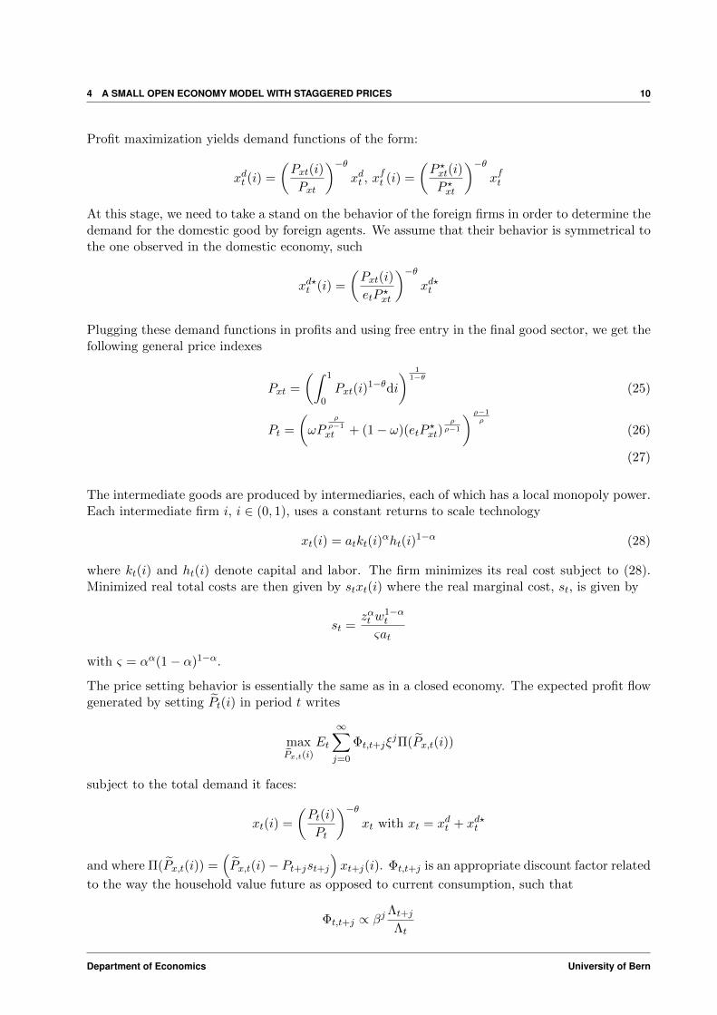
Profit maximization yields demand functions of the form:

xdt (i) =

(Pxt(i)

Pxt

)−θxdt , x

ft (i) =

(P ?xt(i)

P ?xt

)−θxft

At this stage, we need to take a stand on the behavior of the foreign firms in order to determine thedemand for the domestic good by foreign agents. We assume that their behavior is symmetrical tothe one observed in the domestic economy, such

xd?t (i) =

(Pxt(i)

etP ?xt

)−θxd?t

Plugging these demand functions in profits and using free entry in the final good sector, we get thefollowing general price indexes

Pxt =

(∫ 1

0Pxt(i)

1−θdi

) 11−θ

(25)

Pt =

(ωP

ρρ−1

xt + (1− ω)(etP?xt)

ρρ−1

) ρ−1ρ

(26)

(27)

The intermediate goods are produced by intermediaries, each of which has a local monopoly power.Each intermediate firm i, i ∈ (0, 1), uses a constant returns to scale technology

xt(i) = atkt(i)αht(i)

1−α (28)


st =zαt w

1−αt

ςat


The price setting behavior is essentially the same as in a closed economy. The expected profit flowgenerated by setting P̃t(i) in period t writes

maxP̃x,t(i)

Et

∞∑j=0

Φt,t+jξjΠ(P̃x,t(i))


xt(i) =

(Pt(i)

Pt

)−θxt with xt = xdt + xd?t

and where Π(P̃x,t(i)) =(P̃x,t(i)− Pt+jst+j

)xt+j(i). Φt,t+j is an appropriate discount factor related

to the way the household value future as opposed to current consumption, such that





Et

∞∑j=0

(βξ)jΛt+jΛt

(1− θ)

(P̃x,t(i)

Px,t+j

)−θyt+j + θ

Pt+jPx,t+j(i)

(P̃x,t(i)

Px,t+j

)−θst+jxt+j

= 0

from which it shall be clear that all firms that reset their price in period t set it at the same level(P̃t(i) = P̃t, for all i ∈ (0, 1)). This implies that

P̃x,t =P nx,t

P dx,t

(29)

where

Pnx,t = Et

∞∑j=0

(βξ)jΛt+jθ

θ − 1Pt+jP

θx,t+jst+jxt+j

and

P dx,t = Et

∞∑j=0

(βξ)jΛt+jPθx,t+jxt+j


x,t and P dx,t admit a recursive representation, such that

Pnx,t =θ

θ − 1ΛtPtP

θx,tstxt + βξEt[Pnx,t+1] (30)

P dx,t = ΛtPθx,txt + βξEt[P dx,t+1] (31)


Px,t =

(∫ 1

0Px,t(i)

1−θdi

) 11−θ

In fact it is composed of surviving contracts and newly set prices. Given that in each an everyperiod a price contract has a probability 1− ξ of ending, the probability that a contract signed inperiod t− j survives until period t and ends at the end of period t is given by (1− ξ)ξj . Therefore,the aggregate price level may be expressed as the average of all surviving contracts

Px,t =

∞∑j=0

(1− ξ)ξjP̃ 1−θx,t−j

11−θ


Px,t =(

(1− ξ)P̃ 1−θx,t + ξP 1−θ

x,t−1

) 11−θ

(32)


kt(i)

ht(i)=kt(j)

ht(j)=ktht

we therefore have

xt(i) = at

(ktht

)αht(i)




0xt(i)di = at

(ktht

)α ∫ 1

0ht(i)di

denoting ht =∫ 1


0

(Px,t(i)

Px,t

)−θdiyt = atk

αt h

1−αt

Denote

∆t =

∫ 1

0

(Px,t(i)

Px,t

)−θdi

=∞∑j=0

(1− ξ)ξj(P̃x,t−jPx,t

)−θ

= (1− ξ)

(P̃x,tPx,t

)−θ+∞∑j=1


)−θ

= (1− ξ)

(P̃x,tPx,t

)−θ+∞∑`=0

(1− ξ)ξ`+1

(P̃x,t−`−1

Px,t

)−θ

= (1− ξ)

(P̃x,tPx,t

)−θ+ ξ

(Px,t−1

Px,t

)−θ ∞∑`=0

(1− ξ)ξ`(P̃x,t−`−1

Px,t−1

)−θ

= (1− ξ)

(P̃x,tPx,t

)−θ+ ξ

(Px,t−1

Px,t

)−θ∆t−1

∆t = (1− ξ)

(P̃x,tPx,t

)−θ+ ξπθx,t∆t−1

Hence aggregate output is given by∆txt = atk

αt h

1−αt

The behavior of the foreign economy is assumed to be very similar to the one observed domestically.We however assumethat foreign output and prices are exogenously given and modelled as AR(1)processes. We further assume that P ?x,t = P ?t . The foreign household’s saving behavior is the sameas in the domestic economy (absent preference shocks), such that the foreign nomina interest rateis given by

y?t− 1σ = βR?tEty?t+1

− 1σP ?tP ?t+1

We assume that foreign households do not buy domestic bonds, which implies that in equilibriumBdt = 0.



The general equilibrium is then given by

ζ1σc,tc− 1σ

t = λt (33)


px,txtht

(34)

λt = qt

(1− ϕk

(itkt− δ))

(35)

yt = ct + it + gt +χ

2bf2t (36)

∆txt = atkαt h

1−αt (37)

xdt = p1ρ−1

x,t ωyt (38)

xd?t =

(px,trert

) 1ρ−1

(1− ω)y?t (39)

xft = (rertp?x,t)

1ρ−1 (1− ω)yt (40)

xt = xdt + xd?t (41)

1 = ωpρρ−1

x,t + (1− ω)(rertp?t )

ρρ−1 (42)

λt = βRtEtλt+1

πt+1(43)

λt(1 + χbft ) = βR?tEt∆et+1

πt+1λt+1 (44)

qt = βEt

[λt+1αst+1

px,t+1xt+1

kt+1+ qt+1

(1− δ +

ϕk2

((it+1

kt+1

)2

− δ2

))](45)

bft =∆et

πtR?t−1b

ft−1 + px,txt − yt (46)

kt+1 = it

(1− ϕk

2

(itkt− δ)2)

+ (1− δ)kt (47)

rert =∆etp?t

πtp?t−1

rert−1 (48)

px,t =πx,tπt

px,t−1 (49)


)(50)

pnx,t =θ

θ − 1λtp

θx,tstxt + βξEt[pnx,t+1π

θt+1] (51)

pdx,t = λtpθx,txt + βξEt[pdx,t+1π

θ−1t+1 ] (52)

px,t =

(1− ξ)

(pnx,t

pdx,t

)1−θ

+ ξ

(px,t−1

πt

)1−θ 1

1−θ

(53)

∆t = (1− ξ)

(pnx,t

px,tpdx,t

)−θ+ ξ∆t−1π

θx,t (54)

y?t− 1σ = βR?Ety?t+1

− 1σp?tp?t+1

(55)

where λt = ΛtPt, rert = etP?t /Pt, px,t = Px,t/Pt, p

nt = Pnt /P

θt , pdt = P dt /P

θ−1t , πt = Pt/Pt−1,


6 A REAL SMALL OPEN ECONOMY MODEL 14

πx,t = Px,t/Px,t−1, ∆et = et/et−1.






log(y?t+1) = ρy log(y?t ) + (1− ρy) log(y) + ε?y,t+1

log(p?t+1) = ρp log(p?t ) + (1− ρp) log(p) + ε?p,t+1

5 A Nominal Small Open Economy Model with Price Adjustment Costs

When price contracts are replaced with price adjustment costs, equations (36)–(37) become


2bf2t +

ϕp2

(πx,t − 1)2yt

xt = atkαt h

1−αt

and equations (51)–(54) are replaced with

(1− θ)px,txt + θstxt − ϕpπx,t(πx,t − 1)yt + βEt[λt+1

λtπx,t+1ϕp(πx,t+1 − 1)yt+1

]= 0

6 A Real Small Open Economy Model

All nominal aspects disappear, such that the general equilibrium becomes

ζ1σc,tc− 1σ

t = λt (56)

ψζ−νh,t hνt = λt(1− α)

px,txtht

(57)

λt = qt

(1− ϕk

(itkt− δ))

(58)


2bf2t (59)

xt = atkαt h

1−αt (60)

xdt = p1ρ−1

x,t ωyt (61)

xd?t =

(px,trert

) 1ρ−1

(1− ω)y?t (62)

xft = (rertp?x,t)

1ρ−1 (1− ω)yt (63)

xt = xdt + xd?t (64)

1 = ωpρρ−1

x,t + (1− ω)(rertp?t )

ρρ−1 (65)


6 A REAL SMALL OPEN ECONOMY MODEL 15

λt = βRtEtλt+1 (66)

λt(1 + χbft ) = βR?tEtλt+1 (67)

qt = βEt

[λt+1α

px,t+1xt+1

kt+1+ qt+1

(1− δ +

ϕk2

((it+1

kt+1

)2

− δ2

))](68)

bft = R?t−1bft−1 + px,txt − yt (69)

kt+1 = it

(1− ϕk

2

(itkt− δ)2)

+ (1− δ)kt (70)

y?t− 1σ = βR?tEty?t+1

− 1σ (71)

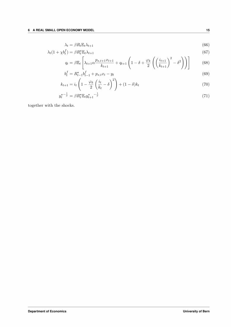
together with the shocks.


7 A NOMINAL 2–COUNTRY MODEL WITH STAGGERED PRICES 16

7 A Nominal 2–Country Model with Staggered Prices

The problem of the domestic household is

max Et

∞∑j=0

βj

ζ 1σc,t+j

c1− 1

σt+j

1− 1σ

− ψ

1 + νζ−νh,t+jh

1+νt+j

Bht + etB

ft + Ptct + Ptit = Rt−1Bt−1 + etR

?t−1B

ft−1 + Ptwtht + Ptztkt − Ptτt

kt+1 = it

(1− ϕk

2

(itkt− δ)2)

+ (1− δ)kt


ζ1σc,tc− 1σ

t = ΛtPt (72)


ΛtPt = Qt

(1− ϕk

(itkt− δ))

(74)


Λt = βR?tEtet+1

etΛt+1 (76)

Qt = βEt

[Λt+1Pt+1zt+1 +Qt+1

(1− δ +

ϕk2

((it+1

kt+1

)2

− δ2

))](77)

where Λt and Qt denote respectively the Lagrange multiplier of the first and second constraint.The behavior of the foreign household, hereafter denoted by a ?, is totally symmetrical. We furtherhave the following risk sharing condition

Λt =Λ?tet

The retailer firm combines foreign and domestic goods to produce a non–tradable final good. Itdetermines its optimal production plans by maximizing its profit

max{xdt ,x

ft }PtYt − Px,txdt − etP ?x,tx

ft

where Px,t and P ?xt denote the price of the domestic and foreign good respectively, denominated interms of the currency of the seller. The final good production function is described by the followingCES function

yt =(ω

11−ρxdt

ρ+ (1− ω)

11−ρxft

ρ) 1ρ

(78)

where ω ∈ (0, 1) and ρ ∈ (−∞, 1). Optimal behavior of the retailer gives rise to the demand forthe domestic and foreign goods

xdt =

(Px,tPt

) 1ρ−1

ωyt and xft =

(etP

?x,t

Pt

) 1ρ−1

(1− ω)yt (79)

Abroad, the behavior is symmetrical, such that

y?t =(ω

11−ρxf?t

ρ+ (1− ω)

11−ρxd?t

ρ) 1ρ

(80)



and

xd?t =

(Px,tetP ?t

) 1ρ−1

(1− ω)y?t and xf?t =

(P ?x,tP ?t

) 1ρ−1

ωy?t (81)

xd and xf are themselves combinations of the domestic and foreign intermediate goods accordingto

xdt =

(∫ 1

0xdt (i)

θ−1θ di

) θθ−1

and xft =

(∫ 1

0xft (i)

θ−1θ di

) θθ−1

(82)

where θ ∈ (−∞, 1). Likewise abroad

xd?t =

(∫ 1

0xd?t (i)

θ−1θ di

) θθ−1

and xf?t =

(∫ 1

0xf?t (i)

θ−1θ di

) θθ−1

(83)

Profit maximization yields demand functions of the form:

xdt (i) =

(Pxt(i)

Pxt

)−θxdt , x

ft (i) =

(P ?xt(i)

P ?xt

)−θxft ,

similarly abroad

xd?t (i) =

(Pxt(i)

Pxt

)−θxd?t , x

f?t (i) =

(P ?xt(i)

P ?xt

)−θxf?t

Plugging these demand functions in profits and using free entry in the final good sector, we get thefollowing general price indexes

Pxt =

(∫ 1

0Pxt(i)

1−θdi

) 11−θ

, P ?xt =

(∫ 1

0P ?xt(i)

1−θdi

) 11−θ

(84)

Pt =

(ωP

ρρ−1

xt + (1− ω)(etP?xt)

ρρ−1

) ρ−1ρ

(85)

P ?t =

(ω

(Pxtet

) ρρ−1

+ (1− ω)P ?xtρρ−1

) ρ−1ρ

(86)

The intermediate goods are produced by intermediaries, each of which has a local monopoly power.Each intermediate firm i, i ∈ (0, 1), uses a constant returns to scale technology

xt(i) = atkt(i)αht(i)

1−α (87)


st =zαt w

1−αt

ςat

with ς = αα(1− α)1−α. Similarly abroad

x?t (i) = a?tk?t (i)

αh?t (i)1−α (88)



where k?t (i) and h?t (i) denote capital and labor. The firm minimizes its real cost subject to (87).Minimized real total costs are then given by s?tx

?t (i) where the real marginal cost, s?t , is given by

s?t =z?tαw?t

1−α

ςa?t


The price setting behavior is essentially the same as in a closed economy. The expected profit flowgenerated by setting P̃t(i) in period t writes

maxP̃x,t(i)

Et

∞∑j=0

Φt,t+jξjΠ(P̃x,t(i))


xt(i) =

(Pt(i)

Pt

)−θxt with xt = xdt + xd?t

and where Π(P̃x,t(i)) =(P̃x,t(i)− Pt+jst+j

)xt+j(i). Φt,t+j is an appropriate discount factor related

to the way the household value future as opposed to current consumption, such that



Et

∞∑j=0

(βξ)jΛt+jΛt

(1− θ)

(P̃x,t(i)

Px,t+j

)−θyt+j + θ

Pt+jPx,t+j(i)

(P̃x,t(i)

Px,t+j

)−θst+jxt+j

= 0

from which it shall be clear that all firms that reset their price in period t set it at the same level(P̃t(i) = P̃t, for all i ∈ (0, 1)). This implies that

P̃x,t =P nx,t

P dx,t

(89)

where

Pnx,t = Et

∞∑j=0

(βξ)jΛt+jθ

θ − 1Pt+jP

θx,t+jst+jxt+j

and

P dx,t = Et

∞∑j=0

(βξ)jΛt+jPθx,t+jxt+j


x,t and P dx,t admit a recursive representation, such that

Pnx,t =θ

θ − 1ΛtPtP

θx,tstxt + βξEt[Pnx,t+1] (90)

P dx,t = ΛtPθx,txt + βξEt[P dx,t+1] (91)



Likewise abroad,

Pn?x,t =θ

θ − 1Λ?tP

?t P

?x,tθs?tx

?t + βξEt[Pn?x,t+1] (92)

P d?x,t = Λ?tP?x,tθx?t + βξEt[P d?x,t+1] (93)


Px,t =

(∫ 1

0Px,t(i)

1−θdi

) 11−θ

In fact it is composed of surviving contracts and newly set prices. Given that in each an everyperiod a price contract has a probability 1− ξ of ending, the probability that a contract signed inperiod t− j survives until period t and ends at the end of period t is given by (1− ξ)ξj . Therefore,the aggregate price level may be expressed as the average of all surviving contracts

Px,t =

∞∑j=0

(1− ξ)ξjP̃ 1−θx,t−j

11−θ


Px,t =(

(1− ξ)P̃ 1−θx,t + ξP 1−θ

x,t−1

) 11−θ

(94)


kt(i)

ht(i)=kt(j)

ht(j)=ktht

we therefore have

xt(i) = at

(ktht

)αht(i)


0xt(i)di = at

(ktht

)α ∫ 1

0ht(i)di

denoting ht =∫ 1


0

(Px,t(i)

Px,t

)−θdiyt = atk

αt h

1−αt



Denote

∆t =

∫ 1

0

(Px,t(i)

Px,t

)−θdi

=

∞∑j=0


)−θ

= (1− ξ)

(P̃x,tPx,t

)−θ+

∞∑j=1


)−θ

= (1− ξ)

(P̃x,tPx,t

)−θ+∞∑`=0

(1− ξ)ξ`+1

(P̃x,t−`−1

Px,t

)−θ

= (1− ξ)

(P̃x,tPx,t

)−θ+ ξ

(Px,t−1

Px,t

)−θ ∞∑`=0

(1− ξ)ξ`(P̃x,t−`−1

Px,t−1

)−θ

= (1− ξ)

(P̃x,tPx,t

)−θ+ ξ

(Px,t−1

Px,t

)−θ∆t−1

therefore

∆t = (1− ξ)

(P̃x,tPx,t

)−θ+ ξπθx,t∆t−1

Hence aggregate output is given by∆txt = atk

αt h

1−αt

In a general equilibrium, we will have Bdt + Bd?

t = 0 and Bft + Bf?

t = 0. The general equilibriumis then given by

ζ1σc,tc− 1σ

t = λt (95)

ζ?c,t1σ c?t− 1σ = λ?t (96)

ψζ−νh,t hνt = λt(1− α)px,tst

xtht

(97)

ψζ?h,t−νh?t

ν = λ?t (1− α)p?x,ts?t

x?th?t

(98)

λt = qt

(1− ϕk

(itkt− δ))

(99)

λ?t = q?t

(1− ϕk

(i?tk?t− δ))

(100)

yt = ct + it + gt (101)

y?t = c?t + i?t + g?t (102)

∆txt = atkαt h

1−αt (103)

∆?tx?t = a?tk

?tαh?t

1−α (104)



xdt = p1ρ−1

x,t ωyt (105)

xd?t =

(px,trert

) 1ρ−1

(1− ω)y?t (106)

xft = (rertp?x,t)

1ρ−1 (1− ω)yt (107)

xf?t = p?x,t1ρ−1ωy?t (108)

xt = xdt + xd?t (109)

x?t = xft + xf?t (110)

1 = ωpρρ−1

x,t + (1− ω)(rertp?x,t)

ρρ−1 (111)

1 = ωp?x,tρρ−1 + (1− ω)

(p?x,trert

) ρρ−1

(112)

λt =λ?trert

(113)

λt = βRtEtλt+1

πt+1(114)

qt = βEt

[λt+1αst+1

px,t+1xt+1

kt+1+ qt+1

(1− δ +

ϕk2

((it+1

kt+1

)2

− δ2

))](115)

q?t = βEt

[λ?t+1αs

?t+1

p?x,t+1x?t+1

k?t+1

+ q?t+1

(1− δ +

ϕk2

((i?t+1

k?t+1

)2

− δ2

))](116)

kt+1 = it

(1− ϕk

2

(itkt− δ)2)

+ (1− δ)kt (117)

k?t+1 = i?t

(1− ϕk

2

(i?tk?t− δ)2)

+ (1− δ)k?t (118)

Rt = R?tEt∆et+1 (119)

rert =∆etπ?t

πtrert−1 (120)

px,t =πx,tπt

px,t−1 (121)

p?x,t =π?x,tπ?t

p?x,t−1 (122)


)(123)

log(R?t ) = ρr log(R?t−1) + (1− ρ)(log(R) + γπ(log(π?t )− log(π)) + γy(log(y?t )− log(y))

)(124)

pnx,t =θ

θ − 1λtp

θx,tstxt + βξEt[pnx,t+1π

θt+1] (125)

pn?x,t =θ

θ − 1λ?t p

?x,tθs?tx

?t + βξEt[pn?x,t+1π

?θt+1] (126)

pdx,t = λtpθx,txt + βξEt[pdx,t+1π

θ−1t+1 ] (127)

pd?x,t = λ?t p?x,tθx?t + βξEt[pd?x,t+1π

?θ−1x,t+1] (128)


8 A NOMINAL 2–COUNTRY MODEL WITH PRICE ADJUSTMENT COSTS 22

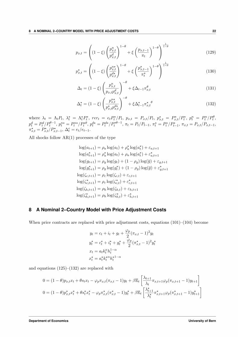
px,t =

(1− ξ)

(pnx,t

pdx,t

)1−θ

+ ξ

(px,t−1

πt

)1−θ 1

1−θ

(129)

p?x,t =

(1− ξ)

(pn?x,t

pd?x,t

)1−θ

+ ξ

(p?x,t−1

π?t

)1−θ 1

1−θ

(130)

∆t = (1− ξ)

(pnx,t

px,tpdx,t

)−θ+ ξ∆t−1π

θx,t (131)

∆?t = (1− ξ)

(pn?x,t

p?x,tpd?x,t

)−θ+ ξ∆?

t−1π?x,tθ (132)

where λt = ΛtPt, λ?t = Λ?tP

?t , rert = etP

?t /Pt, px,t = Px,t/Pt, p

?x,t = P ?x,t/P

?t , pnt = Pnt /P

θt ,

pdt = P dt /Pθ−1t , pn?t = Pn?t /P ?θt , pd?t = P d?t /P ?θ−1

t , πt = Pt/Pt−1, π?t = P ?t /P?t−1, πx,t = Px,t/Px,t−1,

π?x,t = P ?x,t/P?x,t−1, ∆e

t = et/et−1.


log(at+1) = ρa log(at) + ρ?a log(a?t ) + εa,t+1

log(a?t+1) = ρ?a log(at) + ρa log(a?t ) + ε?a,t+1


log(g?t+1) = ρg log(g?t ) + (1− ρg) log(g) + ε?g,t+1


log(ζ?c,t+1) = ρc log(ζ?c,t) + ε?c,t+1


log(ζ?h,t+1) = ρh log(ζ?h,t) + ε?h,t+1

8 A Nominal 2–Country Model with Price Adjustment Costs

When price contracts are replaced with price adjustment costs, equations (101)–(104) become

yt = ct + it + gt +ϕp2

(πx,t − 1)2yt

y?t = c?t + i?t + g?t +ϕp2

(π?x,t − 1)2y?t

xt = atkαt h

1−αt

x?t = a?tk?tαh?t

1−α

and equations (125)–(132) are replaced with

0 = (1− θ)px,txt + θstxt − ϕpπx,t(πx,t − 1)yt + βEt[λt+1

λtπx,t+1ϕp(πx,t+1 − 1)yt+1

]0 = (1− θ)p?x,tx?t + θs?tx

?t − ϕpπ?x,t(π?x,t − 1)y?t + βEt

[λ?t+1

λ?tπ?x,t+1ϕp(π

?x,t+1 − 1)y?t+1

]


9 A REAL 2–COUNTRY MODEL 23

9 A Real 2–Country Model

All nominal aspects disappear, such that the general equilibrium becomes

ζ1σc,tc− 1σ

t = λt (133)

ζ?c,t1σ c?t− 1σ = λ?t (134)

ψζ−νh,t hνt = λt(1− α)px,t

xtht

(135)

ψζ?h,t−νh?t

ν = λ?t (1− α)p?x,tx?th?t

(136)

λt = qt

(1− ϕk

(itkt− δ))

(137)

λ?t = q?t

(1− ϕk

(i?tk?t− δ))

(138)

yt = ct + it + gt (139)

y?t = c?t + i?t + g?t (140)

xdt = p1ρ−1

x,t ωyt (141)

xd?t =

(px,trert

) 1ρ−1

(1− ω)y?t (142)

xft = (rertp?x,t)

1ρ−1 (1− ω)yt (143)

xf?t = p?x,t1ρ−1ωy?t (144)

xt = xdt + xd?t (145)

x?t = xft + xf?t (146)

xt = atkαt h

1−αt (147)

x?t = a?tk?tαh?t

1−α (148)

1 = ωpρρ−1

x,t + (1− ω)(rertp?x,t)

ρρ−1 (149)

1 = ωp?x,tρρ−1 + (1− ω)

(p?x,trert

) ρρ−1

(150)

λt = λ?t (151)

qt = βEt

[λt+1α

px,t+1xt+1

kt+1+ qt+1

(1− δ +

ϕk2

((it+1

kt+1

)2

− δ2

))](152)

q?t = βEt

[λ?t+1α

p?x,t+1x?t+1

k?t+1

+ q?t+1

(1− δ +

ϕk2

((i?t+1

k?t+1

)2

− δ2

))](153)

kt+1 = it

(1− ϕk

2

(itkt− δ)2)

+ (1− δ)kt (154)

k?t+1 = i?t

(1− ϕk

2

(i?tk?t− δ)2)

+ (1− δ)k?t (155)


A Suite of Models for Dynare - fabcol.free.frfabcol.free.fr/dynare/pdf/models.pdf · A Suite of...

Documents

Transcript of A Suite of Models for Dynare - fabcol.free.frfabcol.free.fr/dynare/pdf/models.pdf · A Suite of...