arX

iv:1

401.

2395

v2 [

stat

.CO

] 3

1 Ju

l 201

4

The Annals of Applied Statistics

2014, Vol. 8, No. 2, 1119–1144DOI: 10.1214/14-AOAS716c© Institute of Mathematical Statistics, 2014

A STATISTICAL APPROACH TO THE INVERSE PROBLEMIN MAGNETOENCEPHALOGRAPHY

By Zhigang Yao1,∗ and William F. Eddy†

Ecole Polytechnique Federale de Lausanne∗ and Carnegie MellonUniversity†

Magnetoencephalography (MEG) is an imaging technique used tomeasure the magnetic field outside the human head produced by theelectrical activity inside the brain. The MEG inverse problem, iden-tifying the location of the electrical sources from the magnetic signalmeasurements, is ill-posed, that is, there are an infinite number ofmathematically correct solutions. Common source localization meth-ods assume the source does not vary with time and do not provideestimates of the variability of the fitted model. Here, we reformulatethe MEG inverse problem by considering time-varying locations forthe sources and their electrical moments and we model their timeevolution using a state space model. Based on our predictive model,we investigate the inverse problem by finding the posterior sourcedistribution given the multiple channels of observations at each timerather than fitting fixed source parameters. Our new model is morerealistic than common models and allows us to estimate the variationof the strength, orientation and position. We propose two new MonteCarlo methods based on sequential importance sampling. Unlike theusual MCMC sampling scheme, our new methods work in this situ-ation without needing to tune a high-dimensional transition kernelwhich has a very high cost. The dimensionality of the unknown pa-rameters is extremely large and the size of the data is even larger. Weuse Parallel Virtual Machine (PVM) to speed up the computation.

1. Introduction.

1.1. The basics of magnetoencephalography (MEG). The anatomy of thebrain has been studied intensively for millennia, yet how the brain functionsis still not well understood. The neurons in the brain produce macroscopicelectrical currents when the brain functions, and those synchronized neu-

Received January 2012; revised January 2014.1Supported in part by NSF SES-1061387 and NIH/NIDA R90 DA023420.Key words and phrases. Ill-posed problem, sequential importance sampling, state space

model, parallel computing, source localization.

This is an electronic reprint of the original article published by theInstitute of Mathematical Statistics in The Annals of Applied Statistics,2014, Vol. 8, No. 2, 1119–1144. This reprint differs from the original in paginationand typographic detail.

1

2 Z. YAO AND W. F. EDDY

ronal currents in the gray matter of the brain induce extremely weak mag-netic fields (10–100 femto-Tesla) outside the head. The comparatively recentdevelopment of the Superconducting Quantum Interference Device (SQUID)makes it possible to detect those magnetic signals. MEG is an imaging tech-nique using SQUIDs to measure the magnetic signals outside of the headproduced by the electrical activity inside the brain [Cohen (1968)]. Theprimary sources are electric currents within the dendrites of the large pyra-midal cells of activated neurons in the human cortex, generally formulatedas a mathematical point current dipole. Such focal brain activation can beobserved in epilepsy, or it can be induced by a stimulus in neurophysiologicalor neuropsychological experiments. Due to its noninvasiveness (it is a com-pletely passive measurement method) and its impressive temporal resolution(better than 1 millisecond, compared to 1 second for functional magnetic res-onance imaging, or to 1 minute for positron emission tomography), and dueto the fact that the signal it measures is a direct consequence of neural activ-ity, MEG is a near optimal tool for studying brain activity, such as assistingsurgeons in localizing a pathology, assisting researchers in determining brainfunction, neuro-feedback and others. The skull and the tissue surroundingthe brain affect the magnetic fields measured by MEG much less than theelectrical impulses measured by electroencephalography (EEG). This meansthat MEG has higher localization accuracy than the EEG and it allows for amore reliable localization of brain function [Hamalainen et al. (1993), Okada,Lahteenmaki and Xu (1999)]. MEG has recently been used in the evaluationof epilepsy, where it reveals the exact location of the abnormalities, whichmay then allow physicians to find the cause of the seizures [Barkley andBaumgartner (2003)]. MEG is also reference free, so that the localization ofsources with a given precision is easier for MEG than it is for EEG [Kristeva-Feige et al. (1997)]. The computation associated with estimating the electricsource from the magnetic measurement is a challenging problem that needsto be solved to allow high temporal and spatial resolution imaging of thedynamic activity of the human brain.

1.2. Forward and inverse MEG problem. The MEG signals derive fromthe primary current (the net effect of ionic currents flowing in the dendritesof neurons) and the volume current (i.e., the additive ohmic current set up inthe surrounding medium to complete the electrical circuit). If the electricalsource is known and the head model [Kybic et al. (2006)] is specified (e.g.,a sphere with homogeneous conductivity), then the “forward problem” is tocompute the electric field E and the magnetic field B from the source currentJ. The calculation uses Maxwell’s equations [see, e.g., Griffiths (1999)],

∇ ·E= ρ/ε0,

∇×E=−∂B/∂t,

MEG INVERSE PROBLEM 3

∇ ·B= 0,

∇×B= µ0(J+ ε0 ∂E/∂t),

where ε0 and µ0 are the permittivity and permeability of a vacuum, re-spectively, and ρ is the charge density. The total current J consists of theprimary current JP plus the volume current JV. The source activity in thebrain corresponds to the primary current. Under reasonable assumptions[see Hamalainen et al. (1993)], the volume current JV is not included inthe analysis because of its diffuse nature. The terms ∂B/∂t and ∂E/∂t inMaxwell’s equations can be ignored by assuming that the magnetic fieldvaries relatively slowly in time. Rather than working with continuous elec-tric current, the most frequently used computational model assumes that theelectric current can be thought of as an electric dipole; this model is calledan equivalent current dipole (ECD); see, for example, Hamalainen et al.(1993). From the perspective of an ECD, a dipole has location, orientationand magnitude; the magnetic field generated by this dipole can explain theMEG measurements. In addition, there is a version of an ECD model as-suming multiple dipoles; from Maxwell’s equations it is easy to see that thismodel is simply the sum of the models for each ECD. Such an ECD modelsa large number of dipoles located at fixed places over the cortical surface. Inneuroscience, it is believed that typical MEG data should be explained byonly a few dipoles (less than 10), and different criteria or algorithms are usedto minimize the number of dipoles in various ECD models; we discuss someof these models in Section 1.3. We assume that E is generated by JP, whichin turn comes from the sum of N localized current dipoles at locations rn,

JPn(r) =Qnδ(r− rn), n= 1, . . . ,N,

where δ(·) is the Dirac delta function. The Qn is a charged dipole at thepoint rn in the brain volume Ω. Using the quasi-static approximation toMaxwell’s equations (i.e., ignoring the partial derivatives with respect totime) given in Sarvas (1984), the magnetic field B at location r of a currentdipole at rn can be calculated by the Biot–Savart equation,

Bn(r) =µ0

4π

∫

Ω

JP(rn)× (r− rn)

|r− rn|3drn.

In the case of multiple current dipoles, the induced magnetic fields simplyadd up.

The “inverse problem” comes from the forward model; we want to es-timate the dipole parameters from the observed magnetic signal. The diffi-culty is that there is not a unique solution; there are infinitely many differentsources within the skull that produce the same observed data. The goal isto find a meaningful solution among the many mathematically correct so-lutions. There are three key steps to any source localization algorithm in

4 Z. YAO AND W. F. EDDY

MEG. First, define the solution space and the parameter space of the elec-tric source. Second, calculate the magnetic field given the information aboutthe head model. Third, according to what criterion the solution must satisfy,perform an extensive search for the solution. Methods of finding the sourcefrom the observed MEG signal have been extensively exploited during thepast two decades, mostly centered on finding a single estimate of the source.Some of these methods are briefly described in the next subsection. However,finding the distribution of the source in space and (particularly) in time isstill a problem requiring investigation.

1.3. Existing source localization methods. Most methods for localizingelectrical sources in MEG assume that the electrical sources in the braindo not include a temporal component. The data are used to estimate thesource parameters at each time point; there is no relation to the estimatesfor the previous time. This is not the same as assuming the quasi-staticapproximation to Maxwell’s equations. Therefore, those existing methodsare restricted to fixed dipole assumptions and are also not able to provideestimates of the variability of source activity. The minimum norm estimate(MNE) [Hamalainen and Ilmoniemi (1994)] is a regularization method basedon the L2 norm. The L1 norm regularization yields the minimum current es-timates (MCE) [Uutela, Hamalainen and Somersalo (1999)]. The LORETAapproach [Mattout et al. (2006)] is a special case of weighted MNE. TheMultiple Signal Classification method (MUSIC) [Mosher, Lewis and Leahy(1992)] searches for a single-dipole model through a three-dimensional headvolume and computes projections onto an estimated signal subspace. Thesource locations are then found as the 3-D locations where the source modelgives the best projections onto the subspace. The beamformer methods[Van Veen, Joseph and Hecox (1992)] ignore the ill-posed inverse problemand instead only estimate the current at several fixed locations. Bayesianapproaches to the MEG inverse problem try to find the posterior distribu-tion of the dipole parameters [Bertrand et al. (2001), Schmidt, George andWood (1999)].

The methods mentioned briefly above (MNE, MCE, etc.) have been widelyused and produce apparently meaningful solutions; however they have overlyrestrictive assumptions and lack estimates of the variability of source esti-mates. By assuming a static localized dipole, these methods are limited intheir ability to incorporate problem-specific anatomical or physiological in-formation. It is quite reasonable to consider that the source is time-varyingrather than fixed, in which case the noise reduction obtained by averagingover consecutive observations in time is problematic. By utilizing a time-varying source model, we will be able to investigate the distribution of thesource at each time point and provide estimates of the variability. Follow-ing this idea, the time evolution of the source is modeled by a state space

MEG INVERSE PROBLEM 5

model. Our goal is to find the posterior distribution of the source parame-ters. Our reformulation of the inverse problem leads to a predictive modelof the dipole. It turns out that the posterior source distribution from ourpredictive model can be interpreted as a statistical solution to the MEGinverse problem.

1.4. Outline of this paper. In Section 2 we develop a time-varying sourcemodel for the MEG inverse problem. Rather than attempting to “solve”the inverse problem we try to develop estimates of the dipole parametersusing a spatio-temporal model. In Section 3 the difficulty of using Markovchain Monte Carlo (MCMC) methods for generating samples from the time-varying model is explained. Then, we introduce the standard SequentialImportance Sampling (SIS) technique. Next, two further Monte Carlo meth-ods are described: (1) the regular SIS method with rejection, and (2) theimproved SIS method with resampling. A simulation study is described inSection 4. We describe our use of the Parallel Virtual Machine (PVM) soft-ware to speed up the computations in Section 4.2. We believe this is the firstapplication of parallel computational methods to the problem. In Section 5a real data application is presented. Section 6 contains a short discussionand conclusion.

2. A probablistic rime-varying source model. Assume that the magneticfield data is measured from the kth sensor at time t as

Yk,t =Bk(JPt ) +Uk,t, 1≤ t≤ T,1≤ k ≤ L,

where Uk,t ∼ N(0, σ21) denotes the observation noise that is assumed, for

simplicity, to be Gaussian, additive and homogeneous for all the sensors,and uncorrelated between every pair of sensors. The assumption of normal-ity is preferred due to the fact that Gaussian sensor noise is present at theMEG sensors themselves, and sensor noise is typically substantially smallerthan signals from spontaneous brain activity [Hamalainen et al. (1993)]. Al-though correlated sensor noise is more realistic than “homogeneous” sensors,it complicates the problem. Background noise and biological noise can alsodrown out the brain activity of interest, but these are all very difficult toincorporate. Besides some variation coming from solving the inverse prob-lem, most of the variation of the source localization in MEG is due to thepropagation of errors through Maxwell’s equations when solving the forwardproblem. In order to control variation, we only work with a simple sensorstructure. Therefore, we write

Yt =B(JPt ) +Ut, 1≤ t≤ T,

whereYt = (Y1,t, . . . , YL,t)T ,B(JP

t ) = (B1(JPt ), . . . ,BL(J

Pt ))

T andUt = (U1,t,. . . ,UL,t)

T . Here, Ut ∼N (0,Σ1), where Σ1 = diag[σ21 , . . . , σ

21].

The Bk(JPt ), a function of the dipole with parameter vector JP

t , is thephysical approximation of the Biot–Savart law in Section 1.2. We consider a

6 Z. YAO AND W. F. EDDY

current dipole located within a horizontally layered conductor [Hamalainenet al. (1993)]. The noiseless magnetic field at the kth sensor, Bk, is computedfrom the source JP

t = (pt,qt) at time t. The vector pt = (p1t, p2t, p3t) con-tains the location parameters of the source and the vector qt = (q1t, q2t, q3t)contains the moments and strength. Thus,

Bk(JPt ) =

µ0

4π

qt × (rk − pt) · e

|rk −pt|3.(1)

Here, rk is the location of the kth sensor. Because the magnetometers mea-sure only the z direction of the magnetic field B, e= (0,0,1), a unit vector,is used to find the z component of B. Conventionally, z is perpendicular tothe surface of the skull.

To specify the prior, the time evolution of the current dipole JPt is modeled

by a state space model. A number of other authors have also proposed statingthe MEG inverse problem as a Bayesian dynamic model; see Somersalo,Voutilainen and Kaipio (2003); Campi et al. (2008, 2011); Sorrentino et al.(2009, 2013); Miao et al. (2013). We could choose any of a large varietyof state space models but, for theoretical and computational simplicity, wehave chosen a six-dimensional first-order autoregression:

JPt =mcom + ρ(JP

t−1 −mcom) +Vt, 1≤ t≤ T,

where Vt ∼N (0,Σ2) denotes the state evolution noise. We note that threeof the parameters give the spatial location, so this is implicitly a space–time model. Previous work using a space–time model [Ou, Hamalainen andGolland (2009)] used a novel mixed L1L2-norm estimate for the dipole pa-rameters based on a linear regression model. Jun et al. (2005) have alsoused MCMC methods for sampling from the posterior of a spatiotemporalBayesian dynamic model. To reduce the number of parameters, and hencethe amount of variation in our estimates, we assume the dipole parametersare uncorrelated. That is, we assume that Σ2 = diag[σ2

11, σ222, . . . , σ

266] is a

known 6 by 6 diagonal matrix and σ2ii is the variance of the ith source pa-

rameter. The parameter vector mcom is a constant associated with the source

JPt for 1≤ t≤ T . The initial state is chosen as JP

0 ∼N (mini,Σ2), where mini

is also a constant parameter vector. Both mini and mcom are specified in ad-vance. The known diagonal matrix ρ= diag[ρ1, ρ2, . . . , ρ6] is 6 by 6. Its maindiagonal represents the autoregressive coefficients. Hence, at any time t,JPt or (pt,qt) contains the parameters of interest and Yt = (Y1,t, . . . , YL,t) is

the (very noisy) data collected from all sensors. Both JPt

Tt=0 and Yk,t

Tt=1

are assumed to have the following Markov properties:

(i) The JP is a first order Markov process. The distribution of each stateJPt only depends on its own previous state JP

t−1,

p(JPt |J

P0 ,J

P1 , . . . ,J

Pt−1) = p(JP

t |JPt−1)(2)

MEG INVERSE PROBLEM 7

(we are using p as a generic symbol for a probability distribution; the twop’s in this equation are not the same function).

(ii) The process Yk,t (for any 1≤ k ≤ L) is also a Markov process withrespect to the history of JP. The density of Yk,t conditioned on JP

t t0 satisfies

f(Yk,t|JP0 ,J

P1 , . . . ,J

Pt ) = f(Yk,t|J

Pt )

(again f is a generic symbol, in this case, for a joint density function).(iii) When conditioned on its own history, the unknown JP

t does not de-pend on past measurements. The distribution of JP

t based on Yk = (Yk,1, . . . ,Yk,t−1) and JP

t−1 is

g(JPt |J

Pt−1,Y

k) = p(JPt |J

Pt−1), t > 0(3)

[the right-hand side of equation (3) in (iii) is the same as the right-handside of equation (2) in (i)]. The transition kernel, p(JP

t |JPt−1), is defined

here as a first order Markov process in the state space model above. Fora more complex model it could be a higher order Markov process. Thechoice of more realistic models for this process [e.g., in the situation wherethe magnetic signal is a response to a stimulus, the source variance mightchange much more rapidly immediately after the stimulus than before it;the joint density f(Yk,t|J

Pt ) for any 1 ≤ k ≤ L may also vary in time since

not all the measurements can be carried out simultaneously] is not the aimof this paper.

Of interest at any time t is the posterior distribution of J Pt = (JP

0 , . . . ,JPt ).

Let Ytobs = (Y1, . . . ,YL) = (Y1,1, . . . , Y1,t, . . . , YL,1, . . . , YL,t) be the magnetic

measurements, accordingly. By taking all the previous prior information andthe three assumptions [(i), (ii), (iii)] above into account, our problem can bestated as finding the target distribution, p(J P

t |Ytobs), given Yt

obs. By Bayes’theorem, we have

p(J Pt |Yt

obs)∝ f(Ytobs|J

Pt )p(J P

t )(4)

=

[

t∏

s=1

L∏

k=1

f(Yk,s|JPs )

][

t∏

s=1

p(JPs |J

Ps−1)

]

p(JP0 ).

This framework is based on a one-source model (N = 1). It can be easilyextended to a multiple-source model because the fields generated by distinctsources simply add up. Because it is a high-dimensional distribution (1≤ t≤T , T is very large) and inherently complicated, sampling from the posterioris difficult. We have chosen to use MCMC methods but they are also complexand are very hard to implement. As we will show later, obtaining p(J P

t |Ytobs)

can be achieved dynamically by computing the p(JPu |Y

uobs) at each time point

1≤ u≤ t. These calculations have to be repeated for each t≤ T .

8 Z. YAO AND W. F. EDDY

3. Solving the MEG inverse problem.

3.1. The difficulty of solving the time-varying model. A problem withMCMC methods (e.g., Metropolis–Hastings) for getting joint posterior sam-ples from p(J P

t |Ytobs) occurs when there are a large number of states be-

cause it is difficult to find a joint transition kernel which could be used in anMCMC sampler. However, the goal of getting p(J P

t |Ytobs) can be achieved

by sampling from the distribution p(JPs |Y

sobs) for each state s (1 ≤ s ≤ t)

separately and the entire outcome could be regarded as the sample fromthe joint distribution. Gibbs sampling can be used for this restricted goal,but because of the nonlinearity of the model [equation (1)], it is not easy tosample from p(JP

t |JPs 6=t,Y

tobs). One way to alleviate the difficulty is to insert

some kind of Metropolis sampler into a Gibbs sampling scheme for each con-ditional distribution. When we insert a random-walk Metropolis algorithm,where the move depends only on its own state, into the Gibbs sampler, wecall it a random-walk MCMC within Gibbs sampler, and when we insert ahybrid Metropolis algorithm, where the move may depend on other states,into the Gibbs sampler, we call it a hybrid MCMC within Gibbs sampler.

The key to random-walk MCMC within Gibbs is to propose a candidateJP∗

t ∼N (JPt ,Σ3) for each t (1≤ t≤ T ), where Σ3 = diag[τ21 , τ

22 , . . . , τ

26 ] is a

6 by 6 diagonal matrix, and accept JP∗

t if the acceptance ratio

αt =

∏Lk=1 f(Yk,t|J

P∗

t )p(JP∗

t |JPt−1)p(J

Pt+1|J

P∗

t )∏L

k=1 f(Yk,t|JPt )p(J

Pt |J

Pt−1)p(J

Pt+1|J

Pt )

≥ U(0,1),

where U(0,1) is the uniform distribution. The problem is that N (JPt ,Σ3)

is not a good proposal for JP∗

t (i.e., we almost always reject the proposal)and this can not be solved by extensively tuning Σ3 = diag[τ21 , τ

22 , . . . , τ

26 ] in

most practical cases if the dimension of the states is very high. A local linearapproximation might be considered, such as performing a Taylor expansionon the joint density function f(Yk,t|J

Pt ) and truncating high order terms. The

resultant can then be incorporated into the proposal distribution. However,such linearization is not easy due to the highly complex function f(Yk,t|J

Pt );

moreover, the extra work of a Taylor expansion might be unnecessary if weonly need an efficient sampling scheme in high dimensions.

The hybrid MCMC within Gibbs improves upon the random-walk MCMCwithin Gibbs when the target distribution is not able to be captured by asimple random walk. In Gelman, Roberts and Gilks (1996), a full condi-tional prior (hybrid MCMC) was proposed. Similar work can also be foundin Carter and Kohn (1994), where a single move blocking strategy was de-veloped but bad convergence behavior was discovered. Gamerman (1998)suggested a reparameterization of the model to a prior independent systemof disturbances and built a proposal by a weighted least squares algorithm,

MEG INVERSE PROBLEM 9

however, the reparameterization resulted in quadratic computational time.Knorr-Held (1999) suggested an autoregressive prior where the “conditionalprior” is drawn independently of the current state but, in general, dependson other states. Here, our hybrid MCMC within Gibbs is built on a singlemove proposal, that is, JP∗

t is proposed from the distribution of p(JPt |J

Ps 6=t)

which can be further reduced to p(JPt |J

Pt−1,J

Pt+1) due to the Markov prop-

erty. One way to update JPt is to use a proposal

JP∗

t ∼N (ρ(JPt−1 − JP

t+1) + (I− ρρ′)(I+ ρρ

′)−1mcom,Σ2(I+ ρρ

′)−1).

The acceptance ratio then reduces to

αt =

∏Lk=1 f(Yk,t|J

P∗

t )∏L

k=1 f(Yk,t|JPt )

.

The performance of a single move could be extended to a block move bysampling a block of states at the same time based on other states. Similarly,the JP∗

r , . . . ,JP∗

s come from the conditional proposal

p(JPr , . . . ,J

Ps |J

P1,...,T /(J

Pr , . . . ,J

Ps )),

where r < s and JP1,...,T /(J

Pr , . . . ,J

Ps ) means a collection of JP

1 , . . . ,JPr−1,J

Ps+1,

. . . ,JPT . Thus, the acceptance ratio becomes

αt =

∏Lk=1

∏st=r f(Yk,t|J

P∗

t )∏L

k=1

∏st=r f(Yk,t|JP

t ).

Although the block move provides a considerable improvement in the situa-tion where a single move has poor mixing behavior, Carter and Kohn (1994)observed bad mixing and convergence behavior in the blocking strategy.

Recently developed adaptive samplers [Andrieu and Thoms (2008), Robertsand Rosenthal (2009)] might help find the transition kernel within a Gibbssampler, but these methods are computationally inefficient in high dimen-sion. In addition, although parallel tempering [Srinivasan (2002)] seems rea-sonable, finding the temperature is not straightforward and significantly in-creases the computational cost. Again, the MEG data set is extremely large;in particular, we collect hundreds of channels of data at each time and wecollect data for hundreds of thousands of time points. It is quite difficult toimplement these methods since even a simple model has an extremely largenumber of states. The computational burden is even more substantial in themultiple-dipole case.

3.2. Sequential importance sampling (SIS). Sequential importance sam-pling (SIS) [Liu and Chen (1998)] is advocated as a more practical toolfor a dynamic system. As we mentioned briefly in Section 2, computing

p(JPu |Y

uobs) sequentially in u for 1≤ u≤ t can lead to p(J P

t |Ytobs). Consider

πt(JPt ) = p(JP

t |Ytobs); calculating p(J P

t |Ytobs) or, equivalently, πt(J

Pt ) can be

10 Z. YAO AND W. F. EDDY

achieved by performing the following two processes in sequential order:

πt(JPt ) =

f(Yt|JPt )πt−1(J

Pt )

πt−1(Yt),(5)

πt(JPt+1) =

∫

p(JPt+1|J

Pt )πt(J

Pt )dJ

Pt ,(6)

where f(Yt|JPt ) =

∏Lk=1 f(Yk,t|J

Pt ) and Yt is defined in Section 2. The de-

nominator πt−1(Yt) in equation (5) is a constant,∫

f(Yt|JPt )πt−1(J

Pt )dJ

Pt .

Equation (5) computes the posterior density πt(JPt ) and equation (6) is the

well-known Chapman–Kolmogorov equation, which allows us to computethe next prior density based on p(JP

t+1|JPt ) [the initial p(JP

0 ) is known]. Foreach t, most of the MCMC samples are either obtained from sampling thejoint πt(J

Pt ) or some other distribution gt(J

Pt ) and applying an acceptance

criterion. However, the random draws of πt(JPt ) are never used again when

the system proceeds from πt to πt+1 [Carlin, Polson and Stoffer (1992)].In high dimensions, the posterior samples for each state will have largervariation between iterations and, hence, both convergence and computationproblems arise. In contrast, the SIS is able to reuse the current samples andhelp create the samples for the next iteration; that improves the computa-tional efficiency and reduces the variation between iterations. For nonlinearproblems [e.g., nonlinearity of equation (1)] or non-Gaussian densities, SISrequires the use of numerical approximation techniques where the key ideais to represent an approximation to the target posterior distribution by aset of samples and their associated weights.

In practice, suppose a stream St = (J Pt )(j), j = 1, . . . ,m (m by t) is

a set of random samples properly weighted by the set of weights w(j)t , j =

1, . . . ,m (m by 1) with respect to πt(JPt ) [this can be viewed as approximate

posterior samples of J Pt = (JP

1 , . . . ,JPt )]. Define gt+1(J

Pt+1|(J

Pt )(j)) as a trial

function for JPt+1; the recursive SIS procedure produces a new stream St+1

by drawing a new sample JPt+1 and updating its associated weight. This is

summarized as follows:

Algorithm 1: SIS

(i) Sample a new (JPt+1)

(j) from the trial distribution

gt+1(JPt+1|(J

Pt )(j)) and form (J P

t+1)(j) = ((J P

t )(j), (JPt+1)

(j)).

(ii) Compute the incremental weight u(j)t+1 =

πt+1((J Pt+1)

(j))

πt((J Pt )(j))gt+1(JP

t+1|(JPt )(j))

and update the weight w(j)t+1 = u

(j)t+1w

(j)t .

(ii*) Sample a new stream S′t+1 from the stream St+1 based on the

updated weights w(j)t+1.

(iii) Assign equal weights to the samples in S′t+1.

MEG INVERSE PROBLEM 11

It has been proved that the new samples and weights ((J Pt+1)

(j),w(j)t+1)

are properly weighted samples from πt+1 [Liu and Chen (1998)]. As time tincreases, a resampling scheme is inserted between adjacent times or onecan just resample after the last time. This step is summarized in steps(ii*) and (iii). Shephard and Pitt (1997) showed that resampling [step (ii*)]is only necessary when the weights are very skewed; resampling reduces mand thus reduces the computational burden. A schedule for the resamplingscheme in SIS is proposed in Gordon, Salmond and Smith (1993), Kitagawa(1996) and Liu (1996). The choice of trial distribution gt+1(J

Pt+1|(J

Pt )(j)) is

crucial in SIS. Choosing gt+1(JPt+1|(J

Pt )(j)) = πt(J

Pt+1|(J

Pt )

(j)) is much easierto implement, although it might bring greater variation [see Berzuini et al.(1997)]. This procedure ends up getting gt+1(J

Pt+1|(J

Pt )(j)) = p(JP

t+1|(JPt )

(j))

and incremental weights f(Yt+1|(JPt+1)

(j)) =∏L

k=1 f(Yk,t+1|(JPt+1)

(j)). There

exist in the literature several kinds of local Monte Carlo methods which couldbe embedded into SIS to get the weights or even approximate weights nomatter what gt+1 function we choose. This strategy provides the opportu-nity to find relatively good weights that could be used in SIS so we can limitour attention to the choice of trial function when we apply SIS. The SIS pro-cedure (Algorithm 1) was initially used in the analysis of state-space modelsand is similar to sequential Monte Carlo (SMC) which has recently been ap-plied as an alternative to MCMC for standard Bayesian inference problems[Neal (2001), Del Moral, Doucet and Jasra (2006), Fearnhead (2008)].

3.3. Regular SIS method with rejection. This algorithm [Liu and Chen(1998)] inserts the standard rejection method as a local Monte Carlo schemeinto the SIS procedure. At step t, the rejection method is constructed basedon sampling the joint distribution of (J,JP

t+1). To do this, we draw J = j

with probability proportional to w(j)t . Given J = j, sample (JP

t+1)(j) from

p(JPt+1|(J

Pt )

(j)). Next, compute the constant ct+1 = supj∏L

k=1 f(Yk,t+1|

(JPt+1)

(j)). Then, accept (j, (JPt+1)

(j)) with probability∏L

k=1 f(Yk,t+1|

(JPt+1)

(j))/ct+1. Based on the local samples from the rejection method, theestimates of the associated weights of the samples for each state are com-puted by the following procedure:

(i) Estimate the weight w(j)t+1 by fj = frequency of J = j in the sample.

(ii) Update the sample (J Pt+1)

(j) = ((JPt )

(j), (JPt+1)

∗) if fj 6= 0, where (JPt+1)

∗

is any value of JPt+1 if the associated fj 6= 0, or take a random draw from

those with fj 6= 0 if the associated fj = 0.

Resample m′ out of m rows from J Pt+1 without replacement based on the

weights w(j)t+1, j = 1, . . . ,m. In order to improve the efficiency of SIS, the

12 Z. YAO AND W. F. EDDY

resampling scheme is used when the SIS arrives at the last time step ratherthan resampling after every step.

3.4. Improved SIS method with resampling. The disadvantage of the reg-ular SIS with rejection method is that it requires computing the constantct+1 within the embedded rejection method and re-estimation of the weightsfor the SIS procedure from the samples J(l), (J

Pt+1)

(l)m′

l=1. Both of thesecomputations could be quite inefficient in the state space model with highdimension. However, an improvement could be made when the local impor-tance resampling takes place so that the samples are not collected by theaccept/reject ratio, but instead by assigning a weight to each sample. Specif-ically, calculating the constant ct+1 or estimating the weights by countingfj is no longer necessary; instead we simply assign to the samples (JP

t+1)(j)

the weights w(j)t+1 =

∏Lk=1 f(Yk,t+1|(J

Pt+1)

(j)). It has been proved [Liu andChen (1998)] that the samples from the local importance resampling methodwould automatically achieve the resampling effect. Thus, we could just keepthose weights from any of the local Monte Carlo methods and iterate the SIS.

4. Simulation study.

4.1. MEG data generation. In a typical MEG experiment, time is mea-sured in milliseconds (the sampling rate is 1 kHz). However, for better under-standing, from now on, we will use timesteps rather than milliseconds. Weran two simulated cases to verify that the methods work. First, we presentsome preliminary results for the single dipole case with a few parameters andlow dimension in time. Second, an extension to the single dipole case withsix parameters and high dimension in time is given. We used 40 radially ori-ented magnetometers in one case, and 100 radially oriented magnetometersin the other. The dipole was restricted to move inside the brain. In order tofocus on the source parameters, we fixed several parameters (source noiseparameters, measurement noise parameters, etc.) in the model.

Simulated case 1. Before running our algorithms for a long time, wetested a simplified case where the simulation was run for only 15 timestepswith only one of the six parameters allowed to vary. In this very simpleexample, the dipole only moves in the z dimension in the brain and boththe strength and moments of the dipole remain constant. The parametersof the simulated dipole are summarized in Table 1. The regular SIS methodwith rejection and the improved SIS method with resampling were tested.The random-walk MCMC within Gibbs and the hybrid MCMC within Gibbswere also run for comparison. We randomly generated 25 data sets and testedthem under each scenario. Figure 1 shows the trace plots (only 5 overlay

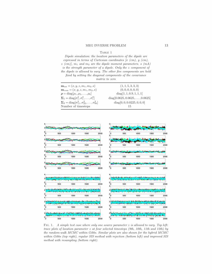
MEG INVERSE PROBLEM 13

Table 1

Dipole simulation: the location parameters of the dipole areexpressed in terms of Cartesian coordinates [x (cm), y (cm),

z (cm)], m1 and m2 are the dipole moment parameters. s (mA)is the strength parameter of a dipole. Only the z component ofthe dipole is allowed to vary. The other five components are held

fixed by setting the diagonal components of the covariancematrix to zero

mint = (x, y, z,m1,m2, s) (1,1,5,3,3,3)mcom = (x, y, z,m1,m2, s) (0,0,0,0,0,0)ρ= diag[ρ1, ρ2, . . . , ρ6] diag[1,1,0.9,1,1,1]

Σ1 = diag[σ21 , σ

21 , . . . , σ

21 ] diag[0.0625,0.0625, . . . ,0.0625]

Σ2 = diag[σ211, σ

222, . . . , σ

266] diag[0,0,0.0225,0,0,0]

Number of timesteps 15

Fig. 1. A simple test case where only one source parameter z is allowed to vary. Top left:trace plots of location parameter z at four selected timesteps (9th, 10th, 11th and 12th) bythe random-walk MCMC within Gibbs. Similar plots are also shown for the hybrid MCMCwithin Gibbs (top right), regular SIS method with rejection (bottom left) and improved SISmethod with resampling (bottom right).

14 Z. YAO AND W. F. EDDY

Table 2

Convergence diagnosis by effective sample size (ESS), Gelman–Rubin (GR) [Gelman andRubin (1992)]: value near 1 suggests convergence, Geweke (GE) [Geweke (1992)]:

z-score for stationary test, Heidelberger–Welch (HW) [Heidelberger and Welch (1983)]:p value for stationary test, Raftery–Lewis (RL) [Raftery and Lewis (1992)]: large value

suggests strong autocorrelation

Method ESS GR GE HW RL

Random-walk MCMC within Gibbs 26.7 1.29 −14.968 0.05 18.2Hybrid MCMC within Gibbs 553.5 1.06 −4.985 0.116 1.6Regular SIS with rejection 1946.9 1.013 −0.64 0.25 1.0Improved SIS with resampling 2000.0 1.005 −0.28 0.81 1.0

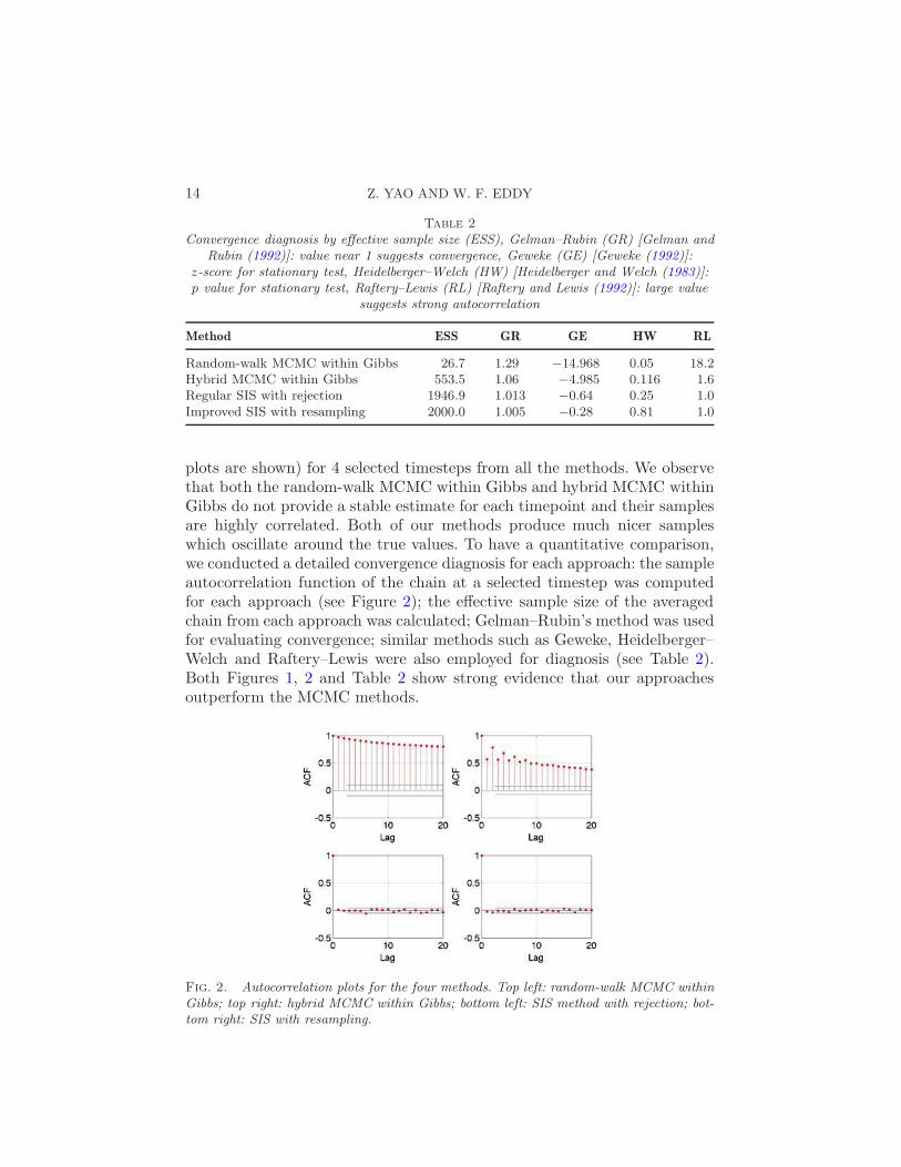
plots are shown) for 4 selected timesteps from all the methods. We observethat both the random-walk MCMC within Gibbs and hybrid MCMC withinGibbs do not provide a stable estimate for each timepoint and their samplesare highly correlated. Both of our methods produce much nicer sampleswhich oscillate around the true values. To have a quantitative comparison,we conducted a detailed convergence diagnosis for each approach: the sampleautocorrelation function of the chain at a selected timestep was computedfor each approach (see Figure 2); the effective sample size of the averagedchain from each approach was calculated; Gelman–Rubin’s method was usedfor evaluating convergence; similar methods such as Geweke, Heidelberger–Welch and Raftery–Lewis were also employed for diagnosis (see Table 2).Both Figures 1, 2 and Table 2 show strong evidence that our approachesoutperform the MCMC methods.

Fig. 2. Autocorrelation plots for the four methods. Top left: random-walk MCMC withinGibbs; top right: hybrid MCMC within Gibbs; bottom left: SIS method with rejection; bot-tom right: SIS with resampling.

MEG INVERSE PROBLEM 15

Table 3

Dipole simulation: the location parameters of the dipole areexpressed in terms of Cartesian coordinates [x (cm), y (cm),

z (cm)], m1 and m2 are the dipole moment parameters. s (mA) isthe strength parameter of a dipole. The diagonal elements of Σ1 and

Σ2 are 0.0625 fT2 and 0.01 cm2, respectively

Initial timepointmint = (x, y, z,m1,m2, s) (6,7,8,3,5,5)mcom = (x, y, z,m1,m2, s) (0,0,0,0,0,0)ρ=diag[ρ1, ρ2, . . . , ρ6] diag[0.65,0.7,0.75,0.8,0.85,0.9]

Random-walk move(x, y, z,m1,m2, s) Based on previous valueNumber of timesteps 10

Autoregressive move(x, y, z,m1,m2, s) Based on previous valuemcom = (x, y, z,m1,m2, s) (0,0,0,0,0,0)ρ=diag[ρ1, ρ2, . . . , ρ6] diag[0.65,0.7,0.75,0.8,0.85,0.9]

Random-walk move(x, y, z,m1,m2, s) Based on previous valueNumber of timesteps 10

· · · · · ·

Repeat until 100th timepoint

Simulated case 2. In addition to case 1, a case of multiple-source parame-ters (three location parameters and three moment and strength parameters)was performed. In this simulation, the source was modeled as a movingdipole following a multivariate autoregressive time series. The dipole movesin the three coordinate directions x, y and z, and both strength and mo-ments of the dipole change as well. The total length of simulation is 100timesteps (we will run 2000 timesteps for data in Section 4.3). To controlthe movement of the simulated dipole (to not move outside of the brainwhen the number of timepoints are large), we restricted the range of eachparameter for the dipole. In order to do this, we set boundary values for eachparameter (i.e., maximum and minimum). The autoregressive model for JP

t

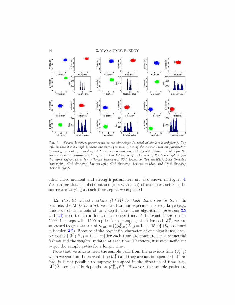
in Section 2 occurred only at certain timepoints when specified in advanced.In other words, the dipole had two types of moves: one is a move based onthe autoregressive model, and the other is a random-walk move. The dipolemoved according to the autoregressive model at certain specified timestepswhereas the random walk was applied to the dipole at the rest of the time-points. We had similar restrictions on the other parameters of the dipole.The parameters setup is given in Table 3. The plots (histogram) for eachdipole location parameter and pairwise plots for the location parametersare shown in Figure 3. These side by side histograms show the distributionof each location parameter at six selected timepoints. Similar plots for the

16 Z. YAO AND W. F. EDDY

Fig. 3. Source location parameters at six timesteps (a total of six 2× 2 subplots). Topleft: in this 2× 2 subplot, there are three pairwise plots of the source location parameters(x and y, x and z, y and z) at 1st timestep and one side by side histogram plot for thesource location parameters (x, y and z) at 1st timestep. The rest of the five subplots givethe same information for different timesteps: 20th timestep (top middle), 40th timestep(top right), 60th timestep (bottom left), 80th timestep (bottom middle) and 100th timestep(bottom right).

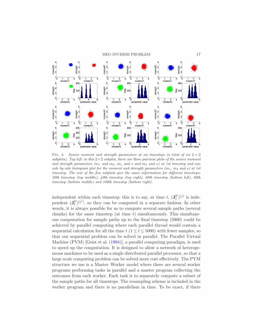
other three moment and strength parameters are also shown in Figure 4.We can see that the distributions (non-Gaussian) of each parameter of thesource are varying at each timestep as we expected.

4.2. Parallel virtual machine (PVM) for high dimension in time. Inpractice, the MEG data set we have from an experiment is very large (e.g.,hundreds of thousands of timesteps). The same algorithms (Sections 3.3and 3.4) need to be run for a much longer time. To be exact, if we run for5000 timesteps with 1500 replications (sample paths) for each JP

t , we aresupposed to get a stream of S5000 = (J P

5000)(j), j = 1, . . . ,1500 (St is defined

in Section 3.2). Because of the sequential character of our algorithms, sam-ple paths [(JP

t )(j), j = 1, . . . ,m] for each time are computed in a sequential

fashion and the weights updated at each time. Therefore, it is very inefficientto get the sample paths for a longer time.

Note that we always need the sample path from the previous time (JPt−1)

when we work on the current time (JPt ) and they are not independent, there-

fore, it is not possible to improve the speed in the direction of time [e.g.,(JP

t )(j) sequentially depends on (JP

t−1)(j)]. However, the sample paths are

MEG INVERSE PROBLEM 17

Fig. 4. Source moment and strength parameters at six timesteps (a total of six 2 × 2subplots). Top left: in this 2×2 subplot, there are three pairwise plots of the source momentand strength parameters (m1 and m2, m1 and s and m2 and s) at 1st timestep and oneside by side histogram plot for the moment and strength parameters (m1, m2 and s) at 1sttimestep. The rest of the five subplots give the same information for different timesteps:20th timestep (top middle), 40th timestep (top right), 60th timestep (bottom left), 80thtimestep (bottom middle) and 100th timestep (bottom right).

independent within each timestep; this is to say, at time t, (JPt )

(j) is inde-pendent (JP

t )(j′), so they can be computed in a separate fashion. In other

words, it is always possible for us to compute several sample paths (severalchunks) for the same timestep (at time t) simultaneously. This simultane-ous computation for sample paths up to the final timestep (5000) could beachieved by parallel computing where each parallel thread would contain asequential calculation for all the time t (1≤ t≤ 5000) with fewer samples, sothat our sequential problem can be solved in parallel. The Parallel VirtualMachine (PVM) [Geist et al. (1994)], a parallel computing paradigm, is usedto speed up the computation. It is designed to allow a network of heteroge-neous machines to be used as a single distributed parallel processor, so that alarge scale computing problem can be solved more cost effectively. The PVMstructure we use is a Master–Worker model where there are several workerprograms performing tasks in parallel and a master program collecting theoutcomes from each worker. Each task is to separately compute a subset ofthe sample paths for all timesteps. The resampling scheme is included in theworker program and there is no parallelism in time. To be exact, if there

18 Z. YAO AND W. F. EDDY

are three worker programs in the Master–Worker model to generate a steamST = (J P

T )(j), j = 1, . . . ,m, the way of running PVM is as follows:

Algorithm 2: PVM schedule

(i) Initialize each worker program and let each worker run for asubstream S′

T = (J PT )(j), j = 1, . . . , m3 .

(ii) Stack each S′T and get a complete ST .

The size of S′T can be adjusted according to the size of ST and the num-

ber of worker programs that are in use. The speed is mainly influenced byhardware and software components of network and I/O systems. It also de-pends on the number of worker programs, for example, adding too manyparallel workers does not enhance the speed when most of the time is spenton master–worker communication. In practice, deciding on the number ofworkers requires experience and it varies for different machines. Because themagnetic fields generated by independent dipoles add up, there is no addi-tional complexity (other than increased computation) brought by multipledipoles.

Since our PVM program involves randomness and a resampling scheme,several issues still need to be resolved. First, if our algorithms were imple-mented in a single program without parallelism, all samples generated beforeresampling from this program should be simply related to the random num-ber generator. However, when there are several workers, each of them doingthe same thing as a single program but in parallel, the unique randomnesswithin each worker will eventually come up with different but similar samplesbefore resampling. To be exact, in order to have the two programs generatethe same results, in the PVM structure we need to explicitly and preciselychoose different workers according to a predefined random sequence. Thisrandom sequence can be obtained from a single program without paral-lelism. Unfortunately, this needs a lot of work in programming and wouldsurely slow down the computation. Second, in a single program without par-allelism, we would only have one resampling procedure. The samples wouldbe generated from the resampling procedure. However, there would be oneresampling procedure within each of our worker programs in PVM. Thesamples would be generated from each of these workers and should eventu-ally be pooled together. In principle, the weights from each worker shouldbe pooled first and then we would perform the resampling procedure. Thereason is that each worker might generate different weights so that the nor-malizing constants might be different. If the resampling happens only onetime (at the end of all timesteps), a reasonable way to solve this problem isthat we can do the resampling scheme in the master program after normal-izing all the weights when pooled. If there were several resampling schemesbefore the end, we could still return to the master program when necessary.

MEG INVERSE PROBLEM 19

Again, this needs extensive programming and, again, it would surely slowdown the computations. In our current program, sums of weights withineach worker were almost the same (normalizing constants were almost thesame), so we retained the resampling procedure in each worker program.Because the random number generation will not produce the same numbersin a parallel program as in a sequential program without extensive inter-process communication and because resampling within each parallel workerprogram will produce different results than would resampling in the master,we do not expect the identical samples in the parallel version of our sequen-tial program. We do expect the distribution of the samples from the parallelprogram to be indistinguishable from the distribution of the samples fromthe sequential version.

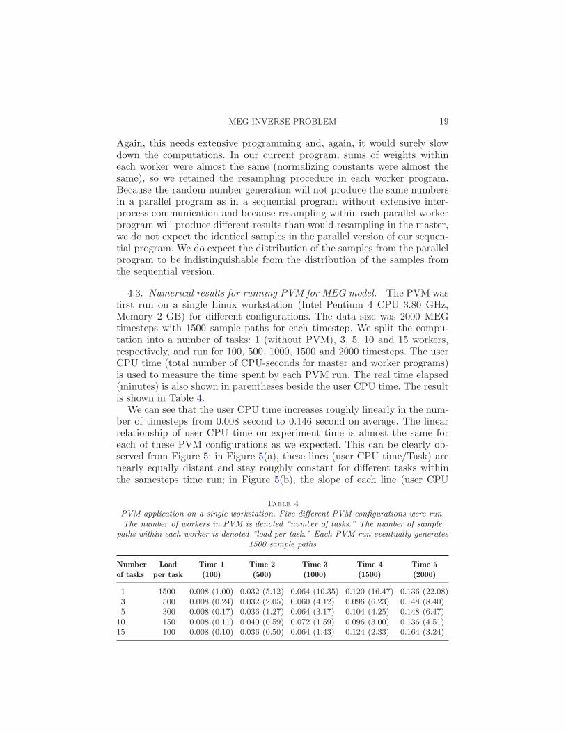
4.3. Numerical results for running PVM for MEG model. The PVM wasfirst run on a single Linux workstation (Intel Pentium 4 CPU 3.80 GHz,Memory 2 GB) for different configurations. The data size was 2000 MEGtimesteps with 1500 sample paths for each timestep. We split the compu-tation into a number of tasks: 1 (without PVM), 3, 5, 10 and 15 workers,respectively, and run for 100, 500, 1000, 1500 and 2000 timesteps. The userCPU time (total number of CPU-seconds for master and worker programs)is used to measure the time spent by each PVM run. The real time elapsed(minutes) is also shown in parentheses beside the user CPU time. The resultis shown in Table 4.

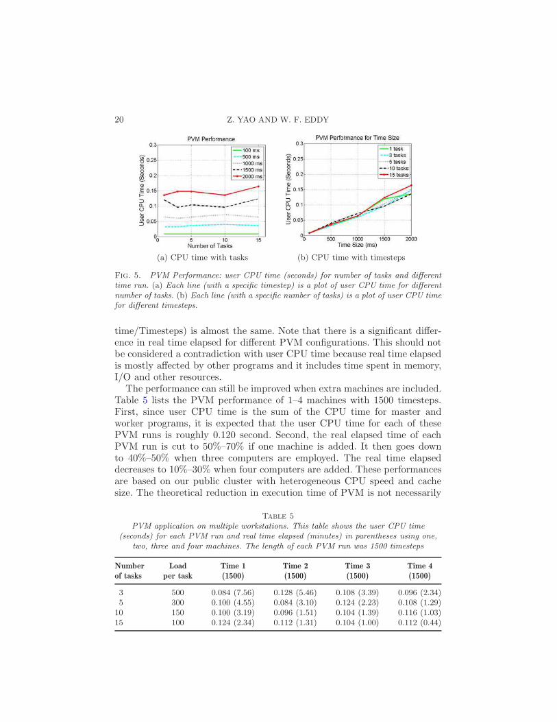
We can see that the user CPU time increases roughly linearly in the num-ber of timesteps from 0.008 second to 0.146 second on average. The linearrelationship of user CPU time on experiment time is almost the same foreach of these PVM configurations as we expected. This can be clearly ob-served from Figure 5: in Figure 5(a), these lines (user CPU time/Task) arenearly equally distant and stay roughly constant for different tasks withinthe samesteps time run; in Figure 5(b), the slope of each line (user CPU

Table 4

PVM application on a single workstation. Five different PVM configurations were run.The number of workers in PVM is denoted “number of tasks.” The number of sample

paths within each worker is denoted “load per task.” Each PVM run eventually generates1500 sample paths

Number Load Time 1 Time 2 Time 3 Time 4 Time 5of tasks per task (100) (500) (1000) (1500) (2000)

1 1500 0.008 (1.00) 0.032 (5.12) 0.064 (10.35) 0.120 (16.47) 0.136 (22.08)3 500 0.008 (0.24) 0.032 (2.05) 0.060 (4.12) 0.096 (6.23) 0.148 (8.40)5 300 0.008 (0.17) 0.036 (1.27) 0.064 (3.17) 0.104 (4.25) 0.148 (6.47)

10 150 0.008 (0.11) 0.040 (0.59) 0.072 (1.59) 0.096 (3.00) 0.136 (4.51)15 100 0.008 (0.10) 0.036 (0.50) 0.064 (1.43) 0.124 (2.33) 0.164 (3.24)

20 Z. YAO AND W. F. EDDY

(a) CPU time with tasks (b) CPU time with timesteps

Fig. 5. PVM Performance: user CPU time (seconds) for number of tasks and differenttime run. (a) Each line (with a specific timestep) is a plot of user CPU time for differentnumber of tasks. (b) Each line (with a specific number of tasks) is a plot of user CPU timefor different timesteps.

time/Timesteps) is almost the same. Note that there is a significant differ-ence in real time elapsed for different PVM configurations. This should notbe considered a contradiction with user CPU time because real time elapsedis mostly affected by other programs and it includes time spent in memory,I/O and other resources.

The performance can still be improved when extra machines are included.Table 5 lists the PVM performance of 1–4 machines with 1500 timesteps.First, since user CPU time is the sum of the CPU time for master andworker programs, it is expected that the user CPU time for each of thesePVM runs is roughly 0.120 second. Second, the real elapsed time of eachPVM run is cut to 50%–70% if one machine is added. It then goes downto 40%–50% when three computers are employed. The real time elapseddecreases to 10%–30% when four computers are added. These performancesare based on our public cluster with heterogeneous CPU speed and cachesize. The theoretical reduction in execution time of PVM is not necessarily

Table 5

PVM application on multiple workstations. This table shows the user CPU time(seconds) for each PVM run and real time elapsed (minutes) in parentheses using one,

two, three and four machines. The length of each PVM run was 1500 timesteps

Number Load Time 1 Time 2 Time 3 Time 4of tasks per task (1500) (1500) (1500) (1500)

3 500 0.084 (7.56) 0.128 (5.46) 0.108 (3.39) 0.096 (2.34)5 300 0.100 (4.55) 0.084 (3.10) 0.124 (2.23) 0.108 (1.29)

10 150 0.100 (3.19) 0.096 (1.51) 0.104 (1.39) 0.116 (1.03)15 100 0.124 (2.34) 0.112 (1.31) 0.104 (1.00) 0.112 (0.44)

MEG INVERSE PROBLEM 21

(a) Real time for PVM run (b) Total user CPU time for PVM run

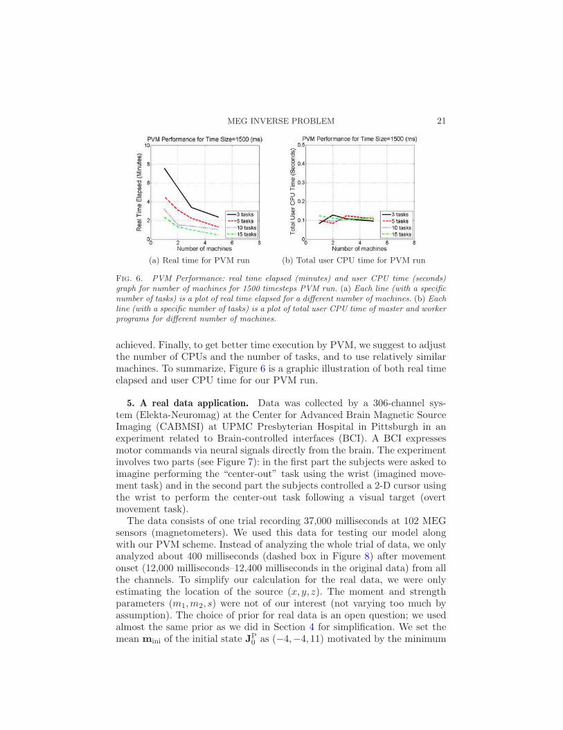
Fig. 6. PVM Performance: real time elapsed (minutes) and user CPU time (seconds)graph for number of machines for 1500 timesteps PVM run. (a) Each line (with a specificnumber of tasks) is a plot of real time elapsed for a different number of machines. (b) Eachline (with a specific number of tasks) is a plot of total user CPU time of master and workerprograms for different number of machines.

achieved. Finally, to get better time execution by PVM, we suggest to adjustthe number of CPUs and the number of tasks, and to use relatively similarmachines. To summarize, Figure 6 is a graphic illustration of both real timeelapsed and user CPU time for our PVM run.

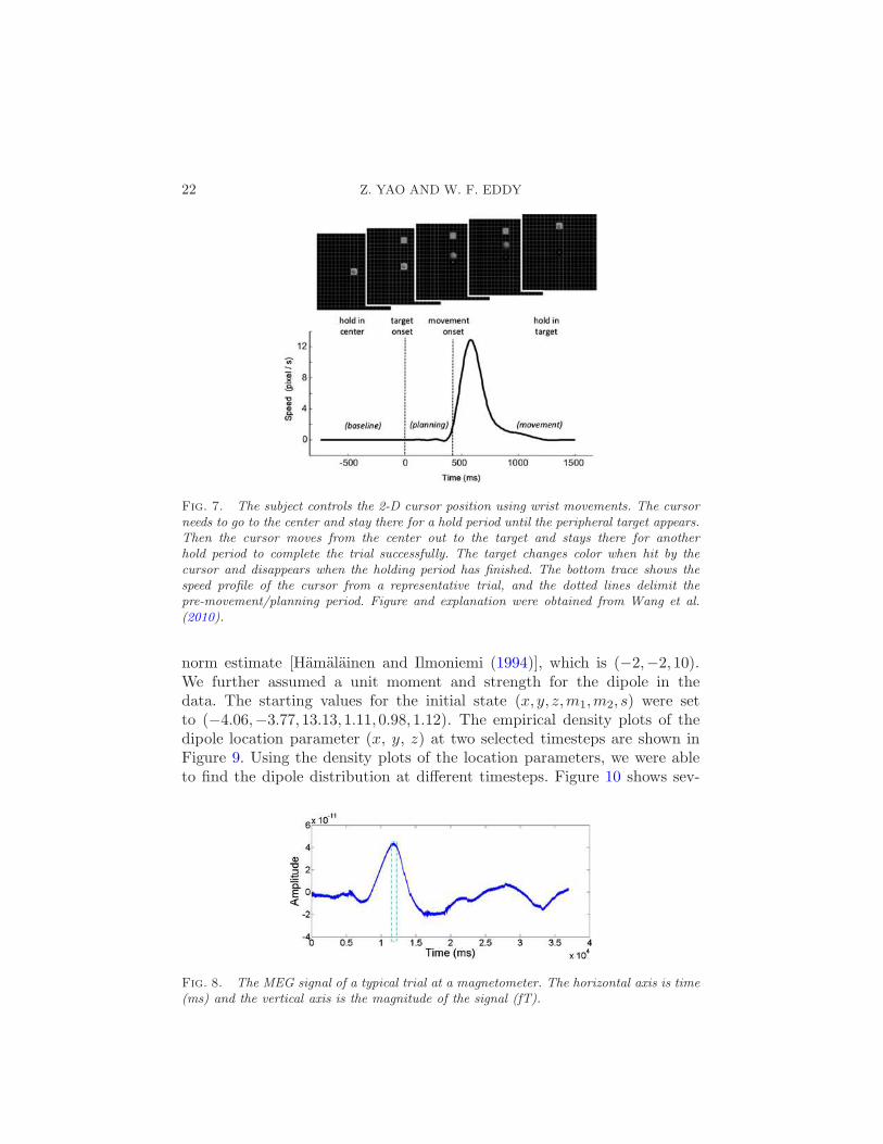
5. A real data application. Data was collected by a 306-channel sys-tem (Elekta-Neuromag) at the Center for Advanced Brain Magnetic SourceImaging (CABMSI) at UPMC Presbyterian Hospital in Pittsburgh in anexperiment related to Brain-controlled interfaces (BCI). A BCI expressesmotor commands via neural signals directly from the brain. The experimentinvolves two parts (see Figure 7): in the first part the subjects were asked toimagine performing the “center-out” task using the wrist (imagined move-ment task) and in the second part the subjects controlled a 2-D cursor usingthe wrist to perform the center-out task following a visual target (overtmovement task).

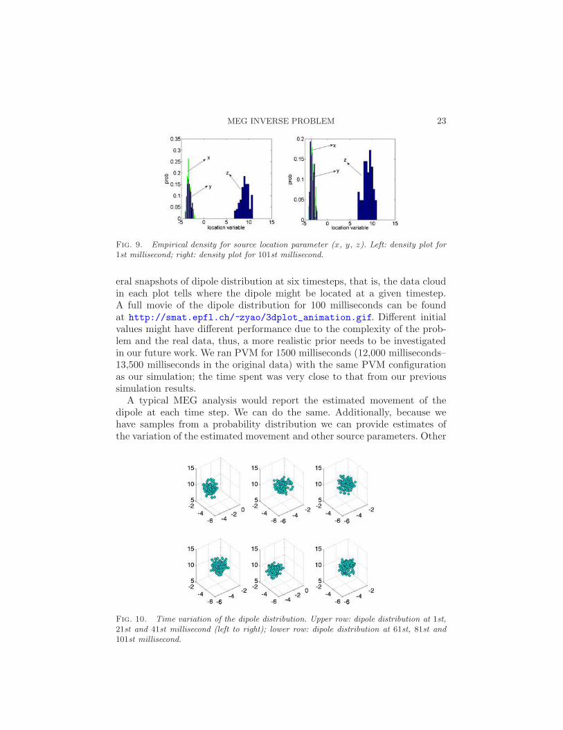
The data consists of one trial recording 37,000 milliseconds at 102 MEGsensors (magnetometers). We used this data for testing our model alongwith our PVM scheme. Instead of analyzing the whole trial of data, we onlyanalyzed about 400 milliseconds (dashed box in Figure 8) after movementonset (12,000 milliseconds–12,400 milliseconds in the original data) from allthe channels. To simplify our calculation for the real data, we were onlyestimating the location of the source (x, y, z). The moment and strengthparameters (m1,m2, s) were not of our interest (not varying too much byassumption). The choice of prior for real data is an open question; we usedalmost the same prior as we did in Section 4 for simplification. We set themean mini of the initial state JP

0 as (−4,−4,11) motivated by the minimum

22 Z. YAO AND W. F. EDDY

Fig. 7. The subject controls the 2-D cursor position using wrist movements. The cursorneeds to go to the center and stay there for a hold period until the peripheral target appears.Then the cursor moves from the center out to the target and stays there for anotherhold period to complete the trial successfully. The target changes color when hit by thecursor and disappears when the holding period has finished. The bottom trace shows thespeed profile of the cursor from a representative trial, and the dotted lines delimit thepre-movement/planning period. Figure and explanation were obtained from Wang et al.(2010).

norm estimate [Hamalainen and Ilmoniemi (1994)], which is (−2,−2,10).We further assumed a unit moment and strength for the dipole in thedata. The starting values for the initial state (x, y, z,m1,m2, s) were setto (−4.06,−3.77,13.13,1.11,0.98,1.12). The empirical density plots of thedipole location parameter (x, y, z) at two selected timesteps are shown inFigure 9. Using the density plots of the location parameters, we were ableto find the dipole distribution at different timesteps. Figure 10 shows sev-

Fig. 8. The MEG signal of a typical trial at a magnetometer. The horizontal axis is time(ms) and the vertical axis is the magnitude of the signal (fT).

MEG INVERSE PROBLEM 23

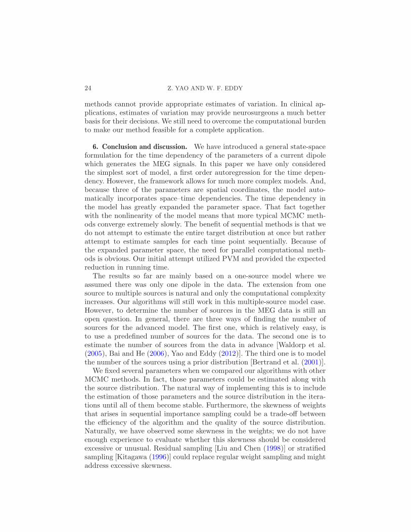
Fig. 9. Empirical density for source location parameter (x, y, z). Left: density plot for1st millisecond; right: density plot for 101st millisecond.

eral snapshots of dipole distribution at six timesteps, that is, the data cloudin each plot tells where the dipole might be located at a given timestep.A full movie of the dipole distribution for 100 milliseconds can be foundat http://smat.epfl.ch/~zyao/3dplot_animation.gif. Different initialvalues might have different performance due to the complexity of the prob-lem and the real data, thus, a more realistic prior needs to be investigatedin our future work. We ran PVM for 1500 milliseconds (12,000 milliseconds–13,500 milliseconds in the original data) with the same PVM configurationas our simulation; the time spent was very close to that from our previoussimulation results.

A typical MEG analysis would report the estimated movement of thedipole at each time step. We can do the same. Additionally, because wehave samples from a probability distribution we can provide estimates ofthe variation of the estimated movement and other source parameters. Other

Fig. 10. Time variation of the dipole distribution. Upper row: dipole distribution at 1st,21st and 41st millisecond (left to right); lower row: dipole distribution at 61st, 81st and101st millisecond.

24 Z. YAO AND W. F. EDDY

methods cannot provide appropriate estimates of variation. In clinical ap-plications, estimates of variation may provide neurosurgeons a much betterbasis for their decisions. We still need to overcome the computational burdento make our method feasible for a complete application.

6. Conclusion and discussion. We have introduced a general state-spaceformulation for the time dependency of the parameters of a current dipolewhich generates the MEG signals. In this paper we have only consideredthe simplest sort of model, a first order autoregression for the time depen-dency. However, the framework allows for much more complex models. And,because three of the parameters are spatial coordinates, the model auto-matically incorporates space–time dependencies. The time dependency inthe model has greatly expanded the parameter space. That fact togetherwith the nonlinearity of the model means that more typical MCMC meth-ods converge extremely slowly. The benefit of sequential methods is that wedo not attempt to estimate the entire target distribution at once but ratherattempt to estimate samples for each time point sequentially. Because ofthe expanded parameter space, the need for parallel computational meth-ods is obvious. Our initial attempt utilized PVM and provided the expectedreduction in running time.

The results so far are mainly based on a one-source model where weassumed there was only one dipole in the data. The extension from onesource to multiple sources is natural and only the computational complexityincreases. Our algorithms will still work in this multiple-source model case.However, to determine the number of sources in the MEG data is still anopen question. In general, there are three ways of finding the number ofsources for the advanced model. The first one, which is relatively easy, isto use a predefined number of sources for the data. The second one is toestimate the number of sources from the data in advance [Waldorp et al.(2005), Bai and He (2006), Yao and Eddy (2012)]. The third one is to modelthe number of the sources using a prior distribution [Bertrand et al. (2001)].

We fixed several parameters when we compared our algorithms with otherMCMC methods. In fact, those parameters could be estimated along withthe source distribution. The natural way of implementing this is to includethe estimation of those parameters and the source distribution in the itera-tions until all of them become stable. Furthermore, the skewness of weightsthat arises in sequential importance sampling could be a trade-off betweenthe efficiency of the algorithm and the quality of the source distribution.Naturally, we have observed some skewness in the weights; we do not haveenough experience to evaluate whether this skewness should be consideredexcessive or unusual. Residual sampling [Liu and Chen (1998)] or stratifiedsampling [Kitagawa (1996)] could replace regular weight sampling and mightaddress excessive skewness.

MEG INVERSE PROBLEM 25

To summarize, due to its nonuniqueness, finding a good estimate of theMEG source is a challenging problem which is still open. We have proposeda predictive model for finding a distribution for the MEG source and we haveapplied our methods on both simulated data and real data. In practice, theMEG data sets from different experimental settings are much more compli-cated. Our methods can be used as a reference with other source localizationmethods. Driven by the desire of looking at the brain activity in real time,we plan to implement a computing environment to study the brain activityunder the real MEG temporal resolution (1/1000 sec). The computationalchallenge arises due to the extremely large dimensionality of the problem(high resolution); there is no common computing architecture that couldhelp. We are exploring the use of more advanced forms of parallelism suchas CUDA (Compute Unified Device Architecture) and OPENCL to furtherreduce the running time in the future.

Acknowledgments. We thank Rob Kass and his collaborators for allow-ing us to use their BCI data to test our methods. Leon Gleser gave helpfulcomments on the paper. We thank the referee, the Area Editor and theEditor-in-Chief for their helpful comments. We are especially grateful tothe Associate Editor for his/her extremely helpful comments on versions ofthe manuscript and for his patience and persistence. We would also like tothank Dr. Alberto Sorrentino and Prof. Michele Piana of the Dipartimentodi Matematica, Universita di Genova for providing several references.

REFERENCES

Andrieu, C. and Thoms, J. (2008). A tutorial on adaptive MCMC. Stat. Comput. 18343–373. MR2461882

Bai, X. and He, B. (2006). Estimation of number of independent brain electric sourcesfrom the scalp EEGs. IEEE Trans. Biomed. Eng. 53 1883–1892.

Barkley, G. L. and Baumgartner, C. (2003). MEG and EEG in epilepsy. J. Clin.Neurophysiol. 20 163–178.

Bertrand, C., Ohmi, M., Suzuki, R. and Kado, H. (2001). A probabilistic solutionto the MEG inverse problem via MCMC methods: The reversible jump and paralleltempering algorithms. IEEE Trans. Biomed. Eng. 48 533–542.

Berzuini, C., Best, N. G., Gilks, W. R. and Larizza, C. (1997). Dynamic conditionalindependence models and Markov chain Monte Carlo methods. J. Amer. Statist. Assoc.92 1403–1412. MR1615251

Campi, C., Pascarella, A., Sorrentino, A. and Piana, M. (2008). A Rao–Blackwellized particle filter for magnetoencephalography. Inverse Problems 24 25023–25037.

Campi, C., Pascarella, A., Sorrentino, A. and Piana, M. (2011). Highly automateddipole estimation. Computational Intelligence and Neuroscience 2011 Article ID 982185,11 pp.

Carlin, B. P., Polson, N. G. and Stoffer, D. S. (1992). A Monte Carlo approach tononnormal and nonlinear state-space modeling. J. Amer. Statist. Assoc. 87 493–500.

26 Z. YAO AND W. F. EDDY

Carter, C. K. and Kohn, R. (1994). On Gibbs sampling for state space models.Biometrika 81 541–553. MR1311096

Cohen, D. (1968). Magnetoencephalography: Evidence of magnetic fields produced byalpha-rhythm currents. Science 161 784–786.

Del Moral, P., Doucet, A. and Jasra, A. (2006). Sequential Monte Carlo samplers.J. R. Stat. Soc. Ser. B Stat. Methodol. 68 411–436. MR2278333

Fearnhead, P. (2008). Computational methods for complex stochastic systems: A reviewof some alternatives to MCMC. Stat. Comput. 18 151–171. MR2390816

Gamerman, D. (1998). Markov chain Monte Carlo for dynamic generalised linear models.Biometrika 85 215–227. MR1627273

Geist, A., Beguelin, A., Dongarra, J., Jiang, W., Manchek, R. and Sun-

deram, V. S. (1994). PVM: Parallel Virtual Machine: A Users’ Guide and Tutorialfor Network Parallel Computing (Scientific and Engineering Computation). MIT Press,Cambridge, MA.

Gelman, A., Roberts, G. O. and Gilks, W. R. (1996). Efficient Metropolis jumpingrules. In Bayesian Statistics 599–607. Oxford Univ. Press, New York. MR1425429

Gelman, A. and Rubin, D. B. (1992). Inference from iterative simulation using multiplesequences. Statist. Sci. 7 457–511.

Geweke, J. (1992). Evaluating the accuracy of sampling-based approaches to the calcu-lation of posterior moments. In Bayesian Statistics 169–193. Oxford Univ. Press, NewYork. MR1380276

Gordon, N. J., Salmond, D. J. and Smith, A. F. M. (1993). Novel approach tononlinear/non-Gaussian Bayesian state estimation. IEE Proceedings F (Radar and Sig-nal Processing) 140 107–113.

Griffiths, D. J. (1999). Introduction to Electrodynamics. Prentice Hall, New York.Hamalainen, M. S. and Ilmoniemi, R. J. (1994). Interpreting magnetic fields of the

brain: Minimum norm estimates. Med. Biol. Eng. Comput. 32 35–42.Hamalainen, M. S., Hari, R., Ilmoniemi, R. J., Knuutila, J. and Lounasmaa, O. V.

(1993). Magnetoencephalography—theory, instrumentation, and applications to nonin-vasive studies of signal processing in the human brain. Rev. Modern Phys. 65 413–497.

Heidelberger, P. and Welch, P. D. (1983). Simulation run length control in the pres-ence of an initial transient. Oper. Res. 31 1109–1144.

Jun, S. C., George, J. S., Pare-Blagoev, J., Plis, S. M., Ranken, D. M.,Schmidt, D. M. and Wood, C. C. (2005). Spatiotemporal Bayesian inference dipoleanalysis for MEG neuroimaging data. NeuroImage 28 84–98.

Kitagawa, G. (1996). Monte Carlo filter and smoother for non-Gaussian nonlinear statespace models. J. Comput. Graph. Statist. 5 1–25. MR1380850

Knorr-Held, L. (1999). Conditional prior proposals in dynamic models. Scand. J. Stat.26 129–144.

Kristeva-Feige, R., Rossi, S., Feige, B., Mergner, Th., Lucking, C. H. andRossini, P. M. (1997). The bereitschaftspotential paradigm in investigating volun-tary movement organization in humans using magnetoencephalography (MEG). BrainRes. Protoc. 1 13–22.

Kybic, J., Clerc, M., Faugeras, O., Keriven, R. and Papadopoulo, T. (2006). Gen-eralized head models for MEG/EEG: Boundary element method beyond nested vol-umes. Phys. Med. Biol. 51 1333–1346.

Liu, J. S. (1996). Metropolized independent sampling with comparisons to rejection sam-pling and importance sampling. Statist. Comput. 6 113–119.

Liu, J. S. and Chen, R. (1998). Sequential Monte Carlo methods for dynamic systems.J. Amer. Statist. Assoc. 93 1032–1044. MR1649198

MEG INVERSE PROBLEM 27

Mattout, J., Phillips, C., Penny, W. D., Rugg, M. D. and Friston, K. J. (2006).MEG source localization under multiple constraints: An extended Bayesian framework.

NeuroImage 30 753–767.Miao, L., Michael, S., Kovvali, N., Chakrabarti, C. and Papandreou-

Suppappola, A. (2013). Multi-source neural activity estimation and sensor schedul-

ing: Algorithms and hardware implementation. Journal of Signal Processing Systems70 145–162.

Mosher, J. C., Lewis, P. S. and Leahy, R. M. (1992). Multiple dipole modeling andlocalization from spatio-temporal MEG data. IEEE Trans. Biomed. Eng. 39 541–557.

Neal, R. M. (2001). Annealed importance sampling. Stat. Comput. 11 125–139.

MR1837132Okada, Y., Lahteenmaki, A. and Xu, C. (1999). Comparison of MEG and EEG on the

basis of somatic evoked responses elicited by stimulation of the snout in the juvenileswine. Clin. Neurophysiol. 110 214–229.

Ou, W., Hamalainen, M. S. and Golland, P. (2009). A distributed spatio-temporal

EEG/MEG inverse solver. NeuroImage 44 932–946.Raftery, A. E. and Lewis, S. M. (1992). One long run with diagnostics: Implementation

strategies for Markov chain Monte Carlo. Statist. Sci. 7 493–497.Roberts, G. O. and Rosenthal, J. S. (2009). Examples of adaptive MCMC. J. Comput.

Graph. Statist. 18 349–367. MR2749836

Sarvas, J. (1984). Basic mathematical and electromagnetic concepts of the biomagneticinverse problem. Phys. Med. Biol. 32 11–22.

Schmidt, D. M., George, J. S. and Wood, C. C. (1999). Bayesian inference applied tothe electromagnet inverse problem. Hum. Brain Mapp. 7 195–212.

Shephard, N. and Pitt, M. K. (1997). Likelihood analysis of non-Gaussian measurement

time series. Biometrika 84 653–667. MR1603940Somersalo, E., Voutilainen, A. and Kaipio, J. P. (2003). Non-stationary magnetoen-

cephalography by Bayesian filtering of dipole models. Inverse Problems 19 1047–1063.MR2024688

Sorrentino, A., Parkkonen, L., Pascarella, A., Campi, C. and Piana, M. (2009).

Dynamical MEG source modeling with multi-target Bayesian filtering. Hum. BrainMapp. 30 1911–1921.

Sorrentino, A., Johansen, A. M., Aston, J. A. D., Nichols, T. E. andKendall, W. S. (2013). Dynamic filtering of static dipoles in magnetoencephalog-raphy. Ann. Appl. Stat. 7 955–988. MR3113497

Srinivasan, R. (2002). Importance Sampling: Applications in Communications and De-tection. Springer, Berlin. MR1949250

Uutela, K., Hamalainen, M. S. and Somersalo, E. (1999). Visualization of magne-toencephalographic data using minimum current estimates. NeuroImage 10 173–180.

Van Veen, B., Joseph, J. and Hecox, K. (1992). Localization of intra-cerebral sources of

electrical activity via linearly constrained minimum variance spatial filtering. In Proc.IEEE 6th SP Workshop on Statistical Signal and Array Processing 526–529. Victoria,

BC.Waldorp, L. J., Huizenga, H. M., Nehorai, A., Grasman, R. P. P. P. and Mole-

naar, P. C. M. (2005). Model selection in spatio-temporal electromagnetic source

analysis. IEEE Trans. Biomed. Eng. 52 414–420.Wang, W., Sudre, G. P., Xu, Y., Kass, R. E., Collinger, J. L., Degenhart, A. D.,

Bagic, A. I. and Weber, D. J. (2010). Decoding and cortical source localization forintended movement direction with MEG. J. Neurophysiol. 104 2451–2461.

28 Z. YAO AND W. F. EDDY

Yao, Z. and Eddy, W. F. (2012). Statistical approaches to estimating the number ofsignal sources in magnetoencephalography. Unpublished manuscript.

Section de Mathematiques

Ecole Polytechnique Federale de Lausanne

EPFL Station 8, 1015 Lausanne

Switzerland

E-mail: zhigang.yao@epfl.ch

Department of Statistics

Carnegie Mellon University

Pittsburgh, Pennsylvania 15213

USA

E-mail: bill@stat.cmu.edu