Inverse Problems in Transport Theory - MSRIlibrary.msri.org/books/Book47/files/stefanov.pdf ·...
21
Inside Out: Inverse Problems MSRI Publications Volume 47, 2003 Inverse Problems in Transport Theory PLAMEN STEFANOV Abstract. We study an inverse problem for the transport equation in a bounded domain in R n . Given the incoming flux on the boundary, we measure the outgoing one. The inverse problem is to recover the absorption coefficient σ a (x) and the collision kernel k(x, v 0 ,v) from this data. This paper is a survey of recent results about general k’s without assuming that k depends on a reduced number of variables. We present uniqueness results in dimensions n ≥ 3 for the time dependent and the stationary problem, and in the time dependent case we study the inverse scattering problem as well. The proofs are constructive and lead to direct procedures for recovering σ a and k. For n =2 the problem of recovering k is formally determined and we prove uniqueness for small k and a stability estimates. 1. Introduction This paper is a review of the recent progress in the study of inverse problems for the transport equation in R n , n ≥ 2 by the author and M. Choulli [CSt1], [CSt2], [CSt3], [CSt4] and the author and G. Uhlmann [StU]. We are focused here on the case when the collision kernel k introduced below depends on all of its variables x, v 0 , v. There are a lot of works dealing with k’s of the form k(x, v 0 · v) that is also physically important but we will not discuss those results here. Define the transport operator T by Tf = -v ·∇ x f (x, v) - σ a (x, v)f (x, v)+ Z V k(x, v 0 ,v)f (x, v 0 ) dv 0 , (1–1) where f = f (x, v) represents the density of a particle flow at the point x ∈ X moving with velocity v ∈ V . Here X ⊂ R n is a bounded domain with C 1 - boundary, V ⊂ R n is the velocity space. We assume that V is an open set in Sections 2 and 3, and that V = S n-1 (and dv is replaced by dS v ) in Section 4. All of our results in Sections 2 and 3 hold in the case when V = S n-1 with obvious modifications. In fact, the case V = S n-1 leads to some simplifications, The author was partly supported by NSF Grant DMS-0196440. 111
Transcript of Inverse Problems in Transport Theory - MSRIlibrary.msri.org/books/Book47/files/stefanov.pdf ·...
Inside Out: Inverse ProblemsMSRI PublicationsVolume 47, 2003
Inverse Problems in Transport Theory
PLAMEN STEFANOV
Abstract. We study an inverse problem for the transport equation in
a bounded domain in Rn. Given the incoming flux on the boundary, we
measure the outgoing one. The inverse problem is to recover the absorption
coefficient σa(x) and the collision kernel k(x, v′, v) from this data. This
paper is a survey of recent results about general k’s without assuming that
k depends on a reduced number of variables. We present uniqueness results
in dimensions n ≥ 3 for the time dependent and the stationary problem, and
in the time dependent case we study the inverse scattering problem as well.
The proofs are constructive and lead to direct procedures for recovering σa
and k. For n = 2 the problem of recovering k is formally determined and
we prove uniqueness for small k and a stability estimates.
1. Introduction
This paper is a review of the recent progress in the study of inverse problems
for the transport equation in Rn, n ≥ 2 by the author and M. Choulli [CSt1],
[CSt2], [CSt3], [CSt4] and the author and G. Uhlmann [StU]. We are focused
here on the case when the collision kernel k introduced below depends on all
of its variables x, v′, v. There are a lot of works dealing with k’s of the form
k(x, v′ · v) that is also physically important but we will not discuss those results
here.
Define the transport operator T by
Tf = −v · ∇xf(x, v) − σa(x, v)f(x, v) +
∫
V
k(x, v′, v)f(x, v′) dv′, (1–1)
where f = f(x, v) represents the density of a particle flow at the point x ∈ X
moving with velocity v ∈ V . Here X ⊂ Rn is a bounded domain with C1-
boundary, V ⊂ Rn is the velocity space. We assume that V is an open set in
Sections 2 and 3, and that V = Sn−1 (and dv is replaced by dSv) in Section 4.
All of our results in Sections 2 and 3 hold in the case when V = Sn−1 with
obvious modifications. In fact, the case V = Sn−1 leads to some simplifications,
The author was partly supported by NSF Grant DMS-0196440.
111
112 PLAMEN STEFANOV
for example there is no need to work locally in the open set V \ 0 in some
cases and the measure dξ can be chosen to be dξ in Section 3. The coefficient
σa(x, v) ≥ 0 above measures the absorption of particles at the point (x, v) due to
change of velocity or absorption by the surrounding media. The collision kernel
k(x, v′, v) ≥ 0 is related to the number of particles that change their velocity
from v′ to v at the point x.
We study inverse problems for both the time-dependent transport equation
(∂t − T )f = 0 (1–2)
and the stationary transport equation
Tf = 0. (1–3)
Set Γ± = (x, v) ∈ ∂X × V : ±n(x) · v > 0, where n(x) is the outer normal to
∂X at x ∈ ∂X. A typical boundary value problem for (1–2) or (1–3) is associated
with boundary conditions
f |Γ−= f−, (1–4)
where f− is a given function on Γ−, that depends also on t in the first case. On
the boundary we measure the outgoing flux f+ generated by a given incoming
flux f−, i.e., we assume that we know that so called albedo operator A defined
by
A : f− 7−→ f+ = f |Γ+. (1–5)
The inverse problem that we study is this: Can we determine the functions
σa and k from a knowledge of A? In the time dependent case we study the
inverse scattering problem as well — recovery of σa and k from the knowledge of
the scattering operator S. In order to ensure uniqueness of recovery of σa, we
assume that σa depends on x only, since otherwise there is clearly no uniqueness.
Under this assumption and some natural assumptions in the stationary case
that guarantee the solvability of the direct problem (1–2), we not only prove
uniqueness but give an explicit solution for the inverse problem. Our approach
is based on the study of the singularities of the Schwartz kernel of A and we
show that all information about σa and k is contained in those singularities. For
large σa, those singularities have very small amplitudes and are hard to measure
in real applications, so then this approach is of less interest for the practical
recovery of σa and k. In Section 4 we prove some stability estimates.
2. The Time Dependent Transport Equation
2.1. Main results In this section we present inverse problems results about
the time dependent transport equation (1–2)
∂
∂tu(x, v, t) = −v · ∇xu(x, v, t) − σa(x, v)u(x, v, t) +
∫
V
k(x, v′, v)u(x, v′, t) dv′.
(2–1)

INVERSE PROBLEMS IN TRANSPORT THEORY 113
We first introduce some terminology and notation. The production rate σp(x, v′)
is defined by
σp(x, v′) =
∫
V
k(x, v′, v) dv.
Following [RS] we say that the pair (σa, k) is admissible if
(i) 0 ≤ σa ∈ L∞(Rn × V ),
(ii) 0 ≤ k(x, v′, ·) ∈ L1(V ) for a.e. (x, v′) ∈ Rn × V and σp ∈ L∞(Rn × V ).
Throughout this paper we assume that σa and k are extended as 0 for x 6∈ X.
Set T0 = −v · ∇x with its maximal domain. It is well-known that T0 is a
generator of a strongly continuous group U0(t)f = f(x − tv, v) of isometries on
L1(X × V ) preserving nonnegative functions. Following the notation in [RS], we
introduce the operators
[A1f ](x, v) = −σa(x, v)f(x, v),
[A2f ](x, v) =
∫
V
k(x, v′, v)f(x, v′) dv′,
T1 = T0+A1,
T = T0+A1+A2
D(T1) = D(T0),
D(T ) = D(T0),
and set A = A1 + A2. Operators A1 and A2 are bounded on L1(X × V ) and
T1, T are generators of strongly continuous groups U1(t) = etT1 , U(t) = etT ,
respectively [RS]. For U1(t) we have an explicit formula
[U1(t)f ](x, v) = e−R
t
0σa(x−sv,v) dsf(x − tv, v), (2–2)
while for U(t) we have
‖U(t)‖ ≤ eCt, C = ‖σp‖L∞ . (2–3)
We work in the Banach space L1(X × V ), so here ‖U(t)‖ is the operator norm
of U(t) in L(L1(X × V )). It should be mentioned also that U(t) preserves the
cone of nonnegative functions for t ≥ 0.
One can define the wave operators associated with T , T0 by
W− = s-limt→∞
U(t)U0(−t), (2–4)
W+ = s-limt→∞
U0(−t)U(t). (2–5)
If W− and W+ exist, one can define the scattering operator
S = W+W−
as a bounded operator in L1(X × V ). Scattering theory for (1–1) has been devel-
oped in [Hej], [Si], [V1] and we refer to these papers (see also [RS]) for sufficient
conditions guaranteeing the existence of S. We would like to mention here also
[P1], [U], [E], [St], [V2], [CMS]. An abstract approach based on the Limiting
Absorption Principle has been proposed in [Mo]. We show below however that S
can always be defined as an operator S : L1c(R
n × V \0) → L1loc(R
n × V \0).

114 PLAMEN STEFANOV
The inverse scattering problem for (2–1) is the following: Does S determine
uniquely σa, k? The answer is affirmative if σa is independent of v.
Theorem 2.1 ([CSt1], [CSt2]). Let (σa, k), (σa, k) be two admissible pairs such
that σa, σa do not depend on v and denote by S, S the corresponding scattering
operators. Then, if S = S, we have σa = σa, k = k.
The assumption that σa, σa depend on x only can be relaxed a little by assuming
that they depend on x and |v| only. In the general case however, there is no
uniqueness. Assume, for example, that k = 0. Then
Sf = e−R
∞
−∞σa(x−sv,v) dsf, (k = 0) (2–6)
and therefore S determines∫ ∞
−∞σa(x − sv, v) ds only for any v ∈ V . It is easy
to see that those integrals do not determine σa uniquely. If σa is independent
of v/|v| however, then S determines the X-ray transform of σa and it therefore
determines σa in this case.
Next we consider the albedo operator A. Assume that X is convex and has
C1-smooth boundary ∂X. Consider the measure dξ = |n(x) · v|dµ(x) dv on Γ±,
where dµ(x) is the measure on ∂X. We will solve the problem
(∂t − T )u = 0 in R × X × V ,
u|R×Γ−= u−,
u|t0 = 0
(2–7)
for u(t, x, v), where u− ∈ L1c(R; L1(Γ−, dξ)). Problem (2–7) has a unique solu-
tion u ∈ C(R;L1(X × V )) and one defines the albedo operator A by
Ag = u|R×Γ+∈ L1
loc(R;L1(Γ+, dξ)). (2–8)
Therefore, A : L1c(R; L1(Γ−, dξ)) → L1
loc(R;L1(Γ+, dξ)). It can be seen that Ag
can be defined more generally for g ∈ L1(R×Γ−, dt dξ) with g = 0 for t 0. We
show below that in fact A determines S uniquely and conversely, S determines Auniquely by means of explicit formulae in case when X is convex. This generalizes
earlier results in [AE], [EP], [P2] showing that there is a relationship between S
and A. To this end, let us define the extension operators J± and the restriction
(trace) operators R± as follows. Set
Ω = (x, v) ∈ Rn × V \0 : x − tv ∈ X for some t ∈ R, (2–9)
and define the functions
τ±(x, v) = mint ∈ R : (x ± tv, v) ∈ Γ±, (x, v) ∈ Ω. (2–10)
Given g ∈ L1(R × Γ±, dt dξ), consider the following operators of extension:
(J±g)(x, v) =
g(
±τ±(x, v), x ± τ±(x, v)v, v)
if (x, v) ∈ Ω,
0 otherwise.

INVERSE PROBLEMS IN TRANSPORT THEORY 115
It is easy to check that J± : L1(R × Γ±, dt dξ) → L1(X × V ) are isometric.
Denote by R± the operator of restriction
R±f = f |Γ±, f ∈ C(Rn × V ).
Although R± is not a bounded operator on L1(X × V ) (see [Ce1], [Ce2] and
Theorem 3.2 below), we can show that R±U0(t)f ∈ L1(R × Γ±, dt dξ) is well
defined for any f ∈ L1(X × V ). Denote by χΩ the characteristic function of Ω.
We establish the following relationships between S and A.
Theorem 2.2 ([CSt1], [CSt2]). Assume that X is convex . Then
(a) Ag = R+U0(t)SJ−g for all g ∈ L1c(R × Γ−, dt dξ),
(b) Sf = J+AR−U0(t)f + (1 − χΩ)f , f ∈ L1c(R
n × V \0),(c) A extends to a bounded operator
A : L1(R × Γ−, dt dξ) → L1(R × Γ+, dt dξ)
if and only if S extends to a bounded operator on L1(X × V ).
We decompose L1(Rn × V ) = L1(Ω) ⊕ L1((Rn × V ) \ Ω). A similar decomposi-
tion holds for L1c(R
n × V \0). Then S leaves invariant both spaces, moreover
S|L1((Rn×V )\Ω) = Id, so S can be decomposed as a direct sum S = SΩ ⊕ Id.
Denote R± = R±U0( · ) : L1(Ω) → L1(R × Γ±, dt dξ). Then R± are iso-
metric and invertible and R−1± = J± with J± : L1(R × Γ±, dt dξ) → L1(Ω),
J±f := J±f |L1(Ω). Then we can rewrite Theorem 2.2 (a), (b) as follows:
A = R+SΩJ−
SΩ = J+AR−
on L1c(R × Γ−, dt dξ),
on L1c(R
n × V \0).
Thus A can be obtained from SΩ by a conjugation with invertible isometric
operators and vice-versa.
An immediate consequence of Theorem 2.2 is that A determines σa and k
uniquely for σa independent of v and X convex. In short, in this case the
inverse boundary value problem is equivalent to the inverse scattering problem.
However, we can prove uniqueness for the inverse boundary value problem for
not necessarily convex domains as well independently of Theorems 2.1 and 2.2.
Theorem 2.3 [CSt1], [CSt2]. Let (σa, k), (σa, k) be two admissible pairs with
σa, σa independent of v. Then, if the albedo operators A, A on ∂X coincide, we
have σa = σa, k = k.
2.2. Singular decomposition of the fundamental solution and the ker-
nels of S and A. Proof of the main results in section 2.1. The key to
proving the uniqueness results above is to study the singularities of the Schwartz
kernel of S and respectively A. To this end we will study first the kernel of the
116 PLAMEN STEFANOV
solution operator of the problem (2–7). Given (x′, v′) ∈ Rn × V \0, consider
the problem
(∂t − T )u = 0 in R × Rn × V ,
u|t0 = δ(x − x′ − tv)δ(v − v′),(2–11)
δ being the Dirac delta function. Problem (2–1) has a unique solution
u#(t, x, v, x′, v′)
depending continuously on t with values in D′(Rnx × Vv × R
nx′ × Vv′\0). We
have the following singular expansion of u#.
Theorem 2.4 [CSt1], [CSt2]. Problem (2–11) has the unique solution u# =
u#0 + u#
1 + u#2 , where
u#0 = e−
R
∞
0σa(x−sv,v) dsδ(x − x′ − tv)δ(v − v′),
u#1 =
∫ ∞
0
e−R
s
0σa(x−τv,v)dτe−
R
∞
0σa(x−sv−τv′,v′)dτ
× k(x−sv, v′, v)δ(x − sv − (t−s)v′ − x′) ds,
u#2 ∈ C
(
R; L∞loc(R
nx′ × Vv′ ; L1(Rn
x × Vv)))
.
The proof of Theorem 2.4 is based on iterating twice Duhamel’s formula
U(t − r) = U1(t − r) +
∫ t
r
U(t − s)A2U1(s − r) ds
and on estimating the remainder term.
To build the scattering theory for the transport equation, we first show that
the wave operators W−, W+ (see (2–4), (2–5)) exist as operators between the
spaces
W− : L1c(R
n × V \0) −→ L1(X × V ),
W+ : L1(X × V ) −→ L1loc(R
n × V \0).Then we define the scattering operator
S = W+W− : L1c(R
n × V \0) −→ L1loc(R
n × V \0). (2–12)
It can be seen that S is well defined on the wider subset
f : ∃t0 such that
U0(t)f = 0 for x ∈ X, t < −t0
(the incoming space).
The distribution u#(t, x, v, x′, v′) is the Schwartz kernel of U(t)W−. Let
S(x, v, x′, v′) be the Schwartz kernel of the scattering operator S. Then
S(x, v, x′, v′) = limt→∞
u#(t, x+tv, v, x′, v′).
This limit exists trivially, in fact for any K b Rn × V \0, the distribution
u#(t, x+tv, v, x′, v′)|K is independent of t for t ≥ t0(K). On the other hand,
as mentioned in the Introduction, it is not trivial to show that under some

INVERSE PROBLEMS IN TRANSPORT THEORY 117
condition, S is a kernel of a bounded operator in L1(Rn × V ). One can also
prove the following integral representation of the scattering kernel:
S(x, v, x′, v′) = e−R
∞
−∞σa(x−τv,v)dτδ(x − x′)δ(v − v′)
+
∫ ∞
−∞
e−R
∞
sσa(x+τv,v)dτ (A2u
#)(s, x + sv, v, x′, v′) ds. (2–13)
This formula is an analogue of the representation of the scattering amplitude (in
our setting, that would be the second term in the right-hand side above) for the
Schrödinger equation.
Now, combining Theorem 2.4 and the representation above, we get the fol-
lowing express for the kernel S of the scattering operator S.
Theorem 2.5 [CSt1], [CSt2]. We have S = S0 + S1 + S2, where the Schwartz
kernels Sj(x, v, x′, v′) of the operators Sj , j = 0, 1, 2 satisfy
S0 = e−R
∞
−∞σa(x−τv,v)dτ δ(x − x′)δ(v − v′),
S1 =
∫ ∞
−∞
e−R
∞
sσa(x+τv,v)dτe−
R
∞
0σa(x+sv−τv′,v′)dτ
k(x + sv, v′, v)δ(x − x′ + s(v − v′)) ds,
S2 ∈ L∞loc(R
nx′ × Vv′\0; L1
loc(Rnx × Vv\0)).
We are ready now to complete the proof of Theorem 2.1. The idea of the proof is
the following. Suppose we are given the scattering operator S corresponding to
a unknown admissible pair (σa, k). Then we know the kernel S = S0 + S1 + S2.
It follows from Theorem 2.5 that S0 is a singular distribution supported on the
hyperplane x = x′, v = v′ of dimension 2n, S1 is supported on a (3n + 1)-
dimensional surface (for v 6= v′), while S2 is a function. Therefore, Sj , j = 0, 1, 2
have different degrees of singularities and given S = S0 + S1 + S2, one can
always recover S0 and S1. From S0 one can recover the X-ray transform of σa
and therefore σa itself, provided that σa is independent of v. Next, suppose for
simplicity that σa and k are continuous. Then for fixed x, v, v′ with v 6= v′, S1
is a delta-function supported on the line x′ = x + s(v − v′), s ∈ R with density
a multiple of k(x + sv, v′, v). Therefore, one can recover that density for each s
and in particular setting s = 0, we get k(x, v′, v). Moreover, based on this, we
can write explicit formulae that extract σa and k from S by allowing S to act
on a sequence of suitably chosen test functions that concentrate on one of the
singular varieties described above, see [CSt2].
We will skip the proof of Theorem 2.2. We merely recall that it proves unique-
ness for the inverse boundary value problem for convex X as a direct consequence
of Theorem 2.5.
Now assume that X is not necessarily convex. We can still prove uniqueness
for the inverse boundary value problem by showing that A determines uniquely
u# for x outside X by following arguments in [SyU], and then using (2–13) and
Theorem 2.5. In order to give a constructive (in fact, explicit) reconstruction, we

118 PLAMEN STEFANOV
study next the Schwartz kernel of the operator A in the spirit of Theorem 2.5.
A priori, this kernel is a distribution in D′(R ×Γ+ ×R ×Γ−). Denote by δ1 the
Dirac delta function on R1 and by δy(x) the Delta function on ∂X defined by
∫
∂Xδyϕdµ(x) = ϕ(y). Set
θ(x, y) =
1 if px + (1 − p)y ∈ X for each p ∈ [0, 1],
0 otherwise.
Theorem 2.6 [CSt1], [CSt2]. The Schwartz kernel of A has the form
α(t − t′, x, v, x′, v′),
that is, formally ,
(Ag)(t, x, v) =
∫
R×Γ−
α(t − t′, x, v, x′, v′)g(t′, x′, v′) dξ(x′, v′)
with α = α0+α1+α2, where the αj(τ, x, v, x′, v′) (with (x, v) ∈ Γ+, (x′, v′) ∈ Γ−)
satisfy
α0 = |n(x′)·v′|−1e−R τ−(x,v)
0 σa(x−sv,v) dsδx−τ−(x,v)v(x′)δ(v−v′)δ1(τ−τ−(x, v)),
α1 = |n(x′)·v′|−1
∫
e−R
s
0σa(x−pv,v) dpe−
R τ−(x−sv,v′)
0 σa(x−sv−pv′,v′) dp×δ1(τ−s−τ−(x−sv, v′))k(x−sv, v′, v)δx−sv−τ−(x−sv,v′)v′(x
′)θ(x−sv, x) ds,
α2 ∈ L∞(
Γ−; L1loc(Rτ ; L1(Γ+, dξ))
)
.
The proof of Theorem 2.3 now follows from the theorem above by analyzing the
singularities of α as above. In this case, we can also wite explicit formulae for σa
and k as certain limits of the distribution α acting on a sequence of test functions
concentrating near the singularities of α0 and α1, respectively; see [CSt2].
3. The Stationary Transport Equation
We turn our attention now to the boundary value problem (1–3), (1–4) for
the stationary transport equation
−v · ∇xf(x, v) − σa(x, v)f(x, v) +
∫
V
k(x, v′, v)f(x, v′) dv′ = 0 in X × V ,
f |Γ−= f−. (3–1)
Here X does not need to be convex. We impose some conditions in order to
ensure the unique solvability of the direct problem (3–1). Recall the definition
(2–10) of τ±. Set τ = τ− + τ+. We will consider two cases. First we assume that
‖τσa‖L∞ < ∞, ‖τσp‖L∞ < 1. (3–2)
This condition in particular guarantees that the dynamics U(t) corresponding to
the time-dependent transport equation (∂t −T )u = 0 is subcritical [RS], that is,
the L1-norm of the solution is uniformly bounded for t > 0; compare with (2–3).

INVERSE PROBLEMS IN TRANSPORT THEORY 119
Note that (3–2) holds if in particular∥
∥|v|−1σa
∥
∥
L∞ < ∞, diamX∥
∥|v|−1σp
∥
∥
L∞ <
1. The second situation we will consider is when [DL]
0 ≤ ν ≤ σa(x, v) − σp(x, v) for a.e. (x, v) ∈ X × V (3–3)
with some ν > 0. This condition means that the absorption rate is greater
than the production rate. This also implies that the corresponding dynamics is
subcritical.
The main result in this section is this:
Theorem 3.1 [CSt3], [CSt4]. Assume that (σa, k), (σa, k) are two admissible
pairs with σa = σa(x, |v|), σa = σa(x, |v|) and assume that they satisfy either
(3–2) or (3–3). Assume that the corresponding albedo operators A and A coin-
cide. Then
(a) if n ≥ 3, then σa = σa, k = k;
(b) if n = 2, then σa = σa.
In the stationary case we have less data than in the time dependent one studied
in Section 2 because the time variable is not present. The inverse boundary value
problem is overdetermined in dimension n ≥ 3 because the kernel of A depends
on 4n−2 variables while k is a function of 3n variables, σa(x, v/|v|) is a function
of 2n − 1 variables. In the 2D case however, the inverse problem for recovery of
k is formally determined (but still overdetermined for the recovery of σa) and
the theorem above does not provide uniqueness in this case. In Section 4 we
formulate a uniqueness result in the 2D case for small k.
To prove Theorem 3.1, we again study the Schwartz kernel of the albedo
operator A. Note that in the stationary case, A acts on functions on Γ− and
maps them to functions on Γ+ (see next subsection for details). It turns out that,
similarly to the time dependent case, the kernel of A has a singular decomposition
α = α0 + α1 + α2, where α0 and α1 are delta functions for n ≥ 3 supported on
varieties of different dimensions with densities that identify respectively σa and
k. The third term α2 is a locally L1 function and can be distinguished form α0
and α1. If n = 2, α0 is still a delta function, but α1 is a locally L1 function and
cannot be distinguished from α2 and this explains why this method does not
work then. The 2D case is considered separately in next section.
3.1. Some estimates in the stationary case Similarly to the measure
defined in Section 2.1, we define a measure on Γ± by:
dξ = minτ(x, v), λ∣
∣n(x) · v∣
∣ dµ(x) dv,
where λ > 0 is an arbitrary constant. Using the trace Theorem 3.2 below, we can
show that A : L1(Γ−, dξ) → L1(Γ+, dξ) is a bounded operator if (3–2) holds and
A : L1(Γ−, dξ) → L1(Γ+, dξ) is bounded if (3–3) holds; see also [DL]. Note that
if a neighborhood of the origin is not included in V or in particular, if V = Sn−1,
then we can choose dξ = τdξ.
120 PLAMEN STEFANOV
Theorem 3.2 (Trace theorem). (a) [CSt3]∥
∥f |Γ±
∥
∥
L1(Γ±,dξ)≤ ‖T0f‖ + ‖τ−1f‖.
(b) [Ce1], [Ce2]∥
∥f |Γ±
∥
∥
L1(Γ±,dξ)≤ λ‖T0f‖ + ‖f‖.
Note that (b) follows from (a) by setting f = minλ, τg.
We introduce the spaces W, W via the norms
‖f‖W = ‖T0f‖ + ‖τ−1f‖, ‖f‖W = ‖T0f‖ + ‖f‖.
Then Theorem 3.2 says that taking the trace f 7→ f |Γ±is a continuous operator
from W into L1(Γ±, dξ) and similarly from W into L1(Γ±, dξ).
Given f− ∈ L1(Γ−, dξ), define Jf− as the following prolongation of f− inside
X × V :
Jf− = e−R τ−(x,v)
0 σa(x−sv,v) dsf−(x − τ−(x, v)v, v), (x, v) ∈ X × V .
Jf− is defined so that T1Jf− = 0, Jf−|Γ−= f−, therefore J is the solution
operator of the problem T1f = 0, f |Γ−= f−.
Proposition 3.1. (a) Assume that ‖τσa‖L∞ < ∞. Then
‖Jf−‖W ≤ C‖f−‖L1(Γ−,dξ),
with C = 1 + ‖τσa‖L∞ . If σa = 0, then we have equality above (and C = 1).
(b) Assume (3–3). For any f− ∈ L1(Γ−, dξ) we have
‖Jf−‖W ≤ C‖f−‖L1(Γ−,dξ),
where C = (1 + ‖σa‖L∞)max1, (νλ)−1.
We reduce the boundary value problem (3–1) to an integral equation using stan-
dard arguments to get
(I + K)f = Jf−, (3–4)
where I stands for the identity and K is the integral operator
Kf = −∫ τ−(x,v)
0
e−R
t
0σa(x−sv,v) ds(A2f)(x − tv, v) dt. (3–5)
Formally, K = T−11 A2, and for T−1
1 we have
T−11 f = −
∫ τ−(x,v)
0
e−R
t
0σa(x−sv,v) dsf(x − tv, v) dt.
Proposition 3.2. Assume (3–2). Then:
(a) τ−1T−11 , τ−1T−1 and A2τ are bounded operators in L1(X × V ) and therefore
K = T−11 A2 is a bounded operator in L1(X × V ; τ−1 dx dv). Moreover , the
operator norm of K is not greater than ‖τσp‖L∞ < 1 and therefore (I +K)−1
exists in this space.
INVERSE PROBLEMS IN TRANSPORT THEORY 121
(b) The integral equation (3–4) and therefore the boundary value problem (3–1)
are uniquely solvable for any f− ∈ L1(Γ−, dξ) and then f ∈ W.
(c) The albedo operator A is a bounded map A : L1(Γ−, dξ) → L1(Γ+, dξ).
Proposition 3.3. Assume (3–3). Then:
(a) K, T−11 and T−1 are bounded operators in L1(X × V ) and K = T−1
1 A2.
Further , I + K is invertible and (I + K)−1 = I − T−1A2.
(b) The integral equation (3–4) and therefore the boundary value problem (3–1)
are uniquely solvable for any f− ∈ L1(Γ−, dξ) and then f ∈ W.
(c) A is a bounded map A : L1(Γ−, dξ) → L1(Γ+, dξ).
3.2. The fundamental solution of the stationary transport equation.
We solve (3–1) with f− = φ−, where
φ− =1
|n(x′) · v′|δx′(x)δ(v − v′),
where (x′, v′) ∈ Γ− are regarded as parameters, n(x′) is the outer normal, and
δx′ is a distribution on ∂X defined by (δx′, ϕ) =∫
δx′(x)ϕ(x)dµ(x) = ϕ(x′).
On the other hand, we will denote by δ the ordinary Dirac delta function in Rn.
The integral above is to be considered in distribution sense. Let us denote by
φ(x, v, x′, v′) the solution (in distribution sense) of
Tφ = 0 in X × V ,
φ|Γ−= φ−.
(3–6)
To solve (3–6), we write
ϕ = Jϕ− − KJϕ− + (I + K)−1K2Jϕ−
and analyze each term. To treat the third term, we observe that
(I + K)−1K2Jϕ− = T−1A2KJϕ−.
We are led to:
Theorem 3.3. Assume that (σa, k) is admissible and either (3–2) or (3–3) holds.
Then the solution φ(x, v, x′, v′) of (3–6) can be written as φ = φ0+φ1+φ2, where
φ0 =
∫ τ+(x′,v′)
0
e−R τ−(x,v)
0 σa(x−pv,v) dpδ(x − x′ − tv)δ(v − v′) dt,
φ1 =
∫ τ−(x,v)
0
∫ τ+(x′,v′)
0
e−R
s
0σa(x−pv,v) dpe−
R τ−(x−sv,v′)
0 σa(x−sv−pv′,v′) dp
× k(x − sv, v′, v)δ(x − x′ − sv − tv′) dt ds,
andφ2 ∈ L∞(Γ−; W) if (3–2) holds,
minτ, λ−1φ2 ∈ L∞(Γ−; W) if (3–3) holds.
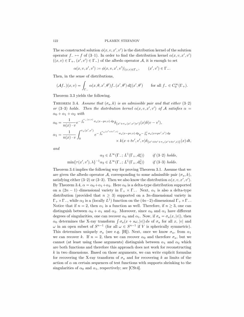
122 PLAMEN STEFANOV
The so constructed solution φ(x, v, x′, v′) is the distribution kernel of the solution
operator f− 7→ f of (3–1). In order to find the distribution kernel α(x, v, x′, v′)
((x, v) ∈ Γ+, (x′, v′) ∈ Γ−) of the albedo operator A, it is enough to set
α(x, v, x′, v′) := φ(x, v, x′, v′)|(x,v)∈Γ+, (x′, v′) ∈ Γ−.
Then, in the sense of distributions,
(Af−)(x, v) =
∫
Γ−
α(x, θ, x′, θ′)f−(x′, θ′) dξ(x′, θ′) for all f− ∈ C∞0 (Γ+).
Theorem 3.3 yields the following.
Theorem 3.4. Assume that (σa, k) is an admissible pair and that either (3–2)
or (3–3) holds. Then the distribution kernel α(x, v, x′, v′) of A satisfies α =
α0 + α1 + α2 with
α0 =1
n(x) · v e−R τ−(x,v)
0 σa(x−pv,v) dpδx′+τ+(x′,v′)v′(x)δ(v − v′),
α1 =1
n(x) · v
∫ τ+(x′,v′)
0
e−R τ+(x′+tv′,v)
0 σa(x−pv,v) dpe−R
t
0σa(x+pv′,v′) dp
× k(x + tv′, v′, v)δx′+tv′+τ+(x′+tv′,v)(x) dt,
and
α2 ∈ L∞(Γ−; L1(Γ+, dξ)) if (3–2) holds,
minτ(x′, v′), λ−1α2 ∈ L∞(Γ−; L1(Γ+, dξ)) if (3–3) holds.
Theorem 3.4 implies the following way for proving Theorem 3.1. Assume that we
are given the albedo operator A, corresponding to some admissible pair (σa, k),
satisfying either (3–2) or (3–3). Then we also know the distribution α(x, v, x′, v′).
By Theorem 3.4, α = α0+α1+α2. Here α0 is a delta-type distribution supported
on a (2n − 1)–dimensional variety in Γ+ × Γ−. Next, α1 is also a delta-type
distribution (provided that n ≥ 3) supported on a 3n-dimensional variety in
Γ+×Γ−, while α2 is a (locally L1) function on the (4n−2)-dimensional Γ+×Γ−.
Notice that if n = 2, then α1 is a function as well. Therefore, if n ≥ 3, one can
distinguish between α0 + α1 and α2. Moreover, since α0 and α1 have different
degrees of singularities, one can recover α0 and α1. Now, if σa = σa(x, |v|), then
α0 determines the X-ray transform∫
σa(x + sω, |v|) ds of σa for all x, |v| and
ω in an open subset of Sn−1 (for all ω ∈ Sn−1 if V is spherically symmetric).
This determines uniquely σa (see e.g. [H]). Next, once we know σa, from α1
we can recover k. If n = 2, then we can recover α0 and therefore σa, but we
cannot (at least using those arguments) distinguish between α1 and α2 which
are both functions and therefore this approach does not work for reconstructing
k in two dimensions. Based on those arguments, we can write explicit formulas
for recovering the X-ray transform of σa and for recovering k as limits of the
action of α on certain sequences of test functions with supports shrinking to the
singularities of α0 and α1, respectively; see [CSt4].
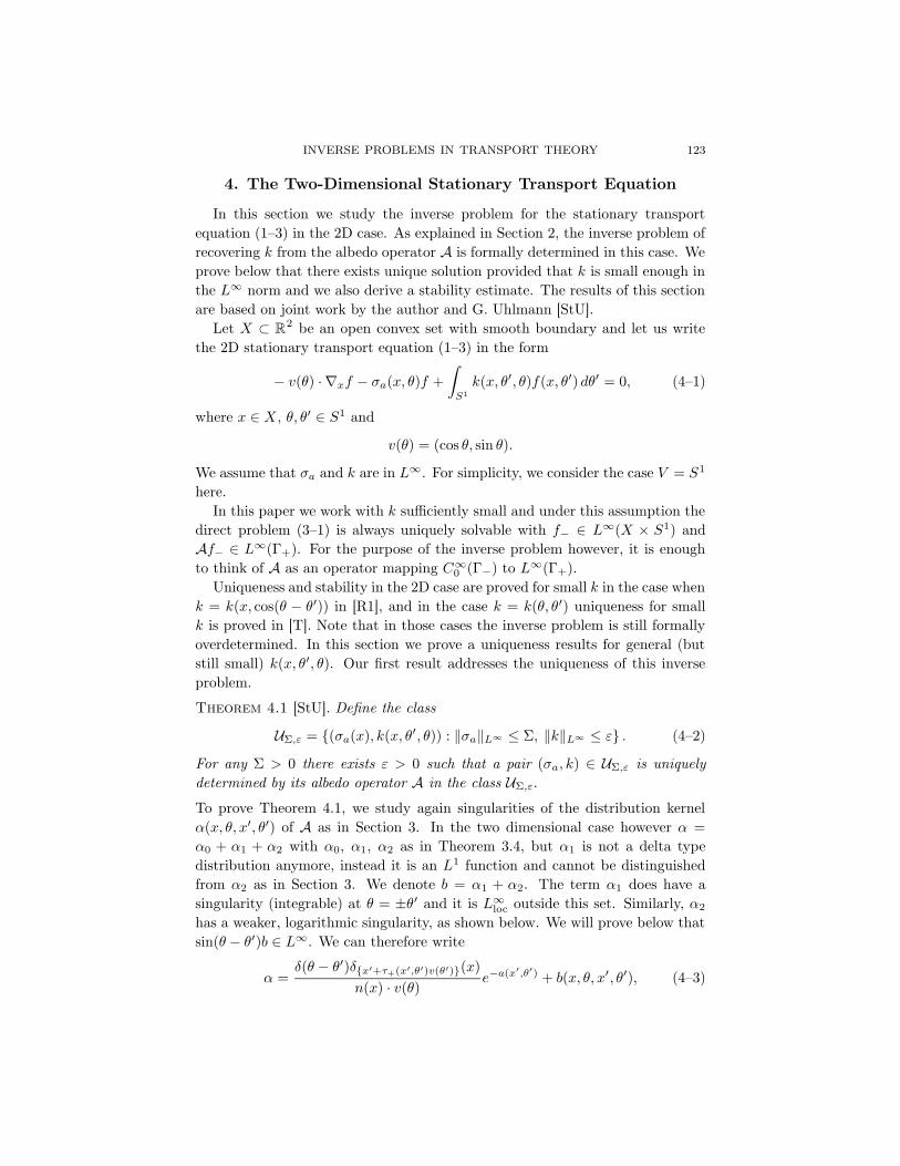
INVERSE PROBLEMS IN TRANSPORT THEORY 123
4. The Two-Dimensional Stationary Transport Equation
In this section we study the inverse problem for the stationary transport
equation (1–3) in the 2D case. As explained in Section 2, the inverse problem of
recovering k from the albedo operator A is formally determined in this case. We
prove below that there exists unique solution provided that k is small enough in
the L∞ norm and we also derive a stability estimate. The results of this section
are based on joint work by the author and G. Uhlmann [StU].
Let X ⊂ R2 be an open convex set with smooth boundary and let us write
the 2D stationary transport equation (1–3) in the form
− v(θ) · ∇xf − σa(x, θ)f +
∫
S1
k(x, θ′, θ)f(x, θ′) dθ′ = 0, (4–1)
where x ∈ X, θ, θ′ ∈ S1 and
v(θ) = (cos θ, sin θ).
We assume that σa and k are in L∞. For simplicity, we consider the case V = S1
here.
In this paper we work with k sufficiently small and under this assumption the
direct problem (3–1) is always uniquely solvable with f− ∈ L∞(X × S1) and
Af− ∈ L∞(Γ+). For the purpose of the inverse problem however, it is enough
to think of A as an operator mapping C∞0 (Γ−) to L∞(Γ+).
Uniqueness and stability in the 2D case are proved for small k in the case when
k = k(x, cos(θ − θ′)) in [R1], and in the case k = k(θ, θ′) uniqueness for small
k is proved in [T]. Note that in those cases the inverse problem is still formally
overdetermined. In this section we prove a uniqueness results for general (but
still small) k(x, θ′, θ). Our first result addresses the uniqueness of this inverse
problem.
Theorem 4.1 [StU]. Define the class
UΣ,ε = (σa(x), k(x, θ′, θ)) : ‖σa‖L∞ ≤ Σ, ‖k‖L∞ ≤ ε . (4–2)
For any Σ > 0 there exists ε > 0 such that a pair (σa, k) ∈ UΣ,ε is uniquely
determined by its albedo operator A in the class UΣ,ε.
To prove Theorem 4.1, we study again singularities of the distribution kernel
α(x, θ, x′, θ′) of A as in Section 3. In the two dimensional case however α =
α0 + α1 + α2 with α0, α1, α2 as in Theorem 3.4, but α1 is not a delta type
distribution anymore, instead it is an L1 function and cannot be distinguished
from α2 as in Section 3. We denote b = α1 + α2. The term α1 does have a
singularity (integrable) at θ = ±θ′ and it is L∞loc outside this set. Similarly, α2
has a weaker, logarithmic singularity, as shown below. We will prove below that
sin(θ − θ′)b ∈ L∞. We can therefore write
α =δ(θ − θ′)δx′+τ+(x′,θ′)v(θ′)(x)
n(x) · v(θ)e−a(x′,θ′) + b(x, θ, x′, θ′), (4–3)

124 PLAMEN STEFANOV
where
a(x′, θ′) =
∫ τ+(x′,θ′)
0
σa(x′ + tv(θ′), θ′) dt, sin(θ − θ′)b ∈ L∞. (4–4)
In particular, knowing A, we can uniquely determine a and b. Let we have two
pairs (σa, k) and (σa, k) with albedo operators A and A, respectively. Set
δ1 = ‖a − a‖H1(Γ−), δ2 = ‖(b − b) sin(θ − θ′)‖L∞(Γ−×Γ+). (4–5)
Our second result is the following stability estimate.
Theorem 4.2 [StU]. Let
VsΣ,ε =
(σa(x), k(x, θ′, θ)) ∈ Hs(X) × C(X × S1 × S1) :
‖σa‖Hs ≤ Σ, ‖k‖L∞ ≤ ε
. (4–6)
Then, for any s > 1, Σ > 0, there exists ε > 0 such that for any (σa, k) ∈ VsΣ,ε
and (σa, k) ∈ VsΣ,ε and 0 < µ < 1 − 1/s, there exists C > 0 such that
‖σa − σa‖L∞ ≤ Cδ1−1/s−µ1 ,
‖k − k‖L∞ ≤ C(δ1−1/s−µ1 + δ2).
Remark. It follows from (4–15) and (4–16) below that we can choose ε =
C(d)e−2dΣ, where d = diamD.
Idea of the proof of Theorem 4.1. Recall that σa and k are L∞ in all
variables. It is convenient to think later that σa and k are extended as 0 for
x 6∈ X.
First we reduce the boundary value problem
Tf = 0 in X × S1,
f |Γ−= f− ∈ C∞
0 (Γ+)(4–7)
to the integral equation (3–4). Then f is given by
f = (I + K)−1Jf−, (4–8)
provided that I + K is invertible in a suitable space. The definition (3–5) of K
implies immediately that
‖Kf‖L∞(X×S1) ≤ C‖f‖L∞(X×S1),
where C = diamX‖k‖L∞ . Therefore, if (σa, k) ∈ UΣ,ε and ε < 1/diamX, then
I + K is invertible in L∞(X × S1), and then the solution f to (4–7) is given by
(4–8). By using Neumann series, it is not hard to see that the trace (I+K)−1f |Γ+
is well defined in L∞(Γ+) for any f ∈ L∞(X × S1). This proves in particular
that A maps C∞0 (Γ−) into L∞(Γ+) under the smallness assumption on k above.
The same arguments also show that Af− can be defined for any f− ∈ L∞(Γ−)
as well but we will not need this since we work with the distribution kernel of A.
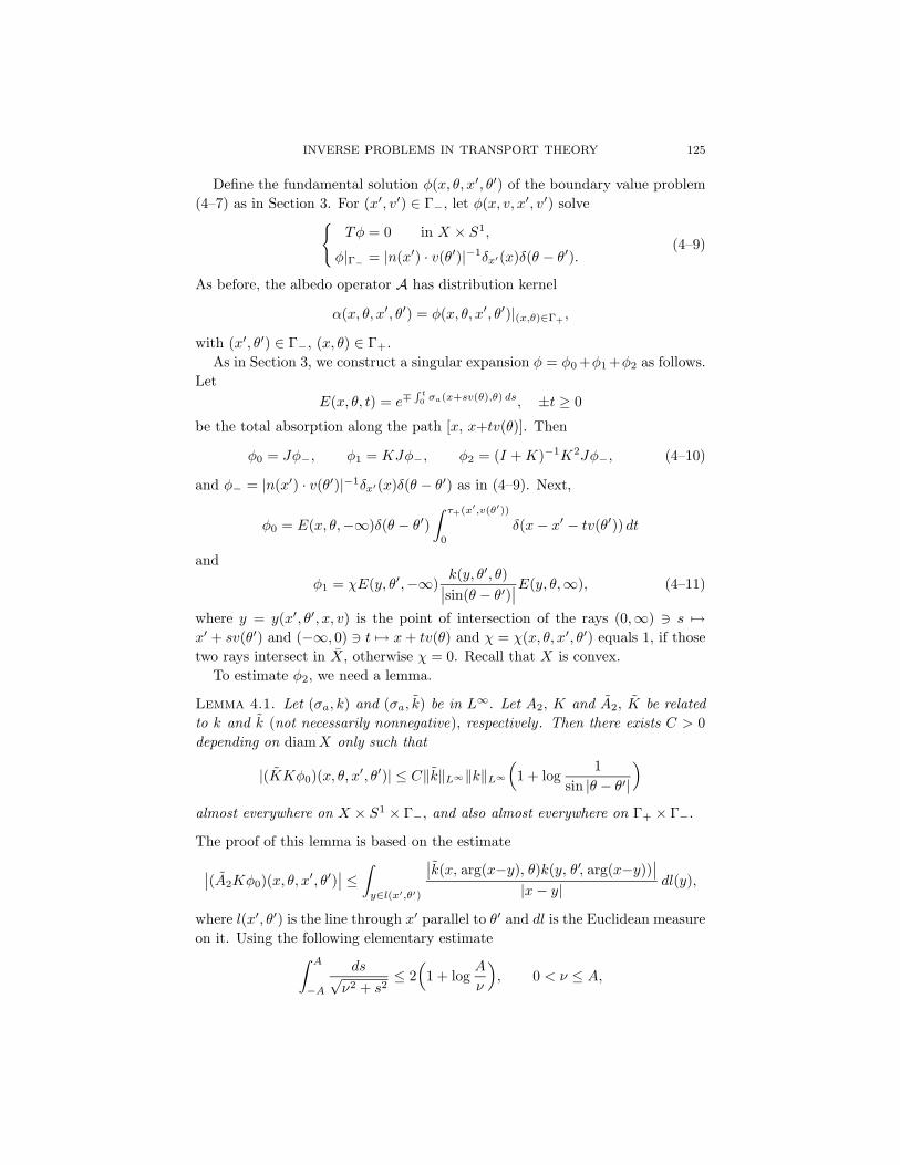
INVERSE PROBLEMS IN TRANSPORT THEORY 125
Define the fundamental solution φ(x, θ, x′, θ′) of the boundary value problem
(4–7) as in Section 3. For (x′, v′) ∈ Γ−, let φ(x, v, x′, v′) solve
Tφ = 0 in X × S1,
φ|Γ−= |n(x′) · v(θ′)|−1δx′(x)δ(θ − θ′).
(4–9)
As before, the albedo operator A has distribution kernel
α(x, θ, x′, θ′) = φ(x, θ, x′, θ′)|(x,θ)∈Γ+,
with (x′, θ′) ∈ Γ−, (x, θ) ∈ Γ+.
As in Section 3, we construct a singular expansion φ = φ0 +φ1 +φ2 as follows.
Let
E(x, θ, t) = e∓R
t
0σa(x+sv(θ),θ) ds, ±t ≥ 0
be the total absorption along the path [x, x+tv(θ)]. Then
φ0 = Jφ−, φ1 = KJφ−, φ2 = (I + K)−1K2Jφ−, (4–10)
and φ− = |n(x′) · v(θ′)|−1δx′(x)δ(θ − θ′) as in (4–9). Next,
φ0 = E(x, θ,−∞)δ(θ − θ′)
∫ τ+(x′,v(θ′))
0
δ(x − x′ − tv(θ′)) dt
and
φ1 = χE(y, θ′,−∞)k(y, θ′, θ)
∣
∣sin(θ − θ′)∣
∣
E(y, θ,∞), (4–11)
where y = y(x′, θ′, x, v) is the point of intersection of the rays (0,∞) 3 s 7→x′ + sv(θ′) and (−∞, 0) 3 t 7→ x + tv(θ) and χ = χ(x, θ, x′, θ′) equals 1, if those
two rays intersect in X, otherwise χ = 0. Recall that X is convex.
To estimate φ2, we need a lemma.
Lemma 4.1. Let (σa, k) and (σa, k) be in L∞. Let A2, K and A2, K be related
to k and k (not necessarily nonnegative), respectively . Then there exists C > 0
depending on diamX only such that
|(KKφ0)(x, θ, x′, θ′)| ≤ C‖k‖L∞‖k‖L∞
(
1 + log1
sin |θ − θ′|
)
almost everywhere on X × S1 × Γ−, and also almost everywhere on Γ+ × Γ−.
The proof of this lemma is based on the estimate
∣
∣(A2Kφ0)(x, θ, x′, θ′)∣
∣ ≤∫
y∈l(x′,θ′)
∣
∣k(x, arg(x−y), θ)k(y, θ′, arg(x−y))∣
∣
|x − y| dl(y),
where l(x′, θ′) is the line through x′ parallel to θ′ and dl is the Euclidean measure
on it. Using the following elementary estimate∫ A
−A
ds√ν2 + s2
≤ 2(
1 + logA
ν
)
, 0 < ν ≤ A,

126 PLAMEN STEFANOV
we easily complete the proof of the lemma.
For φ2 we therefore have φ2 = (I + K)−1φ#2 with φ#
2 = K2φ0 and by
Lemma 4.1,
0 ≤ φ#2 (x′, θ′, x, θ) ≤ C‖k‖2
L∞
(
1 + log1
∣
∣sin(θ − θ′)∣
∣
)
. (4–12)
This implies a similar estimate for φ2, because φ2 = φ#2 + (I − K)−1Kφ#
2 . We
summarize those estimates:
Proposition 4.1. For ε > 0 small enough, the fundamental solution φ of (4–7)
defined by (4–9) admits the representation φ = φ0 + φ1 + φ2 with
φ0 = E(x, θ,−∞)δ(θ − θ′)
∫ τ+(x′,v(θ′))
0
δ(x − x′ − tv(θ′)) dt,
φ1 = χE(y, θ′,−∞)k(y, θ′, θ)
| sin(θ − θ′)|E(y, θ,∞),
0 ≤ φ2 ≤ C‖k‖2L∞
(
1 + log1
∣
∣sin(θ − θ′)∣
∣
)
,
where y, χ are as in (4–11) and C = C(diamX).
Note that φ1 is not a delta function but it is still singular with singularity at
v(θ) = v(θ′) (forward scattering) and v(θ) = −v(θ′) (back-scattering). This
singularity is integrable however, in fact it is easy to see that∫
Γ+φ1dξ ≤
∫
σp(x′ + tv(θ′)) dt. The term φ2 is also singular at v(θ) = ±v(θ′) with a weaker,
logarithmic singularity. Therefore, we can still distinguish between the singular-
ities of the three terms as in the case n ≥ 3. This analysis however can give us
information about k only near forward and backward directions. It is interest-
ing to see whether by studying subsequent lower order terms we can recover all
derivatives of k(x, θ′, θ) at θ = θ′ and θ = θ′ + π. If so, this would allow us to
recover collision kernels analytic in θ, θ′ (actually, analytic in θ − θ′ would be
enough) and to approximate k near θ = θ′ and θ = θ′ + π for smooth k. This
would not require smallness assumptions on k but we still have to be sure that
the direct problem is solvable.
We are ready now to sketch the proof of Theorem 4.1. Fix Σ > 0 and assume
that we have two pairs (σa, k), (σa, k) in UΣ,ε with the same albedo operator and
σa, σa depending on x only. Denote by φj and φj , j = 0, 1, 2, the corresponding
components of the fundamental solutions φ and φ as in Proposition 4.1. Then
φ0 + φ1 + φ2 = φ0 + φ1 + φ2 for (x, θ) ∈ Γ+. (4–13)
As in Section 3, the most singular terms must agree; therefore,
φ0(x′, θ′, x, θ) = φ0(x
′, θ′, x, θ) for (x′, θ′) ∈ Γ−, (x, θ) ∈ Γ+. (4–14)
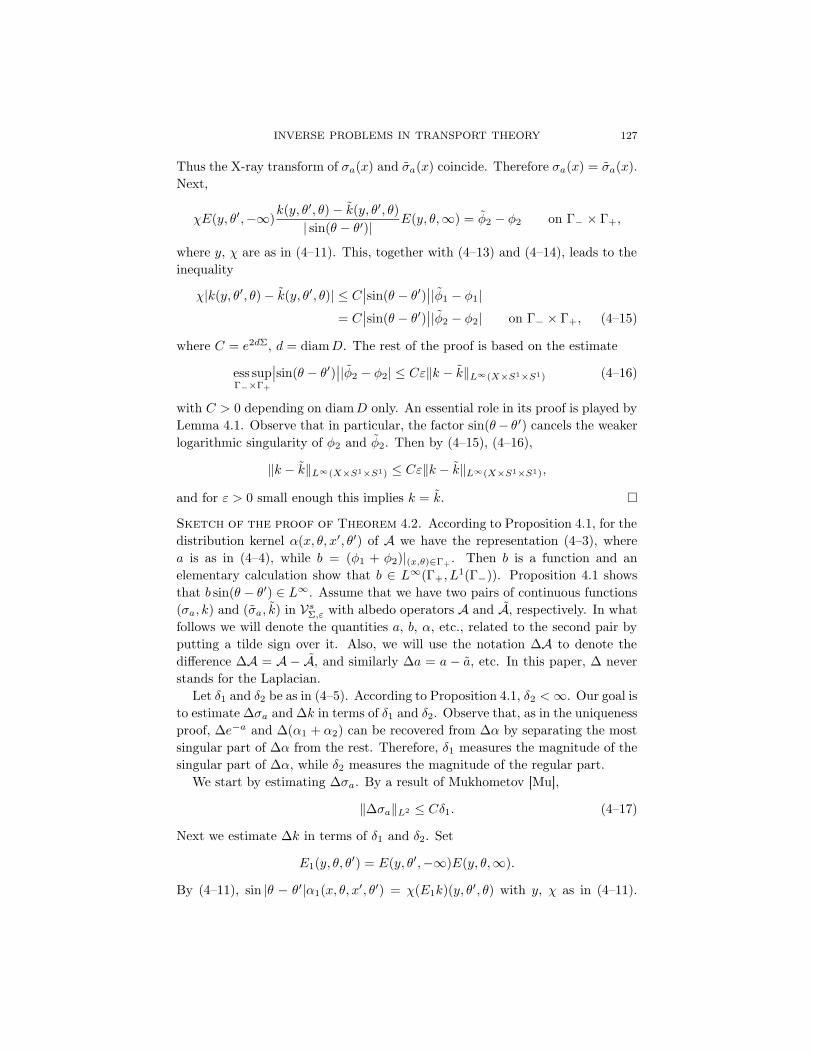
INVERSE PROBLEMS IN TRANSPORT THEORY 127
Thus the X-ray transform of σa(x) and σa(x) coincide. Therefore σa(x) = σa(x).
Next,
χE(y, θ′,−∞)k(y, θ′, θ) − k(y, θ′, θ)
| sin(θ − θ′)| E(y, θ,∞) = φ2 − φ2 on Γ− × Γ+,
where y, χ are as in (4–11). This, together with (4–13) and (4–14), leads to the
inequality
χ|k(y, θ′, θ) − k(y, θ′, θ)| ≤ C∣
∣sin(θ − θ′)∣
∣|φ1 − φ1|= C
∣
∣sin(θ − θ′)∣
∣|φ2 − φ2| on Γ− × Γ+, (4–15)
where C = e2dΣ, d = diamD. The rest of the proof is based on the estimate
ess supΓ−×Γ+
∣
∣sin(θ − θ′)∣
∣|φ2 − φ2| ≤ Cε‖k − k‖L∞(X×S1×S1) (4–16)
with C > 0 depending on diamD only. An essential role in its proof is played by
Lemma 4.1. Observe that in particular, the factor sin(θ− θ′) cancels the weaker
logarithmic singularity of φ2 and φ2. Then by (4–15), (4–16),
‖k − k‖L∞(X×S1×S1) ≤ Cε‖k − k‖L∞(X×S1×S1),
and for ε > 0 small enough this implies k = k. ˜
Sketch of the proof of Theorem 4.2. According to Proposition 4.1, for the
distribution kernel α(x, θ, x′, θ′) of A we have the representation (4–3), where
a is as in (4–4), while b = (φ1 + φ2)|(x,θ)∈Γ+. Then b is a function and an
elementary calculation show that b ∈ L∞(Γ+, L1(Γ−)). Proposition 4.1 shows
that b sin(θ − θ′) ∈ L∞. Assume that we have two pairs of continuous functions
(σa, k) and (σa, k) in VsΣ,ε with albedo operators A and A, respectively. In what
follows we will denote the quantities a, b, α, etc., related to the second pair by
putting a tilde sign over it. Also, we will use the notation ∆A to denote the
difference ∆A = A − A, and similarly ∆a = a − a, etc. In this paper, ∆ never
stands for the Laplacian.
Let δ1 and δ2 be as in (4–5). According to Proposition 4.1, δ2 < ∞. Our goal is
to estimate ∆σa and ∆k in terms of δ1 and δ2. Observe that, as in the uniqueness
proof, ∆e−a and ∆(α1 + α2) can be recovered from ∆α by separating the most
singular part of ∆α from the rest. Therefore, δ1 measures the magnitude of the
singular part of ∆α, while δ2 measures the magnitude of the regular part.
We start by estimating ∆σa. By a result of Mukhometov [Mu],
‖∆σa‖L2 ≤ Cδ1. (4–17)
Next we estimate ∆k in terms of δ1 and δ2. Set
E1(y, θ, θ′) = E(y, θ′,−∞)E(y, θ,∞).
By (4–11), sin |θ − θ′|α1(x, θ, x′, θ′) = χ(E1k)(y, θ′, θ) with y, χ as in (4–11).

128 PLAMEN STEFANOV
Our starting point is the relation ∆(E1k) = k∆E1 + E1∆k. Note first that
|∆E1| ≤ 2d|∆σa| ≤ 2dδ′1, where δ′1 = ‖∆σa‖L∞ . Hence, on supp χ,
E1|∆k|(y, θ, θ′) ≤ |∆(E1k)| + k|∆E1|≤ |∆(α1 + α2) sin |θ − θ′| − ∆α2 sin |θ − θ′|| + Cδ′1
≤ δ2 + |∆α2| sin |θ − θ′| + Cδ′1. (4–18)
Therefore,
‖∆k‖L∞ ≤ C(
δ′1 + δ2 + ‖∆α2 sin |θ − θ′|‖L∞
)
(4–19)
The next step is to prove an estimate similar to (4–16) for the last term in the
right-hand side above. Recall that in (4–16), we have σa = σa, while here we
only know how to estimate the difference ∆σa = σa − σa. Nevertheless, we can
proceed along similar lines in order to get
|∆α2 sin |θ − θ′|‖L∞ ≤ Cε(
‖∆k‖L∞ + δ′1)
. (4–20)
Therefore, for ε > 0 small enough, (4–19) implies the stability estimate
‖∆k‖L∞ ≤ C (δ′1 + δ2) . (4–21)
Estimate (4–21) is the base of our stability estimate. Using an interpolation
inequality, we conclude that, for any fixed 0 ≤ µ ≤ 1 − 1/s,
‖∆σa‖1+sµ ≤ C(Σ)‖∆σa‖1−1/s−µL2 for σa, σa ∈ Vs
Σ,ε.
By a standard Sobolev embedding theorem and (4–17),
δ′1 = ‖∆σa‖L∞ ≤ C(Σ)‖∆σa‖1−1/s−µL2 ≤ C ′(Σ)δ
1−1/s−µ1 . (4–22)
Therefore, (4–21) yields
‖∆k‖L∞ ≤ C(
δ1−1/s−µ1 + δ2
)
. (4–23)
Estimates (4–22) and (4–23) complete the proof of Theorem 4.2. ˜
5. Open Problems
Our choice of open problems is subjective and mainly reflects personal taste.
Uniqueness for σa depending on both x and v. As we have demonstrated
in the previous sections, if k = 0, then σa(x, v) cannot be recovered from A(or from the scattering operator) because the line integrals
∫
σa(x + tv, v) dt
do not recover σa. Suppose however that σp = σa. Then the absorption is
due only to the fact that particles may change velocity and each such event is
interpreted as a particle instantly moving from the point (x, v ′) of the phase
space (therefore absorption at (x, v′)) to the point (x, v). Then the counter
example above does not work. Can we recover σa(x, v) in this case? If yes, then
recovery of k goes along the same lines as above. More generally, one can assume

INVERSE PROBLEMS IN TRANSPORT THEORY 129
that σa(x, v) = σp(x, v)+a(x). Even more generally, the counter example above
cannot be generalized in an obvious way if k > 0 in X. Is this condition alone
enough for uniqueness?
Relaxing the smallness condition in the two-dimensional case. It would
be interesting to prove uniqueness in the 2D case without smallness assumption
on k. Some conditions on σa and k are needed even for the direct problem; see,
for example, (3–1) and (3–3) — the first one does require k to be small (but with
an explicit bound in general much larger than the one needed for the inverse
problem) while the second one does not. As mentioned in Section 4, one can try
to recover k(x, v′, v) near v = ±v′ at infinite order by studying the singularities
of the kernel of A which solves the problem for k analytic in v and v ′. It would
also be interesting to see whether one could recover the singularities of k from
boundary measurements, at least if we assume that they are of jump type across
some curve.
Stability for n ≥ 3. Stability estimates in dimensions n ≥ 3 have been proven
by Romanov (see [R1], [R2], [R3], for example) and by Wang [W], under addi-
tional assumptions that k depend on fewer variables. In the general situation
studied in Section 3, we know of no stability estimates, even for small k as in
Theorem 4.2 (where n = 2). We believe that such an estimate should be possi-
ble to derive following the proof of Theorem 3.1. This is done in [W] under the
additional assumption that k = k(v′, v).
Alternative recovery method for large σa and k. We do not impose small-
ness assumptions on the coefficients in dimensions n ≥ 3, and our method gives
in fact an explicit solution of the inverse problem which in particular implies a
reconstruction method based on taking certain limits near the singularity of α.
However, for large σa, the amplitude of the most singular part α0 is exponentially
small for large σa. For all practical purposes, measuring the leading singularity
is hard or impossible in this case. Therefore, it would be important to develop
a method for relatively large σa and k that does not rely on measuring the
singularities of α. One possible way is to study the diffusion limit (replacing σa
and k by λσa and λk and taking λ → ∞) and an associated inverse problem.
References
[AB] Yu. E. Anikonov, B. A. Bubnov, Inverse problems of transport theory, SovietMath. Doklady 37 (1988), 497–499.
[AE] P. Arianfar and H. Emamirad, Relation between scattering and albedo operators in
linear transport theory, Transport Theory and Stat. Physics, 23(4) (1994), 517–531.
[B] A. Bondarenko, The structure of the fundamental solution of the time-independent
transport equation, J. Math. Anal. Appl. 221:2 (1998), 430–451.
[Ce1] M. Cessenat, Théorèmes de trace Lp pour des espaces de fonctions de la neutron-
ique, C. R. Acad. Sci. Paris, Série I 299 (1984), 831–834.

130 PLAMEN STEFANOV
[Ce2] M. Cessenat, Théorèmes de trace pour des espaces de fonctions de la neutronique,C. R. Acad. Sci. Paris, Série I 300 (1985), 89–92.
[CMS] M. Chabi, M. Mokhtar-Kharroubi and P. Stefanov, Scattering theory with two
L1 spaces: application to transport equations with obstacles, Ann. Fac. Sci. Toulouse6(3) (1997), 511–523.
[CSt1] M. Choulli and P. Stefanov, Scattering inverse pour l’équation du transport et
relations entre les opérateurs de scattering et d’albédo, C. R. Acad. Sci. Paris 320
(1995), 947–952.
[CSt2] M. Choulli and P. Stefanov, Inverse scattering and inverse boundary value
problems for the linear Boltzmann equation, Comm. P.D.E. 21 (1996), 763–785.
[CSt3] M. Choulli and P. Stefanov, Reconstruction of the coefficients of the stationary
transport equation from boundary measurements, Inverse Prob. 12 (1996), L19–L23.
[CSt4] M. Choulli and P. Stefanov, An inverse boundary value problem for the station-
ary transport equation, Osaka J. Math. 36(1) (1999), 87–104.
[CZ] M. Choulli, A. Zeghal, Laplace transform approach for an inverse problem,Transport Theory and Stat. Phys., 24(9) (1995), 1353–1367.
[DL] R. Dautray and J.-L. Lions, Analyse Mathématique et Calcul Numérique pour les
Sciences et les Techniques, vol. 9, Masson, Paris, 1988.
[E] H. Emamirad, On the Lax and Phillips scattering theory for transport equation,J. Funct. Anal. 62 (1985), 276–303.
[EP] H. Emamirad and V.Protopopescu, Relationship between the albedo and scattering
operators for the Boltzmann equation with semi-transparent boundary conditions,Math. Meth. Appl. Sci., to appear.
[Hej] J. Hejtmanek, Scattering theory of the linear Boltzmann operator, Commun.Math. Physics 43 (1975), 109–120.
[H] S. Helgason, The Radon Transform, Birkhäuser, Boston, Basel, 1980.
[L1] E. W. Larsen, Solution of multidimensional inverse transport problems, J. Math.Phys. 25(1) (1984), 131–135.
[L2] E. Larsen, Solution of three-dimensional inverse transport problems, TransportTheory Statist. Phys. 17:2–3 (1988), 147–167.
[MC] N. J. McCormick, Recent developments in inverse scattering transport methods,Trans. Theory and Stat. Phys. 13 (1984), 15–28.
[Mo] M. Mokhtar-Kharroubi, Limiting absorption principle and wave operators on
L1(µ) spaces, Applications to Transport Theory, J. Funct. Anal. 115 (1993), 119-145.
[Mu] R. Mukhometov, On the problem of integral geometry, Math. Problems of
Geophysics, Akad. Nauk SSSR, Sibirs. Otdel., Vychisl. Tsentr, Novosibirsk, 6:2(1975), 212–242 (in Russian).
[PV] A. I. Prilepko, N. P. Volkov, Inverse problems for determining the parameters of
nonstationary kinetic transport equation from additional information on the traces
of the unknown function, Differentsialnye Uravneniya 24 (1988), 136–146.
[P1] V. Protopopescu, On the scattering matrix for the linear Boltzmann equation, Rev.Roum. Phys. 21 (1976), 991–994.
INVERSE PROBLEMS IN TRANSPORT THEORY 131
[P2] V. Protopopescu, Relation entre les opérateurs d’albédo et de Scattering avec des
conditions aux frontières non-transparentes, C. R. Acad. Sci. Paris, Série I 318
(1994), 83–86.
[RS] M. Reed and B. Simon, Methods of Modern Mathematical Physics, Vol. 3,Academic Press, New York, 1979.
[R1] V.G. Romanov, Estimation of stability in the problem of determining the attenua-
tion coefficient and the scattering indicatrix for the transport equation, Sibirsk. Mat.Zh. 37:2 (1996), 361–377, iii; translation in Siberian Math. J. 37:2 (1996), 308–324.
[R2] V.G. Romanov, Stability estimates in the three-dimensional inverse problem for
the transport equation, J. Inverse Ill-Posed Probl. 5:5 (1997), 463–475
[R3] V. Romanov, A stability theorem in the problem of the joint determination of
the attenuation coefficient and the scattering indicatrix for the stationary transport
equation, Mat. Tr. 1:1 (1998), 78–115.
[Si] B. Simon, Existence of the scattering matrix for linearized Boltzmann equation,Commun. Math. Physics 41 (1975), 99–108.
[St] P. Stefanov, Spectral and scattering theory for the linear Boltzmann equation, Math.Nachr. 137 (1988), 63–77.
[StU] P. Stefanov and G. Uhlmann, Optical Tomography in two dimensions, to appearin Methods Appl. Anal.
[SyU] J. Sylvester and G. Uhlmann, The Dirichlet to Neumann map and applications,in: Inverse Problems in Partial Differential Equations, SIAM Proceedings Series List(1990), 101–139, ed. by D. Colton, R. Ewing and R. Rundell.
[T] A. Tamasan, An inverse boundary value problem in two dimensional transport,Inverse Problems 18 (2002), 209-219.
[U] T. Umeda, Scattering and spectral theory for the linear Boltzmann operator,J. Math. Kyoto Univ. 24 (1984), 208–218.
[Vi] I. Vidav, Existence and uniqueness of non-negative eigenfunctions of the Boltz-
mann operator, J. Math. Anal. Appl. 22 (1968), 144-155.
[V1] J. Voigt, On the existence of the scattering operator for the linear Boltzmann
equation, J. Math. Anal. Appl. 58 (1977), 541–558.
[V2] J. Voigt, Spectral properties of the neutron transport equation, J. Math. Anal.Appl. 106 (1985), 140–153.
[W] J. Wang, Stability estimates of an inverse problem for the stationary transport
equation, Ann. Inst. H. Poincaré Phys. Théor. 70:5 (1999), 473–495.
Plamen Stefanov
Department of Mathematics
Purdue University
West Lafayette, IN 47907
United States