A Hamilton-Jacobi approach for a model of population structuredby space and trait

Emeric Bouin ∗ † Sepideh Mirrahimi ‡§

March 26, 2014

Abstract

We study a non-local parabolic Lotka-Volterra type equation describing a population struc-tured by a space variable x ∈ Rd and a phenotypical trait θ ∈ Θ. Considering diffusion, mu-tations and space-local competition between the individuals, we analyze the asymptotic (long–time/long–range in the x variable) exponential behavior of the solutions. Using some kind ofreal phase WKB ansatz, we prove that the propagation of the population in space can be de-scribed by a Hamilton-Jacobi equation with obstacle which is independent of θ. The effectiveHamiltonian is derived from an eigenvalue problem.The main difficulties are the lack of regularity estimates in the space variable, and the lack ofcomparison principle due to the non-local term.

Key-Words: Structured populations, Asymptotic analysis, Hamilton-Jacobi equation, Spectralproblem, Front propagationAMS Class. No: 45K05, 35B25, 49L25, 92D15, 35F21.

1 Introduction

It is known that the asymptotic (long-time/long-range) behavior of the solutions of some reaction-diffusion equations, as KPP type equations, can be described by level sets of solutions of somerelevant Hamilton-Jacobi equations (see [24, 22, 4, 8, 9, 31]). These equations, which admit trav-eling fronts as solutions, can be used as models in ecology to describe dynamics of a populationstructured by a space variable.A related, but different, method using Hamilton-Jacobi equations with constraint has been devel-oped recently to study populations structured by a phenotypical trait (see [19, 7, 29, 5, 27]). Thisapproach provides an asymptotic study of the solutions in the limit of small mutations and in longtime, and shows that the asymptotic solutions concentrate on one or several Dirac masses whichevolve in time.Is it possible to combine these two approaches to study populations structured at the same time bya phenotypical trait and a space variable?

∗Corresponding author†UMR CNRS 5669 ’UMPA’ and INRIA project ’NUMED’, École Normale Supérieure de Lyon, 46, allée d’Italie,

F-69364 Lyon Cedex 07, France. Email : emeric.bouin@ens-lyon.fr‡CNRS, Institut de Mathématiques de Toulouse UMR 5219, 31062 Toulouse, France. Email:

sepideh.mirrahimi@math.univ-toulouse.fr§Université de Toulouse ; UPS, INSA, UT1, UTM ; IMT ; 31062 Toulouse, France.

1

A challenge in evolutionary ecology is to provide and to analyze models that take into accountjointly the evolution and the spatial structure of a population. Most of the existing models whetherconcentrate on the evolution and neglect or simplify significantly the spatial structure, or deal onlywith the spatial dynamics of a population neglecting the impact of evolution on the dynamics. How-ever, to describe many phenomena in ecology, as the spatial structure and the local adaptation ofspecies [21], to understand the effect of environmental changes on a population [20] or to estimatethe propagation speed of an invasive species [30, 13], it is crucial to consider the interactions betweenecology and evolution. We refer also to [26] and the reference therein for general literature on thesubject.

In this paper, we study a population that is structured by a continuous phenotypical traitθ ∈ Θ, where Θ is a smooth and convex bounded subset of Rn, and a space variable x ∈ Rd. Theindividuals having a trait θ at time t and position x are denoted by n(t, x, θ). We assume that thepopulation moves (in space) with a diffusion process of diffusivity D > 0, and that they are subjectto mutations, which are also described by a diffusion term with diffusivity α > 0. We assume thatthe individuals in the same position are in competition with all other individuals, independently oftheir trait, and with a constant competition rate r. Let us notice that the non-locality in the modelcomes from here. We denote by ra(x, θ) ∈ C2

(Rd ×Θ

), the growth rate of trait θ at position x,

allowing, in this way, heterogeneity in space. The model reads∂tn = D∆xxn+ α∆θθn+ rn(a(x, θ)− ρ), (t, x, θ) ∈ (0,∞)× Rd ×Θ,

∂n

∂n= 0 on (0,∞)× Rd × ∂Θ,

n(0, x, θ) = n0(x, θ), (x, θ) ∈ Rd ×Θ.

(1.1)

We assume Neumann boundary conditions in the trait variable, meaning that the available traitsare given by the set Θ. Moreover, the initial condition n0 is given and nonnegative. The variable ρstands for the total density:

∀(t, x) ∈ R+ × Rd, ρ(t, x) =

∫Θn(t, x, θ)dθ.

Note that such equations can be derived from stochastic individual based models (see [16]).However, this is not the only way to couple the spatial and trait structures. One could also considera dependence in θ or x in the spatial diffusivity coefficient, the mutation rate or the competitionrate. See for instance [13] for a formal study of a model where the spatial diffusivity rate depends onthe trait but the growth rate is homogeneous in space. Although, there have been some attempts tostudy models structured by trait and space (see for instance [16, 2, 10, 13, 11]), not many rigorousstudies seem to have analyzed the dynamics of a population continuously structured by trait andby space, with non-local interactions. However, a very recent article [1], which studies a modelclose to (1.1) with some particular growth rate a(x, θ), proves existence of traveling wave solutions.Here, we consider a different approach where we perform an asymptotic analysis. Our objectiveis to generalize the methods developed recently on models structured only by a phenotypical trait[29, 5, 27] to spatial models, to be able to use the previous results in more general frameworks.Moreover, this approach allows us to study models with general growth rates a, where the speed ofpropagation is not necessarily constant. See also [28] for another work in this direction, where theHamilton-Jacobi approach is used to study a population model with a discrete spatial structure.

2

We expect that the population described by (1.1) propagates in the x-direction and that itattains a certain distribution in θ in the invaded parts. We seek for such behavior by performing anasymptotic analysis of the following rescaled model which corresponds to considering small diffusionin space and long time:

ε∂tnε = ε2D∆xxnε + α∆θθnε + rnε(a(x, θ)− ρε), (t, x, θ) ∈ (0,∞)× Rd ×Θ,

∂nε∂n

= 0 on (0,∞)× Rd × ∂Θ,

nε(0, x, θ) = n0ε(x, θ), (x, θ) ∈ Rd ×Θ.

(1.2)

We expect that, for ε small, nε can be approximated by

nε ≈ eu(t,x)ε Q(x, θ), with u(t, x) ≤ 0,

such that nε −−⇀ε→0

n, with

supp n ⊂ {(t, x)|u(t, x) = 0} ×Θ.

In this way, the propagation of the population would be described by the zero level sets of u. More-over, the phenotypical distribution of the population at position x would be given by Q(x, ·). Wewill show below that such approximation is possible with Q given by an eigenvalue problem and uthe unique solution to a Hamilton-Jacobi equation. These results allow us to derive the speed ofthe propagation and the phenotypical distribution of the population, in terms of the diffusion andmutation rates (D and α) and the fitness a(x, θ). Note that an important contribution in thesecomputations is the fact that both evolution processes and the movement of the individuals areconsidered jointly in the model. This is crucial to be able to understand several biological phenom-ena, as the spatial structure of Drosophila Subobscura, whose wing length increases clinally withlatitude [25] or the increasing speed of invasion of cane toads [30]. However, to be able to studyquantitatively the invasion of cane toads, one should also introduce a dependence in θ in the spatialdiffusion rate. This adds some technical difficulties that we leave for future work.

The purpose of this work is to derive rigorously the limit ε→ 0 in (1.2). Our study is based onthe usual Hopf-Cole transformation which is used in several works on reaction-diffusion equations(as for front propagation in [24, 22, 4]), in the study of parabolic integro-differential equationsmodeling populations structured by a phenotypical trait (see e.g. [19, 29]) and also recently in thestudy of the hyperbolic limit of some kinetic equations [12]:

uε := ε lnnε, or equivalently, nε = exp(uεε

). (1.3)

Thanks to standard maximum principle arguments, nε is nonnegative. The quantity uε is then welldefined for all ε > 0. By replacing (1.3) in (1.2) we obtain∂tuε = εD∆xxuε + α

ε∆θθuε +D|∇xuε|2 + αε2|∇θuε|2 + r(a(x, θ)− ρε), (t, x, θ) ∈ (0,∞)× Rd ×Θ,

∂uε∂n

= 0 on (0,∞)× Rd × ∂Θ,

uε(0, x, θ) = u0ε(x, θ) (x, θ) ∈ Rd ×Θ.

(1.4)

3

Throughout the paper, we will use the following assumptions:

∀ε > 0, ∀x ∈ Rd, −C1(x) ≤ u0ε ≤ C. (1.5)

limε→0

u0ε(x, θ) = u0(x), uniformly in θ ∈ Θ. (1.6)

∀(x, θ) ∈ Rd ×Θ, ψ(x) = −M |x|2 +B ≤ a(x, θ)− a∞ < 0, (1.7)

for some a∞ ∈ R. We also suppose the two following bounds:

‖∇θa(·, ·)‖∞ = b∞. (1.8)

∀x ∈ Rd, ρ0ε(x) ≤ a∞. (1.9)

To state our results we first need the following lemma:

Lemma 1. (Eigenvalue problem).For all x ∈ Rd, there exists a unique eigenvalue H(x) corresponding to a strictly positive eigen-

function Q(x, ·) ∈ C0(Θ) which satisfiesα∆2

θθQ+ ra(x, ·)Q = H(x)Q, in Θ,

∂Q(x, ·)∂n

= 0 on ∂Θ.(1.10)

The eigenfunction is unique under the additional normalization assumption

∀x ∈ Rd,∫

ΘQ(x, θ)dθ = 1. (1.11)

Moreover, H and Q are smooth functions.

We note that in this article, we suppose that Θ is bounded to avoid technical difficulties. How-ever, we expect that the results would remain true for unbounded domains Θ under suitable coer-civity conditions on −a such that the spectral problem (1.10) has a unique solution.

We can now state our main result:

Theorem 1. (Asymptotic behavior). Assume (1.5)–(1.9). Then

(i) The family (uε)ε converges locally uniformly to u : [0,∞) × Rd → R the unique viscositysolution of max(∂tu−D|∇xu|2 −H,u) = 0, in (0,∞)× Rd,

u(0, ·) = u0(·) in Rd.(1.12)

(ii) Uniformly on compact subsets of Int {u < 0} ×Θ, limε→0 nε = 0,

(iii) For every compact subset K of Int ({u(t, x) = 0} ∩ {H(x) > 0}), there exists C > 1 such that,

lim infε→0

ρε(t, x) ≥ H(x)

rC, uniformly in K. (1.13)

4

We notice that u does not depend on θ and therefore, we do not have any supplementary con-straint in (1.12) due to the boundary. The variational equality (1.12) gives indeed the effectivepropagation behavior of the population; the zero level-sets of u indicate where the population den-sity is asymptotically positive (see also Lemma 3). We recall that the effective Hamiltonian H in(1.12) is defined by the spectral problem (1.10) which hides the information on the trait variability.

To understand Theorem 1, it is illuminating to provide the following heuristic argument. Wewrite a formal expansion of uε:

uε(t, x, θ) = u0(t, x, θ) + εu1(t, x, θ) +O(ε2).

Replacing this in (1.4) and keeping the terms of order ε−2 we obtain, for all (t, x, θ),

|∇θu0(t, x, θ)|2 = 0.

This suggests that u0 should be independent of θ: u0(t, x, θ) = u0(t, x). Next, keeping the zeroorder terms (terms with coefficient ε0), yields:

−α(∆θu1 + |∇θu1|2

)− ra(x, θ) =

[−∂tu0 +D|∇xu0|2 − rρ0

](t, x). (1.14)

Here, ρ0 denotes the formal limit of ρε when ε → 0. Moreover, u1 satisfies Neumann boundaryconditions. Since the r.h.s. of (1.14) is independent of θ, Lemma 1 implies[

∂tu0 − |∇xu0|2 + rρ0

](t, x) = H(x) and u1(t, x, θ) = lnQ(x, θ) + µ(t, x).

We can now write

nε(t, x, θ) ≈ eu0(t,x)

ε+u1(t,x,θ), ρε(t, x) ≈ eµ(t,x)+

u0(t,x)ε .

As a consequence, ρε uniformly bounded implies that u0 is nonpositive. Furthermore

ρε > 0 =⇒ u0 = 0.

We deduce thatρ0(t, x) = 0 =⇒ ∂tu0(t, x)−D|∇xu0|2(t, x)−H(x) = 0,

ρ0(t, x) > 0 =⇒ u0(t, x) = 0 and r exp(µ(t, x)) = rρ0(t, x) = H(x),

and thusmax

(∂tu0 −D|∇xu0|2 −H(x) , u0

)= 0.

Moreover the above arguments suggest that

nε(t, x, θ) −→ε→0

H(x)r Q(x, θ) if u0(t, x) = 0,

0 if u0(t, x) < 0,

with Q and H given by Lemma 1. We notice finally that, the roles of the trait variable θ and thespectral problem (1.10) are respectively similar to the ones of the fast variable and the cell problemin homogenization theory.

5

Theorem 1 does not provide the limits of ρε and nε in Int ({u(t, x) = 0} ∩ {H(x) > 0}). Thedetermination of such limits in the general case, as was obtained for instance in [22], is beyond thescope of the present paper. The difficulty here is the lack of regularity estimates in the x-directionand the lack of comparison principle for the non-local equation (1.2). This difficulty also appears inthe study of propagating wave solutions of (1.1) (see [1]), where it is not clear whether the propagat-ing front is monotone and the density and the distribution of the population at the back of the frontis unknown. However, in Section 4 (see Proposition 2), we prove the convergence of nε and ρε ina particular case. The numerical results in Section 6.2 suggest that such limits might hold in general.

We emphasize that (1.2) does not admit a comparison principle which leads to technical diffi-culties. This is not only due to the presence of a non-local term but also due to the structure of thereaction term. We refer to [18, 14] for models admitting comparison principle although the reactionterms contain non-localities.

To prove the convergence of (uε)ε in Theorem 1, we use some regularity estimates that we statebelow.

Theorem 2. (Regularity results for uε). Assume (1.5), (1.7), (1.8), (1.9). Then the family(uε)ε>0 is uniformly locally bounded in R+×R×Θ. More precisely, the following inequalities hold:

∀(t, x, θ) ∈ R+ × Rd ×Θ, rψ(x)t− C1(x)− rεDMt2 ≤ uε(t, x, θ) ≤ C + ra∞t, (1.15)

where ψ(x) := −Mx2 + B. Next, let γ > 0 and for all ε > 0, vε :=√C + ra∞t+ γ2 − uε. Then,

for all ε > 0, the following bound holds:

∀(t, x, θ) ∈ R+ × Rd ×Θ, |∇θvε| ≤ε

2√αt

+

(rb∞ε

2

αγ

) 13

(1.16)

In particular, this gives a regularizing effect in trait for all t > 0, and the fact that ∇θvε convergeslocally uniformly to 0 when ε goes to 0.

We notice from (1.16) that, the limit of (vε)ε (and consequently the limit of (uε)ε) as ε→ 0, isindependent of θ for all t > 0, while we do not make any regularity assumption on the initial data.To obtain the regularizing effect in θ, we provide a Lipschitz estimate on a well-chosen auxiliaryfunction vε instead of uε, using the Bernstein method [17]. Note that, we do not have any estimateon the derivative of uε with respect to x due to the dependence of ρε on x. Therefore, we cannotprove the convergence of the uε’s as stated in Theorem 1 directly from the regularity estimatesabove. For this purpose, we use the so called half-relaxed limits method for viscosity solutions, see[6]. Moreover, to prove the convergence to the Hamilton-Jacobi equation (1.12) we are inspired fromthe method of perturbed test functions in homogenization [23].

Finally, the family (uε)ε being locally uniformly bounded from Theorem 2, we can introduce itsupper and lower semi-continuous envelopes that we will use through the article:

u(t, x, θ) := lim infε→0

(s,y,θ′)→(t,x,θ)

uε(s, y, θ′),

u(t, x, θ) := lim supε→0

(s,y,θ′)→(t,x,θ)

uε(s, y, θ′).

6

Thanks to Theorem 2, we know that |∇θuε| → 0 as ε → 0, for all t > 0. As a conclusion, theprevious limits do not depend on the variable θ. We have, for all θ ∈ Θ, x ∈ Rd and t > 0,

u(t, x, θ) = u(t, x) = lim infε→0

(s,y)→(t,x)

uε(s, y, θ), (1.17)

u(t, x, θ) = u(t, x) = lim supε→0

(s,y)→(t,x)

uε(s, y, θ), (1.18)

The remaining part of the article is organized as follows. Section 2 is devoted to the proofof Lemma 1 and Theorem 2. The convergence to the Hamilton-Jacobi equation (the first part ofTheorem 1) is proved in Section 3. In Section 4, using the Hamilton-Jacobi description, we studythe limits of nε and ρε and in particular complete the proof of Theorem 1. We also provide somequalitative properties on the effective Hamiltonian H and the corresponding eigenfunction Q inSection 5. Finally, in Section 6 we give some examples and comments on the spectral problem, andsome numerical illustrations for the time-dependent problem.

2 Regularity results (The proof of Theorem 2)

In this section we prove Theorem 2. To this end, we first provide a uniform upper bound on ρε (seeLemma 2). Next, using this estimate we give uniform upper and lower bounds on uε. Finally weprove a Lipschitz estimate with respect to θ on uε.

Lemma 2. (Bound on ρε).Assume (1.7) and (1.9). Then, for all ε > 0, the following a priori bound holds :

∀(t, x) ∈ R+ × Rd, 0 ≤ ρε(t, x) ≤ a∞. (2.19)

Proof of Lemma 2. The nonnegativity follows directly from the nonnegativity of nε. The upperbound can be derived using the maximum principle. We show indeed that ρε is a subsolution of asuitable Fisher-KPP equation. We integrate (1.2) in θ to obtain

ε∂tρε = ε2D∆xρε + r

(∫Θnε(t, x, θ)a(x, θ)dθ − ρ2

ε

).

Using (1.7) and the non negativity of nε, we deduce

ε∂tρε ≤ ε2D∆2xρε + rρε (a∞ − ρε) ,

so that the maximum principle and (1.9) ensure

∀(t, x) ∈ R+ × Rd, ρε(t, x) ≤ a∞.

We can now proceed with the proof of Theorem 2. For legibility, we divide the proof into severalsteps as follows.

7

# Step 1. Upper bound on uε. Define uε := uε − ra∞t. Using (1.4), we find

∂tuε = εD∆xuε +α

ε∆θuε +D|∇xuε|2 +

α

ε2|∇θuε|2 + r(a(x, θ)− a∞)− rρε.

Then, we conclude from (1.7), (1.5) and the maximum principle that

∀(t, x, θ) ∈ R+ × Rd ×Θ, uε(t, x, θ) ≤ u0ε(x, θ) + ra∞t ≤ C + ra∞t.

# Step 2. Lower bound on uε. From (1.4), (1.7) and Lemma 2 we can write

∂tuε ≥ εD∆xuε +α

ε∆θuε + r(a(x, θ)− a∞) ≥ εD∆xuε +

α

ε∆θuε + rψ(x),

with ψ(x) = −M |x|2 + B. Next we rewrite the above inequality, in terms of qε := uε − rψ(x)t +εrMDt2:

∂tqε ≥ εD∆xqε +α

ε∆θqε + rεψ′′(x)Dt+ 2rεMDt ≥ εD∆xqε +

α

ε∆θqε

Finally the maximum principle combined with Neumann boundary conditions and (1.5) imply that

uε ≥ u0ε + rψ(x)t− rεDMt2 ≥ −C1(x) + rψ(x)t− rεDMt2.

# Step 3. Lipschitz bound. We conclude the proof of Theorem 2 by using the Bernsteinmethod [17] to obtain a regularizing effect with respect to the variable θ. The upper bound (1.15)proved above ensures that the function vε is well-defined. We then rewrite (1.4) in terms of vε:

∂tvε = εD∆xvε+α

ε∆θvε+D

(ε

vε− 2vε

)|∇xvε|2 +

(α

εvε− 2αvε

ε2

)|∇θvε|2−

1

2vεr(a(x, θ)−a∞−ρε).

We differentiate the above equation with respect to θ and multiply it by ∇θvε|∇θvε| to obtain

∂t|∇θvε| ≤ εD∆x|∇θvε|+α

ε∆θ|∇θvε|+ 2D

(ε

vε− 2vε

)∇xvε · ∇x|∇θvε|

+ 2

(α

εvε− 2αvε

ε2

)∇θvε · ∇θ|∇θvε|+D

(− ε

v2ε

− 2

)|∇xvε|2|∇θvε|

+

(− α

εv2ε

− 2α

ε2

)|∇θvε|3 +

r|∇θa(x, θ)|2vε

, (2.20)

since the last contribution of the r.h.s of the above inequality becomes nonpositive. From (1.8) and(1.15), it follows that wε := |∇θvε| is a subsolution of the following equation

∂twε ≤ εD∆xw +α

ε∆θwε + 2D

(ε

vε− 2vε

)∇xvε · ∇xwε

+ 2

(α

εvε− 2αvε

ε2

)∇θvε · ∇θwε −

2α

ε2|wε|3 +

rb∞2γ

. (2.21)

The last step is now to prove that z(t) := ε2√αt

+(rb∞ε2

αγ

) 13 is a supersolution of (2.21). We compute

z′(t) +2α

ε2(z(t))3 =

2α

ε2

z(t)3 −

(z(t)−

(rb∞ε

2

αγ

) 13

)3 ≥ rb∞

2γ.

The Neumann boundary condition for uε implies a Dirichlet boundary condition for wε. Thus,(1.16) follows from the comparison principle.

8

3 Convergence to the Hamilton-Jacobi equation (The proof of The-orem 1–(i))

In this section, we first prove Lemma 1. Next, using the regularity estimates obtained above weprove the convergence of (uε)ε to the solution of (1.12) (Theorem 1 (i)). This will be derived fromthe following proposition which also provides a partial result, once we relax assumption (1.6):

Proposition 1. (Convergence to the Hamilton-Jacobi equation).

(i) Assume (1.5), (1.7), (1.8), (1.9) such that Theorem 2 holds. Let H be the eigenvalue definedin Lemma 1. Then, u (respectively u) is a viscosity subsolution (respectively supersolution) of

max(∂tu−D|∇xu|2 −H,u) = 0, in (0,∞)× Rd. (3.22)

(ii) If we assume additionally (1.6), then u = u and, as ε vanishes, (uε)ε converges locally uni-formly to u = u = u the unique viscosity solution ofmax(∂tu−D|∇xu|2 −H,u) = 0, in (0,∞)× Rd,

u(0, x) = u0(x).

Before proving Proposition 1, we first give a short proof for Lemma 1.

Proof of Lemma 1. Let X = C1,µ (Θ) and K be the positive cone of nonnegative functions in X.We define L : X → X as below

L(u) = −α∆θθu− r (a(x, θ)− a∞)u.

The resolvent of L together with the Neumann boundary condition is compact from the regularizingeffect of the Laplace term. Moreover, the strong maximum principle gives that it is also stronglypositive. Using the Krein-Rutman theorem we obtain that there exists a nonnegative eigenvaluecorresponding to a positive eigenfunction. This eigenvalue is simple and none of the other eigenvaluescorrespond to a positive eigenfunction. This defines H(x) and Q(x, θ) in (1.10) in a unique way.The smoothness of H and Q derives from the smoothness of a(x, θ) and the fact that they areprincipal eigenelements.

Proof of Proposition 1. We prove the result in two steps.

a. Discontinuous stability (proof of (i)).

To prove the result we need to show that u and u are respectively sub and supersolutions of (3.22).

a.1. We prove that u ≤ 0.

Suppose that there exists a point (t, x) such that u(t, x) > 0. From (1.18) and (1.16), thereexists a sequence εn → 0 and a sequence of points (tn, xn) →

n→∞(t, x) such that,

uεn(tn, xn, θ) →n→∞

u(t, x), uniformly in θ.

9

As a consequence, there exists δ > 0 such that for n sufficiently large, uεn(tn, xn, θ) > δ, for allθ ∈ Θ. This implies

ρεn(tn, xn) =

∫Θ

exp

(uεn(tn, xn, θ)

εn

)dθ ≥ |Θ| exp

(δ

εn

)> a∞,

for sufficiently large n, which is in contradiction with Lemma 2.

a.2. We prove that ∂tu−D|∇xu|2 −H ≤ 0.

Now, assume that ϕ ∈ C2 (R+ × R) is a test function such that u(t, x)−ϕ(t, x) has a strict localmaximum at (t0, x0).

Using the eigenfunction Q introduced in Lemma 1, we can define a corrected test function[23] by χε = ϕ(t, x) + εη(x, θ), with η(x, θ) = ln (Q (x, θ)). Using standard arguments in thetheory of viscosity solutions (see [3]), there exists a sequence (tε, xε, θε) such that the functionuε(t, x, θ) − χε(t, x, θ) takes a local maximum in (tε, xε, θε), which is strict in the (t, x) variables,and such that (tε, xε) → (t0, x0) as ε → 0. Moreover, as θε lies in the compact set Θ, one canextract a converging subsequence. For legibility, we omit the extraction in the sequel.

Let us verify the viscosity subsolution criterion. At the point (tε, xε, θε), we have:

∂tχε −D|∇xχε|2 −H(xε) = ∂tuε −D|∇xuε|2 −H(xε),

= εD∆xuε + αε∆θuε + α

ε2|∇θuε|2 + r(a(xε, θ)− ρε)−H(xε),

≤ εD∆xχε + αε∆θχε + α

ε2|∇θχε|2 + ra(xε, θ)−H(xε).

We must emphasize that the Neumann boundary conditions are implicitly used here in case whenθε is on the boundary of Θ. Indeed, this ensures that we have ∇θχε(tε, xε, θε) = 0 in this latter case.As a consequence, we still have ∇θuε(tε, xε, θε) = ∇θχε(tε, xε, θε) so that the first order derivative inthe trait variable does not add any supplementary difficulty in the r.h.s.. Moreover the second orderterms still have the right sign, since again ∆2

xxuε ≤ ∆2xxχε is enforced by the Neumann boundary

condition.

We replace the test function by its definition to obtain

∂tϕ−D|∇x (ϕ+ εη) |2−H(xε) ≤ εD(∆2xxϕ+ ε∆xxη

)+α

(∆2θθη + |∇θη|2

)+ra(xε, θ)−H(xε).

Here appears the crucial importance of choosing η = lnQ with Q the solution of the spectralproblem (1.10). Coupling the above equation with the spectral problem (1.10), written in terms ofη, we deduce that

∂tϕ−D|∇xϕ+ εη|2 −H(xε) ≤ εD(∆2xxϕ+ ε∆xxη

).

We conclude, by letting ε go to 0, that at point (t0, x0):

∂tϕ−D|∇xϕ|2 −H ≤ 0.

a.3. We prove that max(∂tu−D|∇xu|2 −H,u

)≥ 0.

10

We first notice that u(t, x) ≤ u(t, x) ≤ 0. Let u(t, x) < 0. Then there exists some δ > 0 suchthat along a subsequence (εn, tn, xn), uεn(tn, xn, θ) < −δ for all θ ∈ Θ and for n ≥ N with Nsufficiently large. It follows that ρεn(tn, xn) → 0, as n → ∞. With the same notations as in theprevious point replacing maximum by minimum, we get

∂tϕ−D|∇xϕ+ εη|2 −H(xε) ≥ εD(∆2xxϕ+ ε∆xxη

)− rρε,

so that taking the limit ε→ 0 along the subsequence (tεn , xεn), we obtain that

∂tϕ−D|∇xϕ|2 −H ≥ 0.

holds at point (t0, x0).

b. Strong uniqueness (proof of (ii)).

Obviously, one cannot get any uniqueness result for the Hamilton-Jacobi equation (3.22) withoutimposing any initial condition. Adding (1.6), we now check the initial condition of (1.12) in theviscosity sense.

One has to prove the following

min(max

(∂tu−D|∇xu|2 −H,u

), u− u0

)≤ 0, in {t = 0} × Rd, (3.23)

andmax

(max

(∂tu−D|∇xu|2 −H,u

), u− u0

)≥ 0, in {t = 0} × Rd, (3.24)

in the viscosity sense.Here we give only the proof of (3.23), since (3.24) can be derived following similar arguments.

Let ϕ ∈ C2 (R+ × R) be a test function such that u(t, x) − ϕ(t, x) has a strict local maximum at(t0 = 0, x0). We now prove that either

u(0, x0) ≤ u0(x0),

or ∂tϕ(0, x0)−D|∇xϕ(0, x0)|2 −H(x0) ≤ 0,

and

u(0, x0) ≤ 0.

Suppose then thatu(0, x0) > u0(x0). (3.25)

Following the arguments above in a.1. but taking t = 0 and using (1.6) we obtain

u(0, x0) ≤ 0.

We next prove that∂tϕ(0, x0)−D|∇xϕ(0, x0)|2 −H(x0) ≤ 0. (3.26)

There exists a sequence (tε, xε, θε)ε such that (tε, xε) tends to (0, x0) as ε→ 0 and that uε − χε =uε − ϕ − εη takes a local maximum at (tε, xε, θε). Here η still denotes the correction lnQ with Qthe eigenfunction introduced in Lemma 1 (see a.1.). We first claim that there exists a subsequence

11

(tn, xn, θn)n of the above sequence and a subsequence (εn)n, with εn → 0 as n → ∞, such thattn > 0, for all n.

Suppose that this is not true. Then, there exists a sequence (εn′ , xn′ , θn′)n′ such that (εn′ , xn′)→(0, x0) and that uεn′ − ϕ− εn′η has a local maximum at (0, xn′ , θn′). It follows that, for all (t, x, θ)in some neighborhood of (0, xn′ , θn′), we have

uεn′ (0, xn′ , θn′)− χεn′ (0, xn′ , θn′) ≥ uεn′ (t, x, θ)− χεn′ (t, x, θ) .

Computing lim supn′→∞

(t,x)→(t0,x0)

at the both sides of the inequality, and using (1.6) one obtains

u0 (x0)− ϕ (0, x0) ≥ u (0, x0)− ϕ (0, x0) .

However, this is in contradiction with (3.25). We thus proved the existence of subsequences(tn, xn, θn)n and (εn)n described above with tn > 0, for all n.

Now having in hand that tn > 0, from (1.4) and the fact that uεn − ϕ − εnη takes a localmaximum at (tn, xn, θn), we deduce that

∂tϕ−D|∇xϕ+ εnη|2 −H(xεn) ≤ εnD(∆2xxϕ+ εn∆xxη

)holds in (tn, xn, θn). Finally, letting n→ +∞, we find (3.26).

We refer to [3, Section 4.4.5] and [22, Theorem B.1] for arguments giving strong uniqueness(i.e. a comparison principle for semi-continuous sub and supersolutions) for (1.12). As u and uare respectively sub and supersolutions of (1.12), we then know that u ≤ u. From their earlydefinition, we also have u ≥ u. Gathering these inequalities, we finally obtain u = u = u and that(uε)ε converges locally uniformly, as ε → 0, towards u, the unique viscosity solution of (1.12) inR+ × Rd ×Θ.

4 Refined asymptotics (The proof of Theorem 1–(ii) and (iii))

In this section, we provide some information on the asymptotic population density. Firstly, we proveparts (ii) and (iii) of Theorem 1 which state that the zero sets of u correspond to the zones wherethe population is positive. Secondly, we provide the limit of (nε)ε, as ε → 0, in a particular case(see Proposition 2).

We first prove the following lemma:

Lemma 3. Let u be the unique viscosity solution of (1.12) and H(x) the eigenvalue given by Lemma1. Then

(t, x) ∈ Int {u(t, x) = 0} =⇒ H(x) ≥ 0.

Proof of Lemma 3. Thanks to (1.12),

∂tu−D|∇xu|2 ≤ H(x),

12

in the viscosity sense. In the zone Int {u(t, x) = 0}, one has

∂tu−D|∇xu|2 = 0,

in the strong sense. The proof of the lemma follows.

We now are able to characterize the different zones of the front and complete the proof ofTheorem 1:

Proof of Theorem 1, (ii). Let K be a compact subset of Int {u < 0}. The local uniform conver-gence of uε towards u ensures that there exists a constant δ > 0 such that for sufficiently small ε > 0and for all (t, x) ∈ K and θ ∈ Θ, uε(t, x, θ) < −δ. As a consequence, nε = exp

(uεε

)< exp

(− δε

)→ 0,

uniformly as ε→ 0 in K ×Θ.

Proof of Theorem 1, (iii). Take (t0, x0) ∈ K ⊂⊂ Int ({u = 0} ∩ {H(x) > 0}), and let Q be thenormalized eigenvector given by Lemma 1. We denote Cm = Cm(x0) = minΘQ(x0, θ) and CM =CM (x0) = maxΘQ(x0, θ). We also define

Fε(t, x) :=

∫Θnε(t, x, θ)Q(x0, θ)dθ, Iε := ε lnFε.

Using classical arguments, one can prove that I := limε→0 Iε is well-defined and nonpositive. Wealso point out that {u = 0} = {I = 0} since

minθuε(t, x, θ) + o(1) ≤ Iε(t, x) ≤ max

θuε(t, x, θ) + o(1),

for all (t, x) ∈ [0,∞)× Rd. Multiplying equation (1.2) by Q(x0, θ) and integrating in θ yields

ε∂tFε − ε2D∆xFε − α∫

Θnε∆θQ(x0, θ) = r

∫Θa(x, θ)Q(x0, θ)nε(t, x, θ)dθ − rρεFε.

Combining the above equation by (1.10) we deduce that

ε∂tFε − ε2D∆xFε = (H(x0)− rρε)Fε + r

∫ΘQ(x0, θ)nε(t, x, θ) [a(x, θ)− a(x0, θ)] dθ.

Since H(x0) > 0 and a is continuous, for all δ > 0, one can choose a constant r > 0 such that

∀x ∈ Br(x0), |a(x, θ)− a(x0, θ)| < δH(x0) with Br(x0) ⊂ K.

We finally deduce that for all x ∈ Br(x0),

ε∂tFε − ε2D∆xFε ≥ ((1− δ)H(x0)− rρε)Fε.

Since Fε ≥ Cmρε, it follows that for all x ∈ Br(x0),

ε∂tFε − ε2D∆xFε ≥(

(1− δ)H(x0)− rFεCm

)Fε. (4.27)

Moreover, since (t0, x0) ⊂ Int{u(t, x) = 0} = Int{I(t, x) = 0}, we have I(t, x) = 0 in a neighborhoodof (t0, x0).

13

We then apply an argument similar to the one used in [22] to prove an analogous statement forthe Fisher-KPP equation. To this end, we introduce the following test function

ϕ(t, x) = −|x− x0|2 − (t− t0)2.

As I − ϕ attains a strict minimum in (t0, x0), there exists a sequence (tε, xε) of points such thatand Iε − ϕ attains a minimum in (tε, xε), with (tε, xε)→ (t0, x0). It follows that

∂tϕ− εD∆xϕ−D|∇xϕ|2 ≥ ∂tIε − εD∆xIε −D|∇xIε|2 = (1− δ)H(x0)− rFεCm

.

As a consequence,

lim infε→0

Fε(t0, x0) ≥ Cmr

(1− δ)H(x0),

uniformly with respect to points (t0, x0) ∈ K and this gives

lim infε→0

ρε(t0, x0) ≥ (1− δ)H(x0)CmrCM

.

We then let δ → 0 and obtain

lim infε→0

ρε(t0, x0) ≥ H(x0)Cm(x0)

rCM (x0),

uniformly with respect to points (t0, x0) ∈ K.

LetK = {x | ∃t ≥ 0, such that (t, x) ∈ K}.

To conclude the proof, it is enough to prove that there exists a constant C = C(α, r, a|K×Θ

) ≥ 1,such that

CM (x)

Cm(x)≤ C, for all x ∈ K.

This is indeed a consequence of the Harnack inequality [15] for the solutions of (1.10) in Θ for allx ∈ K. We point out that here we can use the Harnack inequality on the whole domain Θ thanksto the Neumann boundary condition.

The above result is not enough to identify the limit of (nε)ε as ε → 0, as was obtained forexample for Fisher-KPP type models in [22]. The main difficulties to obtain such limits are thefacts that we do not have any regularity estimate in the x direction on nε and that there is nocomparison principle for this model due to the non-local term. However, we were able to identifythe limit of (nε)ε in a particular case:

Proposition 2. Suppose that Q, the eigenvector given by (1.10), does not depend on x, i.e.Q(x, θ) = Q(θ). Let the initial data be of the following form

nε(t = 0, x, θ) = mε(x)Q(θ), mε(x) ≥ 0. (4.28)

Then:

(i) For all t > 0 and (x, θ) ∈ Rd ×Θ, nε(t, x, θ) = mε(t, x)Q(θ).

14

(ii) For all (t, x, θ) ∈ {u(t, x) = 0} ×Θ, limε→0 nε(t, x, θ) = H(x)r Q(θ).

Remark 1. We note that the assumption on Q in Proposition 2, is satisfied for a(x, θ) = a(θ)+b(x).

Proof of Proposition 2. Let mε be the unique solution of the following equation{ε∂tmε − ε2D∆xmε = rmε (H(x)−mε) ,

mε(0, x) = mε(x).

Definenε(t, x, θ) := mε(t, x)Q(θ).

We notice from (1.11) that ∫nε(t, x, θ)dθ = mε(t, x).

Consequently, from (4.28), (1.10), and the definition of mε one can easily verify that nε is a solutionof (1.2), and since (1.2) has a unique solution we conclude that

nε(t, x, θ) = mε(t, x)Q(θ),

andρε(t, x) = mε(t, x).

As a consequence ρε satisfies the following Fisher-KPP equation

ε∂tρε − ε2D∆xρε = rρε (H(x)− ρε) .

Let (t, x) ∈ {u = 0}. Then from Lemma 3, we obtain H(x) ≥ 0. Hence, from the above equationand (1.13), following similar arguments as in [22] (page 157) we obtain that ρε(t, x) → H(x) asε→ 0, and (ii) follows.

5 Qualitative properties

In this section, we provide some estimates on the effective Hamiltonian H and the eigenfunction Q.We note that the spatial propagation of the population can be described using H through (1.12).In particular, if H(x) = H is constant and if initially the population is restricted to a compact setin space, then the population propagates in space with the constant speed c = 2

√H. Furthermore,

the eigenfunction Q is expected to represent the phenotypical distribution of the population (seeProposition 2).

We begin by presenting some qualitative estimates on the effective Hamiltonian H.

Lemma 4. The eigenvalue and normalized eigenfunction introduced in Lemma 1 satisfy the followingestimates:

∀x ∈ R, H(x) = r

∫Θa(x, θ)Q(x, θ)dθ, (5.29)

∀x ∈ R,r

Θ

∫Θa(x, θ)dθ ≤ H(x) ≤ ra(x, θ(x)) (5.30)

where θ is a trait which maximizes Q(x, ·): Q(x, θ(x)) = maxΘQ(x, θ).

15

In particular, the eigenvalue H(x), which more or less represents the speed of the front, is notnecessarily given by the most privileged individuals, that is those having the largest fitness a. SeeExample 4 for a case where the inequality is strict. This property confirms that the front may slowdown due to very unfavorable traits.

Proof of Lemma 4. By integrating (1.10) with respect to θ and using the Neumann boundarycondition and (1.11), we find (5.29).

To prove (5.30) we rewrite (1.10) in terms of η = lnQ:

∀(x, θ) ∈ R×Θ, H(x) = α(∆θθη + |∇θη|2

)+ ra(x, θ) (5.31)

Then, integrating and using the Neumann boundary conditions in the variable θ for η, one obtains

H(x) ≥ r

|Θ|

∫Θa(x, θ)dθ.

Let Q(x, θ(x)) = maxΘQ(x, θ). Then ∇θη(x, θ(x)) = 0 and ∆θη(x, θ(x)) ≤ 0. Evaluating (5.31) inθ(x), we get

H(x) ≤ ra(x, θ(x)).

Lemma 5. Let a(x, ·) be a strictly concave function on Θ := [θm, θM ] for all x ∈ R. Then for allx ∈ R, the maximum of Q(x, ·) is attained in only one point θ(x).

Proof of Lemma 5. The concavity hypothesis implies that for all x ∈ R, the function H(x) −ra(x, ·) is strictly convex. Thus, on the interval [θm, θM ], it has at most two zeros. The case of nozeros is excluded from (5.30). Let’s study the two remaining cases.

Suppose it has only one zero at θ (see Example 1), say it is positive on[θm, θ

[and nonpositive

on[θ, θM

[. Then from the early definition of the spectral problem, Q(x, ·) is convex on

[θm, θ

[and

concave on[θ, θM

[. The Neumann boundary conditions enforce that Q(x, ·) is increasing on Θ, and

attains its maximum at θ = θM .Suppose it has two zeroes, at θ1 and θ2. Then H(x) − ra(x, ·) is nonnegative on

[θm, θ1

[and[

θ2, θM

[, and negative on

[θ1, θ2

[. As a consequence, by the same convexity analysis as in the

previous case, Q(x, ·) attains its maximum on[θ1, θ2

[, where it is strictly concave, which justifies

the existence and uniqueness of θ.

Remark 2. (Limit as α→ 0).As the mutation rate α goes to 0, we expect that the eigenfunction Qα converges towards a sum

of Dirac masses. To justify this, we use again a WKB ansatz, setting ϕα =√α ln (Qα). Rewriting

(1.10) in terms of ϕα we obtain√α∆θϕα + |∇θϕα|2 + ra(x, θ)−Hα(x) = 0.

16

It is classical that the family ϕα is equi-Lipschitz and we can extract a subsequence that convergesuniformly. We have indeed that as α→ 0, (ϕα, Hα) converges to (ϕ,H), with ϕ a viscosity solutionof the following equation |∇θϕ|

2 + ra(x, θ)−H(x) = 0,

H(x) = maxθ∈Θ ra(x, θ).

Moreover from (1.11) we obtain that

maxθ∈Θ

ϕ(x, θ) = 0.

Finally, we conclude from the above equations that as α→ 0, Qα−−⇀ Q with Q a measure satisfying

supp Q(x, ·) ⊂ {θ ∈ Θ |ϕ(x, θ) = 0} ⊂ {θ ∈ Θ |H(x) = ra(x, θ) = rmaxθ∈Θ

a(x, θ)}.

In other terms, in the limit of rare mutations, the population concentrates on the maximum pointsof the fitness a(x, θ).

6 Examples and numerics

6.1 Examples of spectral problems

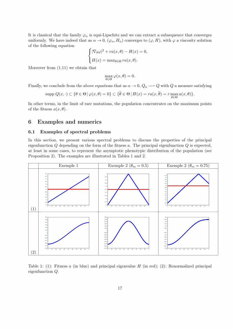
In this section, we present various spectral problems to discuss the properties of the principaleigenfunction Q depending on the form of the fitness a. The principal eigenfunction Q is expected,at least in some cases, to represent the asymptotic phenotypic distribution of the population (seeProposition 2). The examples are illustrated in Tables 1 and 2.

Exemple 1 Exemple 2 (θm = 0.5) Exemple 2 (θm = 0.75)

(1)

(2)

Table 1: (1): Fitness a (in blue) and principal eigenvalue H (in red); (2): Renormalized principaleigenfunction Q.

17

Example 1. (A fitness with linear dependence on θ).This example is taken from [13]. For θ ∈ [θm, θM ] and b : R → Θ a smooth function, let

a(x, θ) = µθ − b(x). The spectral problem writes, for all x ∈ R:α∂θθQ+ rθQ = (H(x) + rb(x))Q,

∂θQ(x, θm) = ∂θQ(x, θM ) = 0.

The solution of this problem is unique up to a multiplicative constant and can be expressedimplicitly with special Airy functions. In Table 1, for α = 1, r = 2 and Θ = [0, 1], we plot thefitness a(θ) = θ

2 + 14 and the associated eigenvector Q. Beware that this example will be used again

in Section 6.2.

Example 2. (The maxima of a and Q are not always at the same points.)For Example 2, we consider a(x, θ) := 1− |θ − θm|, for different values of θm ∈ Θ := [0, 1]. The

parameters for the simulations are α = 1, r = 1. We observe that although the fitness a attainsits maximum at θ = θm, it is not given that the maximum of the eigenfunction Q is attained atθ = θm. In other words, the trait with the optimal fitness value does not necessarily correspond tothe most represented one. Indeed, when θm = 1

2 , the eigenfunction Q is necessarily symmetric withrespect to θm = 1

2 , and hence attains a maximum at this point. By contrast, for θm = 34 , the most

represented trait is not the most favorable one (see Table 1): The diffusion through the Neumannboundary condition plays a strong role in this case. We observe indeed with this example that,while the fitness a has a non-symmetric profile, the maximum points of Q can be far from the onesof a, due to the diffusion term. However, while α (which equals 1 in this example) takes values closeto 0, the maximum points of Q approach the ones of a.

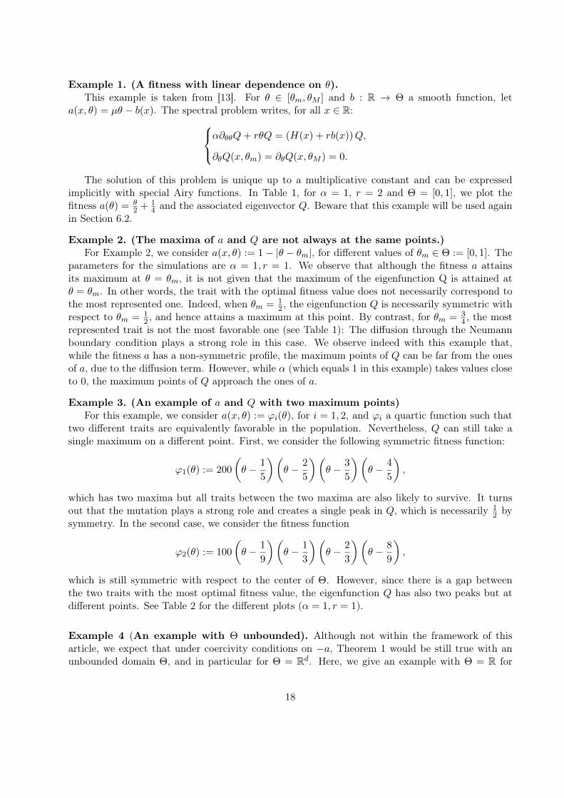
Example 3. (An example of a and Q with two maximum points)For this example, we consider a(x, θ) := ϕi(θ), for i = 1, 2, and ϕi a quartic function such that

two different traits are equivalently favorable in the population. Nevertheless, Q can still take asingle maximum on a different point. First, we consider the following symmetric fitness function:

ϕ1(θ) := 200

(θ − 1

5

)(θ − 2

5

)(θ − 3

5

)(θ − 4

5

),

which has two maxima but all traits between the two maxima are also likely to survive. It turnsout that the mutation plays a strong role and creates a single peak in Q, which is necessarily 1

2 bysymmetry. In the second case, we consider the fitness function

ϕ2(θ) := 100

(θ − 1

9

)(θ − 1

3

)(θ − 2

3

)(θ − 8

9

),

which is still symmetric with respect to the center of Θ. However, since there is a gap betweenthe two traits with the most optimal fitness value, the eigenfunction Q has also two peaks but atdifferent points. See Table 2 for the different plots (α = 1, r = 1).

Example 4 (An example with Θ unbounded). Although not within the framework of thisarticle, we expect that under coercivity conditions on −a, Theorem 1 would be still true with anunbounded domain Θ, and in particular for Θ = Rd. Here, we give an example with Θ = R for

18

Exemple 3 (ϕ1) Exemple 3 (ϕ2)

(1)

(2)

Table 2: Fitness a (in blue) and principal eigenvalue H (in red); (2): Renormalized principaleigenfunction Q.

which it is easy to compute the eigenelements Q and H. We consider a (x, θ) := a∞− b∞2 (θ − b(x))2

where b : R→ R is a smooth function. We can then compute:

Q(x, θ) = exp

(−1

2

√rb∞2α

(θ − b(x))2

), H(x) = H = ra∞ −

√rαb∞

2.

This suggests that, the most represented trait at position x is given by θ = b(x), and the speed ofthe propagation of the population is 2

√H.

These solutions are not valid in a bounded domain since they do not satisfy the Neumann bound-ary conditions.

We note that, with these parameters, the left inequality in (5.30) is strict, i.e. H(x) <ra(x, θ(x)) = ra∞, but as b∞ → 0, which corresponds to the limit case where all the traits areequally favorable, we have H(x)→ ra∞. Finally, it is interesting to notice here that to ensure frontexpansion, i.e. H(x) ≥ 0, the fitness must satisfy the following additional condition 2a2∞

b∞≥ α

r .

6.2 Numerical illustrations on the evolution of the front

In this section, we resolve numerically the evolution problem (1.2) for three different values of a.For all the examples, we choose the following initial data{

nε(0, x, θ) = max(

1, 2− 8(θ − 1

2

)2) if x ∈ [0, 0.5], θ ∈ Θ := [0, 1],

nε(0, x, θ) = 0 otherwise.(6.32)

19

and use the following parameters

α = 1, r = 2, D = 1, ε = 0.1. (6.33)

The numerical simulations have been performed in Matlab. We gather our results in Figures 1 - 2- 3. For the three different fitness functions, we plot, from left to right:

(+) The density nε(t, x, θ) for a given final time t = T ,

(+) The value of ρε(x) at this same final time (blue line), that we compare to the value ofmax

(H(x)r , 0

)(red line),

(+) The renormalized trait distributions at the edge of the front (red square-shaped line) and atthe back (blue star-shaped line) that we compare to the expected renormalized eigenfunctionsQ at the same space positions (pink circle-shaped lines).

The fitness functions used in the three figures, are respectively

a1(θ) =1

4+θ

2,

a2(x, θ) = a1(θ) +

(sin(x)− 1

2

),

anda3(x, θ) = a1(θ)

(1 +

1

1 + 0.05x2

).

For the three examples, we observe propagation in the x–direction as expected according to Theo-rem 1. We also notice that, in the zones where the front has arrived, i.e. in the set Int{u = 0}, ρεconverges to max(Hr , 0). Moreover, for ε small, the renormalized trait distribution of the populationat position x, i.e. nε(t,x,·)∫

nε(t,x,θ′dθ′), is close to Q(x, ·). These properties have been proved theoretically

for a particular case in Proposition 2. We also notice that the convergence of the averaged densityρε seems to be faster than the convergence of the density nε.

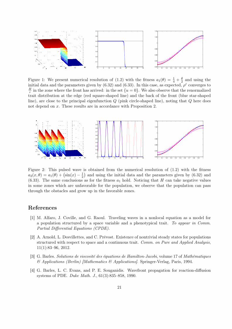
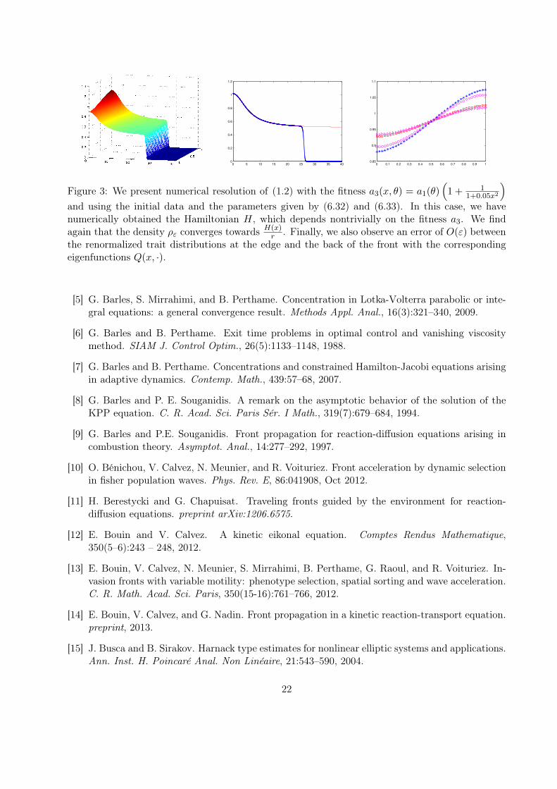
In Figure 2, we illustrate an example where H is periodic in x and it can take negative values.This corresponds to a case where the population faces some obstacles, i.e. zones where the conditionsare not favorable for the population to persist. However, according to the numerical illustrations,the population manages to pass through the obstacles and reach the favorable zones where it cangrow up again. Indeed, even if asymptotically as ε → 0 the density nε goes to 0 in these harshzones, in the ε–level, nε is positive but exponentially small. This small density can reach the betterzones and grow up. See Figures 1, 2 and 3 for detailed comments.

Acknowledgment

S. M. wishes to thank Gaël Raoul for early discussions and computations on this problem.

20

0 5 10 15 20 25 30 35 400

0.1

0.2

0.3

0.4

0.5

0.6

0.7

0 0.1 0.2 0.3 0.4 0.5 0.6 0.7 0.8 0.9 10.92

0.94

0.96

0.98

1

1.02

1.04

Figure 1: We present numerical resolution of (1.2) with the fitness a1(θ) = 14 + θ

2 and using theinitial data and the parameters given by (6.32) and (6.33). In this case, as expected, ρε converges toHr in the zone where the front has arrived: in the set {u = 0}. We also observe that the renormalizedtrait distribution at the edge (red square-shaped line) and the back of the front (blue star-shapedline), are close to the principal eigenfunction Q (pink circle-shaped line), noting that Q here doesnot depend on x. These results are in accordance with Proposition 2.

0 5 10 15 20 25 30 35 400

0.1

0.2

0.3

0.4

0.5

0.6

0.7

0.8

0.9

1

0 0.1 0.2 0.3 0.4 0.5 0.6 0.7 0.8 0.9 10.92

0.94

0.96

0.98

1

1.02

1.04

Figure 2: This pulsed wave is obtained from the numerical resolution of (1.2) with the fitnessa2(x, θ) = a1(θ) +

(sin(x)− 1

2

)and using the initial data and the parameters given by (6.32) and

(6.33). The same conclusions as for the fitness a1 hold. Noticing that H can take negative valuesin some zones which are unfavorable for the population, we observe that the population can passthrough the obstacles and grow up in the favorable zones.

References

[1] M. Alfaro, J. Coville, and G. Raoul. Traveling waves in a nonlocal equation as a model fora population structured by a space variable and a phenotypical trait. To appear in Comm.Partial Differential Equations (CPDE).

[2] A. Arnold, L. Desvillettes, and C. Prévost. Existence of nontrivial steady states for populationsstructured with respect to space and a continuous trait. Comm. on Pure and Applied Analysis,11(1):83–96, 2012.

[3] G. Barles. Solutions de viscosité des équations de Hamilton-Jacobi, volume 17 of Mathématiques& Applications (Berlin) [Mathematics & Applications]. Springer-Verlag, Paris, 1994.

[4] G. Barles, L. C. Evans, and P. E. Souganidis. Wavefront propagation for reaction-diffusionsystems of PDE. Duke Math. J., 61(3):835–858, 1990.

21

0 5 10 15 20 25 30 35 400

0.2

0.4

0.6

0.8

1

1.2

0 0.1 0.2 0.3 0.4 0.5 0.6 0.7 0.8 0.9 10.85

0.9

0.95

1

1.05

1.1

Figure 3: We present numerical resolution of (1.2) with the fitness a3(x, θ) = a1(θ)(

1 + 11+0.05x2

)and using the initial data and the parameters given by (6.32) and (6.33). In this case, we havenumerically obtained the Hamiltonian H, which depends nontrivially on the fitness a3. We findagain that the density ρε converges towards

H(x)r . Finally, we also observe an error of O(ε) between

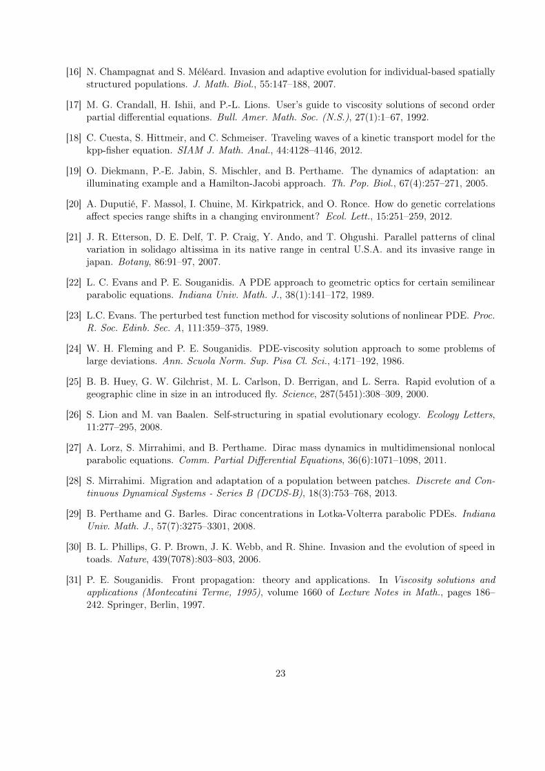
the renormalized trait distributions at the edge and the back of the front with the correspondingeigenfunctions Q(x, ·).

[5] G. Barles, S. Mirrahimi, and B. Perthame. Concentration in Lotka-Volterra parabolic or inte-gral equations: a general convergence result. Methods Appl. Anal., 16(3):321–340, 2009.

[6] G. Barles and B. Perthame. Exit time problems in optimal control and vanishing viscositymethod. SIAM J. Control Optim., 26(5):1133–1148, 1988.

[7] G. Barles and B. Perthame. Concentrations and constrained Hamilton-Jacobi equations arisingin adaptive dynamics. Contemp. Math., 439:57–68, 2007.

[8] G. Barles and P. E. Souganidis. A remark on the asymptotic behavior of the solution of theKPP equation. C. R. Acad. Sci. Paris Sér. I Math., 319(7):679–684, 1994.

[9] G. Barles and P.E. Souganidis. Front propagation for reaction-diffusion equations arising incombustion theory. Asymptot. Anal., 14:277–292, 1997.

[10] O. Bénichou, V. Calvez, N. Meunier, and R. Voituriez. Front acceleration by dynamic selectionin fisher population waves. Phys. Rev. E, 86:041908, Oct 2012.

[11] H. Berestycki and G. Chapuisat. Traveling fronts guided by the environment for reaction-diffusion equations. preprint arXiv:1206.6575.

[12] E. Bouin and V. Calvez. A kinetic eikonal equation. Comptes Rendus Mathematique,350(5–6):243 – 248, 2012.

[13] E. Bouin, V. Calvez, N. Meunier, S. Mirrahimi, B. Perthame, G. Raoul, and R. Voituriez. In-vasion fronts with variable motility: phenotype selection, spatial sorting and wave acceleration.C. R. Math. Acad. Sci. Paris, 350(15-16):761–766, 2012.

[14] E. Bouin, V. Calvez, and G. Nadin. Front propagation in a kinetic reaction-transport equation.preprint, 2013.

[15] J. Busca and B. Sirakov. Harnack type estimates for nonlinear elliptic systems and applications.Ann. Inst. H. Poincaré Anal. Non Linéaire, 21:543–590, 2004.

22

[16] N. Champagnat and S. Méléard. Invasion and adaptive evolution for individual-based spatiallystructured populations. J. Math. Biol., 55:147–188, 2007.

[17] M. G. Crandall, H. Ishii, and P.-L. Lions. User’s guide to viscosity solutions of second orderpartial differential equations. Bull. Amer. Math. Soc. (N.S.), 27(1):1–67, 1992.

[18] C. Cuesta, S. Hittmeir, and C. Schmeiser. Traveling waves of a kinetic transport model for thekpp-fisher equation. SIAM J. Math. Anal., 44:4128–4146, 2012.

[19] O. Diekmann, P.-E. Jabin, S. Mischler, and B. Perthame. The dynamics of adaptation: anilluminating example and a Hamilton-Jacobi approach. Th. Pop. Biol., 67(4):257–271, 2005.

[20] A. Duputié, F. Massol, I. Chuine, M. Kirkpatrick, and O. Ronce. How do genetic correlationsaffect species range shifts in a changing environment? Ecol. Lett., 15:251–259, 2012.

[21] J. R. Etterson, D. E. Delf, T. P. Craig, Y. Ando, and T. Ohgushi. Parallel patterns of clinalvariation in solidago altissima in its native range in central U.S.A. and its invasive range injapan. Botany, 86:91–97, 2007.

[22] L. C. Evans and P. E. Souganidis. A PDE approach to geometric optics for certain semilinearparabolic equations. Indiana Univ. Math. J., 38(1):141–172, 1989.

[23] L.C. Evans. The perturbed test function method for viscosity solutions of nonlinear PDE. Proc.R. Soc. Edinb. Sec. A, 111:359–375, 1989.

[24] W. H. Fleming and P. E. Souganidis. PDE-viscosity solution approach to some problems oflarge deviations. Ann. Scuola Norm. Sup. Pisa Cl. Sci., 4:171–192, 1986.

[25] B. B. Huey, G. W. Gilchrist, M. L. Carlson, D. Berrigan, and L. Serra. Rapid evolution of ageographic cline in size in an introduced fly. Science, 287(5451):308–309, 2000.

[26] S. Lion and M. van Baalen. Self-structuring in spatial evolutionary ecology. Ecology Letters,11:277–295, 2008.

[27] A. Lorz, S. Mirrahimi, and B. Perthame. Dirac mass dynamics in multidimensional nonlocalparabolic equations. Comm. Partial Differential Equations, 36(6):1071–1098, 2011.

[28] S. Mirrahimi. Migration and adaptation of a population between patches. Discrete and Con-tinuous Dynamical Systems - Series B (DCDS-B), 18(3):753–768, 2013.

[29] B. Perthame and G. Barles. Dirac concentrations in Lotka-Volterra parabolic PDEs. IndianaUniv. Math. J., 57(7):3275–3301, 2008.

[30] B. L. Phillips, G. P. Brown, J. K. Webb, and R. Shine. Invasion and the evolution of speed intoads. Nature, 439(7078):803–803, 2006.

[31] P. E. Souganidis. Front propagation: theory and applications. In Viscosity solutions andapplications (Montecatini Terme, 1995), volume 1660 of Lecture Notes in Math., pages 186–242. Springer, Berlin, 1997.

23