A 1.488 Approximation Algorithm for theUncapacitated Facility Location Problem

Shi Lia,1

aDepartment of Computer Science, Princeton University, Princeton, NJ, USA, 08540

Abstract

We present a 1.488-approximation algorithm for the metric uncapacitated

facility location (UFL) problem. Previously, the best algorithm was due to

Byrka (2007). Byrka proposed an algorithm parametrized by γ and used it

with γ ≈ 1.6774. By either running his algorithm or the algorithm proposed by

Jain, Mahdian and Saberi (STOC ’02), Byrka obtained an algorithm that gives

expected approximation ratio 1.5. We show that if γ is randomly selected, the

approximation ratio can be improved to 1.488. Our algorithm cuts the gap with

the 1.463 approximability lower bound by almost 1/3.

Keywords: Approximation, Facility Location Problem, Theory

1. Introduction

In this paper, we present an improved approximation algorithm for the (met-

ric) uncapacitated facility location (UFL) problem. In the UFL problem, we are

given a set of potential facility locations F , each i ∈ F with a facility cost fi, a

set of clients C and a metric d over F ∪ C. The goal is to find a subset F ′ ⊆ F

of locations to open facilities, to minimize the sum of the total facility cost and

the connection cost. The total facility cost is∑i∈F ′

fi, and the connection cost is∑j∈C

d(j, ij), where ij is the closest facility in F ′ to j.

1This research was supported by NSF awards MSPA-MCS 0528414, CCF 0832797, and AF0916218

Preprint submitted to Information and Computation September 8, 2011

The UFL problem is NP-hard and has received a lot of attention. In 1982,

Hochbaum [5] presented a greedy algorithm with O(log n)-approximation guar-

antee. Shmoys, Tardos and Aardal [12] used the filtering technique of Lin and

Vitter [10] to give a 3.16-approximation algorithm, which is the first constant

factor approximation. After that, a large number of constant factor approxi-

mation algorithms were proposed [4, 9, 3, 7, 8, 11]. The current best known

approximation ratio for the UFL problem is 1.50, given by Byrka [1].

On the negative side, Guha and Kuller [6] showed that there is no ρ-approximation

for the UFL problem if ρ < 1.463, unless NP ⊆ DTIME(nO(log logn)

). Later,

Sviridenko [13] strengthened the result by changing the condition to “unless

NP = P”. Jain et al. [8] generalized the result to show that no (γf , γc)-bifactor

approximation exists for γc < 1 + 2e−γf unless NP ⊆ DTIME(nO(log logn)

).

An algorithm is a (γf , γc)-approximation algorithm if the solution given by the

algorithm has expected total cost at most γfF∗ + γcC

∗, where F ∗ and C∗ are

the facility and the connection cost of an optimal solution for the linear pro-

gramming relaxation of the UFL problem described later, respectively.

Building on the work of Byrka [1], we give a 1.488-approximation algorithm

for the UFL problem. Byrka presented an algorithm A1(γ) which gives the opti-

mal bifactor approximation (γ, 1+2e−γ) for γ ≥ γ0 ≈ 1.6774. By either running

A1(γ0) or the (1.11, 1.78)-approximation algorithm A2 proposed by Jain, Mah-

dian and Saberi [8], Byrka was able to give a 1.5-approximation algorithm. We

show that the approximation ratio can be improved to 1.488 if γ is randomly

selected. To be more specific, we show

Theorem 1. There is a distribution over [1,∞) ∪ {⊥} such that the following

random algorithm for the UFL problem gives a solution whose expected cost is

at most 1.488 times the cost of the optimal solution : we randomly choose a

γ from the distribution; if γ =⊥, return the solution given by A2; otherwise,

return the solution given by A1(γ).

Due to the (γ, 1+2e−γ)-hardness result given by [8], there is a hard instance

for the algorithm A1(γ) for every γ. Roughly speaking, we show that a fixed

2

instance can not be hard for two different γ’s. Guided by this fact, we first give

a bifactor approximation ratio for A1(γ) that depends on the input instance and

then introduce a 0-sum game that characterizes the approximation ratio of our

algorithm. The game is between an algorithm designer and an adversary. The

algorithm designer plays either A1(γ) for some γ ≥ 1 or A2, while the adversary

plays an input instance for the UFL problem. By giving an explicit (mixed)

strategy for the algorithm designer, we show that the value of the game is at

most 1.488.

In Section 2, we review the algorithm A1(γ), and then give our improvement

in Section 3.

2. Review of the Algorithm A1(γ) in [1]

In this section, we review the (γ, 1+2e−γ)-bifactor approximation algorithm

A1(γ) for γ ≥ γ0 ≈ 1.67736 in [1].

In A1(γ) we first solve the following natural linear programming relaxation

for the UFL problem.

min∑

i∈F,j∈Cd(i, j)xi,j +

∑i∈F

fiyi s.t.

∑i∈F

xi,j = 1 ∀j ∈ C (1)

xi,j − yi ≤ 0 ∀i ∈ F ,j ∈ C (2)

xi,j , yi ≥ 0 ∀i ∈ F ,j ∈ C (3)

In the integer programming correspondent to the above LP relaxation, xi,j , yi ∈

{0, 1} for every i ∈ F and j ∈ C. yi indicates whether the facility i is open and

xi,j indicates whether the client j is connected to the facility i. Equation (1)

says that the client j must be connected to some facility and Inequality (2) says

that a client j can be connected to a facility i only if i is open.

If the y-variables are fixed, x-variables can be assigned greedily in the fol-

lowing way. Initially, xi,j = 0. For each client j ∈ C, run the following steps.

3

Sort facilities by their distances to j; then for each facility i in the order, assign

xij = yi if∑i′∈F xi′,j + yi ≤ 1 and xi,j = 1−

∑i′ xi′,j otherwise.

After obtaining a solution (x, y), we modify it by scaling the y-variables up

by a constant factor γ ≥ 1. Let y be the scaled vector of y-variables. We reassign

x-variables using the above greedy process to obtain a new solution (x, y).

Without loss of generality, we can assume that the following conditions hold

for every i ∈ C and j ∈ F :

1. xi,j ∈ {0, yi};

2. xi,j ∈ {0, yi};

3. yi ≤ 1.

Indeed, the above conditions can be guaranteed by splitting facilities. To

guarantee the first condition, we split i into 2 co-located facilities i′ and i′′ and

let xi′,j = yi′ = xi,j , yi′′ = yi − xi,j and xi′′,j = 0, if we find some facility i ∈ F

and client j ∈ C with 0 < xi,j < yi. The other x variables associated with i′ and

i′′ can be assigned naturally. We update x and y variables accordingly. Similarly,

we can guarantee the second condition. To guarantee the third condition, we can

split a facility i into 2 co-located facilities i′ and i′′ with yi′ = 1 and yi′′ = yi−1,

if we find some facility i ∈ F with yi > 1.

Definition 2 (volume). For some subset F ′ ⊆ F of facilities, define the vol-

ume of F ′, denoted by vol(F ′), to be the sum of yi over all facilities i ∈ F ′. i.e,

vol(F ′) =∑i∈F ′ yi.

Definition 3 (close and distant facilities). For a client j ∈ C, we say a

facility i is one of its close facilities if xi,j > 0. If xi,j = 0, but xi,j > 0, then

we say i is a distant facility of client j. Let FCj and FDj be the set of close and

distant facilities of j, respectively. Let Fj = FCj ∪ FDj .

Definition 4. For a client j ∈ C and a subset F ′ ⊆ F of facilities, define

d(j,F ′) to be the average distance of j to facilities in F ′, with respect to the

weights y. Recalling that y is a scaled vector of y, the average distances are also

4

with respect to the weights y. i.e,

d(j,F ′) =

∑i∈F ′ yid(j, i)∑

i∈F ′ yi=

∑i∈F ′ yid(j, i)∑

i∈F ′ yi.

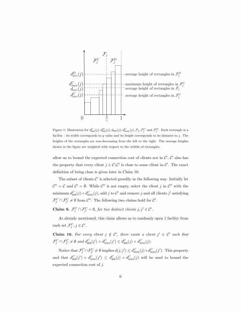
Definition 5 (dCave(j), dDave(j), dave(j) and dCmax(j)). For a client j ∈ C, define

dCave(j), dDave(j) and dave(j) to be the average distance from j to FCj ,FDj and Fj

respectively. i.e, dCave(j) = d(j,FCj ), dDave(j) = d(j,FDj ) and dave(j) = d(j,Fj).

Define dCmax(j) to be maximum distance from j to a facility in FCj .

By definition, dave(j) is the connection cost of j in the optimal fractional

solution. See Figure 1 for illustration of the above 3 definitions. The following

claims hold by the definitions of the corresponding quantities, and will be used

repeatedly later :

Claim 6. dCave(j) ≤ dCmax(j) ≤ dDave(j) and dCave(j) ≤ dave(j) ≤ dDave(j), for all

clients j ∈ C.

Claim 7. dave(j) =1

γdCave(j) +

γ − 1

γdDave(j), for all clients j ∈ C.

Claim 8. vol(FCj ) = 1, vol(FDj ) = γ − 1 and vol(Fj) = γ, for all clients j ∈ C.

Recall that yi indicates that whether the facility i is open. If we are aiming

at a (γ, γ)-bifactor approximation, we can open i with probability γyi = yi.

Then, the expected opening cost is exactly γ times that of the optimal fractional

solution. If by luck the sets FCj , j ∈ C are disjoint, the following simple algorithm

gives a (γ, 1)-bifactor approximation. Open exactly 1 facility in FCj , with yi

being the probability of opening i. (Recall that∑i∈FCj

yi = vol(FCj ) = 1.)

Connect each client j to its closest open facility. This is indeed a (γ, 1)-bifactor

approximation since the expected connection cost of j given by the algorithm

is dCave(j) ≤ dave(j).

In general, the sets FCj , j ∈ C may not be disjoint. In this case, we can not

randomly select 1 open facility from every FCj , since a facility i belonging to two

different FCj ’s would be open with probability more than yi. To overcome this

problem, we shall select a subset C′ ⊆ C of clients such that the sets FCj , j ∈ C′

are disjoint. We randomly open a facility in FCj only for facilities j ∈ C′. To

5

average height of rectangles in FCj

0

dCmax(j)

1

FCj FD

j

dave(j)

dDave(j)

dCave(j)

1γ

Fj

average height of rectangles in FDj

maximum height of rectangles in FCjaverage height of rectangles in Fj

Figure 1: Illustration for dCave(j), dDave(j), dave(j), d

Cmax(j),Fj ,FC

j and FDj . Each rectangle is a

facility : its width corresponds to y value and its height corresponds to its distance to j. The

heights of the rectangles are non-decreasing from the left to the right. The average heights

shown in the figure are weighted with respect to the widths of rectangles.

allow us to bound the expected connection cost of clients not in C′, C′ also has

the property that every client j ∈ C\C′ is close to some client in C′. The exact

definition of being close is given later in Claim 10.

The subset of clients C′ is selected greedily in the following way. Initially let

C′′ = C and C′ = ∅. While C′′ is not empty, select the client j in C′′ with the

minimum dCave(j)+dCmax(j), add j to C′ and remove j and all clients j′ satisfying

FCj ∩ FCj′ 6= ∅ from C′′. The following two claims hold for C′.

Claim 9. FCj ∩ FCj′ = ∅, for two distinct clients j, j′ ∈ C′.

As already mentioned, this claim allows us to randomly open 1 facility from

each set FCj , j ∈ C′.

Claim 10. For every client j /∈ C′, there exists a client j′ ∈ C′ such that

FCj ∩ FCj′ 6= ∅ and dCave(j′) + dCmax(j′) ≤ dCave(j) + dCmax(j).

Notice that FCj ∩FCj′ 6= ∅ implies d(j, j′) ≤ dCmax(j)+dCmax(j′). This property

and that dCave(j′) + dCmax(j′) ≤ dCave(j) + dCmax(j) will be used to bound the

expected connection cost of j.

6

Definition 11 (cluster center). For a client j /∈ C′, the client j′ ∈ C that

makes Claim 10 hold is called the cluster center of j.

We now randomly round the fractional solution (x, y). As we already men-

tioned, for each j ∈ C′, we open exactly one of its close facilities randomly with

probabilities yi. For each facility i that is not a close facility of any client in

C′, we open it independently with probability yi. Connect each client j to its

closest open facility and let Cj be its connection cost.

Since i is open with probability exactly yi for every facility i ∈ F , the

expected opening cost of the solution given by the above algorithm is exactly γ

times that of the optimal fractional solution. If j ∈ C′ then E[Cj ] = dCave(j) ≤

dave(j).

Byrka in [1] showed that for every client j /∈ C′,

1. The probability that some facility in FCj (resp., FDj ) is open is at least

1 − e−vol(FCj ) = 1 − e−1(resp., 1 − e−vol(F

Dj ) = 1 − e−(γ−1)), and under

the condition that the event happens, the expected distance between j

and the closest open facility in FCj (resp., FDj ) is at most dCave(j) (resp.,

dDave(j));

2. d(j,FCj′ \Fj) ≤ dDave(j) + dCmax(j) + dCave(j)(recall that d(j,FCj′ \Fj) is the

weighted average distance from j to facilities in FCj′ \Fj), where j′ is the

cluster center of j; or equivalently, under the condition that there is no

open facility in Fj , the expected distance between j and the unique open

facility in FCj′ is at most dDave(j) + dCmax(j) + dCave(j).

Since dCave(j) ≤ dDave(j) ≤ dDave(j) + dCmax(j) + dCave(j), we have

E[Cj ] ≤ (1− e−1)dCave(j) + e−1(1− e−(γ−1))dDave(j)

+ e−1e−(γ−1)(dDave(j) + dCmax(j) + dCave(j))

= (1− e−1 + e−γ)dCave(j) + e−1dDave(j) + e−γdCmax(j)

≤ (1− e−1 + e−γ)dCave(j) + (e−1 + e−γ)dDave(j). (4)

Notice that the connection cost of j in the optimal fractional solution is dave(j) =1

γdCave(j) +

γ − 1

γdDave(j). We compute the maximum ratio between (1 − e−1 +

7

e−γ)dCave(j) + (e−1 + e−γ)dDave(j) and1

γdCave(j) +

γ − 1

γdDave(j). Since dCave(j) ≤

dDave(j), the ratio is maximized when dCave(j) = dDave(j) > 0 or dDave(j) > dCave(j) =

0. For γ ≥ γ0, the maximum ratio is achieved when dCave(j) = dDave(j) > 0,

in which case the maximum is 1 + 2e−γ . Thus, the algorithm A1(γ0) gives a

(γ0 ≈ 1.67736, 1 + 2e−γ0 ≈ 1.37374)-bifactor approximation.2

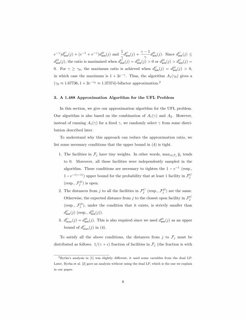
3. A 1.488 Approximation Algorithm for the UFL Problem

In this section, we give our approximation algorithm for the UFL problem.

Our algorithm is also based on the combination of A1(γ) and A2. However,

instead of running A1(γ) for a fixed γ, we randomly select γ from some distri-

bution described later.

To understand why this approach can reduce the approximation ratio, we

list some necessary conditions that the upper bound in (4) is tight.

1. The facilities in Fj have tiny weights. In other words, maxi∈Fj yi tends

to 0. Moreover, all these facilities were independently sampled in the

algorithm. These conditions are necessary to tighten the 1 − e−1 (resp.,

1− e−(γ−1)) upper bound for the probability that at least 1 facility in FCj(resp., FDj ) is open.

2. The distances from j to all the facilities in FCj (resp., FDj ) are the same.

Otherwise, the expected distance from j to the closest open facility in FCj(resp., FDj ), under the condition that it exists, is strictly smaller than

dCave(j) (resp., dDave(j)).

3. dCmax(j) = dDave(j). This is also required since we used dDave(j) as an upper

bound of dCmax(j) in (4).

To satisfy all the above conditions, the distances from j to Fj must be

distributed as follows. 1/(γ + ε) fraction of facilities in Fj (the fraction is with

2Byrka’s analysis in [1] was slightly different; it used some variables from the dual LP.

Later, Byrka et al. [2] gave an analysis without using the dual LP, which is the one we explain

in our paper.

8

respect to the weights yi.) have distances a to j, and the other 1 − 1/(γ + ε)

fraction have distances b ≥ a to j. For ε tending to 0, dCave(j) = a and dCmax(j) =

dDave(j) = b.

As discussed earlier, if a = b, then E[Cj ]/dave(j) ≤ 1 + 2e−γ . Intuitively, the

bad cases should have a � b. However, if we replace γ with γ + 1.01ε (say),

then dCmax(j) will equal dCave(j) = a, instead of dDave(j) = b. Thus, we can greatly

reduce the approximation ratio if the distributions for all j’s are of the above

form.

Hence, using only two different γ’s, we are already able to make an improve-

ment. To give a better analysis, we first give in Section 3.1 an upper bound on

E[Cj ], in terms of the distribution of distances from j to Fj , not just dCave(j) and

dDave(j) and then give in Section 3.2 an explicit distribution for γ by introducing

a 0-sum game.

3.1. Upper-Bounding the Expected Connection Cost of a Client

We bound E[Cj ] in this subsection. It suffices to assume j /∈ C′, since

we can think of a client j ∈ C′ as a client j /∈ C′ which has a co-located client

j′ ∈ C′. Similar to [1], we first give an upper bound on d(j,FCj′ \Fj) in Lemma 12.

The bound and the proof are the same as the counterparts in [1], except that

we made a slight improvement. The improvement is not essential to the final

approximation ratio; however, it will simplify the analytical proof in Section 3.2.

Lemma 12. For some client j /∈ C′, let j′ be the cluster center of j. So

j′ ∈ C′,FCj ∩ FCj′ 6= ∅ and dCave(j′) + dCmax(j′) ≤ dCave(j) + dCmax(j). We have,

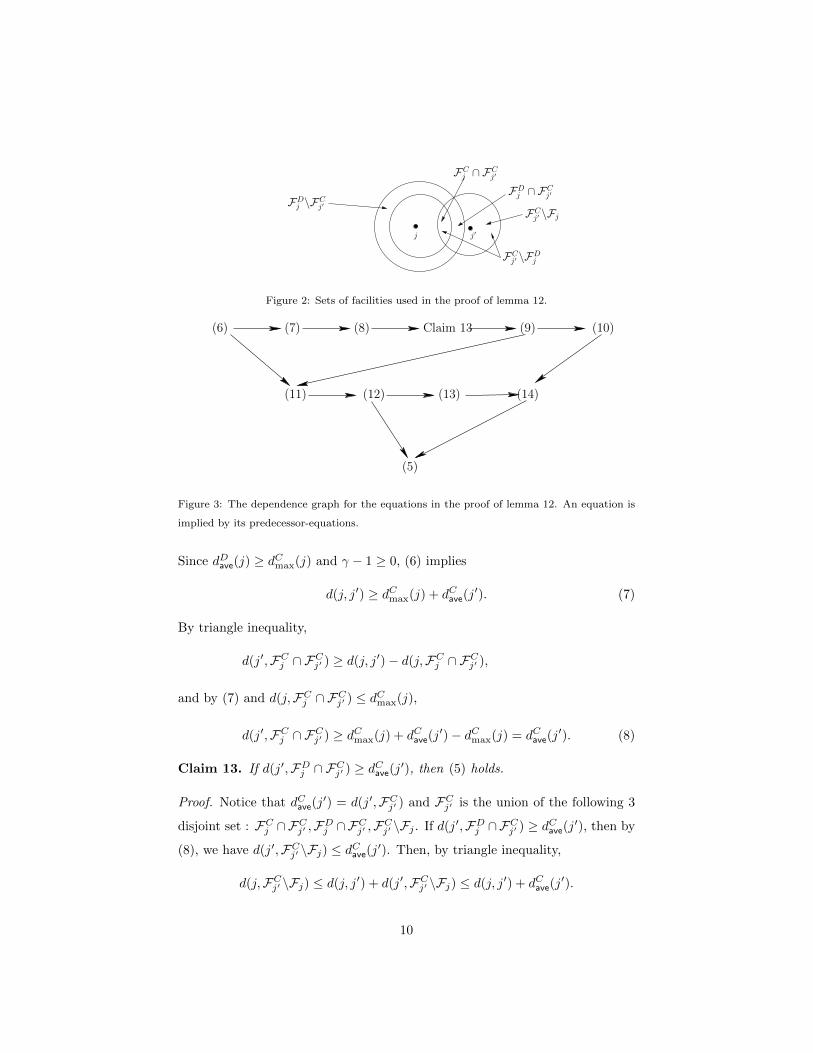
d(j,FCj′ \Fj) ≤ (2− γ)dCmax(j) + (γ − 1)dDave(j) + dCmax(j′) + dCave(j′). (5)

Proof. Figure 2 illustrates the sets of facilities we are going to use. Figure 3

shows the dependence of equations we shall prove and can be viewed as the

outline of the proof.

If d(j, j′) ≤ (2−γ)dCmax(j) + (γ− 1)dDave(j) +dCave(j′), the remaining dCmax(j′)

is enough for the distance between j′ and any facility in FCj′ . So, we will assume

d(j, j′) ≥ (2− γ)dCmax(j) + (γ − 1)dDave(j) + dCave(j′). (6)

9

FDj \FC

j′

FCj ∩ FC

j′

FDj ∩ FC

j′

j j′

FCj′ \Fj

FCj′ \FD

j

Figure 2: Sets of facilities used in the proof of lemma 12.

Claim 13(6) (9) (10)

(11) (12) (13) (14)

(5)

(7) (8)

Figure 3: The dependence graph for the equations in the proof of lemma 12. An equation is

implied by its predecessor-equations.

Since dDave(j) ≥ dCmax(j) and γ − 1 ≥ 0, (6) implies

d(j, j′) ≥ dCmax(j) + dCave(j′). (7)

By triangle inequality,

d(j′,FCj ∩ FCj′ ) ≥ d(j, j′)− d(j,FCj ∩ FCj′ ),

and by (7) and d(j,FCj ∩ FCj′ ) ≤ dCmax(j),

d(j′,FCj ∩ FCj′ ) ≥ dCmax(j) + dCave(j′)− dCmax(j) = dCave(j

′). (8)

Claim 13. If d(j′,FDj ∩ FCj′ ) ≥ dCave(j′), then (5) holds.

Proof. Notice that dCave(j′) = d(j′,FCj′ ) and FCj′ is the union of the following 3

disjoint set : FCj ∩FCj′ ,FDj ∩FCj′ ,FCj′ \Fj . If d(j′,FDj ∩FCj′ ) ≥ dCave(j′), then by

(8), we have d(j′,FCj′ \Fj) ≤ dCave(j′). Then, by triangle inequality,

d(j,FCj′ \Fj) ≤ d(j, j′) + d(j′,FCj′ \Fj) ≤ d(j, j′) + dCave(j′).

10

Since FCj ∩ FCj′ 6= ∅,

d(j,FCj′ \Fj) ≤ dCmax(j) + dCmax(j′) + dCave(j′)

≤ (2− γ)dCmax(j) + (γ − 1)dDave(j) + dCmax(j′) + dCave(j′).

This proves the claim.

So, we can also assume

d(j′,FDj ∩ FCj′ ) = dCave(j′)− z (9)

for some positive z. Let y = vol(FDj ∩ FCj′ ). Notice that y ≤ max {γ − 1, 1}.

Since dCave(j′) = yd(j′,FDj ∩ FCj′ ) + (1− y)d(j′,FCj′ \FDj ), we have

d(j′,FCj′ \FDj ) = dCave(j′) +

y

1− yz. (10)

By (6), (9) and triangle inequality, we have

d(j,FDj ∩ FCj′ ) ≥ d(j, j′)− d(j′,FCj′ ∩ FDj )

≥ (2− γ)dCmax(j) + (γ − 1)dDave(j) + dCave(j′)− (dCave(j

′)− z)

= dDave(j)− (2− γ)(dDave(j)− dCmax(j)) + z. (11)

Noticing that dDave(j) =y

γ − 1d(j,FDj ∩ FCj′ ) +

γ − 1− yγ − 1

d(j,FDj \FCj′ ), we

have

− y

γ − 1

(d(j,FDj ∩ FCj′ )− dDave(j)

)=γ − 1− yγ − 1

(d(j,FDj \FCj′ )− dDave(j)

).

Thus,

d(j,FDj \FCj′ ) = dDave(j)−y

γ − 1− y(d(j,FDj ∩ FCj′ )− dDave(j)

).

Then, by dCmax(j) ≤ d(j,FDj \FCj′ ) and (11),

dCmax(j) ≤ d(j,FDj \FCj′ ) ≤ dDave(j)−y

γ − 1− y(z − (2− γ)(dDave(j)− dCmax(j))

).

So,

dDave(j)− dCmax(j) ≥ y

γ − 1− y(z − (2− γ)(dDave(j)− dCmax(j))

),

11

and since 1 +(2− γ)y

γ − 1− y=

(γ − 1)(1− y)

γ − 1− y≥ 0,

dDave(j)− dCmax(j) ≥ y

γ − 1− yz/(

1 +(2− γ)y

γ − 1− y

)=

yz

(γ − 1)(1− y). (12)

By triangle inequality,

d(j′,FCj ∩ FCj′ ) ≥ d(j, j′)− d(j,FCj ∩ FCj′ ),

and by (6) and d(j,FCj ∩ FCj′ ) ≤ dCmax(j),

d(j′,FCj ∩ FCj′ ) ≥ (2− γ)dCmax(j) + (γ − 1)dDave(j) + dCave(j′)− dCmax(j)

= (γ − 1)(dDave(j)− dCmax(j)) + dCave(j′).

Then by (12), we have

d(j′,FCj ∩ FCj′ ) ≥y

1− yz + dCave(j

′). (13)

Notice that FCj′ \FDj is the union of the following two sets : FCj ∩FCj′ and FCj′ \Fj .

Combining (10) and (13), we have

d(j′,FCj′ \Fj) ≤ dCave(j′) +y

1− yz. (14)

So,

d(j,FCj′ \Fj) ≤ dCmax(j) + dCmax(j′) + d(j′,FCj′ \Fj)

= (2− γ)dCmax(j) + (γ − 1)dCmax(j) + dCmax(j′) + d(j′,FCj′ \Fj)

by (12) and (14),

≤ (2− γ)dCmax(j) + (γ − 1)

(dDave(j)−

yz

(γ − 1)(1− y)

)+ dCmax(j′) + dCave(j

′) +yz

1− y

= (2− γ)dCmax(j) + (γ − 1)dDave(j) + dCmax(j′) + dCave(j′).

12

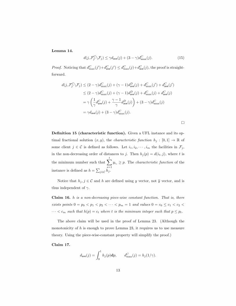
Lemma 14.

d(j,FCj′ \Fj) ≤ γdave(j) + (3− γ)dCmax(j). (15)

Proof. Noticing that dCmax(j′)+dCave(j′) ≤ dCmax(j)+dCave(j), the proof is straight-

forward.

d(j,FCj′ \Fj) ≤ (2− γ)dCmax(j) + (γ − 1)dDave(j) + dCmax(j′) + dCave(j′)

≤ (2− γ)dCmax(j) + (γ − 1)dDave(j) + dCmax(j) + dCave(j)

= γ

(1

γdCave(j) +

γ − 1

γdDave(j)

)+ (3− γ)dCmax(j)

= γdave(j) + (3− γ)dCmax(j).

Definition 15 (characteristic function). Given a UFL instance and its op-

timal fractional solution (x, y), the characteristic function hj : [0, 1] → R of

some client j ∈ C is defined as follows. Let i1, i2, · · · , im the facilities in Fj ,

in the non-decreasing order of distances to j. Then hj(p) = d(it, j), where t is

the minimum number such that

t∑s=1

yis ≥ p. The characteristic function of the

instance is defined as h =∑j∈C hj .

Notice that hj , j ∈ C and h are defined using y vector, not y vector, and is

thus independent of γ.

Claim 16. h is a non-decreasing piece-wise constant function. That is, there

exists points 0 = p0 < p1 < p2 < · · · < pm = 1 and values 0 = c0 ≤ c1 < c2 <

· · · < cm such that h(p) = ct where t is the minimum integer such that p ≤ pt.

The above claim will be used in the proof of Lemma 23. (Although the

monotonicity of h is enough to prove Lemma 23, it requires us to use measure

theory. Using the piece-wise-constant property will simplify the proof.)

Claim 17.

dave(j) =

∫ 1

0

hj(p)dp, dCmax(j) = hj(1/γ).

13

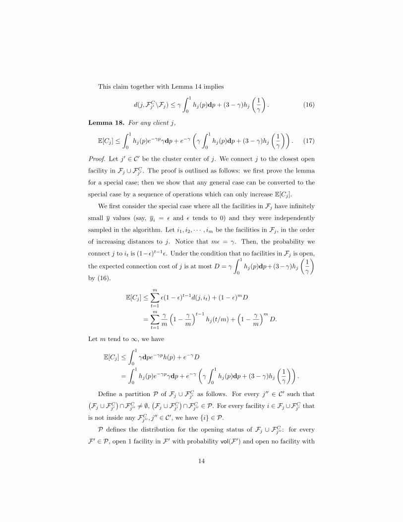
This claim together with Lemma 14 implies

d(j,FCj′ \Fj) ≤ γ∫ 1

0

hj(p)dp+ (3− γ)hj

(1

γ

). (16)

Lemma 18. For any client j,

E[Cj ] ≤∫ 1

0

hj(p)e−γpγdp+ e−γ

(γ

∫ 1

0

hj(p)dp+ (3− γ)hj

(1

γ

)). (17)

Proof. Let j′ ∈ C′ be the cluster center of j. We connect j to the closest open

facility in Fj ∪ FCj′ . The proof is outlined as follows: we first prove the lemma

for a special case; then we show that any general case can be converted to the

special case by a sequence of operations which can only increase E[Cj ].

We first consider the special case where all the facilities in Fj have infinitely

small y values (say, yi = ε and ε tends to 0) and they were independently

sampled in the algorithm. Let i1, i2, · · · , im be the facilities in Fj , in the order

of increasing distances to j. Notice that mε = γ. Then, the probability we

connect j to it is (1−ε)t−1ε. Under the condition that no facilities in Fj is open,

the expected connection cost of j is at most D = γ

∫ 1

0

hj(p)dp+(3−γ)hj

(1

γ

)by (16).

E[Cj ] ≤m∑t=1

ε(1− ε)t−1d(j, it) + (1− ε)mD

=

m∑t=1

γ

m

(1− γ

m

)t−1hj(t/m) +

(1− γ

m

)mD.

Let m tend to ∞, we have

E[Cj ] ≤∫ 1

0

γdpe−γph(p) + e−γD

=

∫ 1

0

hj(p)e−γpγdp+ e−γ

(γ

∫ 1

0

hj(p)dp+ (3− γ)hj

(1

γ

)).

Define a partition P of Fj ∪ FCj′ as follows. For every j′′ ∈ C′ such that(Fj ∪ FCj′

)∩FCj′′ 6= ∅,

(Fj ∪ FCj′

)∩FCj′′ ∈ P. For every facility i ∈ Fj ∪FCj′ that

is not inside any FCj′′ , j′′ ∈ C′, we have {i} ∈ P.

P defines the distribution for the opening status of Fj ∪ FCj′′ : for every

F ′ ∈ P, open 1 facility in F ′ with probability vol(F ′) and open no facility with

14

probability 1− vol(F ′); the probability of opening i ∈ F ′ is yi; the sets in P are

handled independently.

Claim 19. If some subset F ′ ⊆ Fj\FCj′ ,F ′ ∈ P has |F ′| ≥ 2, removing F ′

from P and add |F ′| singular sets, each containing one facility in mF ′, to P

can only make E[Cj ] smaller.

Proof. For the sake of description, we only consider the case when |F ′| = 2.

The proof can be easily extended to the case where |F ′| ≥ 3.

Assume F ′ = {i, i′}, where i and i′ are two distinct facilities in Fj\FCj′ and

d(j, i) ≤ d(j, i′). Focus on the distribution for the distance D between j and

its closest open facility in {i, i′} (D = ∞ if it does not exist) before and after

splitting the set {i, i′}.

Before the splitting operation, the distribution is : with probability yi, D =

d(j, i), with probability yi′ , D = d(j, i′), and with probability 1 − yi − yi′ ,

D = ∞. After splitting, the distribution is: with probability yi, D = d(j, i),

with probability (1−yi)yi′ , D = d(j, i′) and with the probability (1−yi)(1−yi′),

D =∞. So, the distribution before splitting strictly dominates the distribution

after splitting. Thus, splitting {i, i′} can only increase E[Cj ].

Thus, we can assume P ={FCj′}⋃{

{i} : i ∈ Fj\FCj′}

. That is, facilities in

Fj\FCj′ are independently sampled. Then, we show that the following sequence

of operations can only increase E[Cj ].

1. Split the set FCj′ ∈ P into two subsets: FCj′ ∩ Fj , and FCj′ \Fj ;

2. Scale up y values in FCj′ \Fj so that the volume of FCj′ \Fj becomes 1.

Indeed, consider distribution for the distance between j and the closest open

facility in FCj′ . The distribution does not change after we performed the opera-

tions, since dmax(j,FCj′ ∩ Fj) ≤ dmin(j,FCj′ \Fj), where dmax and dmin denotes

the maximum and the minimum distance from a client to a set of facilities,

respectively.

Again, by Claim 19, we can split FCj′ ∩ Fj into singular sets. By the same

argument, splitting a facility i ∈ Fj into 2 facilities i′ and i′′ with yi = yi′ + yi′′

15

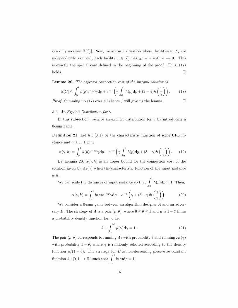
can only increase E[Cj ]. Now, we are in a situation where, facilities in Fj are

independently sampled, each facility i ∈ Fj has yi = ε with ε → 0. This

is exactly the special case defined in the beginning of the proof. Thus, (17)

holds.

Lemma 20. The expected connection cost of the integral solution is

E[C] ≤∫ 1

0

h(p)e−γpγdp+ e−γ(γ

∫ 1

0

h(p)dp+ (3− γ)h

(1

γ

)). (18)

Proof. Summing up (17) over all clients j will give us the lemma.

3.2. An Explicit Distribution for γ

In this subsection, we give an explicit distribution for γ by introducing a

0-sum game.

Definition 21. Let h : [0, 1) be the characteristic function of some UFL in-

stance and γ ≥ 1. Define

α(γ, h) =

∫ 1

0

h(p)e−γpγdp+ e−γ(γ

∫ 1

0

h(p)dp+ (3− γ)h

(1

γ

)). (19)

By Lemma 20, α(γ, h) is an upper bound for the connection cost of the

solution given by A1(γ) when the characteristic function of the input instance

is h.

We can scale the distances of input instance so that

∫ 1

0

h(p)dp = 1. Then,

α(γ, h) =

∫ 1

0

h(p)e−γpγdp+ e−γ(γ + (3− γ)h

(1

γ

)). (20)

We consider a 0-sum game between an algorithm designer A and an adver-

sary B. The strategy of A is a pair (µ, θ), where 0 ≤ θ ≤ 1 and µ is 1− θ times

a probability density function for γ. i.e,

θ +

∫ ∞1

µ(γ)dγ = 1. (21)

The pair (µ, θ) corresponds to running A2 with probability θ and running A1(γ)

with probability 1 − θ, where γ is randomly selected according to the density

function µ/(1 − θ). The strategy for B is non-decreasing piece-wise constant

function h : [0, 1]→ R∗ such that

∫ 1

0

h(p)dp = 1.

16

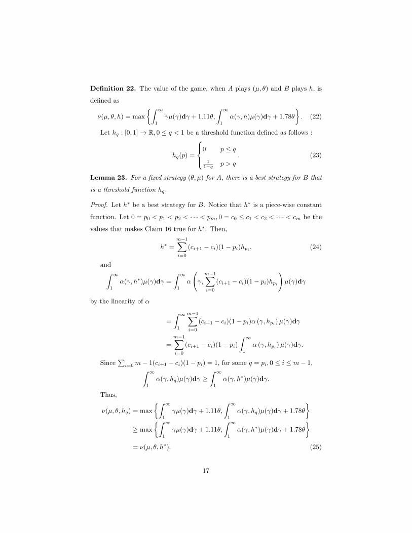
Definition 22. The value of the game, when A plays (µ, θ) and B plays h, is

defined as

ν(µ, θ, h) = max

{∫ ∞1

γµ(γ)dγ + 1.11θ,

∫ ∞1

α(γ, h)µ(γ)dγ + 1.78θ

}. (22)

Let hq : [0, 1]→ R, 0 ≤ q < 1 be a threshold function defined as follows :

hq(p) =

0 p ≤ q

11−q p > q

. (23)

Lemma 23. For a fixed strategy (θ, µ) for A, there is a best strategy for B that

is a threshold function hq.

Proof. Let h∗ be a best strategy for B. Notice that h∗ is a piece-wise constant

function. Let 0 = p0 < p1 < p2 < · · · < pm, 0 = c0 ≤ c1 < c2 < · · · < cm be the

values that makes Claim 16 true for h∗. Then,

h∗ =

m−1∑i=0

(ci+1 − ci)(1− pi)hpi , (24)

and∫ ∞1

α(γ, h∗)µ(γ)dγ =

∫ ∞1

α

(γ,

m−1∑i=0

(ci+1 − ci)(1− pi)hpi

)µ(γ)dγ

by the linearity of α

=

∫ ∞1

m−1∑i=0

(ci+1 − ci)(1− pi)α (γ, hpi)µ(γ)dγ

=

m−1∑i=0

(ci+1 − ci)(1− pi)∫ ∞1

α (γ, hpi)µ(γ)dγ.

Since∑i=0m− 1(ci+1 − ci)(1− pi) = 1, for some q = pi, 0 ≤ i ≤ m− 1,∫ ∞

1

α(γ, hq)µ(γ)dγ ≥∫ ∞1

α(γ, h∗)µ(γ)dγ.

Thus,

ν(µ, θ, hq) = max

{∫ ∞1

γµ(γ)dγ + 1.11θ,

∫ ∞1

α(γ, hq)µ(γ)dγ + 1.78θ

}≥ max

{∫ ∞1

γµ(γ)dγ + 1.11θ,

∫ ∞1

α(γ, h∗)µ(γ)dγ + 1.78θ

}= ν(µ, θ, h∗). (25)

17

This finishes the proof.

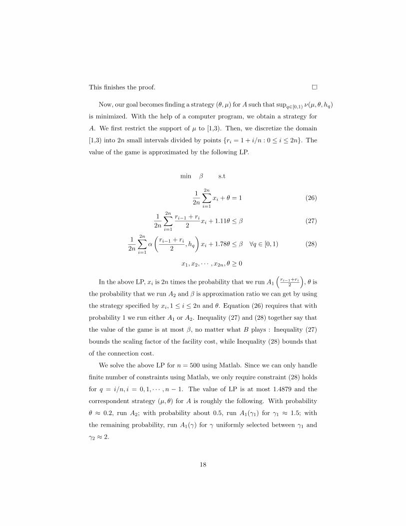
Now, our goal becomes finding a strategy (θ, µ) forA such that supq∈[0,1) ν(µ, θ, hq)

is minimized. With the help of a computer program, we obtain a strategy for

A. We first restrict the support of µ to [1,3). Then, we discretize the domain

[1,3) into 2n small intervals divided by points {ri = 1 + i/n : 0 ≤ i ≤ 2n}. The

value of the game is approximated by the following LP.

min β s.t

1

2n

2n∑i=1

xi + θ = 1 (26)

1

2n

2n∑i=1

ri−1 + ri2

xi + 1.11θ ≤ β (27)

1

2n

2n∑i=1

α

(ri−1 + ri

2, hq

)xi + 1.78θ ≤ β ∀q ∈ [0, 1) (28)

x1, x2, · · · , x2n, θ ≥ 0

In the above LP, xi is 2n times the probability that we run A1

(ri−1+ri

2

), θ is

the probability that we run A2 and β is approximation ratio we can get by using

the strategy specified by xi, 1 ≤ i ≤ 2n and θ. Equation (26) requires that with

probability 1 we run either A1 or A2. Inequality (27) and (28) together say that

the value of the game is at most β, no matter what B plays : Inequality (27)

bounds the scaling factor of the facility cost, while Inequality (28) bounds that

of the connection cost.

We solve the above LP for n = 500 using Matlab. Since we can only handle

finite number of constraints using Matlab, we only require constraint (28) holds

for q = i/n, i = 0, 1, · · · , n − 1. The value of LP is at most 1.4879 and the

correspondent strategy (µ, θ) for A is roughly the following. With probability

θ ≈ 0.2, run A2; with probability about 0.5, run A1(γ1) for γ1 ≈ 1.5; with

the remaining probability, run A1(γ) for γ uniformly selected between γ1 and

γ2 ≈ 2.

18

µ(γ)

γ1 γ2

a

γ

accumulated probability θ1

Figure 4: The distribution of γ. With probability θ1, we run A1(γ1); with probability a(γ2 −

γ1), we run A1(γ) with γ randomly selected from [γ1, γ2]; with probability θ2 = 1 − θ1 −

a(γ2 − γ1), we run A2.

In light of the program generated solution, we give a pure analytical strategy

for A and show that the value of the game is at most 1.488. The strategy (µ, θ)

is defined as follows. With probability θ = θ2, we run A2; with probability θ1,

we run A1(γ) with γ = γ1; with probability 1 − θ2 − θ1, we run A1(γ) with γ

randomly chosen between γ1 and γ2. Thus, the function µ is

µ(γ) = aIγ1,γ2(γ) + θ1δ(γ − γ1), (29)

where δ is the Dirac-Delta function, a =1− θ1 − θ2γ2 − γ1

, and Iγ1,γ2(γ) is 1 if γ1 <

γ < γ2 and 0 otherwise(See Figure 4). The values of θ1, θ2, γ1, γ2, a are given

later.

The remaining part of the paper is devoted to prove the following lemma.

Lemma 24. There exists some θ1 ≥ 0, θ2 ≥ 0, 1 ≤ γ1 < γ2 and a ≥ 0 such that

θ1 + θ2 + a(γ2 − γ1) = 1 and supq∈[0,1) ν(µ, θ, hq) ≤ 1.488.

Proof. The scaling factor for the facility cost is

γf = θ1γ1 + a(γ2 − γ1)γ1 + γ2

2+ 1.11θ2. (30)

Now, we consider the scaling factor γc when h = hq. By Lemma 20,

γc(q) ≤∫ ∞1

(∫ 1

0

e−γpγhq(p)dp+ e−γ(γ + (3− γ)hq(1/γ))

)µ(γ)dγ + 1.78θ2

19

replacing µ with aIγ1,γ2(γ)+θ1δ(γ−γ1) and hq(p) with 0 or 1/(1−q) depending

on whether p ≤ q,

=

∫ γ2

γ1

(∫ 1

q

e−γpγ1

1− qdp+ e−γγ + (3− γ)hq(1/γ)

)adγ

+ θ1

(∫ 1

q

e−γ1pγ11

1− qdp+ e−γ1(γ1 + (3− γ1)hq(1/γ1))

)+ 1.78θ2

= B1(q) +B2(q) +B3(q) + 1.78θ2, (31)

where

B1(q) =

∫ γ2

γ1

∫ 1

q

e−γpγ1

1− qdpadγ +

∫ γ2

γ1

e−γγadγ,

B2(q) =

∫ γ2

γ1

(3− γ)hq(1/γ)adγ,

and

B3(q) = θ1

∫ 1

q

e−γ1pγ11

1− qdp+ θ1e

−γ1(γ1 + (3− γ1)hq(1/γ1)).

Then, we calculate B1(q), B2(q) and B3(q) separately.

B1(q) =

∫ γ2

γ1

∫ 1

q

e−γpγ1

1− qdpadγ +

∫ γ2

γ1

e−γγadγ

=a

1− q

∫ γ2

γ1

(e−γq − e−γ)dγ − a(γ + 1)e−γ∣∣γ2γ1

=a

(1− q)q(e−γ1q − e−γ2q)− a

1− q(e−γ1 − e−γ2)

+ a((γ1 + 1)e−γ1 − (γ2 + 1)e−γ2).

(32)

B2(q) =

∫ γ2

γ1

(3− γ)hq(1/γ)adγ

=

a

1−q ((2− γ1)e−γ1 − (2− γ2)e−γ2) 0 ≤ q < 1/γ2

a1−q

((2− γ1)e−γ1 − (2− 1/q)e−1/q

)1/γ2 ≤ q ≤ 1/γ1

0 1/γ1 < q < 1

. (33)

20

B3(q) = θ1

∫ 1

q

e−γ1pγ11

1− qdp+ θ1e

−γ1(γ1 + (3− γ1)hq(1/γ1))

= θ1

(1

1− q(e−γ1q − e−γ1) + e−γ1γ1 + e−γ1(3− γ1)hq(1/γ1)

)

=

θ1(

11−q (e−γ1q − e−γ1) + e−γ1γ1 + e−γ1 (3−γ1)

1−q

)0 ≤ q ≤ 1/γ1

θ1

(1

1−q (e−γ1q − e−γ1) + e−γ1γ1

)1/γ1 < q < 1

.

(34)

So, we have 3 cases :

1. 0 ≤ q < 1/γ2.

γc(q) ≤ B1(q) +B2(q) +B3(q)

=a

(1− q)q(e−γ1q − e−γ2q)− a

1− q(e−γ1 − e−γ2)

+ a((γ1 + 1)e−γ1 − (γ2 + 1)e−γ2) +a

1− q((2− γ1)e−γ1 − (2− γ2)e−γ2

)+ θ1(

1

1− q(e−γ1q − e−γ1) + e−γ1γ1 +

1

1− qe−γ1(3− γ1)) + 1.78θ2

=a

(1− q)q(e−γ1q − e−γ2q) +

A1

1− q+ θ1

e−γ1q

1− q+A2,

where A1 = a(e−γ1 − γ1e−γ1 − e−γ2 + γ2e−γ2) + 2θ1e

−γ1 − θ1e−γ1γ1

and A2 = a((γ1 + 1)e−γ1 − (γ2 + 1)e−γ2) + θ1e−γ1γ1 + 1.78θ2.

2. 1/γ2 ≤ q ≤ 1/γ1.

The only difference between this case and the first case is the definition of

B2(q). Comparing the definition of B2(q) for the case 0 ≤ q < 1/γ2 and

the case 1/γ2 ≤ q ≤ 1/γ1, we can get

γc(q) =a

(1− q)q(e−γ1q − e−γ2q) +

A1

1− q+ θ1

e−γ1q

1− q+A2

+a

1− q

((2− γ2)e−γ2 − (2− 1/q)e−1/q

). (35)

21

0 0.5 10.8

0.9

1

1.1

1.2

1.3

1.4

1.5

0.5 0.55 0.6 0.651.4865

1.487

1.4875

1.488

Figure 5: The function γc(q). The curve on the right-hand side is the function restricted to

the interval (1/γ2, 1/γ1).

3. 1/γ1 < q < 1

γc(q) ≤a

(1− q)q(e−γ1q − e−γ2q)− a

1− q(e−γ1 − e−γ2)

+ a((γ1 + 1)e−γ1 − (γ2 + 1)e−γ2)

+ θ1

(1

1− q(e−γ1q − e−γ1) + e−γ1γ1

)+ 1.78θ2

=a

(1− q)q(e−γ1q − e−γ2q) +

A3

1− q+ θ1

e−γ1q

1− q+A2, (36)

where A3 = a(−e−γ1 + e−γ2)− θ1e−γ1 .

We set γ1 = 1.479311, γ2 = 2.016569, θ1 = 0.503357, a = 0.560365 and

θ2 = 1− θ1 − a(γ2 − γ1) ≈ 0.195583. Then,

γf = θ1γ1 + a(γ2 − γ1)γ1 + γ2

2+ 1.11θ2 ≈ 1.487954. (37)

A1 ≈ 0.074347, A2 ≈ 0.609228 and A3 ≈ −0.167720. γc(q) has the maximum

value about 1.487989, achieved at q = 0(see Figure 5). This finishes the proof

of Lemma 24.

Thus, Theorem 1 follows immediately from lemma Lemma 23 and Lemma 24.

Acknowledgements.

I thank Moses Charikar, my advisor, for helpful discussions.

22

[1] Jaroslaw Byrka. An optimal bifactor approximation algorithm for the met-

ric uncapacitated facility location problem. In APPROX ’07/RANDOM

’07: Proceedings of the 10th International Workshop on Approximation

and the 11th International Workshop on Randomization, and Combinato-

rial Optimization. Algorithms and Techniques, pages 29–43, Berlin, Heidel-

berg, 2007. Springer-Verlag.

[2] Jaroslaw Byrka, MohammadReza Ghodsi, and Aravind Srinivasan. LP-

rounding algorithms for facility-location problems. arxiv1007.3611, 2010.

[3] Moses Charikar and Sudipto Guha. Improved combinatorial algorithms

for the facility location and k-median problems. In Proceedings of the 40th

Annual IEEE Symposium on Foundations of Computer Science, pages 378–

388, 1999.

[4] Fabian A. Chudak and David B. Shmoys. Improved approximation algo-

rithms for the uncapacitated facility location problem. SIAM J. Comput.,

33(1):1–25, 2004.

[5] D.S.Hochbaum. Heuristics for the fixed cost median problem. Mathematical

Programming, 22:148–162, 1982.

[6] Sudipto Guha and Samir Khuller. Greedy strikes back: Improved facility

location algorithms. In J. Algorithms, pages 649–657, 1998.

[7] Kamal Jain, Mohammad Mahdian, Evangelos Markakis, Amin Saberi, and

Vijay V. Vazirani. Greedy facility location algorithms analyzed using dual

fitting with factor-revealing LP. J. ACM, 50:795–824, November 2003.

[8] Kamal Jain, Mohammad Mahdian, and Amin Saberi. A new greedy ap-

proach for facility location problems. In Proceedings of the thiry-fourth

annual ACM symposium on Theory of computing, STOC ’02, pages 731–

740, New York, NY, USA, 2002. ACM.

[9] Madhukar R. Korupolu, C. Greg Plaxton, and Rajmohan Rajaraman.

Analysis of a local search heuristic for facility location problems. In Proceed-

23

ings of the ninth annual ACM-SIAM symposium on Discrete algorithms,

SODA ’98, pages 1–10, Philadelphia, PA, USA, 1998. Society for Industrial

and Applied Mathematics.

[10] Jyh-Han Lin and Jeffrey Scott Vitter. Approximation algorithms for geo-

metric median problems. Inf. Process. Lett., 44:245–249, December 1992.

[11] Mohammad Mahdian, Yinyu Ye, and Jiawei Zhang. Approximation algo-

rithms for metric facility location problems. SIAM J. Comput., 36(2):411–

432, 2006.

[12] David B. Shmoys, Eva Tardos, and Karen Aardal. Approximation algo-

rithms for facility location problems (extended abstract). In STOC ’97:

Proceedings of the twenty-ninth annual ACM symposium on Theory of com-

puting, pages 265–274, New York, NY, USA, 1997. ACM.

[13] Maxim Sviridenko. An improved approximation algorithm for the metric

uncapacitated facility location problem, 2002.

24