81,9(56,7$¶'(*/,678',',1$32/, ³)('(5,&2,,´ - fedOA - fedOA · Contrary to the well known...

UNIVERSITA’ DEGLI STUDI DI NAPOLI

“FEDERICO II”

Dipartimento di Matematica e Applicazioni

“Renato Caccioppoli”

Dottorato di Ricerca in

Scienze Matematiche

XXV Ciclo

Legendre’s Theorem in I∆0+Ω1

Michele Bovenzi

Tutor Coordinatore

Ch.mo Prof. Paola D’Aquino Ch.mo Prof. Francesco de Giovanni

Legendre’s Theorem in I∆0 + Ω1

Michele Bovenzi

Contents

Acknowledgements 2

Introduction 3

1 Weak fragments of Peano Arithmetic 5

1.1 Peano Arithmetic and Weak Fragments . . . . . . . . . . . . . . . . . 5

1.2 Open Induction . . . . . . . . . . . . . . . . . . . . . . . . . . . . . . 10

1.3 Bounded Induction . . . . . . . . . . . . . . . . . . . . . . . . . . . . 11

1.4 Pigeonhole principle and Ω1 . . . . . . . . . . . . . . . . . . . . . . . 17

2 Legendre’s theorem 21

2.1 Legendre’s theorem and its equivalent . . . . . . . . . . . . . . . . . . 21

2.2 Proof of the theorem in I∆0 + Ω1 . . . . . . . . . . . . . . . . . . . . 28

Bibliography 40

1

Acknowledgements

Many people helped me in completing my Ph.D. and I would like to express my

sincere gratitude to them.

I am really grateful to my supervisor Professor Paola D’Aquino, for her constant

availability to provide help, guidance and teachings during the entire period of my

Ph.D. I would also like to thank Professor Angus Macintyre for the enlightening

conversations we had.

A special thank goes to my family: even though they couldn’t help me about the

mathematical aspect of my work (fortunately...), they already help me a lot by always

being there for me, and this means very much!

I would also like to thank my girlfriend Antonella, who always incited me into

keeping up this career and following my inclinations, which are quite variable from

day to day, I admit. And sometimes she helped me with maths too!

I sincerely thank my superiors at the Ministry of Foreign Affairs where I work,

Dott.ssa Maria Teresa Di Maio and Ing. Antonio Casaretta, who promptly supported

my request of a part-time work and encouraged me to complete my Ph.D.

Finally, I would like to thank all my Friends who made the (little, actually...)

spare time I had really joyful.

2

Introduction

There has been a lot of work in Model Theory on weak fragments of Peano Arith-

metic. These theories are obtained by some sort of restrictions on the usual set of

axioms of Peano Arithmetic. One of the central object of research in this area is

to determine the mathematical strength of such theories. To this end, some classical

results of elementary Number Theory have been examined in order to prove their

validity in such weak theories.

The weak fragment we are interested in is the theory usually denoted by I∆0+Ω1:

I∆0 is the subtheory of Peano Arithmetic in which induction is restricted to ∆0 −

formulas, i.e. formulas where all quantifiers are bounded by terms of the language,

and Ω1 is an axiom stating the totality of the function xlog2y.

Both theories I∆0 and I∆0 + Ω1 are strictly related to complexity theory and

many open problems in such theories have complexity-theoretical counterparts. For

example it is still open the problem of proving the MRDP-theorem (asserting that

every Σ1-formula is equivalent to an existential formula in I∆0). This theorem led to

the negative solution of Hilbert 10th problem, and if proved in I∆0 or I∆0 + Ω1, it

would give a positive solution to the well known open problem NP?= coNP .

It is known that the majority of classical results of elementary number theory, such

as unboundedness of primes, Lagrange’s four squares theorem or quadratic reciprocity

law, are provable in I∆0 + exp, exp being the axiom asserting the totality of the

exponential function 2x. Moreover, in many cases these results are provable with an

adaptation, in I∆0, of classical number-theoretical arguments in I∆0 + exp.

3

Contrary to the well known mathematical strength of I∆0 + exp, very little is

known about I∆0, or other intermediate subtheories of I∆0 + exp. For example, all

the results mentioned above are not known to be provable in I∆0. On the other hand,

Woods in [Wo] proved unboundedness of primes in the theory I∆0 + ∆0PHP , where

∆0PHP is an axiom scheme expressing a ∆0-version of the Pigeonhole Principle.

Actually, in [P-W-W] it is shown that a weaker version of such principle (∆0-WPHP)

is enough to prove unboundedness of primes. Always in [P-W-W] the authors proved

that such ∆0-WPHP is provable in I∆0+Ω1. Hence in the theory I∆0+Ω1 unbound-

edness of primes holds.

In this setting we have analyzed a classical theorem due to Legendre, about the

existence of non trivial integral solutions of certain quadratic equations in three vari-

ables. The proof we have considered follows the lines of the corresponding theorem

given in [I-R]. Our contribution has involved a careful analysis of the objects used

in the proof. In particular, we have found ∆0-formula defining all the objects and

tools involved in the proof, ensuring their validity in our theory. We have finally

obtained estimates on the growth rate of the solution of the considered equations, of

polynomial size in xlog2y, hence proving the main theorem in I∆0 + Ω1.

4

Chapter 1

Weak fragments of Peano

Arithmetic

1.1 Peano Arithmetic and Weak Fragments

Throughout this work we will assume some very basic knowledges of Logic, Model

Theory, Algebra and Number Theory. The reader may refer, among others, to [Mar],

[F-dG], [H-W] and [K] for further details that we shall omit, and for some basic

definitions and properties.

We will consider the first-order language L of arithmetic, consisting of the symbols

+, ·, <, 0, 1. We denote by PA− the following (finite) set of axioms, that are clearly

true for the set N of natural numbers:

5

CHAPTER 1. WEAK FRAGMENTS OF PEANO ARITHMETIC 6

∀x∀y∀z (x+ y) + z = x+ (y + z)

∀x∀y x+ y = y + x

∀x∀y∀z (x · y) · z = x · (y · z)

∀x∀y x · y = y · x

∀x (x+ 0 = x) ∧ (x · 0 = 0)

∀x (x · 1 = x)

∀x∀y∀z (x+ y) · z = x · z + y · z

∀x∀y∀z (x < y ∧ y < z)→ x < z

∀x ¬(x < x)

∀x∀y x < y ∨ y < x ∨ x = y

∀x∀y∀z x < y → (x+ z < y + z)

∀x∀y∀z (0 < z ∧ x < y)→ x · z < y · z

∀x x = 0 ∨ 0 < x

0 < 1 ∧ ∀x 0 < x→ (1 < x ∨ x = 1)

∀x∀y x < y → ∃z(0 < z ∧ x+ z = y).

The theory of Peano Arithmetic (PA) is obtained by adding to the set PA− the

following (infinite) axiom scheme of mathematical induction:

∀y(θ(0, y) ∧ ∀x (θ(x, y)→ θ(x+ 1, y))→ ∀xθ(x, y)),

where θ(x, y) runs through all formulas of the language L (here and in what follows

we denote by y any n-tuple (y1, . . . , yn), for n a positive integer).

The theory PA is appropriate to describe and ”talk about” classical number the-

ory, i.e. the arithmetic of natural numbers. In fact, all proofs of classical results in

number theory, as in [H-W], can be reproduced in this setting.

It is clear that N is a model of PA− and of PA, and we will refer to it as the

standard model. Using a simple compactness argument, the existence of models of

PA− different from N and not isomorphic to it is easily obtained. We will refer to

these as the non-standard models.


We recall that if M,N are L-structures and N ⊆ M, then we say that N is an

initial segment of M, if for all x ∈ N and y ∈ M, if M |= y < x, then y ∈ N .

Moreover, an initial fragment N of M is said to be proper if N 6=M.

From the axioms the following property of models of PA− is easily proved (see

also [K]).

Theorem 1.1.1 LetM |= PA−. Then there is an embedding of L-structures sending

N onto an initial segment of M.

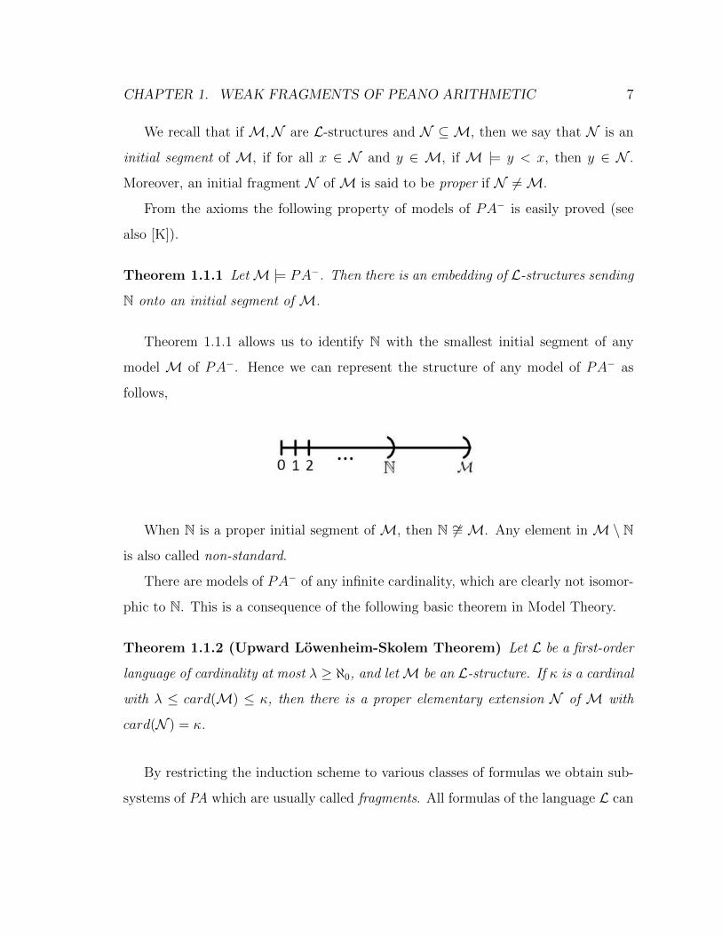
Theorem 1.1.1 allows us to identify N with the smallest initial segment of any

model M of PA−. Hence we can represent the structure of any model of PA− as

follows,

When N is a proper initial segment of M, then N 6∼=M. Any element in M\ N

is also called non-standard.

There are models of PA− of any infinite cardinality, which are clearly not isomor-

phic to N. This is a consequence of the following basic theorem in Model Theory.

Theorem 1.1.2 (Upward Lowenheim-Skolem Theorem) Let L be a first-order

language of cardinality at most λ ≥ ℵ0, and letM be an L-structure. If κ is a cardinal

with λ ≤ card(M) ≤ κ, then there is a proper elementary extension N of M with

card(N ) = κ.

By restricting the induction scheme to various classes of formulas we obtain sub-

systems of PA which are usually called fragments. All formulas of the language L can


be arranged in the following classes, of different complexity:

E0 = U0 = ∃0 = ∀0 = φ(x) : φ is quantifier-free,

∃n+1 = ∃y φ(x, y) : φ ∈ ∀n,

∀n+1 = ∀y φ(x, y) : φ ∈ ∃n,

En+1 = ∃y ≤ t(x) φ(x, y) : φ ∈ Un, t a term of L,

Un+1 = ∀y ≤ t(x) φ(x, y) : φ ∈ En, t a term of L,

∆0 = Σ0 = Π0 =⋃

n∈NEn =⋃

n∈N Un,

Σn+1 = ∃y φ(x, y) : φ ∈ Πn,

Πn+1 = ∀y φ(x, y) : φ ∈ Σn.

If C is any of the classes of formulas ∆0, Un, En,Πn,Σn,∀n,∃n, and we restrict

induction to be applied only on to C, we get the weak fragment of PA which is

denoted by IC. In particular, the weakest of these fragments of PA is the theory of

IE0, or Open Induction (also denoted by IOpen), where induction is only allowed on

open formulas (i.e. formulas with no quantifiers).

The systems described above have different mathematical strength as we increase

the complexity of formulas we are considering. The relation among these systems is

the following:

IOpen ⊂ IE1 ⊆ IE2 ⊆ · · · ⊆ I∆0 ⊂ IΣ1 ⊂ IΣ2 ⊂ · · · ⊂ PA.

Notice that the symbol ⊂ in the previous sequence denotes that the inclusion

between theories has been proved to be strict, while the symbol ⊆ means that it is

still unknown whether the inclusion is strict or not.

We already remarked that the set N of natural numbers is the standard model

of PA− and all fragments IC. Moreover, there is a very intuitive correspondence

between models of PA− and discretely ordered rings, which is the same as between Z

and N. Suppose M |= PA− and consider the following relation ”∼” on M2

(a, b) ∼ (c, d)⇔ a+ d = b+ c.


It is easy to verify that this is an equivalence relation, so we can consider R =M2/ ∼

and denote the equivalence class of (a, b) by [a, b]. Then if we define the following

operations and relation on R

[a, b] + [c, d] = [a+ c, b+ d],

[a, b] · [c, d] = [ac+ bd, bc+ ad],

[a, b] < [c, d]⇔ a+ d < b+ c,

and interpret 0 and 1 in R by [0, 0] and [1, 0] respectively, we obtain a discretely

ordered ring. The original structure M is then embedded in this ring via the map

a 7→ [a, 0], sending M onto the set of non-negative elements of R.

Conversely, if R is a discretely ordered ring and we denote the subset of non-

negative elements of R by M, then M is a model of PA−, from which the original

ring R is again obtained if we repeat the construction described above.

Henceforth in what follows, when no confusion arises, we will make no distinction

between a modelM of PA (or of any fragment IC) and its associated ring. When we

work with the ring, the axiom scheme of induction is clearly intended to be applied

to the non-negative part of the ring.

The main interests in these weaker systems lie mainly in the connection these

theories have with complexity theory, where number theory plays a central role. Many

open problems in theories such as I∆0 or I∆0 + Ω1 (which will be described later)

have complexity-theoretic counterparts.

For example, it is still an open problem if I∆0 proves the MRDP-theorem. This

theorem is due to Matijasevic, Robinson, Davis and Putnam and asserts that every

recursively enumerable set is existentially definable. Its proof led to the negative

solution of the well known Hilbert’s 10th problem. The MRDP-theorem can be re-

formulated in I∆0 as follows: for every Σ1-formula θ(x) there are polynomials p(x, y)

and q(x, y) such that

I∆0 ` ∀x (θ(x)↔ ∃y p(x, y) = q(x, y)) .


Wilkie (see [W]) observed that a proof of this theorem in I∆0 would give a positive

solution to the well known problem NP?= coNP . This follows from two considera-

tions.

(1) The set S = (a, b, c) ∈ N3 : ∃x < c∃y < c (ax2 + by = c) is NP -complete (see

[M-A]).

(2) If I∆0 `MRDP -theorem then ∆N0 = EN

1 , and this implies S ∈ NP∩co-NP.

It is also unknown if I∆0 + Ω1 proves MRDP -theorem and, again, a positive answer

would give NP = coNP .

1.2 Open Induction

As mentioned in the previous section, the weakest fragment of PA is the theory

Open Induction, denoted as IOpen, where induction is only allowed on formulas

without quantifiers. Models of this theory have been completely characterized (see [S]

and [Ot]) as follows:

Proposition 1.2.1 LetM be a discretely ordered ring. Then the following are equiv-

alent.

(1) M is a model of IOpen;

(2) every quantifier-free definable subset of M is a union of finitely many intervals

in M;

(3) for every r in Q(M) (the quotient field of M), there is a ∈ M such that

|a− r| < 1 and Q(M) is dense in RC(M), the real closure of M.

As a consequence it is possible to define the integer part [α] of any α ∈ RC(M)

in the usual way as

[α] = z ∈M⇔ z ≤ α < z + 1.


In models of IOpen it is also possible to perform Euclidean division and get, for

any x, y ∈M |= IOpen, y 6= 0, that x = qy + r for some q, r ∈M and 0 ≤ r < y.

Notice that in general models of IOpen lack the Euclidean algorithm for determin-

ing a greatest common divisor of any pair of elements ofM. This is a consequence of

the fact that in Bezout rings the notions of prime and irreducible elements coincide,

and this is not the case in models of IOpen, as it is shown in [M-M].

Of course, any model of PA, such as N, is also a model of IOpen, but this also

admits some ”pathological” models. There are models of IOpen where the equation

x2 = 2y2 admits non-trivial solutions (see [S]), hence IOpen does not prove irrational-

ity of√

2. Moreover, there are models of IOpen where the equation xn + yn = zn

admits non-trivial solutions for any natural number n, making Fermat’s Last Theorem

false in IOpen.

1.3 Bounded Induction

The theory we are mainly interested in is the fragment of PA denoted by I∆0,

where induction is allowed only on ∆0-formulas, i.e. formulas in which all quantifiers

are bounded by terms of the language. Hence a typical ∆0 statement has the form

∀x < t(x, a) φ(x, a),

for a formula φ(x, y), a term t(x, y) of the language L, and a n-tuple of parameters a.

Notice that in the language of arithmetic we are using, terms are actually polynomials.

When working in I∆0 care must be taken in expressing properties via ∆0-formulas,

since these are the only formulas we can induct on.

For example, we can express in a ∆0-way the following property:

x divides y : δ(x, y) = ∃z ≤ y (xz = y); (1.1)

and by ∆0-induction we can prove that, for every a, b

∃d ≤ a ∃x < b ∃y < a (δ(d, a) ∧ δ(d, b) ∧ d = ax+ by).


This implies that any two elements in any model of I∆0 have a greatest common

divisor, and thus all models of I∆0 are Bezout rings. This is enough to state that the

following strict inclusion holds:

IOpen ⊂ I∆0. (1.2)

We also remark that in the theory I∆0 induction can be used to prove that any

non empty set which is ∆0-definable has a minimum element. This will be used in

some proofs later.

One of the few known methods of getting models of bounded induction is by taking

particular initial segments of a model M.

Theorem 1.3.1 Let M |= I∆0 and let I be an initial segment of M. If I is closed

under + and · then I |= I∆0.

As an example, if M |= I∆0 and a ∈M, then the set

BP (a) = x ∈M : x < an, n ∈ N

is an initial segment closed under sum and multiplication, and so BP (a) |= I∆0.

A fundamental result for the theory I∆0 is due to Parikh (see [Pa]) and it is stated

in the following theorem.

Theorem 1.3.2 Let θ(x, y) be a ∆0-formula in the language L. If I∆0 ` ∀x∃y θ(x, y),

then I∆0 ` ∀x∃y < t(x) θ(x, y), where t(x) is a term of L.

Note that the theorem implies that if a function is ∆0-definable and provably total

in I∆0, then the function has polynomial growth.

This is the main limitation of I∆0. For example the classical result on the unbound-

edness of primes is proved using the function y =∏

p≤x p, where p is a prime. This

function is expressed by the ∆0-formula

∀p ≤ x (Pr(p)→ (δ(p, y) ∧ ¬δ(p2, x) ∧ ∀p ≤ y ((Pr(p) ∧ x < p)→ ¬δ(p, y)))),


where δ(x, y) is the ∆0-formula for divisibility (1.1), and Pr(p) is the ∆0-formula

standing for ”p is a prime”, namely

Pr(x) = ∀y ≤ x (δ(y, x)→ (y = 1 ∨ y = x)). (1.3)

The function y =∏

p≤x p is of exponential growth, so it is not provably total in I∆0.

As a consequence, it is still an open problem whether I∆0 proves cofinality of primes

or not.

If the axiom

exp : ∀x∃y (y = 2x)

is added to the theory, to guarantee the totality of the exponential function, then in

the theory I∆0 + exp cofinality of primes can be proved.

Notice that it is necessary to give a meaning to the function y = 2x in I∆0. This

is possible using a ∆0-formula defining exponentiation, which is due to Paris (see [G-

D]) which will be denoted by E0(x, y, z), where E0(x, y, z) denotes ”xy = z”. For

any n ∈ N, I∆0 6` ∀y∃z E0(n, y, z), hence the function defined by E0(x, y, z) is not

total in I∆0. But I∆0 proves the following algebraic properties for those elements on

which the function is defined.

(i) ∀x ≥ 1∀y∀z1∀z2 (E0(x, y, z1) ∧ E0(x, y, z2)→ z1 = z2)

(ii) ∀x ≥ 1∀y1∀y2∀z1∀z2 ((E0(x, y1, z1) ∧ E0(x, y2, z2)→ E0(x, y1 + y2, z1z2))

(iii) ∀x ≥ 1∀y1∀y2∀z1∀z2 ((E0(x, y1, z1) ∧ E0(z1, y2, z2)→ E0(x, y1y2, z2))

(iv) ∀x1 ≥ 1∀x2 ≥ 1∀y∀z1∀z2 (E0(x1, y, z1) ∧ E0(x2, y, z2) ∧ z1 < z2 → x1 < x2)

(v) ∀x ≥ 1∀y1∀y2∀z1∀z2 (E0(x, y1, z1) ∧ E0(x, y2, z2) ∧ y1 < y2 → z1 < z2).

Moreover, E0(x, y, z) satisfies the recursion lows for any x > 1 on which it is

defined, i.e.

(1) E0(x, 0, 1)


(2) ∀y∀z (E0(x, y, z)→ E0(x, y + 1, xz))

(3) ∀y∀z (E0(x, y + 1, z)→ ∃w < z (E0(x, y, w) ∧ z = wx)).

It can be proved that any other ∆0-formula satisfying (1), (2) and (3) is equivalent

to E0(x, y, z) in I∆0. Hence Paris’ formula gives an invariant meaning to the notion of

exponentiation in I∆0. So the axiom exp stating the totality of exponential function

2x can actually be expressed as exp : ∀x∃y E0(2, x, y).

The theory I∆0 + exp is strong enough to reproduce cofinality of primes, as well

as almost all the results from elementary number theory. In this theory it is usually

enough to adapt classical number-theoretical arguments and proofs, so no additional

constructive information arise.

On the contrary, many classical results do not hold in the theory I∆0. What is

available instead is factorization in powers of primes of any element. In order to see

this we use some lemmas.

Lemma 1.3.3 Let A be a bounded and ∆0-definable subset of M |= I∆0. Then A

has a maximum element.

Proof. Let φ(x) be the ∆0 formula defining the set A, and let α ∈M be an upper

bound for A.

The set X = y ≤ α : ∃t ≤ α (φ(t) ∧ y < t) is clearly ∆0-definable, and so is the

set Xc = M \ X = y : y > α ∪ y : y ≤ α ∧ ∀t ≤ α(φ(t) → y > t). Let

x0 = min(Xc); then x0 − 1 ∈ X, hence there is t ∈ A such that x0 − 1 ≤ t. But now

necessarily x0 − 1 = t, so x0 − 1 = max(A).

Lemma 1.3.4 Let A be a bounded, ∆0-definable subset of M |= I∆0. If there is a

non-zero m ∈ M divisible by all a ∈ A, then there is a non-zero µ ∈ M which is

minimal with respect to this property (i.e. if x ∈M is divisible by all elements of A,

then µ divides x).


Proof. Let φ(x) be the ∆0-formula defining the set A.

The set D = b : b 6= 0 ∧ ∀a ≤ m (φ(a) → δ(a, b)) is ∆0-definable and nonempty

since m ∈ D (here δ(a, b) is the usual ∆0-formula for divisibility (1.1)).

Let µ be the minimum of D. Now let x ∈M be divisible by all elements of A and

not by µ, then we have x = µq + r for q, r ∈ M, with 0 ≤ r < µ. Hence r = x− µq

is divisible by all elements of A, and since µ = min(D), it must be r = 0 and so µ

divides x.

The minimal element µ divisible by all elements of A will be called the least

common multiple of A and it will be denoted by lcm(A).

We also prove, by an easy ∆0-induction, that every element is divisible by a prime.

Lemma 1.3.5 I∆0 ` ∀x > 1 ∃p ≤ x (Pr(p) ∧ δ(p, x)).

Proof. Here Pr(p) is again the ∆0-statement for primes (1.3).

Let ψ(x) = ∀y ≤ x ∃p ≤ y (Pr(p)∧ δ(p, y)); clearly I∆0 ` ψ(2). Suppose I∆0 ` ψ(x)

and consider x+ 1. If x+ 1 is a prime, then I∆0 ` ψ(x+ 1). If x+ 1 is not a prime,

then there is a 1 < y ≤ x that divides x + 1. But from I∆0 ` ψ(x) we deduce that

there is a prime dividing y, and thus dividing x+ 1, hence I∆0 ` ψ(x+ 1).

We can express that an element is a power of a prime p with the ∆0-formula

Powp(x) = Pr(p) ∧ ∀y ≤ x (δ(y, x)→ δ(p, y)). (1.4)

This allows us to identify the greatest power of a prime that divides a given element.

Lemma 1.3.6 I∆0 ` ∀x > 1 ∀p (Pr(p)→ ∃!y ≤ x (Powp(y) ∧ δ(y, x) ∧ ¬δ(py, x))

Proof. Let M |= I∆0, x, p ∈M, with x > 1 and p a prime.

The set Axp = y : Powp(y) ∧ δ(y, x) of all powers of p dividing x is clearly ∆0-

definable and bounded by x, hence by Lemma 1.3.3 it has a maximum element.


We can now express that ”y is the greatest power of p that divides x” with the

∆0-formula

MPowp(x, y) = Powp(y) ∧ δ(y, x) ∧ ∀z ≤ x (Powp(z) ∧ δ(z, x))→ δ(z, y) (1.5)

For any x ∈M |= I∆0 we can consider the ∆0-definable set

Ax = y : ∃p ≤ x (Pr(p) ∧MPowp(x, y)) (1.6)

of all maximum powers of primes dividing x. Since x ∈ M is clearly divisible by

all elements of Ax, by Lemma 1.3.4 there is the smallest µ divisible by all elements

of Ax, which is trivially shown to coincide with x. Hence we have the property of

factorization in powers of primes for every element x of a model of I∆0 as the lcm(Ax).

What will also be used later is the following I∆0-version of the Chinese Reminder

Theorem (CRT).

Theorem 1.3.7 Let A be a bounded, ∆0-definable subset of M |= I∆0. Let f, r :

A −→ M be a ∆0-definable functions such that (f(a), f(b)) = 1 for every a, b ∈ M

and r(a) < f(a) for every a ∈ M. Suppose there is w ∈ M which is divisible by all

elements of f(A).

Then there is u <∏

a∈A f(a) such that u ≡ r(a)(mod f(a)) for every a ∈ A.

Proof. With∏

a∈A f(a) we mean the lcm(f(A)), which exists by Lemma 1.3.4

thanks to the hypothesis that there is w ∈ M which is divisible by all elements of

f(A).

First of all we remark that we can express the congruence ”x is equivalent to y

modulo z” via the ∆0-formula:

x ≡ y(mod z) : ∃k ≤ x (x = y + kz). (1.7)

Now let φ(x) be the ∆0 formula defining the set A, and consider the ∆0-formula

θ(x,w) = ∃u ≤ w

(u <

∏a∈A,a≤x

f(a) ∧ ∀t ≤ x (φ(t)→ u ≡ r(t)(mod f(t)))

).


By ∆0-induction we show that M |= ∀x (φ(x)→ θ(x,w)).

Clearly M |= (φ(1) → θ(1, w)) (it is equivalent to state that a solution to one

congruence always exists).

Now suppose M |= (φ(x)→ θ(x,w)) for an x ∈ M, and let u∗ <∏

a∈A,a≤x f(a) and

u∗ ≡ r(a)(mod f(a)) for all a ∈ A, a ≤ x. Now, supposing x + 1 ∈ A, the following

system of two congruencesu ≡ u∗(mod

∏a∈A,a≤x f(a)

)u ≡ r(x+ 1)(mod f(x+ 1))

(1.8)

has a solution since the moduli are relatively prime by hypothesis (if we put α =∏a∈A,a≤x f(a), since (α, f(x + 1)) = 1 we know that there are h, k ∈ M such that

hα + kf(x + 1) = 1; then u = u∗kf(x + 1) + r(x + 1)hα is a solution to the system

(1.8)). Hence M |= (φ(x+ 1)→ θ(x+ 1, w)).

We remark that the previous statement is a generalization of the classic CRT

where A = m1, . . . ,mk ⊆ Z is a finite set of pairwise relatively prime moduli,

ri < mi for all i = 1, . . . , k and we are looking for integer solutions of the set of

congruences x ≡ r1(mod m1)

...

x ≡ rk(mod mk)

.

1.4 Pigeonhole principle and Ω1

Even though the theory I∆0 is strong enough to prove factorization of elements as

products of primes, there are many other classical number-theoretical results whose

provability in I∆0 are still open problems. The main obstacle in obtaining results

like unboundedness of primes is, as we mentioned before, the lack of functions of


exponential growth rate, such as factorials, since they are not provably total in models

of I∆0.

An important result is due to Woods (see [Wo]), who proved that in some cases

such functions can be avoided and replaced by combinatorial principles such as the

Pigeonhole Principle. He showed that if we add to the theory I∆0 the following

∆0-version of the pigeonhole principle (∆0-PHP)

∀x < z ∃y < z θ(x, y)→ ∃x1 < z + 1 ∃x2 < z + 1 (x1 6= x2 ∧ θ(x1, y) ∧ θ(x2)),

where θ(x, y) runs through all ∆0-formulas, the resulting theory I∆0 + ∆0-PHP is

strong enough to prove the existence of arbitrarily large primes.

Notice that ∆0-PHP actually is an axiom scheme, and it basically says that there

is no injective ∆0-function from z + 1 into z, and we can also use the notation

¬∃z F : z + 1 z.

What Woods actually proved is then the following.

Theorem 1.4.1 I∆0 + ∆0-PHP ` ∀x∃p (Pr(p) ∧ p > x).

Paris, Wilkie and Woods [P-W-W] later improved this result showing that in order

to prove unboundedness of primes in I∆0 a weaker version of the PHP is sufficient.

This principle, that will be denoted by ∆0-WPHP (weak pigeonhole principle), asserts

that there is no injective ∆0-function from (1 + ε)z into z, for every rational number

ε such that the integer part of (1 + ε)z is greater than z. This latter result is hence

as follows.

Theorem 1.4.2 I∆0 + ∆0-WPHP ` ∀x∃p (Pr(p) ∧ p > x).

The weak pigeonhole principle is provable (as it is showed in [P-W-W]) in the

theory I∆0 + Ω1, where Ω1 is the axiom

∀x∀y∃z(xlog2y = z

). (1.9)


Notice that the quantity log2y here has a ∆0-meaning, as the following lemma

guarantees.

Lemma 1.4.3 Let M |= I∆0 and let a,m ∈ M, with m > 0, a > 1. Then there is

a unique l0 ∈M such that al0 ≤ m < al0+1.

Proof. Here we use the ∆0 we have mentioned before.

The set A = l ∈ M : ∃b ≤ m E0(a, l, b) is clearly ∆0-definable in M, and it is

bounded and non-empty. Hence, by Lemma 1.3.3, it has a maximum element l0, so

it is al0 ≤ m < al0+1.

Consider the formula

λ(x, y, z) = ∃w ≤ x (E0(y, z, w) ∧ w ≤ x ∧ x < wy) .

By the previous lemma for every a,m ∈ M, with m > 0, a > 1 there is a unique l0

such thatM |= λ(m, a, l0); so the formula λ(x, y, z) extends the meaning of ”z is the

(unique) logarithm of x in basis y” toM. So we can express the axiom Ω1 introduced

before as

∀x∀y∃z (∃t ≤ y (λ(y, 2, t) ∧ E0(x, t, z))).

The theory I∆0+Ω1 has been widely studied and much is known about its number-

theoretical strength. We already mentioned that in [P-W-W] cofinality of primes is

proved in I∆0 + Ω1 (which is still an open question in I∆0) and the weak version of

the pigeon-hole principle ∆0-WPHP. Notice that, even though function of exponential

growth are still ”out of range” in I∆0+Ω1, the axiom Ω1 increases the strength of the

theory I∆0, allowing us to consider functions of growing rate more than polynomial,

thanks to the totality of the function xlog2y. Hence we can state that

I∆0 ⊂ I∆0 + Ω1. (1.10)

Moreover I∆0 + Ω1 also proves many classical results like Lagrange’s four squares

theorem (see [B-I]) and basic results about residue fields (see [D-M]).


Anyway the theory I∆0 +Ω1 is strictly weaker than I∆0 +exp: letM be a model

of I∆0 + Ω1 and a ∈M be non-standard (i.e. a ∈M \ N); if we consider the set

BL(a) =x ∈M : x < a(log2a)

n

for some n ∈ N

we have that BL(a) |= I∆0 + Ω1, but BL(a) 6|= exp. Thus we have I∆0 + Ω1 6` exp,

and recalling the previous relations (1.2) and (1.10), the following chain of strict

inclusions holds for the weak fragments of PA we have described:

IOpen ⊂ I∆0 ⊂ I∆0 + Ω1 ⊂ I∆0 + exp.

Chapter 2

Legendre’s theorem

In this chapter we are going to show a proof of Legendre’s theorem in the theory

I∆0 + Ω1. In order to do this we will provide all necessary tools and, even though

the final proof of the theorem requires the axiom Ω1, all properties will be stated and

proved in the weakest possible fragment of PA that makes them valid, i.e. I∆0.

2.1 Legendre’s theorem and its equivalent

Legendre’s theorem gives a necessary and sufficient condition for the existence

of non trivial solution for certain quadratic equations with integer coefficients. The

equations considered are of the form

ax2 + by2 + cz2 = 0, (2.1)

with a, b, c ∈ Z \ 0, square free, relatively prime and, clearly, not all of the same

sign. For a non trivial solution we mean a solution (x0, y0, z0) ∈ Z different from

(0, 0, 0).

An integer a is square free if no square divides a, or equivalently all primes dividing

a appear in with exponent 1 the factorization of a. We remark that this property is

∆0-definable via the formula:

σ(x) = ∀y ≤ x (Pr(y)→ ¬δ(y2, x)),

21

CHAPTER 2. LEGENDRE’S THEOREM 22

where δ(y, x) =”y divides x” and Pr(y) =”y is a prime” are expressed by the ∆0-

formulas (see also 1.1) and (1.2):

δ(y, x) = ∃z ≤ x (yz = x)

Pr(y) = ∀x ≤ y (δ(x, y)→ (x = 1 ∨ y = x)).

We will consider congruences in I∆0: as for the classical definition on integers we

say that a is congruent to b modulo c, with a, b, c ∈ M |= I∆0, c 6= 0, if c divides

b− a, and this can be expressed by the ∆0-formula

γ(a, b, c) = ∃m ≤ a (a = mc+ b). (2.2)

We will also denote this fact as a ≡ b(mod c). Given any a, c ∈ M, c 6= 0, we can

always consider some b ∈M such that a ≡ b(mod c) and |b| ≤ c/2. This follows from

the fact that we can find q, r ∈ M such that a = qc + r, with 0 ≤ r < c, and so we

have a ≡ r ≡ r − c(mod c), with either r or r − c ≤ c/2.

Moreover, we will use the fact that if two elements a and b are relatively prime,

a is invertible modulo b, and viceversa. Recall that models of I∆0 are Bezout rings,

so if (a, b) = 1 then there are h, k such that ah + bk = 1, so ah ≡ 1(mod b), and

we can identify a−1 with h. This is a ∆0-property since it can be expressed by the

∆0-formula

Inv(a, b) = ∃w ≤ b γ(aw, 1, b), (2.3)

where γ is the ∆0-formula for congruences (2.2).

We will denote the fact that a is a square modulo b by aRb. This is ∆0-definable

via:

ρ(a, b) = ∃x ≤ b/2 ∧ ∃m ≤ a(a = x2 +mb).

We now fix a modelM of I∆0 + Ω1. The statement of Legendre’s theorem inM

is as follows.

Theorem 2.1.1 (Legendre) Let a, b, c ∈ M \ 0 be non-zero, not all of the same

sign, square-free and pairwise relatively prime. Then the equation

ax2 + by2 + cz2 = 0


has a non trivial solution in M if and only if

(Leg.1) −abRc,

(Leg.2) −bcRa,

(Leg.3) −acRb.

Remarks:

1. If a non trivial solution (x0, y0, z0) of (2.1) exists, then we can consider x0, y0, z0

to be pairwise relatively prime (and call such a solution primitive). Indeed, suppose

p is a prime and p divides x0 and y0. Then p2|cz20 , and since c is square free, p|z20 and

so p|z0, so we can factor out p and consider the solution (x0/p, y0/p, z0/p).

2. The necessary condition of Theorem 2.1.1 is easily proved, even in models of

I∆0:

Proof. (=⇒ of 2.1.1) Let (x0, y0, z0) be a primitive solution of (2.1) in a modelM

of I∆0. Then

ax20 + by20 + cz20 = 0, (2.4)

and reducing modulo a we get −by20 ≡ cz20(mod a).

Now if a prime p divides a and y0, equation (2.4) implies that p|cz20 . From (a, c) = 1

we get that p 6 |c and so p|z0. Hence p divides y0 and z0, which is a contradiction.

Hence we have (a, y0) = 1, and y0 is invertible modulo a. So we can write −b ≡

cz20(y−10 )2(mod a), where y−10 is given by the formula Inv(y0, a) (see (2.3)). Hence

we can rewrite −bc ≡ (cz0y−10 )2(mod a), i.e. −bcRa. In the same way, being the

equation (2.1) symmetric for a, b and c, we also get −abRc and −acRb.

In order to prove Legendre’s theorem in any model of I∆0 + Ω1, we consider the

following equivalent normal form. Using the same notation as before, the statement

is as follows.


Theorem 2.1.2 (Legendre normal form) Let a, b ∈ M \ 0 be square-free and

positive. Then the equation

ax2 + by2 = z2 (2.5)


(Norm.1) aRb,

(Norm.2) bRa,

(Norm.3) − abd2Rd, where d = (a, b).

Remarks:

1. Using the same arguments as before we can assume that, if a non trivial

solution (x0, y0, z0) of the equation (2.5) exists, it is primitive (i.e. x0, y0, z0 pairwise

relatively coprime).

2. The necessary condition of the Theorem 2.1.2 is proved as follows, in any model

of I∆0.

Proof. (=⇒ of 2.1.2) Let (x0, y0, z0) be a primitive solution of (2.5) in a modelM

of I∆0, i.e.

ax20 + by20 = z20 . (2.6)

We have (a, y0) = 1. Indeed, if p is a prime and p divides a and y0, then p|z20 , and

sop|z0. Then we get p|(y0, z0), contradicting the fact that the solution is primitive.

So y0 is invertible modulo a in M, and we have by20 ≡ z20(mod a), which implies

b ≡ (z0y−10 )2(mod a), i.e. bRa.

Similarly, by symmetry of the equation (2.6) on the coefficients a and b, we can

show that aRb.

In order to obtain condition (Norm.3) of the theorem, we first observe that d is

square-free since a, b are. Moreover, if a = da′ and b = db′, with (a′, b′) = 1, from

(2.6) we get

d(a′x20 + b′y20) = z20 , (2.7)


i.e.d|z20 . Since d is square-free d divides z0. Let z0 = dz′0.

From (2.7) we have:

a′x20 + b′y20 = z20/d = (dz′0)2/d = d(z′0)

2 (2.8)

which can be rewritten asa

dx20 +

b

dy20 = d

(z0d

)2. (2.9)

Hence −adx20 = b

dy20 − d

(z0d

)2 ≡ bdy20(mod d).

We already noticed that (x0, b) = 1, so also (x0, d) = 1, hence x0 is invertible

modulo d. So we have

−ad≡ b

dy20(x−10 )2(mod d)⇒ −a

d

b

d≡(b

dy0x

−10

)2

(mod d),

that means − abd2Rd.

The next step is to prove the equivalence between the two statements of Legendre’s

theorem. We will use the following lemma.

Lemma 2.1.3 Let a,m, n ∈ M |= I∆0, m,n relatively prime. If aRm and aRn,

then aRmn.

Proof. From the hypothesis there are α, β ∈M, α ≤ m/2, β ≤ n/2 such that

a ≡ α2(mod m) and b ≡ β2(mod n).

Consider the system of congruencesx ≡ α(mod m)

x ≡ β(mod n)

. (2.10)

Since (m,n) = 1, the system (2.10) has a solution γ ∈M by Theorem 1.3.7 (∆0-CRT)

. Hence, we have

γ ≡ α(mod m) and γ ≡ β(mod n).


Then we have

a ≡ γ2(mod m) and a ≡ γ2(mod n),

that means that both m,n divide a − γ2. Since m,n are relatively prime, we have

that mn divides a− γ2, that means a ≡ γ2(mod mn), i.e. aRmn.

We can now prove the following theorem.

Theorem 2.1.4 Theorems 2.1.1 and 2.1.2 are equivalent.

Proof. (2.1.1 =⇒ 2.1.2) To prove this implication we assume Theorem 2.1.1 valid,

and we only have to prove the sufficient condition [⇐=] of Theorem 2.1.2, since the

other implication has already been shown to be true.

So we consider an equation

ax2 + by2 = z2, (2.11)

with a, b ∈M |= I∆0, a, b square-free and positive, and suppose conditions

(Norm.1) aRb,

(Norm.2) bRa,

(Norm.3) − abd2Rd, where d = (a, b)

of Ttheorem 2.1.2 hold.

We now consider the equation

a

dx2 +

b

dy2 + (−d)z2 = 0, (2.12)

which can be written as

Ax2 +By2 + Cz2 = 0, (2.13)

where A = ad, B = b

dand C = −d.

The coefficients A,B,C are square-free and pairwise relatively prime. We have:

−AB = −abd2

, and we know that − ab

d2Rd by (Norm.3),


hence we have −ABRC. Moreover,

−AC = −ad

(−d) = a, and we know that aRb by (Norm.3), so aR bd,

that means −ACRB. Finally,

−BC = − bd

(−d) = b, and bRa by (Norm.2),

which implies bRad, that means −BCRA.

So the three conditions of Theorem 2.1.1 hold for the equation (2.12). We can

deduce that equation (2.12) has a non trivial solution (x0, y0, z0), i.e.

a

dx20 +

b

dy20 + (−d)z20 = 0

which implies ax20+by20 = (dz0)2. Hence the triple (x0, y0, dz0) is a non-trivial solution

of (2.11).

(2.1.2 =⇒ 2.1.1) As before, to prove this implication we assume Theorem 2.1.2

valid, and we prove the sufficient condition [⇐=] of Theorem 2.1.1.

Consider the equation

ax2 + by2 + cz2 = 0, (2.14)

with a, b, c ∈M |= I∆0, a, b, c square-free, pairwise relatively prime and not all of the

same sign. W.l.o.g. we can assume a, b > 0 and c < 0, and suppose the conditions

(Leg.1) −abRc,

(Leg.2) −bcRa,

(Leg.3) −acRb

of Theorem 2.1.1 hold.

If we multiply both sides of (2.14) by −c we obtain the equation

(−ac)x2 + (−bc)y2 = (cz)2, (2.15)


which can be written as

Ax2 +By2 = Z2, (2.16)

where A = −ac,B = −bc and Z = cz.

Here the coefficients A and B are square-free (since a, b, c are pairwise relatively

prime) and positive.

From (Leg.3) we have ARb, and also ARc since c|A, and since (b, c) = 1 we can

apply Lemma 2.1.3 to obtain that ARB. In the same way we can prove that BRA.

Finally, notice that (A,B) = (ac, bc) = c, and

−ABc2

= 1−(ac)(−bc)

c2= −ab, and we know that − abRc from (Leg.1),

hence we have −ABc2Rc. We can conclude that all conditions of Theorem 2.1.2 hold

for the equation (2.16), so it has a non trivial solution (x0, y0, Z0), for which Z0 = cz0,

for some z0 ∈M, and

(−ac)x20 + (−bc)y20 = (cz0)2 ⇐⇒ c(−ax20 − by20) = c2z20 ⇐⇒ ax20 + by20 = cz20 ,

hence (x0, y0, z0) is a non-trivial solution of (2.14).

2.2 Proof of the theorem in I∆0 + Ω1

In this section we are going to prove Legendre’s theorem in the theory I∆0 + Ω1 by

proving its equivalent normal form. The proof follows the main ideas of that in [I-R].

We will pay close attention in adapting all the arguments in I∆0 + Ω1.

We start from the following lemmas which imply a crucial result that will be used

in the main proof.

Lemma 2.2.1 If p ∈M |= I∆0 is a prime and −1 is a square modulo p (i.e. −1Rp),

then there is k ∈M, with k < p, such that kp = 1 + a2, for a ≤ p−12

.

Proof. Let a ∈M, a ≤ p−12

be such that −1 ≡ a2(mod p). This means that there

is k ∈M such that

kp = a2 + 1 ≤(p− 1

2

)2

+ 1.


We can prove that(p−12

)2+ 1 < p2. Indeed, if not, we would get p2 + 2p − 3 ≤ 0,

which implies −3 ≤ p ≤ 1, a contradiction.

Hence we have kp < p2, with k < p, and kp = 1 + a2.

Lemma 2.2.2 Let p ∈ M |= I∆0 be a prime. If there is k ∈ M, with k < p such

that kp is the sum of two squares, then p itself is the sum of two squares.

Proof. It is clear that 2 = 1 + 1 is a sum of two squares, so we can assume p 6= 2.

The set S(p) = m ∈M : m < p and mp is the sum of two squares , is ∆0-definable

via the formula σ(x) = ∃y < p ∃z < p (xp = y2 + z2), and it is clearly bounded by p

and, by hypothesis, not empty. By ∆0-induction S(p) has a minimum element, and

we now show that it is 1.

Let h ∈ M be the minimum of S(p), and let , a, b < p be such that hp = a2 + b2.

Suppose that h > 1, and we show that we can find a h′ ∈ S(p) with h′ < h. We will

distinguish two cases.

• case h is even: then a and b must be both even or both odd.

If a, b are both even we can write

hp = 4

((a2

)2+

(b

2

)2),

hence 4 divides h and we have

h

4p =

(a2

)2+

(b

2

)2

.

So there is h′ = h/4 < h and h′p is the sum of two squares.

If a, b are both odd we can write

h

2p =

(a− b

2

)2

+

(a+ b

2

)2

,

so again we get h′p as a sum of two squares, with h′ = h/2 < h.

• case h is odd: let a ≡ α(mod h) and b ≡ β(mod h), with α, β < h2. Then

hp = a2 + b2 ≡ α2 + β2 ≡ 0(mod h),


hence there is j ∈M such that

α2 + β2 = jh, (2.17)

and j < h since α2 + β2 < (h/2)2 + (h/2)2 = h2/2 < h2.

Now from a2 + b2 = kp and (2.17) we obtain

(a2 + b2

) (α2 + β2

)= jh2p. (2.18)

Since (a2 + b2

) (α2 + β2

)= (aα + bβ)2 + (aβ − bα)2 ,

and aα+ bβ ≡ α2 + β2 ≡ 0(mod h), we have that h divides aα+ bβ and, similarly, h

divides aβ − bα.

Henceforth, from (2.18) we obtain(aα + bβ

h

)2

+

(aβ − bα

h

)2

= jp,

so we have jp as a sum of two squares and j < h.

It is now easy to deduce the following property.

Proposition 2.2.3 Let M |= I∆0 and let p ∈ M be a prime. If −1 is a square

modulo p, then p is the sum of two squares.

Proof. It is sufficient to observe that if −1 is a square modulo p, then by Lemma 2.2.1

there are k, a ∈ M, k, a < p, such that kp = 1 + a2, which is clearly a sum of two

squares. The statement then follows straightforward from Lemma 2.2.2.

We now use the previous result to reproduce a property of the integers in models

of I∆0 + Ω1, that will be used later in the proof of Legendre’s theorem.

Proposition 2.2.4 Let M |= I∆0 and b ∈M. If −1 is a square modulo b, then b is

the sum of two squares.


Proof. If −1 is a square modulo b, then −1 is a square modulo every prime p dividing

b. Proposition 2.2.3 implies that every prime dividing b is the sum of two squares.

It is easy to verify that the product of sums of two squares is still a sum of two

squares (e.g. (a2+b2)(c2+d2) = (ac+bd)2+(ad−bc)2). We can iterate this argument

to the product of all primes dividing b, which is of logarithmic length with respect to

b (roughly log2 b), where all the partial products are bounded by b itself.

Remarks:

On most texts on classic number theory the previous properties are proved using

tools such as the (full) Pigeonhole Principle, which we have not available even in I∆0+

Ω1, or Legendre’s symbol(

ap

)(see [H-W]) and the property that

(ap

)= a

p−12 (mod p),

which is not known to be valid in I∆0. The arguments showed above is thus an

adaptation of classical results to our context.

We can now go through the proof of theorem 2.1.2 in the theory I∆0 + Ω1. In the

first part we show how to get a solution of the considered equation, and in the second

part we formalize its existence in I∆0 + Ω1. Here we restate the theorem.

Theorem 2.2.5 (Legendre normal form) Let M |= I∆0 + Ω1 and let a, b ∈ M

be square-free and positive. Then the equation

ax2 + by2 = z2 (2.19)


(Norm.1) aRb,

(Norm.2) bRa,

(Norm.3) − abd2Rd, where d = (a, b).

Proof. As noticed in the remarks following the statement of 2.1.2, we only have

to prove that the properties (Norm.1-3) imply that the equation (2.19) has a non-

trivial solution. Consider such an equation and suppose conditions (Norm.1-3) hold

for a, b ∈M, a, b square-free and positive. There are some trivial cases:


• Case a = 1: then (2.19) becomes x2+by2 = z2 and the triple (1, 0, 1) is a non-trivial

solution;

• Case b = 1: as before, being (0, 1, 1) a non-trivial solution for ax2 + y2 = z2;

• Case a = b: then (2.19) becomes b(x2 + y2) = z2, and the condition (Norm.3)

says that − b2

b2Rb, i.e. −1Rb; now, by proposition 2.2.4 we know that there are

r, s ∈ M such that b = r2 + ss, and the triple (r, s, b) represents a non-trivial

solution of the equation.

Notice that in all these trivial cases the solution (x0, y0, z0) is such that x0, y0, z0 ≤

a.

We can now consider a, b > 1 and, a 6= b; without loss of generality we suppose

b < a. The argument is as follows: from the starting equation (2.19) we build another

equation

Ax2 + by2 = z2, (2.20)

with 0 < A < a and satisfying the appropriate conditions (Norm.1-3), such that if

(2.20) has a non-trivial solution, we obtain a non-trivial solution of (2.19) from it.

By applying repeatedly this argument, possibly switching the role of the coefficients

a and b at some point, we eventually get to one of the trivial cases a = 1, b = 1 or

a = b, that admit a non-trivial solution, and going backward from that we obtain a

non-trivial solution to (2.19). We have to formalize this argument by ∆0 induction.

For the equation ax2 + by2 = z2 we know from (Norm.2) that there is β ≤ a/2

such that b ≡ β2(mod a), hence there is k ≤ a such that β2 − b = ka. If we factor

out the squares in k we can write

β2 − b = h2Aa, (2.21)

with A square-free. This is the coefficient we use in equation (2.20) we are going to

work with.


Now

0 ≤ β2 = h2Aa+ b < h2Aa+ a = a(h2A+ 1)⇒ h2A+ 1 > 0⇒ A > − 1

h2≥ −1,

hence A ≥ 0. On the other hand, if A = 0 then b = β2, a contradiction since b is

square-free. We have then proved that A > 0.

Moreover, from (2.21) we also get

aA ≤ aAh2 < β2 ≤ a2

4,

that means

A <a

4. (2.22)

This inequality will turn out to be very important later.

Now if d = (a, b) then a = da1, b = db1, with (a1, b1) = 1.

If a prime p divides both a1 and d, then p2 divides a, and since a is square-free we

have (a1, d) = 1, and the same argument shows (b1, d) = 1.

From (2.21) we get

β2 = h2Aa+ b = h2Aa1d+ b1d = d(h2Aa1 + b1),

hence d divides β2, and since d is square-free, we have d|β. Llet β = dβ1, then

β2 = d2β21 and we have d2β2

1 = d(h2Aa1 + b1), hence

dβ21 = h2Aa1 + b1. (2.23)

Now, if any prime p divides both d and h, from (2.23) it follows that p divides b1,

and hence p divides both b1 and d, a contradiction since they are relatively prime. So

necessarily (d, h) = 1. From (2.23) we obtain

h2Aa1 ≡ −b1(mod d) which implies h2Aa21 ≡ −b1a1(mod d),

and since (a1, d) = (h, d) = 1, both h and a1 are invertible modulo d. So we have

A ≡ −a1b1(h−1a−11

)2(mod d).


Now, since −a1b1 = − abd2

, condition (Norm.3) tells us that −a1b1 is a square modulo

d, and so we get

ARd. (2.24)

Notice that if there is a prime p which divides both h and b, then from (2.21) we get

that p divides β an then p2 divides b, and this is a contradiction since b is square-free.

Hence (h, b) = 1. Since b1 divides b, also (h, b1) = 1. Then from (2.21) the following

implication holds

h2Aa ≡ β2(mod b1)⇒ A ≡ β2(h−1)2a−1(mod b1).

From (Norm.1) states that aRb it follows that aRb1, and so

ARb1. (2.25)

Now from (2.24), (2.25) and Lemma 2.1.3 we get

ARb. (2.26)

Moreover, from (2.21) we know that b ≡ β2(mod A), that means

bRA. (2.27)

If r = (A, b), then it is left to show that −Abr2Rr.

Let A = A2r, b = b2r, with (A2, b2) = 1. We have (r, A2) = (r, b2) = 1 since A, b are

square-free. From (2.21) we obtain

β2 = b2r + h2A2ra = r(b2 + h2A2a). (2.28)

So r divides β2, and since r is square-free, we have r|β. Let β = β2r, from (2.28) we

get the following implications

rβ22 = b2 + h2A2a⇒ h2A2a ≡ −b2(mod r)⇒ −A2b2h

2a ≡ b22(mod r). (2.29)

Now using the same arguments as before we can show that (a, r) = (h, r) = 1, so

both a, h are invertible modulo r, and we obtain

−A2b2 ≡ b22(h−1)2a−1(mod r).


Recalling that aRb and r|b, we have that aRr, and since −A2b2 = −Abr2

, the previous

congruences imply that

−Abr2Rr. (2.30)

We have then obtained the equation (2.20) Ax2 + by2 = z2, with 0 < A < a/4, A

square-free and (by (2.26), (2.27) and (2.30)) satisfying the conditions

(Norm.1) ARb,

(Norm.2) bRA,

(Norm.3) −Abr2Rr, where r = (A, b).

The single reduction we have made can easily be formalized in I∆0, since it is

based only on congruences and the quantifiers are obviously bounded by the initial

coefficients a and b.

Now suppose (x0, y0, z0) is a non-trivial solution of (2.20), hence

Ax20 = z20 − by20 (2.31)

By multiplying (2.31) by (2.21) we have

A2x20h2a = (z20 − by20)(β2 − b) = z20β

2 − bz20 − by20β2 + b2y20;

if we now add and subtract the quantity 2z0βby0 we have

A2x20h2a = (z20β

2+b2y20+2z0βby0)−b(z20+y20β2+2z0βby0) = (z0β+by0)

2−b(z0+y0β)2,

and so

a(Ax0h)2 + b(z0 + y0β)2 = (z0β + by0)2,

which states that the triple

(Ax0h, z0 + y0β, z0β + by0)

is a non-trivial solution of equation (2.19).


We now need to estimate the growth rate of the solution of equation (2.19) in

terms of that of (2.20).

First of all, notice that if Ax20 + by20 = z20 , then clearly x0, y0 ≤ z0 (remember that

both A and b are positive).

Then, as already showed, the components of the solution of (2.19) are

• Ax0h ≤ xoa4

(since Ah < a4)

• z0 + y0β ≤ z0 + z0β = z0(1 + a

2

)(since β ≤ a

2)

• z0β + by0 ≤ z0a2

+ az0 = z0(32a)

and since we are assuming a > 1 we can conclude that all the components of the new

solution are ≤ z0(32a).

We now have to iterate this procedure and formalize it in I∆0 + Ω1. We start

with the given equation

E0 : ax2 + by2 = z2, (2.32)

where a, b are square-free, a > b and

aRb, bRa, −abd2Rd, where d = (a, b),

and we build a sequence of equations, for i > 0

Ei : Aix2 +Biy

2 = z2, (2.33)

where every Ai, Bi are defined by recursion as follows (where A0 = a,B0 = b)

• β2i −Bi = h2iAiAi−1, Bi = Bi−1 (2.34)

with Aihi <Ai−1

4, βi ≤ Ai−1

2, if at step i− 1 we have Ai−1 > Bi−1, or

• α2i − Ai = h2iBiBi−1, Ai = Ai−1 (2.35)

with Bihi <Bi−1

4, αi ≤ Bi−1

2, if at step i− 1 we have Ai−1 < Bi−1.


For every equation Ei the following congruence conditions hold.

AiRBi, BiRAi, −AiBi

r2iRri, where ri = (Ai, Bi).

Moreover, if (xi, yi, zi) is a non-trivial solution of equation Ei, then a non-trivial

solution of Ei−i is either

• (Aixihi, zi + yiβi, ziβi +Bi−1yi) (2.36)

or

• (zi + yiαi, Bixihi, ziαi + Ai−1yi) (2.37)

according to Ai−1 > Bi−1 or Ai−1 < Bi−1, respectively.

We remark that:

(i) the growth factor from a solution of the equation Ei to that of Ei−1 is always

bounded by 32Ai−1 ≤ 3

2a when Ai−1 > Bi−1, and by 3

2Bi−1 ≤ 3

2b when Ai−1 <

Bi−1;

(ii) when ”descending” through the sequence, the coefficients of equation Ei and

those of equation Ei−1 are related as follows:

Ai <Ai−1

4≤ a

4or Bi <

Bi−1

4≤ b

4.

Hence the length of the sequence of Ei’s is at most log4a+ log4b.

(iii) the sequence of equations will eventually stop with one of the trivial cases where

one of the coefficients is 1 or they are equal. In these cases non trivial solutions

exist, namely (1, 0, 1) or (0, 1, 1) or (ri, si, Bi), where Bi = r2i + s2i .

Let l be the length of the sequence. For the final solution of equation El we can

clearly state that xl, yl, zl ≤ b (where b is the coefficient of the initial equation (2.19)).

From remarks (i) and (ii) we can derive that all the components of the non-trivial

solution (x0, y0, z0) of E0, and so of (2.19), are bounded as follows

x0, y0, z0 ≤ b

(3

2a

)log4a(

3

2b

)log4b

. (2.38)


It is only left to formalize the recursion we have constructed in I∆0 + Ω1.

For the sake of clarity we will recall here all the ∆0-formulas we need:

• x divides y: δ(x, y) = ∃z ≤ y (xz = y)

• x is a prime: Pr(x) = ∀y ≤ x (δ(y, x)→ (y = 1 ∨ y = x))

• z is the g.c.d. of x and y:

γ(x, y, z) = δ(z, x) ∧ δ(z, y) ∧ ∀t ≤ x (δ(t, x) ∧ δ(t, y))→ δ(t, z)

• x is square-free: σ(x) = ∀y ≤ x (Pr(y)→ ¬δ(y2, x))

• x is a square modulo y: ρ(x, y) = ∃z ≤ x ∧ ∃r ≤ y/2 (x = r2 + zy).

We can now express all conditions of the theorem with a ∆0-formula:

Θ(a, b) = 0 ≤ a ∧ 0 ≤ b ∧ σ(a) ∧ σ(b) ∧ ρ(a, b) ∧ ρ(b, a)∧

∧ ∀d ≤ a

(γ(a, b, d)→ ρ

(−abd2, d

)).

(2.39)

We now make induction on the formula

Λ(t) = ∀a ≤ t ∀b ≤ t (ab ≤ t ∧ b ≤ a ∧Θ(a, b)) −→

∃x, y, z ≤ b

(3

2a

)log4a(

3

2b

)log4b

¬(x = 0∧ y = 0∧ z = 0)∧ (ax2 + by2 = z2), (2.40)

which is a ∆0 formula that uses boundaries which are allowed by the axiom Ω1.

For t = 1 the formula is true since in this case a = b = 1 and the equation

x2 + y2 = z2 has non-trivial solutions, for example (1, 0, 1), which clearly satisfy

x, y, z ≤ 1 ·(32· 1)log41 (3

2· 1)log41 = 1.

Now suppose M |= Λ(t), with t ∈M, t > 1, and consider t′ = t+ 1

Let a, b ∈ M, a, b ≤ t′; and ab = t′ (if ab < t′ ⇒ ab ≤ t and we already know Λ(t) is

true).

W.l.o.g. we can assume b < a, and hence apply the first step of the reduction and

obtain the equation Ax2 + by2 = z2, with A < a/4 and M |= Θ(A, b).


Now Ab < t′, hence Ab ≤ t, so by inductive hypothesis (M |= Λ(t)), this equation

admits a non-trivial solution (x1, y1, z1) in M, such that

x1, y1, z1 ≤ b

(3

2A

)log4A(

3

2b

)log4b

.

From this we showed how we can get a non-trivial solution (x0, y0, z0) of the

equation ax2 + by2 = z2, and by the previous observations we made we can state that

x0, y0, z0 ≤ b

(3

2A

)log4A(

3

2b

)log4b(

3

2a

)≤ b

(3

2a

)log4A+1(3

2b

)log4b

.

Since A < a/4, we have log4A ≤ log4a− 1, and we can conclude that

x0, y0, z0 ≤ b

(3

2a

)log4a(

3

2b

)log4b

.

Hence we have that M |= Λ(t′), and this concludes the proof.

Concluding remarks:

We have adapted a proof of Legendre’s theorem suggested in [I-R]. Cassels in [C]

obtained a linear bound of the solution in terms of the initial coefficients. Unfortu-

nately the proof uses tools of geometry of numbers which seem to rely on the (full)

pigeonhole principle, which is not known to be provable in I∆0+Ω1. Hence a possible

further development in this subject could be to search for an alternative proof with

no use of PHP , in order to obtain Cassels’ result in I∆0 + Ω1.

Bibliography

[B-I] Berarducci A. and Intrigila B., Combinatorial principles in elementary number

theory, Annals of Pure and Applied Logic, vol. 55 (1991), pp. 35-50.

[C] Cassels J.W.S., Rational Quadratic Forms, Academic Press, 1978.

[D] D’Aquino P., Pell equations and exponentiation in fragments of arithmetic, An-

nals of Pure and Applied Logic, vol. 77 (1996), pp.1-34.

[D2] D’Aquino P., Weak fragments of Peano Arithmetic, in The Notre Dame Lectures,

edited by P. Cholak, Association for Symbolic Logic, Lecture Notes in Logic, 18

(2005), pp. 149-185

[D3] D’Aquino P., Local behaviour of Chebyshev teorem in models of I∆0, Journal of

Symbolic Logic 57 (1) (1992), pp.12-27

[D-M] D’Aquino P. and A. Macintyre, Non standard finite fields over I∆0 + Ω1, in

Israel Journal of Mathematics 117, (2000), pp. 311-333.

[D-M2] D’Aquino P. and A. Macintyre, Primes in Models of I∆0 + Ω1: Density

in Henselizations, in New Studies in Weak Arithmetics, edited by P. Cegielski,

C.Cornaros, C. Dimitracopoulos, CSLI Publications, Lecture Notes Number 211,

pp. 85-91.

[D-M3] D’Aquino P. and A. Macintyre, Quotient Fields of a Model of I∆0 + Ω1,

Mathematical Logic Quarterly 47 (2001) 3, pp. 305-314.

40

BIBLIOGRAPHY 41

[F-dG] Franciosi S., de Giovanni F., Elementi di Algebra, Aracne ed., 1995.

[G-D] Gaifman H., Dimitracopulos C., Fragments of Peano’s arithmetic and the

MRDP theorem, Logic and Algorithmic (Zurich, 1980), Univ. Genve, Geneva,

1982, pp. 187-206.

[H-P] Hajek P. and Pudlak P., Metamathematics of first-order arithmetic, Springer-

Verlag, Berlin, 1998, second printing.

[H-W] Hardy G.H. and Wright E.M., An Introduction to the Theory of Numbers, (5th

ed.) Oxford University Press, 1980.

[I-R] Ireland K., Rosen M., A Classical Introduction to Modern Number Theory, sec-

ond edition, Springer, 1990.

[K] Kaye R., Models of Peano Arithmetic, Oxford University Press, Oxford, 1991.

[L] Lagarias J.C., On the computational complexity of determining the solvability

or unsolvability of the equation X2 − DY 2 = −1, in Transactions of American

Mathematical Society vol. 260, N. 2 (1980), pp. 485-508.

[M-M] Macintyre A., Marker D., Primes and their residue rings in models of open

induction, Annals of Pure and Applied Logic, vol. 43 (1989), no. 1, pp 57-77.

[M-A] Manders K. L., Adleman L., NP-complete decision problems for binary

quadratics, Journal of Computer and System Sciences, vol. 16 (1978), no. 2, pp.

168-184.

[Mar] Marker D., Model Theory: an Introduction, Springer-Verlag, 2002

[Ot] Otero M., Models of open induction, Ph.D. Thesis, Oxford University, 1991.

[Pa] Parikh R., Existence and feasibility in arithmetic, Journal of Symbolic Logic,

vol. 36 (1976), no. 3, pp 494-508.

BIBLIOGRAPHY 42

[P-W-W] Paris J., Wilkie A. and Woods A., Provability of the Pigeonhole Principle

and the existence of infinitely many primes, Journal of Symbolic Logic 53, no. 4,

(1988), pp 1235-1244.

[R] Rose H.E., A Course in Number Theory, 2nd ed. Oxford University Press, 1995.

[S] Shepherdson C.J., A non-standard model for a free variable fragment of number

theory, Bull. Acad. Polon. Sci. Sr. Sci. Math. Astronom. Phys., vol. 12 (1964), pp.

79-86.

[W] Wilkie A., Applications of complexity theory to Σ0-definability problems in arith-

metic, in Pacholski et al. eds., Model theory, Algebra and Arithmetic, Proc.

Karpacz, Poland 1979. Lecture Notes in Mathematics vol. 834, Springer 1980,

pp. pp.363-369.

[W-P] Wilkie A. and Paris J., On the scheme of induction for bounded arithmetic

formulas, Annals of Pure and Applied Logic 35 (1987), pp. 261-302

[Wo] Woods A., Some problems in logic and number theory and their connections,

Ph.D. thesis, Manchester University, 1981.

81,9(56,7$¶'(*/,678',',1$32/, ³)('(5,&2,,´ - fedOA - fedOA · Contrary to the well known...

Documents

Transcript of 81,9(56,7$¶'(*/,678',',1$32/, ³)('(5,&2,,´ - fedOA - fedOA · Contrary to the well known...