6.976 High Speed Communication Circuits and Systems
29
6.976 High Speed Communication Circuits and Systems Lecture 2 Transmission Lines Michael Perrott Massachusetts Institute of Technology Copyright © 2003 by Michael H. Perrott
Transcript of 6.976 High Speed Communication Circuits and Systems
6.976High Speed Communication Circuits and Systems
Lecture 2Transmission Lines
Michael PerrottMassachusetts Institute of Technology
Copyright © 2003 by Michael H. Perrott
M.H. Perrott MIT OCW
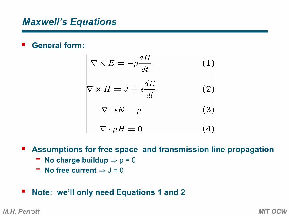
Maxwell’s Equations
General form:
Assumptions for free space and transmission line propagation- No charge buildup ⇒ ρ = 0- No free current ⇒ J = 0
Note: we’ll only need Equations 1 and 2
M.H. Perrott MIT OCW
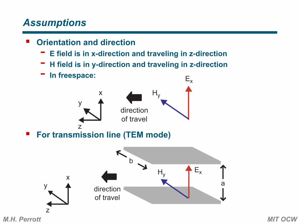
Assumptions
Orientation and direction- E field is in x-direction and traveling in z-direction- H field is in y-direction and traveling in z-direction- In freespace:
For transmission line (TEM mode)
yx
z
Ex
Hy
directionof travel
x
z
ExHy
b
ay directionof travel
M.H. Perrott MIT OCW
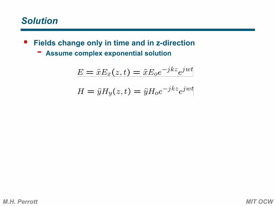
Solution
Fields change only in time and in z-direction- Assume complex exponential solution

M.H. Perrott MIT OCW
Solution
Fields change only in time and in z-direction- Assume complex exponential solution
Implications:
M.H. Perrott MIT OCW
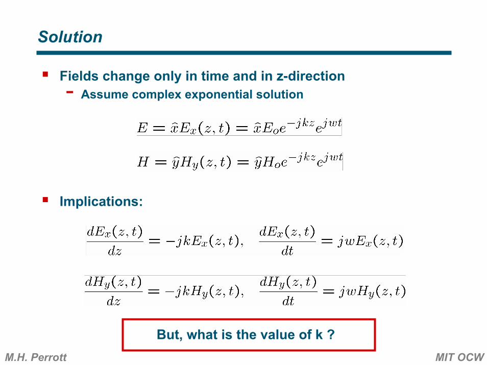
Solution
Fields change only in time and in z-direction- Assume complex exponential solution
Implications:
But, what is the value of k ?
M.H. Perrott MIT OCW
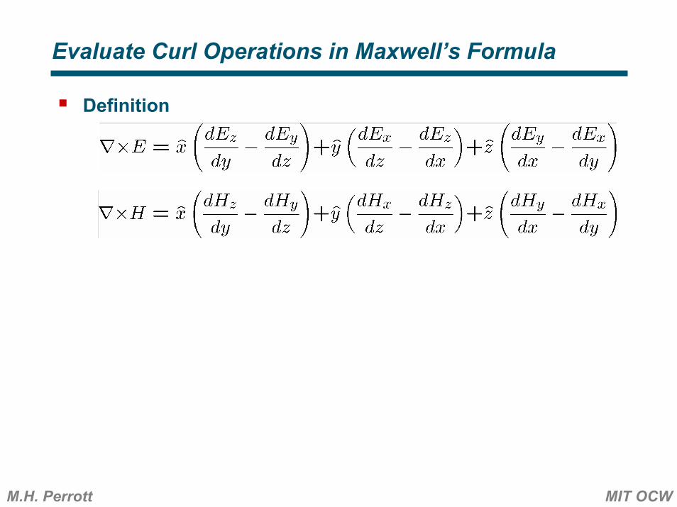
Evaluate Curl Operations in Maxwell’s Formula
Definition
M.H. Perrott MIT OCW
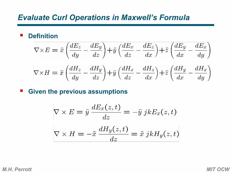
Evaluate Curl Operations in Maxwell’s Formula
Definition
Given the previous assumptions
M.H. Perrott MIT OCW
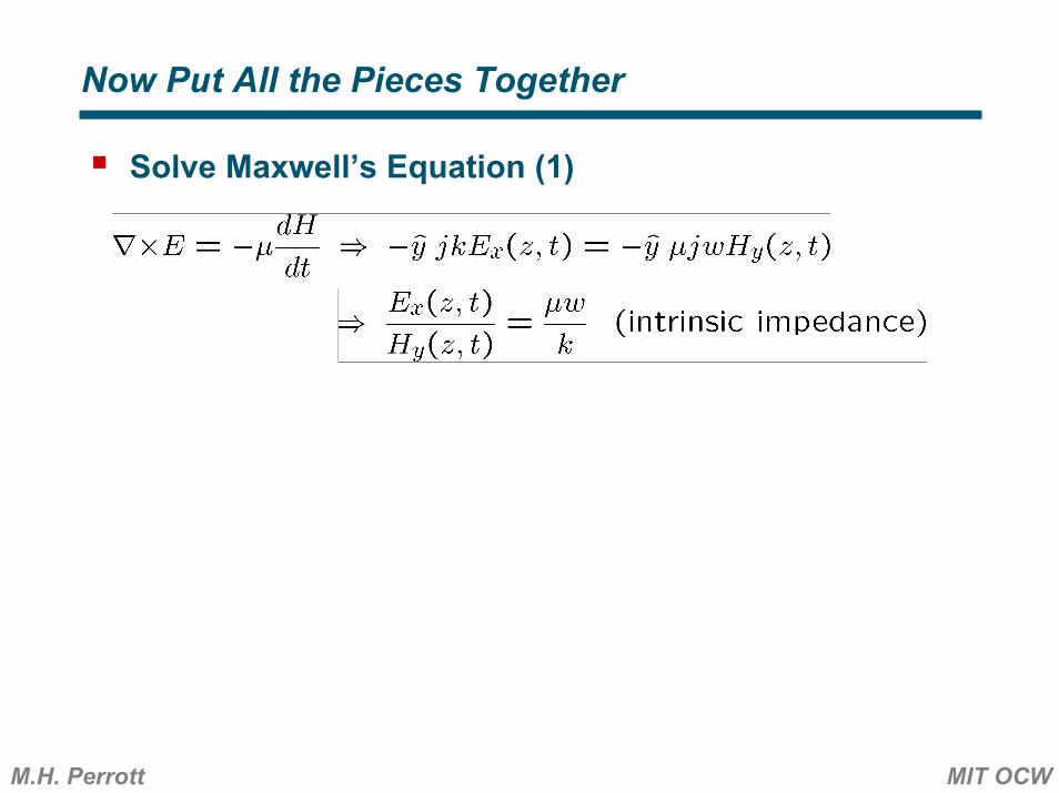
Now Put All the Pieces Together
Solve Maxwell’s Equation (1)
M.H. Perrott MIT OCW
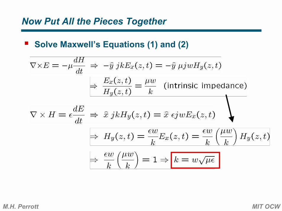
Now Put All the Pieces Together
Solve Maxwell’s Equations (1) and (2)
M.H. Perrott MIT OCW
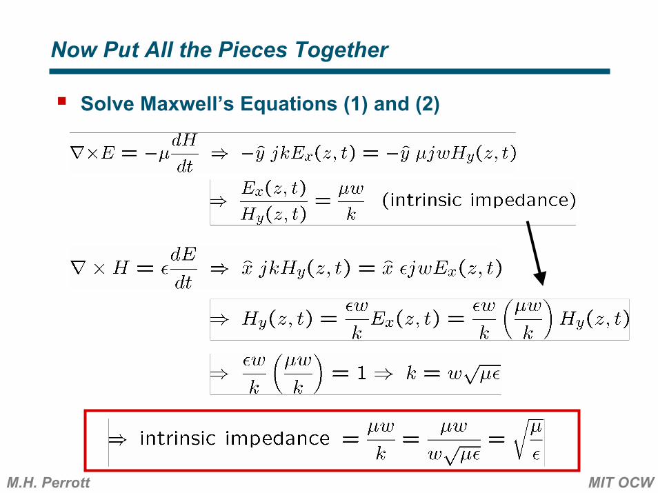
Now Put All the Pieces Together
Solve Maxwell’s Equations (1) and (2)
M.H. Perrott MIT OCW
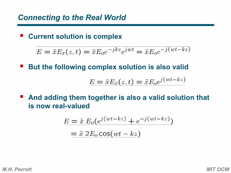
Connecting to the Real World
Current solution is complex
But the following complex solution is also valid
And adding them together is also a valid solution that is now real-valued
M.H. Perrott MIT OCW
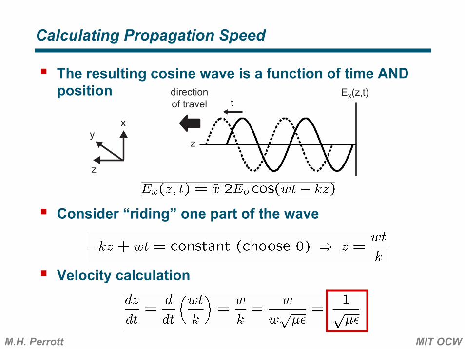
Calculating Propagation Speed
The resulting cosine wave is a function of time AND position
Consider “riding” one part of the wave
Velocity calculation
yx
z
directionof travel
z
tEx(z,t)
M.H. Perrott MIT OCW
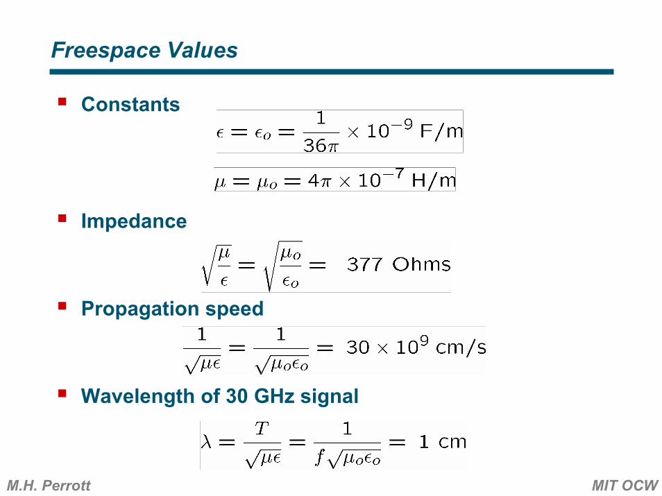
Freespace Values
Constants
Impedance
Propagation speed
Wavelength of 30 GHz signal
M.H. Perrott MIT OCW
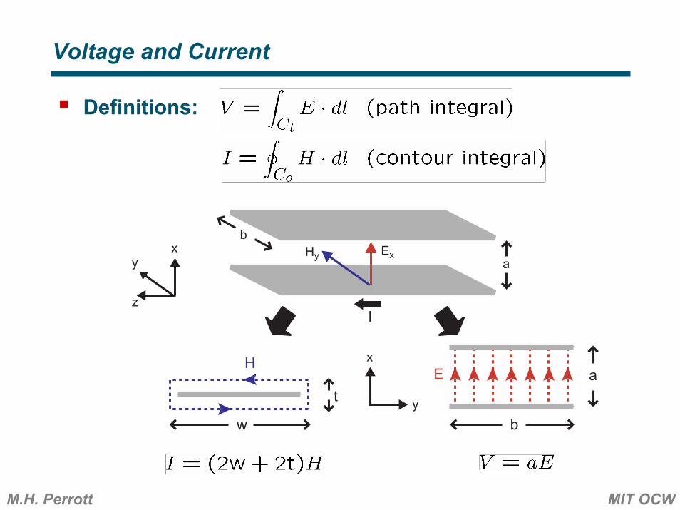
Voltage and Current
Definitions:
x
y
a
b
H
t
w
x
z
ExHy
b
ay
I
E
M.H. Perrott MIT OCW
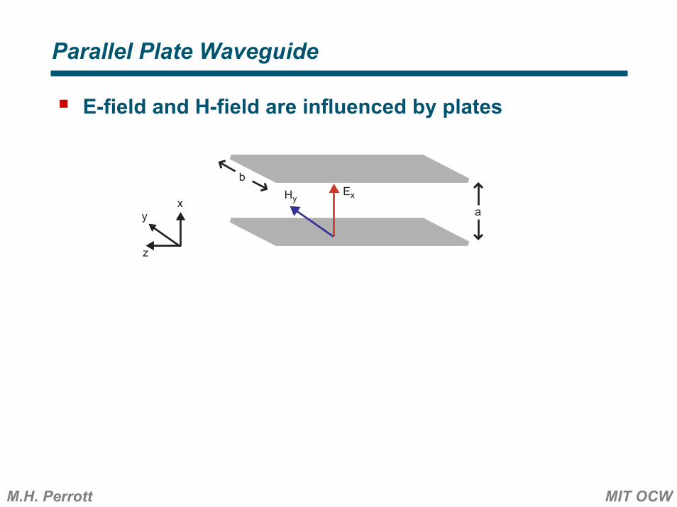
Parallel Plate Waveguide
E-field and H-field are influenced by plates
x
z
ExHy
b
ay
M.H. Perrott MIT OCW
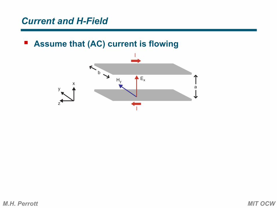
Current and H-Field
Assume that (AC) current is flowing
x
z
ExHy
b
ay
I
I
M.H. Perrott MIT OCW
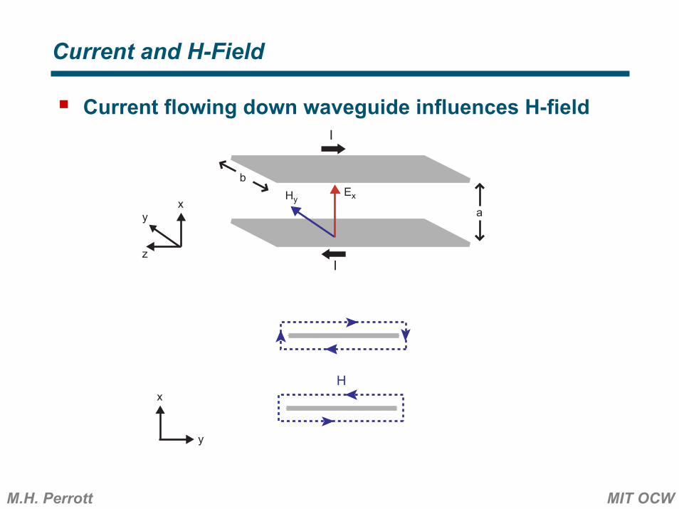
Current and H-Field
Current flowing down waveguide influences H-field
x
z
ExHy
b
ay
x
y
I
I
H
M.H. Perrott MIT OCW
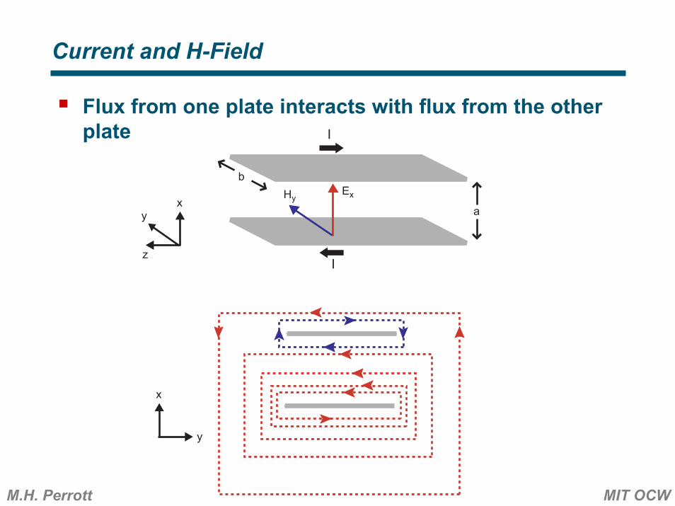
Current and H-Field
Flux from one plate interacts with flux from the other plate
x
z
ExHy
b
ay
x
y
I
I
M.H. Perrott MIT OCW
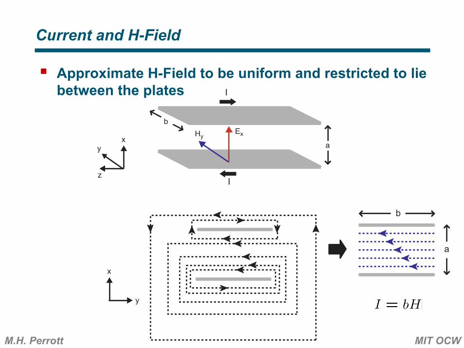
Current and H-Field
Approximate H-Field to be uniform and restricted to lie between the plates
x
z
ExHy
b
ay
x
y
a
b
I
I
M.H. Perrott MIT OCW
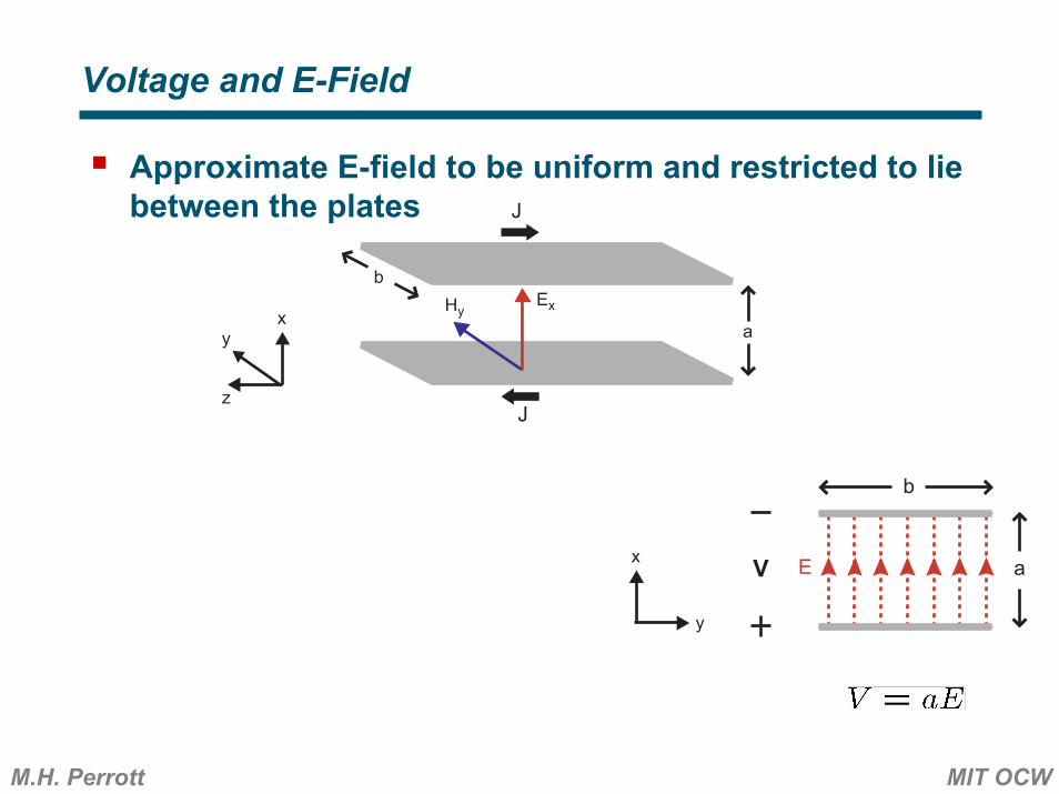
Voltage and E-Field
Approximate E-field to be uniform and restricted to lie between the plates
x
z
ExHy
b
ay
a
b
J
J
x
y
EV
M.H. Perrott MIT OCW
Back to Maxwell’s Equations
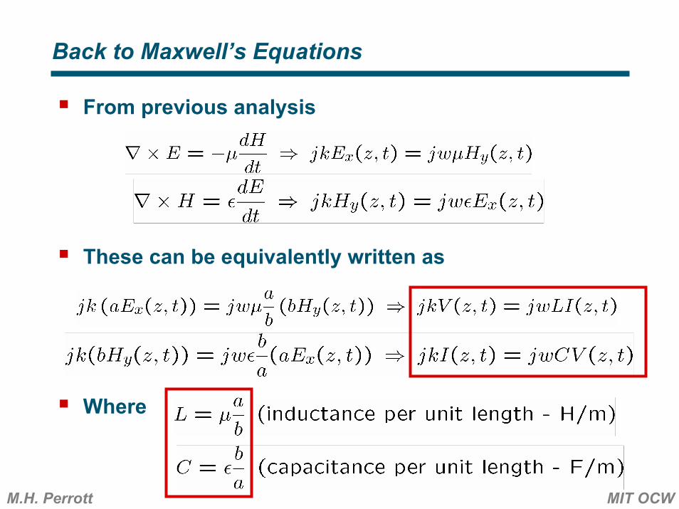
From previous analysis
These can be equivalently written as
Where
M.H. Perrott MIT OCW
Wave Equation for Transmission Line (TEM)
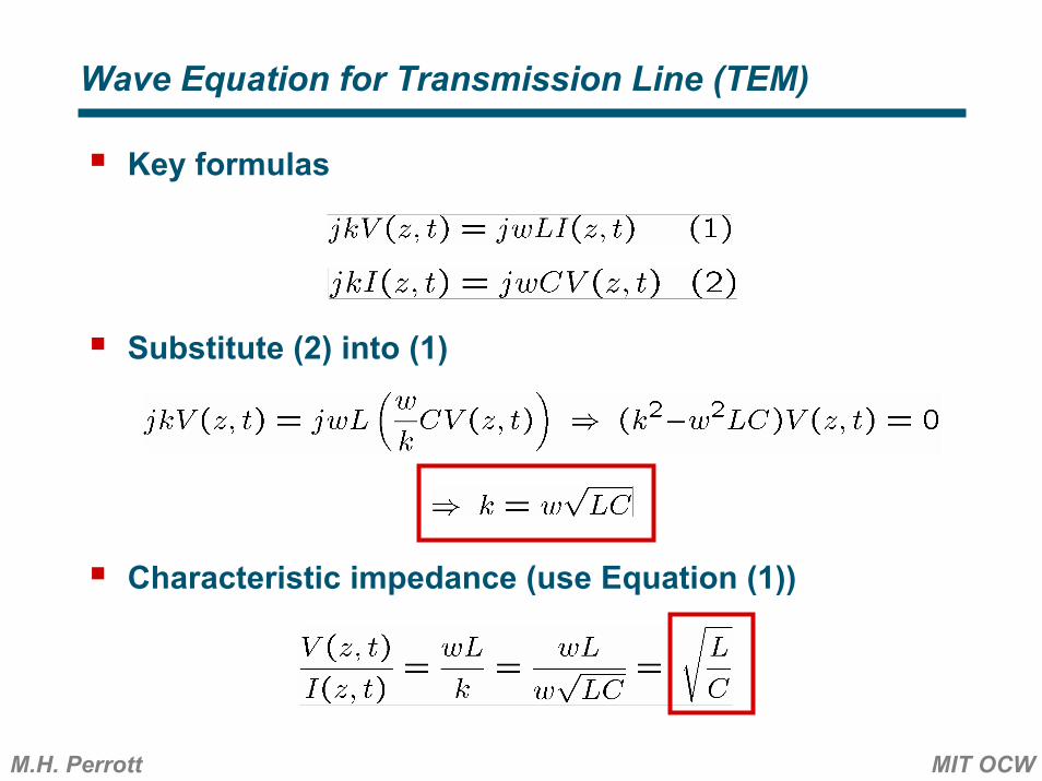
Key formulas
Substitute (2) into (1)
Characteristic impedance (use Equation (1))
M.H. Perrott MIT OCW
Connecting to the Real World
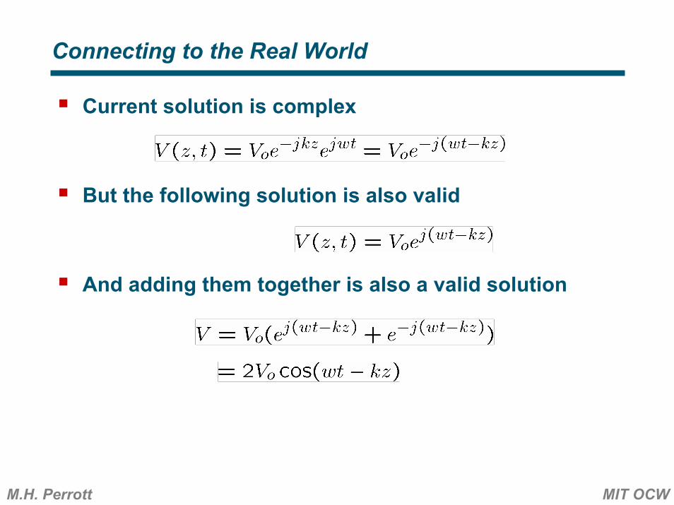
Current solution is complex
But the following solution is also valid
And adding them together is also a valid solution
M.H. Perrott MIT OCW
Calculating Propagation Speed
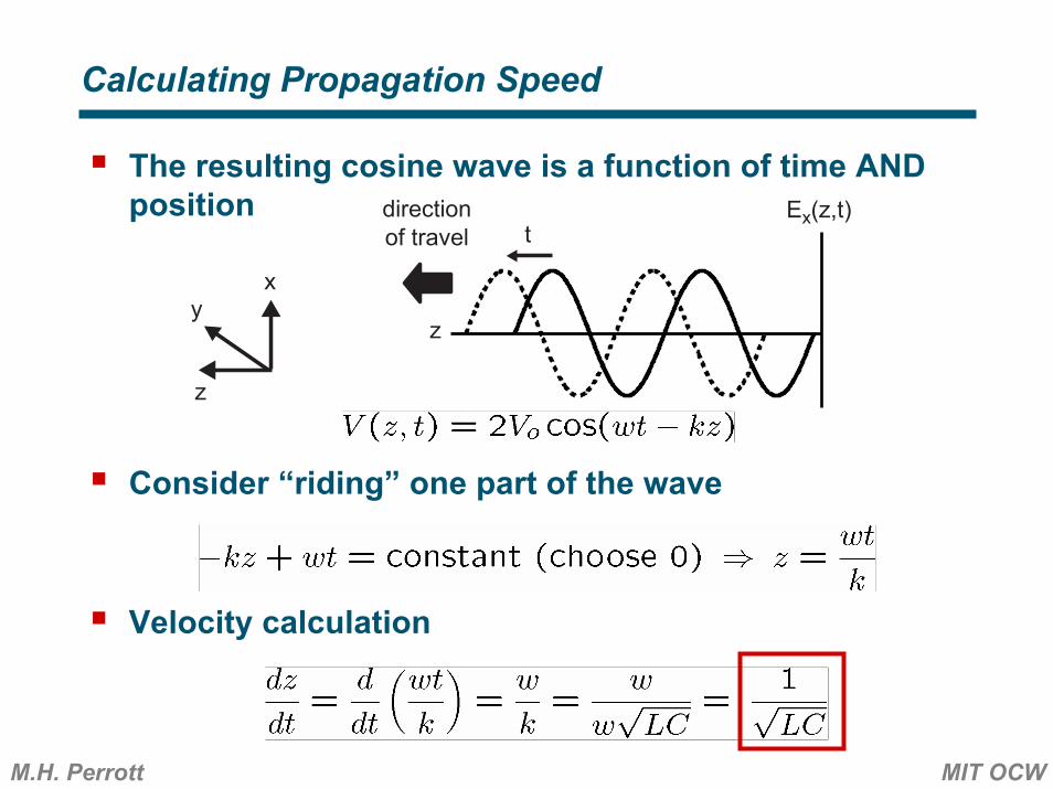
The resulting cosine wave is a function of time AND position
Consider “riding” one part of the wave
Velocity calculation
yx
z
directionof travel
z
tEx(z,t)
M.H. Perrott MIT OCW
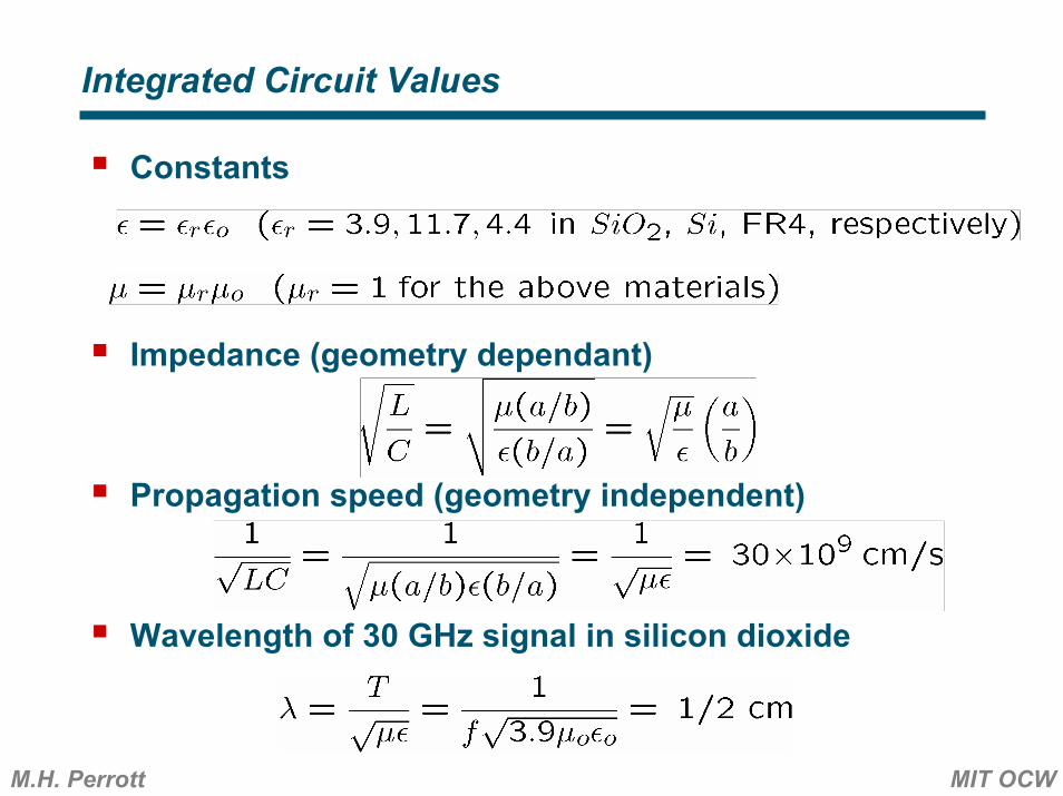
Integrated Circuit Values
Constants
Impedance (geometry dependant)
Propagation speed (geometry independent)
Wavelength of 30 GHz signal in silicon dioxide
M.H. Perrott MIT OCW
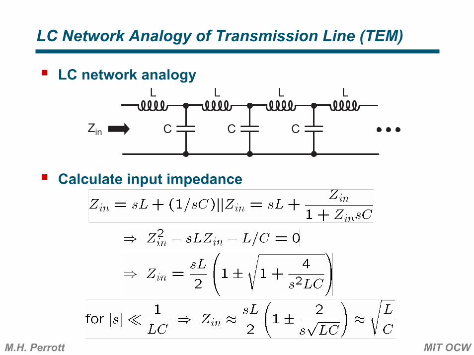
LC Network Analogy of Transmission Line (TEM)
LC network analogy
Calculate input impedance
L
C
L
C
L
C
L
Zin
M.H. Perrott MIT OCW
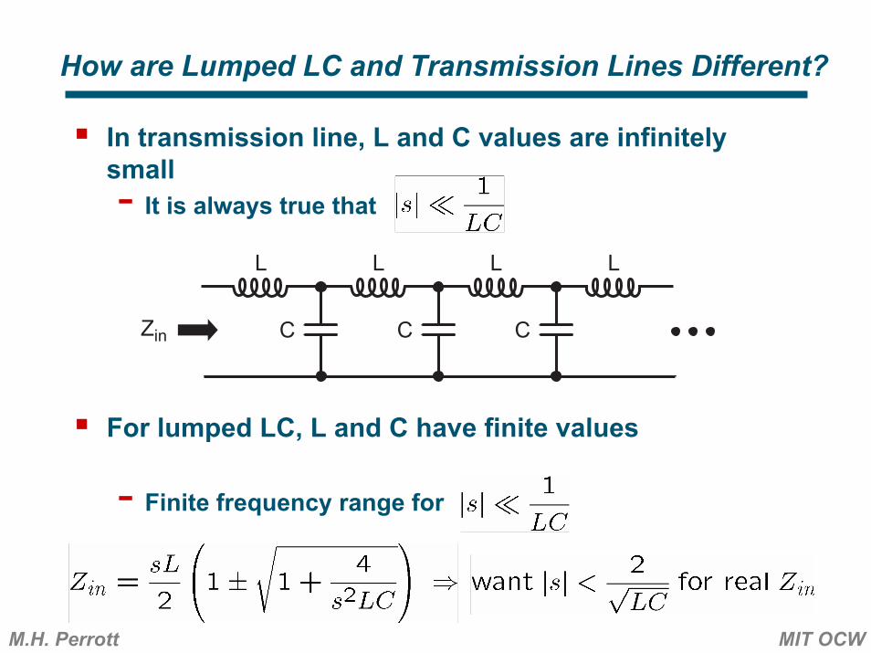
How are Lumped LC and Transmission Lines Different?
In transmission line, L and C values are infinitely small- It is always true that
For lumped LC, L and C have finite values
- Finite frequency range for
L
C
L
C
L
C
L
Zin
M.H. Perrott MIT OCW
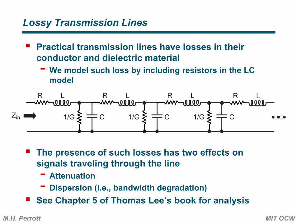
Lossy Transmission Lines
Practical transmission lines have losses in their conductor and dielectric material- We model such loss by including resistors in the LC
model
The presence of such losses has two effects on signals traveling through the line- Attenuation- Dispersion (i.e., bandwidth degradation)
See Chapter 5 of Thomas Lee’s book for analysis
Zin 1/G
L
C
R
1/G
L
C
R
1/G
L
C
R LR