6. ANalysis Of VAriance (ANOVA) · 2019-10-29 · What do these ANOVA F statistics test? 1st...
59
6. AN alysis O f VA riance (ANOVA) Copyright c 2019 Dan Nettleton (Iowa State University) 6. Statistics 510 1 / 59
Transcript of 6. ANalysis Of VAriance (ANOVA) · 2019-10-29 · What do these ANOVA F statistics test? 1st...

6. ANalysis Of VAriance(ANOVA)
Copyright c©2019 Dan Nettleton (Iowa State University) 6. Statistics 510 1 / 59
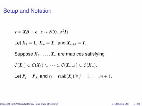
Setup and Notation
y = Xβ + ε, ε ∼ N(0, σ2I)
Let X1 = 1, Xm = X, and Xm+1 = I.
Suppose X2, . . . ,Xm are matrices satisfying
C(X1) ⊂ C(X2) ⊂ · · · ⊂ C(Xm−1) ⊂ C(Xm).
Let Pj = PXj and rj = rank(Xj) ∀ j = 1, . . . ,m + 1.
Copyright c©2019 Dan Nettleton (Iowa State University) 6. Statistics 510 2 / 59
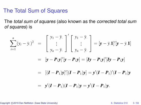
The Total Sum of Squares
The total sum of squares (also known as the corrected total sumof squares) is
n∑i=1
(yi − y·)2 =
y1 − y·...
yn − y·
′ y1 − y·...
yn − y·
= [y− y·1]′[y− y·1]
= [y− P1y]′[y− P1y] = [Iy− P1y]′[Iy− P1y]
= [(I − P1)y]′[(I − P1)y] = y′(I − P1)′(I − P1)y
= y′(I − P1)(I − P1)y = y′(I − P1)y.
Copyright c©2019 Dan Nettleton (Iowa State University) 6. Statistics 510 3 / 59
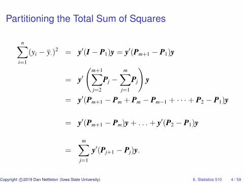
Partitioning the Total Sum of Squares
n∑i=1
(yi − y·)2 = y′(I − P1)y = y′(Pm+1 − P1)y
= y′(
m+1∑j=2
Pj −m∑
j=1
Pj
)y
= y′(Pm+1 − Pm + Pm − Pm−1 + · · ·+ P2 − P1)y
= y′(Pm+1 − Pm)y + . . .+ y′(P2 − P1)y
=m∑
j=1
y′(Pj+1 − Pj)y.
Copyright c©2019 Dan Nettleton (Iowa State University) 6. Statistics 510 4 / 59
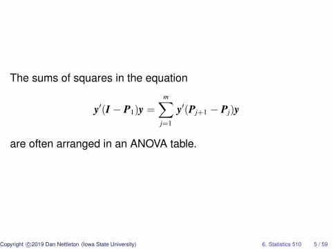
The sums of squares in the equation
y′(I − P1)y =m∑
j=1
y′(Pj+1 − Pj)y
are often arranged in an ANOVA table.
Copyright c©2019 Dan Nettleton (Iowa State University) 6. Statistics 510 5 / 59
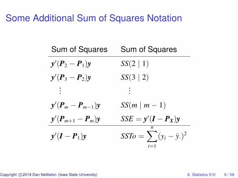
Some Additional Sum of Squares Notation
Sum of Squares Sum of Squares
y′(P2 − P1)y SS(2 | 1)
y′(P3 − P2)y SS(3 | 2)...
...
y′(Pm − Pm−1)y SS(m | m− 1)
y′(Pm+1 − Pm)y SSE = y′(I − PX)y
y′(I − P1)y SSTo =n∑
i=1
(yi − y·)2
Copyright c©2019 Dan Nettleton (Iowa State University) 6. Statistics 510 6 / 59
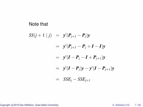
Note that
SS(j + 1 | j) = y′(Pj+1 − Pj)y
= y′(Pj+1 − Pj + I − I)y
= y′(I − Pj − I + Pj+1)y
= y′(I − Pj)y− y′(I − Pj+1)y
= SSEj − SSEj+1
Copyright c©2019 Dan Nettleton (Iowa State University) 6. Statistics 510 7 / 59
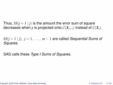
Thus, SS(j + 1 | j) is the amount the error sum of squaredecreases when y is projected onto C(Xj+1) instead of C(Xj).
SS(j + 1 | j), j = 1, . . . , m− 1 are called Sequential Sums ofSquares.
SAS calls these Type I Sums of Squares.
Copyright c©2019 Dan Nettleton (Iowa State University) 6. Statistics 510 8 / 59
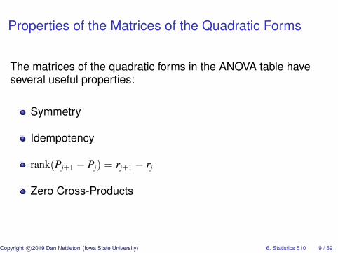
Properties of the Matrices of the Quadratic Forms
The matrices of the quadratic forms in the ANOVA table haveseveral useful properties:
Symmetry
Idempotency
rank(Pj+1 − Pj) = rj+1 − rj
Zero Cross-Products
Copyright c©2019 Dan Nettleton (Iowa State University) 6. Statistics 510 9 / 59
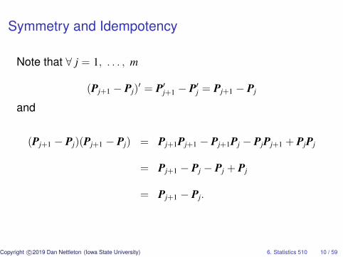
Symmetry and Idempotency
Note that ∀ j = 1, . . . , m
(Pj+1 − Pj)′ = P′j+1 − P′j = Pj+1 − Pj
and
(Pj+1 − Pj)(Pj+1 − Pj) = Pj+1Pj+1 − Pj+1Pj − PjPj+1 + PjPj
= Pj+1 − Pj − Pj + Pj
= Pj+1 − Pj.
Copyright c©2019 Dan Nettleton (Iowa State University) 6. Statistics 510 10 / 59
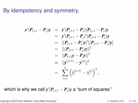
By idempotency and symmetry,
y′(Pj+1 − Pj)y = y′(Pj+1 − Pj)(Pj+1 − Pj)y= y′(Pj+1 − Pj)
′(Pj+1 − Pj)y= [(Pj+1 − Pj)y]′[(Pj+1 − Pj)y]
= ||(Pj+1 − Pj)y||2
= ||Pj+1y− Pjy||2
≡ ||y(j+1) − y(j)||2
=n∑
i=1
(y(j+1)
i − y(j)i
)2,
which is why we call y′(Pj+1 − Pj)y a “sum of squares.”
Copyright c©2019 Dan Nettleton (Iowa State University) 6. Statistics 510 11 / 59
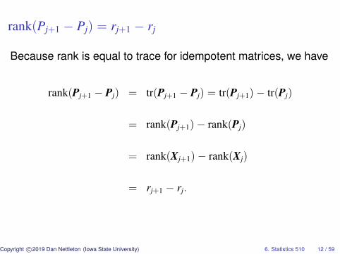
rank(Pj+1 − Pj) = rj+1 − rj
Because rank is equal to trace for idempotent matrices, we have
rank(Pj+1 − Pj) = tr(Pj+1 − Pj) = tr(Pj+1)− tr(Pj)
= rank(Pj+1)− rank(Pj)
= rank(Xj+1)− rank(Xj)
= rj+1 − rj.
Copyright c©2019 Dan Nettleton (Iowa State University) 6. Statistics 510 12 / 59
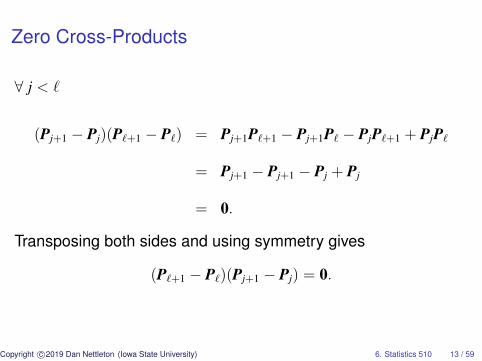
Zero Cross-Products
∀ j < `
(Pj+1 − Pj)(P`+1 − P`) = Pj+1P`+1 − Pj+1P` − PjP`+1 + PjP`
= Pj+1 − Pj+1 − Pj + Pj
= 0.
Transposing both sides and using symmetry gives
(P`+1 − P`)(Pj+1 − Pj) = 0.
Copyright c©2019 Dan Nettleton (Iowa State University) 6. Statistics 510 13 / 59
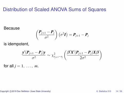
Distribution of Scaled ANOVA Sums of Squares
Because (Pj+1 − Pj
σ2
)(σ2I)
= Pj+1 − Pj
is idempotent,
y′(Pj+1 − Pj)yσ2 ∼ χ2
rj+1−rj
(β′X′(Pj+1 − Pj)Xβ
2σ2
)for all j = 1, . . . , m.
Copyright c©2019 Dan Nettleton (Iowa State University) 6. Statistics 510 14 / 59
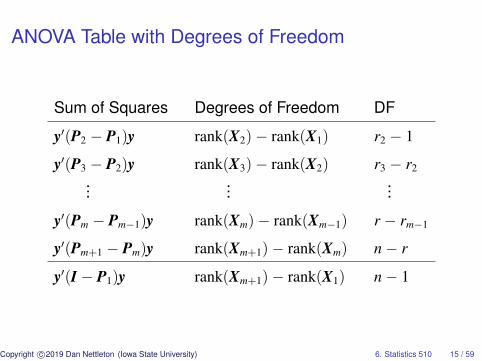
ANOVA Table with Degrees of Freedom
Sum of Squares Degrees of Freedom DF
y′(P2 − P1)y rank(X2)− rank(X1) r2 − 1
y′(P3 − P2)y rank(X3)− rank(X2) r3 − r2...
......
y′(Pm − Pm−1)y rank(Xm)− rank(Xm−1) r − rm−1
y′(Pm+1 − Pm)y rank(Xm+1)− rank(Xm) n− r
y′(I − P1)y rank(Xm+1)− rank(X1) n− 1
Copyright c©2019 Dan Nettleton (Iowa State University) 6. Statistics 510 15 / 59
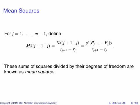
Mean Squares
For j = 1, . . . , m− 1, define
MS(j + 1 | j) =SS(j + 1 | j)
rj+1 − rj=
y′(Pj+1 − Pj)yrj+1 − rj
.
These sums of squares divided by their degrees of freedom areknown as mean squares.
Copyright c©2019 Dan Nettleton (Iowa State University) 6. Statistics 510 16 / 59
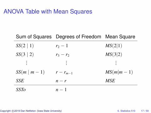
ANOVA Table with Mean Squares
Sum of Squares Degrees of Freedom Mean Square
SS(2 | 1) r2 − 1 MS(2|1)
SS(3 | 2) r3 − r2 MS(3|2)...
......
SS(m | m− 1) r − rm−1 MS(m|m− 1)
SSE n− r MSE
SSTo n− 1
Copyright c©2019 Dan Nettleton (Iowa State University) 6. Statistics 510 17 / 59
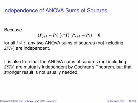
Independence of ANOVA Sums of Squares
Because(Pj+1 − Pj)
(σ2I)
(P`+1 − P`) = 0
for all j 6= `, any two ANOVA sums of squares (not includingSSTo) are independent.
It is also true that the ANOVA sums of squares (not includingSSTo) are mutually independent by Cochran’s Theorem, but thatstronger result is not usually needed.
Copyright c©2019 Dan Nettleton (Iowa State University) 6. Statistics 510 18 / 59
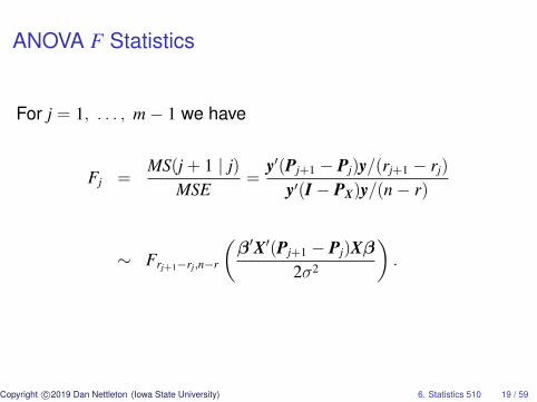
ANOVA F Statistics
For j = 1, . . . , m− 1 we have
Fj =MS(j + 1 | j)
MSE=
y′(Pj+1 − Pj)y/(rj+1 − rj)
y′(I − PX)y/(n− r)
∼ Frj+1−rj,n−r
(β′X′(Pj+1 − Pj)Xβ
2σ2
).
Copyright c©2019 Dan Nettleton (Iowa State University) 6. Statistics 510 19 / 59
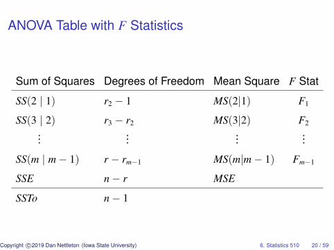
ANOVA Table with F Statistics
Sum of Squares Degrees of Freedom Mean Square F Stat
SS(2 | 1) r2 − 1 MS(2|1) F1
SS(3 | 2) r3 − r2 MS(3|2) F2...
......
...
SS(m | m− 1) r − rm−1 MS(m|m− 1) Fm−1
SSE n− r MSE
SSTo n− 1
Copyright c©2019 Dan Nettleton (Iowa State University) 6. Statistics 510 20 / 59
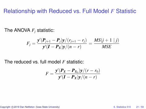
Relationship with Reduced vs. Full Model F Statistic
The ANOVA Fj statistic:
Fj =y′(Pj+1 − Pj)y/(rj+1 − rj)
y′(I − PX)y/(n− r)=
MS(j + 1 | j)MSE
The reduced vs. full model F statistic:
F =y′(PX − PX0)y/(r − r0)
y′(I − PX)y/(n− r)
Copyright c©2019 Dan Nettleton (Iowa State University) 6. Statistics 510 21 / 59
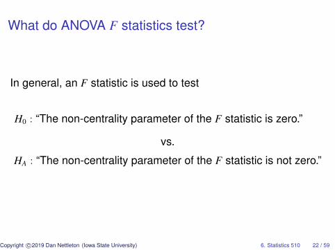
What do ANOVA F statistics test?
In general, an F statistic is used to test
H0 : “The non-centrality parameter of the F statistic is zero.”
vs.
HA : “The non-centrality parameter of the F statistic is not zero.”
Copyright c©2019 Dan Nettleton (Iowa State University) 6. Statistics 510 22 / 59
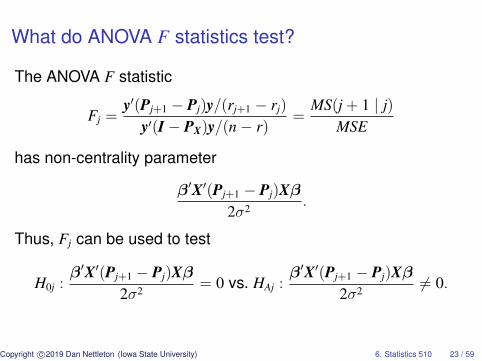
What do ANOVA F statistics test?
The ANOVA F statistic
Fj =y′(Pj+1 − Pj)y/(rj+1 − rj)
y′(I − PX)y/(n− r)=
MS(j + 1 | j)MSE
has non-centrality parameter
β′X′(Pj+1 − Pj)Xβ
2σ2 .
Thus, Fj can be used to test
H0j :β′X′(Pj+1 − Pj)Xβ
2σ2 = 0 vs. HAj :β′X′(Pj+1 − Pj)Xβ
2σ2 6= 0.
Copyright c©2019 Dan Nettleton (Iowa State University) 6. Statistics 510 23 / 59
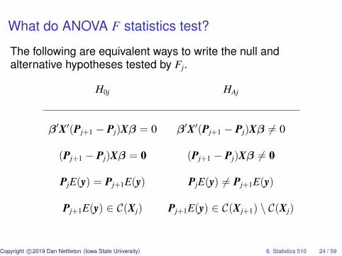
What do ANOVA F statistics test?
The following are equivalent ways to write the null andalternative hypotheses tested by Fj.
H0j HAj
β′X′(Pj+1 − Pj)Xβ = 0 β′X′(Pj+1 − Pj)Xβ 6= 0
(Pj+1 − Pj)Xβ = 0 (Pj+1 − Pj)Xβ 6= 0
PjE(y) = Pj+1E(y) PjE(y) 6= Pj+1E(y)
Pj+1E(y) ∈ C(Xj) Pj+1E(y) ∈ C(Xj+1) \ C(Xj)
Copyright c©2019 Dan Nettleton (Iowa State University) 6. Statistics 510 24 / 59
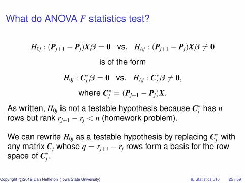
What do ANOVA F statistics test?
H0j : (Pj+1 − Pj)Xβ = 0 vs. HAj : (Pj+1 − Pj)Xβ 6= 0
is of the form
H0j : C∗j β = 0 vs. HAj : C∗j β 6= 0,
where C∗j = (Pj+1 − Pj)X.
As written, H0j is not a testable hypothesis because C∗j has nrows but rank rj+1 − rj < n (homework problem).
We can rewrite H0j as a testable hypothesis by replacing C∗j withany matrix Cj whose q = rj+1 − rj rows form a basis for the rowspace of C∗j .
Copyright c©2019 Dan Nettleton (Iowa State University) 6. Statistics 510 25 / 59
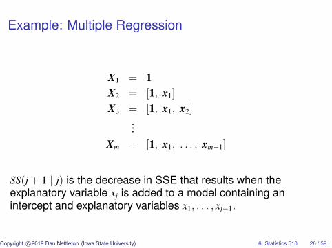
Example: Multiple Regression
X1 = 1X2 = [1, x1]
X3 = [1, x1, x2]...
Xm = [1, x1, . . . , xm−1]
SS(j + 1 | j) is the decrease in SSE that results when theexplanatory variable xj is added to a model containing anintercept and explanatory variables x1, . . . , xj−1.
Copyright c©2019 Dan Nettleton (Iowa State University) 6. Statistics 510 26 / 59
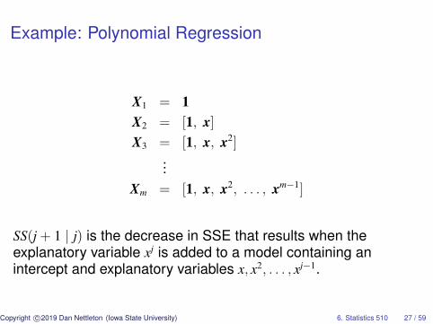
Example: Polynomial Regression
X1 = 1X2 = [1, x]
X3 = [1, x, x2]...
Xm = [1, x, x2, . . . , xm−1]
SS(j + 1 | j) is the decrease in SSE that results when theexplanatory variable xj is added to a model containing anintercept and explanatory variables x, x2, . . . , xj−1.
Copyright c©2019 Dan Nettleton (Iowa State University) 6. Statistics 510 27 / 59
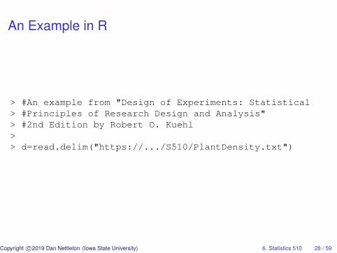
An Example in R
> #An example from "Design of Experiments: Statistical> #Principles of Research Design and Analysis"> #2nd Edition by Robert O. Kuehl>> d=read.delim("https://.../S510/PlantDensity.txt")
Copyright c©2019 Dan Nettleton (Iowa State University) 6. Statistics 510 28 / 59
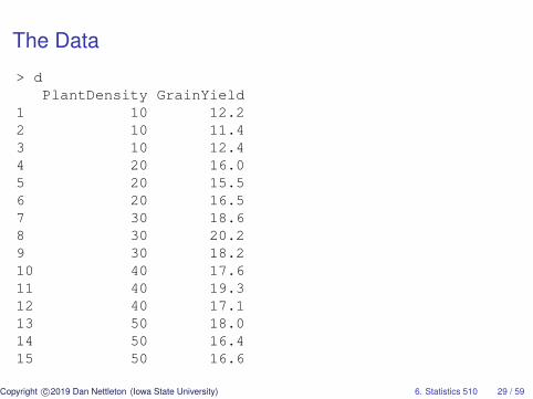
The Data
> dPlantDensity GrainYield
1 10 12.22 10 11.43 10 12.44 20 16.05 20 15.56 20 16.57 30 18.68 30 20.29 30 18.210 40 17.611 40 19.312 40 17.113 50 18.014 50 16.415 50 16.6
Copyright c©2019 Dan Nettleton (Iowa State University) 6. Statistics 510 29 / 59
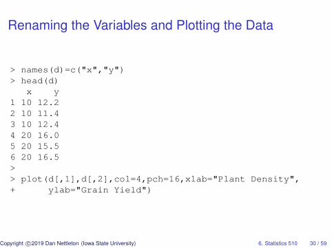
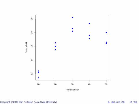
Renaming the Variables and Plotting the Data
> names(d)=c("x","y")> head(d)
x y1 10 12.22 10 11.43 10 12.44 20 16.05 20 15.56 20 16.5>> plot(d[,1],d[,2],col=4,pch=16,xlab="Plant Density",+ ylab="Grain Yield")
Copyright c©2019 Dan Nettleton (Iowa State University) 6. Statistics 510 30 / 59
●
●
●
●
●
●
●
●
●
●
●
●
●
●●
10 20 30 40 50
1214
1618
20
Plant Density
Gra
in Y
ield
Copyright c©2019 Dan Nettleton (Iowa State University) 6. Statistics 510 31 / 59
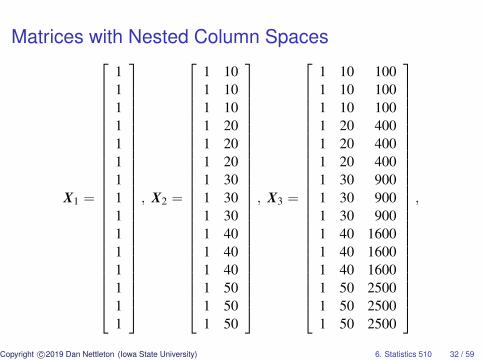
Matrices with Nested Column Spaces
X1 =
111111111111111
, X2 =
1 101 101 101 201 201 201 301 301 301 401 401 401 501 501 50
, X3 =
1 10 1001 10 1001 10 1001 20 4001 20 4001 20 4001 30 9001 30 9001 30 9001 40 16001 40 16001 40 16001 50 25001 50 25001 50 2500
,
Copyright c©2019 Dan Nettleton (Iowa State University) 6. Statistics 510 32 / 59
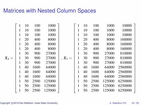
Matrices with Nested Column Spaces
X4 =
1 10 100 10001 10 100 10001 10 100 10001 20 400 80001 20 400 80001 20 400 80001 30 900 270001 30 900 270001 30 900 270001 40 1600 640001 40 1600 640001 40 1600 640001 50 2500 1250001 50 2500 1250001 50 2500 125000
, X5 =
1 10 100 1000 100001 10 100 1000 100001 10 100 1000 100001 20 400 8000 1600001 20 400 8000 1600001 20 400 8000 1600001 30 900 27000 8100001 30 900 27000 8100001 30 900 27000 8100001 40 1600 64000 25600001 40 1600 64000 25600001 40 1600 64000 25600001 50 2500 125000 62500001 50 2500 125000 62500001 50 2500 125000 6250000
Copyright c©2019 Dan Nettleton (Iowa State University) 6. Statistics 510 33 / 59
Centering and Standardizing for Numerical Stability
It is typically best for numerical stability to center and scale aquantitative explanatory variable prior to computing higher orderterms.
In the plant density example, we could replace x by (x− 30)/10and work with the matrices on the next two slides.
Because these matrices have the same column spaces as theoriginal matrices, the ANOVA table entries are mathematicallyidentical for either set of matrices.
Copyright c©2019 Dan Nettleton (Iowa State University) 6. Statistics 510 34 / 59
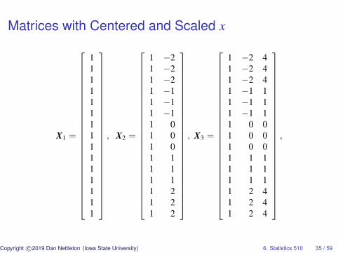
Matrices with Centered and Scaled x
X1 =
111111111111111
, X2 =
1 −21 −21 −21 −11 −11 −11 01 01 01 11 11 11 21 21 2
, X3 =
1 −2 41 −2 41 −2 41 −1 11 −1 11 −1 11 0 01 0 01 0 01 1 11 1 11 1 11 2 41 2 41 2 4
,
Copyright c©2019 Dan Nettleton (Iowa State University) 6. Statistics 510 35 / 59
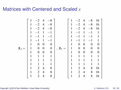
Matrices with Centered and Scaled x
X4 =
1 −2 4 −81 −2 4 −81 −2 4 −81 −1 1 −11 −1 1 −11 −1 1 −11 0 0 01 0 0 01 0 0 01 1 1 11 1 1 11 1 1 11 2 4 81 2 4 81 2 4 8
, X5 =
1 −2 4 −8 161 −2 4 −8 161 −2 4 −8 161 −1 1 −1 11 −1 1 −1 11 −1 1 −1 11 0 0 0 01 0 0 0 01 0 0 0 01 1 1 1 11 1 1 1 11 1 1 1 11 2 4 8 161 2 4 8 161 2 4 8 16
Copyright c©2019 Dan Nettleton (Iowa State University) 6. Statistics 510 36 / 59
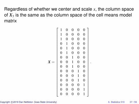
Regardless of whether we center and scale x, the column spaceof X5 is the same as the column space of the cell means modelmatrix
X =
1 0 0 0 01 0 0 0 01 0 0 0 00 1 0 0 00 1 0 0 00 1 0 0 00 0 1 0 00 0 1 0 00 0 1 0 00 0 0 1 00 0 0 1 00 0 0 1 00 0 0 0 10 0 0 0 10 0 0 0 1
.
Copyright c©2019 Dan Nettleton (Iowa State University) 6. Statistics 510 37 / 59
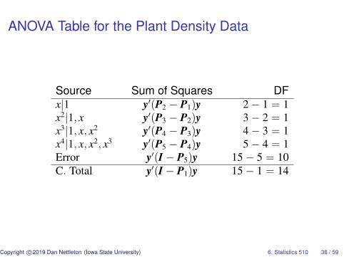
ANOVA Table for the Plant Density Data
Source Sum of Squares DFx|1 y′(P2 − P1)y 2− 1 = 1x2|1, x y′(P3 − P2)y 3− 2 = 1x3|1, x, x2 y′(P4 − P3)y 4− 3 = 1x4|1, x, x2, x3 y′(P5 − P4)y 5− 4 = 1Error y′(I − P5)y 15− 5 = 10C. Total y′(I − P1)y 15− 1 = 14
Copyright c©2019 Dan Nettleton (Iowa State University) 6. Statistics 510 38 / 59
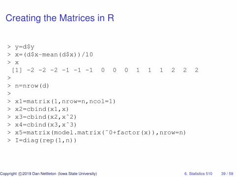
Creating the Matrices in R
> y=d$y> x=(d$x-mean(d$x))/10> x[1] -2 -2 -2 -1 -1 -1 0 0 0 1 1 1 2 2 2
>> n=nrow(d)>> x1=matrix(1,nrow=n,ncol=1)> x2=cbind(x1,x)> x3=cbind(x2,xˆ2)> x4=cbind(x3,xˆ3)> x5=matrix(model.matrix(˜0+factor(x)),nrow=n)> I=diag(rep(1,n))
Copyright c©2019 Dan Nettleton (Iowa State University) 6. Statistics 510 39 / 59
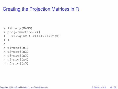
Creating the Projection Matrices in R
> library(MASS)> proj=function(x){+ x%*%ginv(t(x)%*%x)%*%t(x)+ }>> p1=proj(x1)> p2=proj(x2)> p3=proj(x3)> p4=proj(x4)> p5=proj(x5)
Copyright c©2019 Dan Nettleton (Iowa State University) 6. Statistics 510 40 / 59
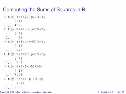
Computing the Sums of Squares in R> t(y)%*%(p2-p1)%*%y
[,1][1,] 43.2> t(y)%*%(p3-p2)%*%y
[,1][1,] 42> t(y)%*%(p4-p3)%*%y
[,1][1,] 0.3> t(y)%*%(p5-p4)%*%y
[,1][1,] 2.1> t(y)%*%(I-p5)%*%y
[,1][1,] 7.48> t(y)%*%(I-p1)%*%y
[,1][1,] 95.08
Copyright c©2019 Dan Nettleton (Iowa State University) 6. Statistics 510 41 / 59
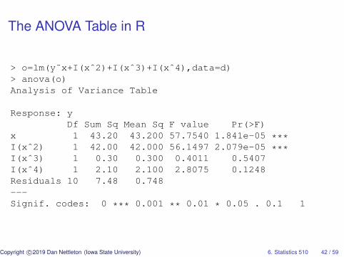
The ANOVA Table in R
> o=lm(y˜x+I(xˆ2)+I(xˆ3)+I(xˆ4),data=d)> anova(o)Analysis of Variance Table
Response: yDf Sum Sq Mean Sq F value Pr(>F)
x 1 43.20 43.200 57.7540 1.841e-05 ***I(xˆ2) 1 42.00 42.000 56.1497 2.079e-05 ***I(xˆ3) 1 0.30 0.300 0.4011 0.5407I(xˆ4) 1 2.10 2.100 2.8075 0.1248Residuals 10 7.48 0.748---Signif. codes: 0 *** 0.001 ** 0.01 * 0.05 . 0.1 1
Copyright c©2019 Dan Nettleton (Iowa State University) 6. Statistics 510 42 / 59
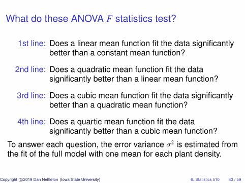
What do these ANOVA F statistics test?
1st line: Does a linear mean function fit the data significantlybetter than a constant mean function?
2nd line: Does a quadratic mean function fit the datasignificantly better than a linear mean function?
3rd line: Does a cubic mean function fit the data significantlybetter than a quadratic mean function?
4th line: Does a quartic mean function fit the datasignificantly better than a cubic mean function?
To answer each question, the error variance σ2 is estimated fromthe fit of the full model with one mean for each plant density.
Copyright c©2019 Dan Nettleton (Iowa State University) 6. Statistics 510 43 / 59
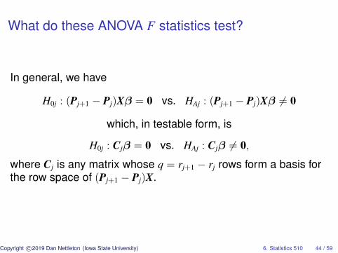
What do these ANOVA F statistics test?
In general, we have
H0j : (Pj+1 − Pj)Xβ = 0 vs. HAj : (Pj+1 − Pj)Xβ 6= 0
which, in testable form, is
H0j : Cjβ = 0 vs. HAj : Cjβ 6= 0,
where Cj is any matrix whose q = rj+1 − rj rows form a basis forthe row space of (Pj+1 − Pj)X.
Copyright c©2019 Dan Nettleton (Iowa State University) 6. Statistics 510 44 / 59
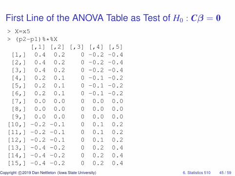
First Line of the ANOVA Table as Test of H0 : Cβ = 0> X=x5> (p2-p1)%*%X
[,1] [,2] [,3] [,4] [,5][1,] 0.4 0.2 0 -0.2 -0.4[2,] 0.4 0.2 0 -0.2 -0.4[3,] 0.4 0.2 0 -0.2 -0.4[4,] 0.2 0.1 0 -0.1 -0.2[5,] 0.2 0.1 0 -0.1 -0.2[6,] 0.2 0.1 0 -0.1 -0.2[7,] 0.0 0.0 0 0.0 0.0[8,] 0.0 0.0 0 0.0 0.0[9,] 0.0 0.0 0 0.0 0.0
[10,] -0.2 -0.1 0 0.1 0.2[11,] -0.2 -0.1 0 0.1 0.2[12,] -0.2 -0.1 0 0.1 0.2[13,] -0.4 -0.2 0 0.2 0.4[14,] -0.4 -0.2 0 0.2 0.4[15,] -0.4 -0.2 0 0.2 0.4
Copyright c©2019 Dan Nettleton (Iowa State University) 6. Statistics 510 45 / 59
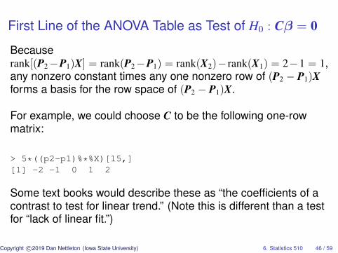
First Line of the ANOVA Table as Test of H0 : Cβ = 0
Becauserank[(P2−P1)X] = rank(P2−P1) = rank(X2)− rank(X1) = 2−1 = 1,any nonzero constant times any one nonzero row of (P2 − P1)Xforms a basis for the row space of (P2 − P1)X.
For example, we could choose C to be the following one-rowmatrix:
> 5*((p2-p1)%*%X)[15,][1] -2 -1 0 1 2
Some text books would describe these as “the coefficients of acontrast to test for linear trend.” (Note this is different than a testfor “lack of linear fit.”)
Copyright c©2019 Dan Nettleton (Iowa State University) 6. Statistics 510 46 / 59
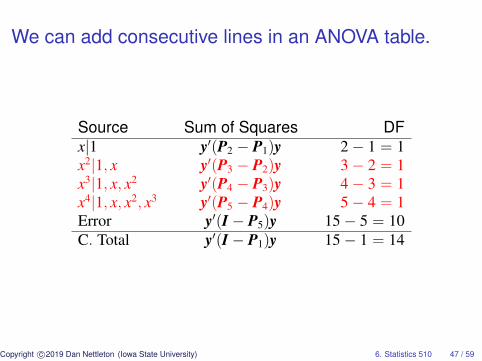
We can add consecutive lines in an ANOVA table.
Source Sum of Squares DFx|1 y′(P2 − P1)y 2− 1 = 1x2|1, x y′(P3 − P2)y 3− 2 = 1x3|1, x, x2 y′(P4 − P3)y 4− 3 = 1x4|1, x, x2, x3 y′(P5 − P4)y 5− 4 = 1Error y′(I − P5)y 15− 5 = 10C. Total y′(I − P1)y 15− 1 = 14
Copyright c©2019 Dan Nettleton (Iowa State University) 6. Statistics 510 47 / 59
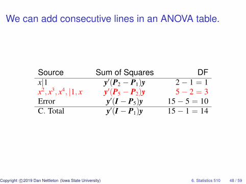
We can add consecutive lines in an ANOVA table.
Source Sum of Squares DFx|1 y′(P2 − P1)y 2− 1 = 1x2, x3, x4, |1, x y′(P5 − P2)y 5− 2 = 3Error y′(I − P5)y 15− 5 = 10C. Total y′(I − P1)y 15− 1 = 14
Copyright c©2019 Dan Nettleton (Iowa State University) 6. Statistics 510 48 / 59
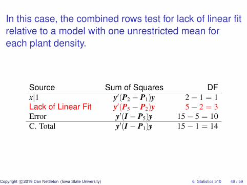
In this case, the combined rows test for lack of linear fitrelative to a model with one unrestricted mean foreach plant density.
Source Sum of Squares DFx|1 y′(P2 − P1)y 2− 1 = 1Lack of Linear Fit y′(P5 − P2)y 5− 2 = 3Error y′(I − P5)y 15− 5 = 10C. Total y′(I − P1)y 15− 1 = 14
Copyright c©2019 Dan Nettleton (Iowa State University) 6. Statistics 510 49 / 59
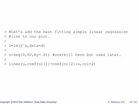
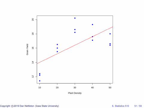
> #Let’s add the best fitting simple linear regression> #line to our plot.>> o=lm(y˜x,data=d)>> u=seq(0,60,by=.01) #overkill here but used later.>> lines(u,coef(o)[1]+coef(o)[2]*u,col=2)
Copyright c©2019 Dan Nettleton (Iowa State University) 6. Statistics 510 50 / 59
●
●
●
●
●
●
●
●
●
●
●
●
●
●●
10 20 30 40 50
1214
1618
20
Plant Density
Gra
in Y
ield
Copyright c©2019 Dan Nettleton (Iowa State University) 6. Statistics 510 51 / 59
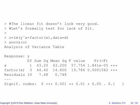
> #The linear fit doesn’t look very good.> #Let’s formally test for lack of fit.>> o=lm(y˜x+factor(x),data=d)> anova(o)Analysis of Variance Table
Response: yDf Sum Sq Mean Sq F value Pr(>F)
x 1 43.20 43.200 57.754 1.841e-05 ***factor(x) 3 44.40 14.800 19.786 0.0001582 ***Residuals 10 7.48 0.748---Signif. codes: 0 *** 0.001 ** 0.01 * 0.05 . 0.1 1
Copyright c©2019 Dan Nettleton (Iowa State University) 6. Statistics 510 52 / 59
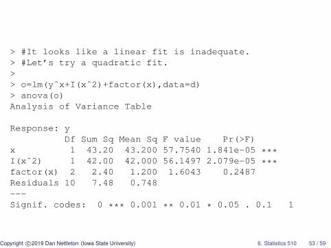
> #It looks like a linear fit is inadequate.> #Let’s try a quadratic fit.>> o=lm(y˜x+I(xˆ2)+factor(x),data=d)> anova(o)Analysis of Variance Table
Response: yDf Sum Sq Mean Sq F value Pr(>F)
x 1 43.20 43.200 57.7540 1.841e-05 ***I(xˆ2) 1 42.00 42.000 56.1497 2.079e-05 ***factor(x) 2 2.40 1.200 1.6043 0.2487Residuals 10 7.48 0.748---Signif. codes: 0 *** 0.001 ** 0.01 * 0.05 . 0.1 1
Copyright c©2019 Dan Nettleton (Iowa State University) 6. Statistics 510 53 / 59
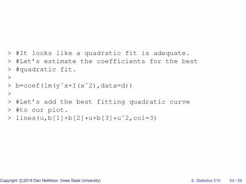
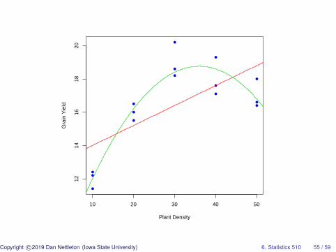
> #It looks like a quadratic fit is adequate.> #Let’s estimate the coefficients for the best> #quadratic fit.>> b=coef(lm(y˜x+I(xˆ2),data=d))>> #Let’s add the best fitting quadratic curve> #to our plot.> lines(u,b[1]+b[2]*u+b[3]*uˆ2,col=3)
Copyright c©2019 Dan Nettleton (Iowa State University) 6. Statistics 510 54 / 59
●
●
●
●
●
●
●
●
●
●
●
●
●
●●
10 20 30 40 50
1214
1618
20
Plant Density
Gra
in Y
ield
Copyright c©2019 Dan Nettleton (Iowa State University) 6. Statistics 510 55 / 59

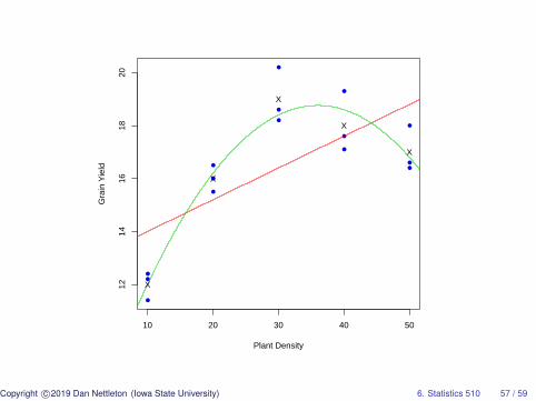
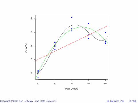
> #Let’s add the treatment group means to our plot.>> trt.means=tapply(d$y,d$x,mean)>> points(unique(d$x),trt.means,pch="X")
Copyright c©2019 Dan Nettleton (Iowa State University) 6. Statistics 510 56 / 59
●
●
●
●
●
●
●
●
●
●
●
●
●
●●
10 20 30 40 50
1214
1618
20
Plant Density
Gra
in Y
ield
X
X
X
X
X
Copyright c©2019 Dan Nettleton (Iowa State University) 6. Statistics 510 57 / 59
> #The quartic fit will pass through the treatment> #means.>>> b=coef(lm(y˜x+I(xˆ2)+I(xˆ3)+I(xˆ4),data=d))> lines(u,b[1]+b[2]*u+b[3]*uˆ2+b[4]*uˆ3+b[5]*uˆ4,col=1)
Copyright c©2019 Dan Nettleton (Iowa State University) 6. Statistics 510 58 / 59
●
●
●
●
●
●
●
●
●
●
●
●
●
●●
10 20 30 40 50
1214
1618
20
Plant Density
Gra
in Y
ield
X
X
X
X
X
Copyright c©2019 Dan Nettleton (Iowa State University) 6. Statistics 510 59 / 59