
Mean-field Methods in Estimation & Control
131
CSL COORDINATED SCIENCE LABORATORY Mean-field Methods in Estimation & Control Prashant G. Mehta Coordinated Science Laboratory Department of Mechanical Science and Engineering University of Illinois at Urbana-Champaign EE Seminar, Harvard Apr. 1, 2011
-
Upload
mehtapgresearch -
Category
Technology
-
view
476 -
download
2
Transcript of Mean-field Methods in Estimation & Control
CSLCOORDINATED SCIENCE LABORATORY
Mean-field Methods in Estimation & Control
Prashant G. Mehta
Coordinated Science LaboratoryDepartment of Mechanical Science and Engineering
University of Illinois at Urbana-Champaign
EE Seminar, HarvardApr. 1, 2011
Introduction Kuramoto model
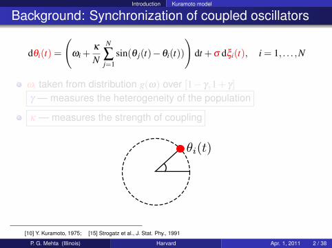
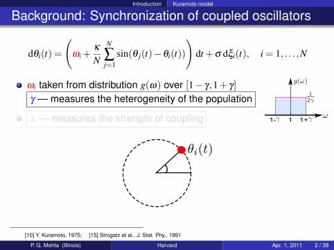
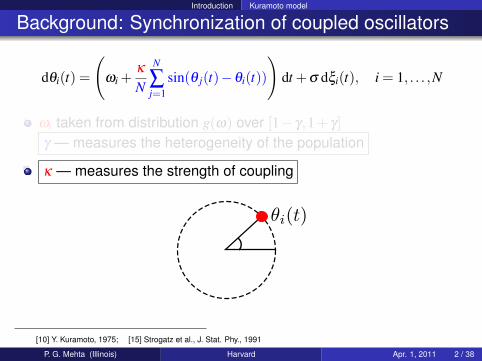
Background: Synchronization of coupled oscillators
dθi(t) =
(ωi +
κ
N
N
∑j=1
sin(θ j(t)−θi(t))
)dt +σ dξi(t), i = 1, . . . ,N
ωi taken from distribution g(ω) over [1− γ,1+ γ]γ — measures the heterogeneity of the population
κ — measures the strength of coupling
[10] Y. Kuramoto, 1975; [15] Strogatz et al., J. Stat. Phy., 1991
P. G. Mehta (Illinois) Harvard Apr. 1, 2011 2 / 38
Introduction Kuramoto model
Background: Synchronization of coupled oscillators
dθi(t) =
(ωi +
κ
N
N
∑j=1
sin(θ j(t)−θi(t))
)dt +σ dξi(t), i = 1, . . . ,N
ωi taken from distribution g(ω) over [1− γ,1+ γ]γ — measures the heterogeneity of the population
κ — measures the strength of coupling 1- 1+1
[10] Y. Kuramoto, 1975; [15] Strogatz et al., J. Stat. Phy., 1991
P. G. Mehta (Illinois) Harvard Apr. 1, 2011 2 / 38
Introduction Kuramoto model
Background: Synchronization of coupled oscillators
dθi(t) =
(ωi +
κ
N
N
∑j=1
sin(θ j(t)−θi(t))
)dt +σ dξi(t), i = 1, . . . ,N
ωi taken from distribution g(ω) over [1− γ,1+ γ]γ — measures the heterogeneity of the population
κ — measures the strength of coupling
[10] Y. Kuramoto, 1975; [15] Strogatz et al., J. Stat. Phy., 1991
P. G. Mehta (Illinois) Harvard Apr. 1, 2011 2 / 38

Introduction Kuramoto model
Background: Synchronization of coupled oscillators
dθi(t) =
(ωi +
κ
N
N
∑j=1
sin(θ j(t)−θi(t))
)dt +σ dξi(t), i = 1, . . . ,N
ωi taken from distribution g(ω) over [1− γ,1+ γ]γ — measures the heterogeneity of the population
κ — measures the strength of coupling
0 0.1 0.20.1
0.15
0.2
0.25
0.3 Locking
Incoherence
κ
κ < κc(γ)
R
γ
Synchrony
Incoherence
[10] Y. Kuramoto, 1975; [15] Strogatz et al., J. Stat. Phy., 1991
P. G. Mehta (Illinois) Harvard Apr. 1, 2011 2 / 38
Introduction Kuramoto model
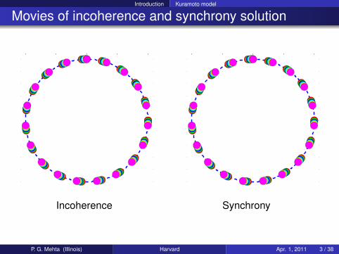
Movies of incoherence and synchrony solution
−1
0.8
0.6
0.4
0.2
0
0.2
0.4
0.6
0.8
1
−1
0.8
0.6
0.4
0.2
0
0.2
0.4
0.6
0.8
1
Incoherence Synchrony
P. G. Mehta (Illinois) Harvard Apr. 1, 2011 3 / 38
Introduction Oscillator examples
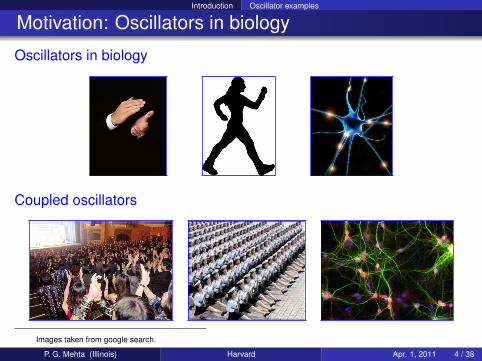
Motivation: Oscillators in biology
Oscillators in biology
Coupled oscillators
Images taken from google search.
P. G. Mehta (Illinois) Harvard Apr. 1, 2011 4 / 38
Introduction Oscillator examples
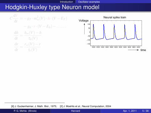
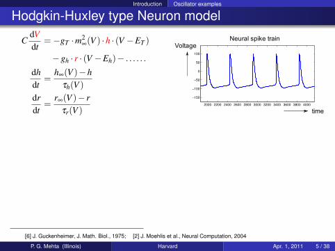
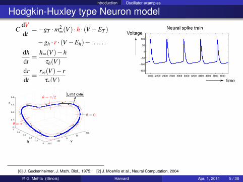
Hodgkin-Huxley type Neuron model
CdVdt
=−gT ·m2∞(V ) ·h · (V −ET )
−gh · r · (V −Eh)− . . . . . .
dhdt
=h∞(V )−h
τh(V )drdt
=r∞(V )− r
τr(V )2000 2200 2400 2600 2800 3000 3200 3400 3600 3800 4000
−150
−100
−50
0
50
100
Voltage
time
Neural spike train
[6] J. Guckenheimer, J. Math. Biol., 1975; [2] J. Moehlis et al., Neural Computation, 2004
P. G. Mehta (Illinois) Harvard Apr. 1, 2011 5 / 38
Introduction Oscillator examples
Hodgkin-Huxley type Neuron model
CdVdt
=−gT ·m2∞(V ) ·h · (V −ET )
−gh · r · (V −Eh)− . . . . . .
dhdt
=h∞(V )−h
τh(V )drdt
=r∞(V )− r
τr(V )2000 2200 2400 2600 2800 3000 3200 3400 3600 3800 4000
−150
−100
−50
0
50
100
Voltage
time
Neural spike train
−100
−50
0
50
100
0
0.2
0.4
0.6
0.8
10
0.1
0.2
0.3
0.4
Vh
r
Limit cyle
r
h v
[6] J. Guckenheimer, J. Math. Biol., 1975; [2] J. Moehlis et al., Neural Computation, 2004
P. G. Mehta (Illinois) Harvard Apr. 1, 2011 5 / 38
Introduction Oscillator examples
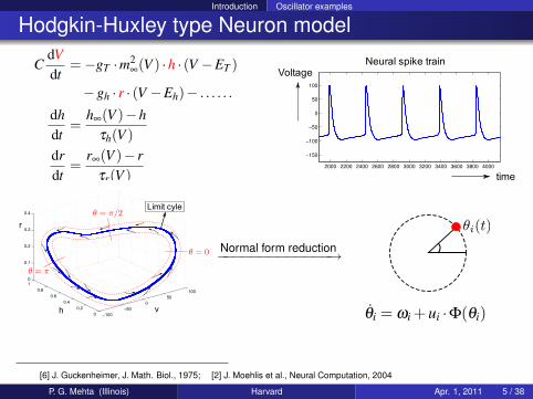
Hodgkin-Huxley type Neuron model
CdVdt
=−gT ·m2∞(V ) ·h · (V −ET )
−gh · r · (V −Eh)− . . . . . .
dhdt
=h∞(V )−h
τh(V )drdt
=r∞(V )− r
τr(V )2000 2200 2400 2600 2800 3000 3200 3400 3600 3800 4000
−150
−100
−50
0
50
100
Voltage
time
Neural spike train
−100
−50
0
50
100
0
0.2
0.4
0.6
0.8
10
0.1
0.2
0.3
0.4
Vh
r
Limit cyle
r
h v
Normal form reduction−−−−−−−−−−−−−→
θi = ωi +ui ·Φ(θi)
[6] J. Guckenheimer, J. Math. Biol., 1975; [2] J. Moehlis et al., Neural Computation, 2004
P. G. Mehta (Illinois) Harvard Apr. 1, 2011 5 / 38

Introduction Role of Neural Rhythms
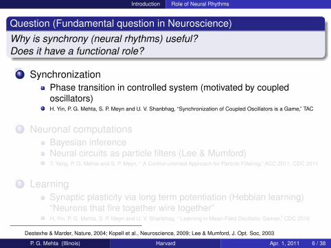
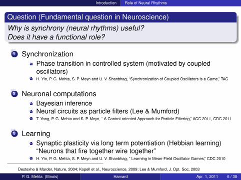
Question (Fundamental question in Neuroscience)Why is synchrony (neural rhythms) useful?Does it have a functional role?
1 SynchronizationPhase transition in controlled system (motivated by coupledoscillators)H. Yin, P. G. Mehta, S. P. Meyn and U. V. Shanbhag, “Synchronization of Coupled Oscillators is a Game,” TAC
2 Neuronal computationsBayesian inferenceNeural circuits as particle filters (Lee & Mumford)T. Yang, P. G. Mehta and S. P. Meyn, “ A Control-oriented Approach for Particle Filtering,” ACC 2011, CDC 2011
3 LearningSynaptic plasticity via long term potentiation (Hebbian learning)“Neurons that fire together wire together”H. Yin, P. G. Mehta, S. P. Meyn and U. V. Shanbhag, “ Learning in Mean-Field Oscillator Games,” CDC 2010
Destexhe & Marder, Nature, 2004; Kopell et al., Neuroscience, 2009; Lee & Mumford, J. Opt. Soc, 2003
P. G. Mehta (Illinois) Harvard Apr. 1, 2011 6 / 38
Introduction Role of Neural Rhythms
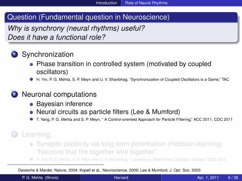
Question (Fundamental question in Neuroscience)Why is synchrony (neural rhythms) useful?Does it have a functional role?
1 SynchronizationPhase transition in controlled system (motivated by coupledoscillators)H. Yin, P. G. Mehta, S. P. Meyn and U. V. Shanbhag, “Synchronization of Coupled Oscillators is a Game,” TAC
2 Neuronal computationsBayesian inferenceNeural circuits as particle filters (Lee & Mumford)T. Yang, P. G. Mehta and S. P. Meyn, “ A Control-oriented Approach for Particle Filtering,” ACC 2011, CDC 2011
3 LearningSynaptic plasticity via long term potentiation (Hebbian learning)“Neurons that fire together wire together”H. Yin, P. G. Mehta, S. P. Meyn and U. V. Shanbhag, “ Learning in Mean-Field Oscillator Games,” CDC 2010
Destexhe & Marder, Nature, 2004; Kopell et al., Neuroscience, 2009; Lee & Mumford, J. Opt. Soc, 2003
P. G. Mehta (Illinois) Harvard Apr. 1, 2011 6 / 38

Part I
Mean-field Control
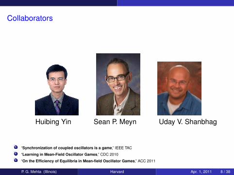
Collaborators
Huibing Yin Sean P. Meyn Uday V. Shanbhag
“Synchronization of coupled oscillators is a game,” IEEE TAC
“Learning in Mean-Field Oscillator Games,” CDC 2010
“On the Efficiency of Equilibria in Mean-field Oscillator Games,” ACC 2011
P. G. Mehta (Illinois) Harvard Apr. 1, 2011 8 / 38
Derivation of model Problem statement
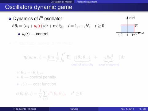
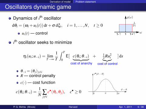
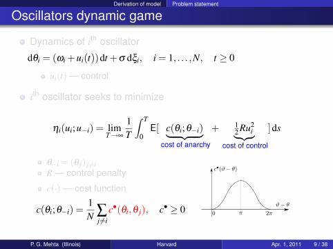
Oscillators dynamic game
Dynamics of ith oscillator
dθi = (ωi +ui(t))dt +σ dξi, i = 1, . . . ,N, t ≥ 0
ui(t) — control 1- 1+1
ith oscillator seeks to minimize
ηi(ui;u−i) = limT→∞
1T
∫ T
0E[ c(θi;θ−i)︸ ︷︷ ︸
cost of anarchy
+ 12 Ru2
i︸ ︷︷ ︸cost of control
]ds
θ−i = (θ j) j 6=iR — control penalty
c(·) — cost function
c(θi;θ−i) =1N ∑
j 6=ic•(θi,θ j), c• ≥ 0
P. G. Mehta (Illinois) Harvard Apr. 1, 2011 9 / 38
Derivation of model Problem statement
Oscillators dynamic game
Dynamics of ith oscillator
dθi = (ωi +ui(t))dt +σ dξi, i = 1, . . . ,N, t ≥ 0
ui(t) — control
ith oscillator seeks to minimize
ηi(ui;u−i) = limT→∞
1T
∫ T
0E[ c(θi;θ−i)︸ ︷︷ ︸
cost of anarchy
+ 12 Ru2
i︸ ︷︷ ︸cost of control
]ds
θ−i = (θ j) j 6=iR — control penalty
c(·) — cost function
c(θi;θ−i) =1N ∑
j 6=ic•(θi,θ j), c• ≥ 0
P. G. Mehta (Illinois) Harvard Apr. 1, 2011 9 / 38
Derivation of model Mean-field model
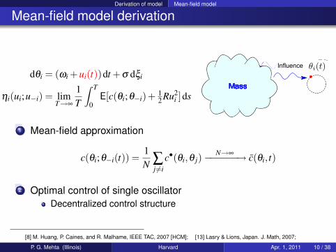
Mean-field model derivation
dθi = (ωi +ui(t))dt +σ dξi
ηi(ui;u−i) = limT→∞
1T
∫ T
0E[c(θi;θ−i)+ 1
2 Ru2i ]ds
Influence
Influence
Mass
1 Mean-field approximation
c(θi;θ−i(t)) =1N ∑
j 6=ic•(θi,θ j)
N→∞−−−−−−→ c(θi, t)
2 Optimal control of single oscillatorDecentralized control structure
[8] M. Huang, P. Caines, and R. Malhame, IEEE TAC, 2007 [HCM]; [13] Lasry & Lions, Japan. J. Math, 2007;
P. G. Mehta (Illinois) Harvard Apr. 1, 2011 10 / 38
Derivation of model Derivation steps
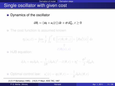
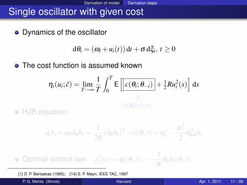
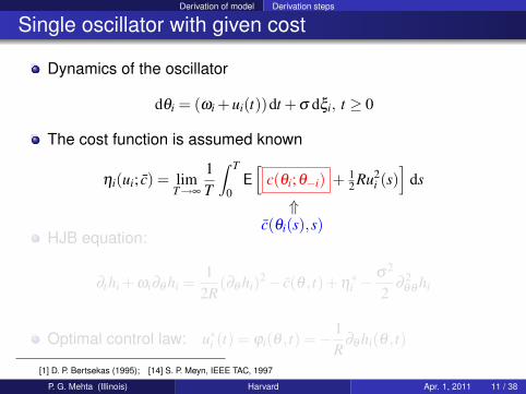
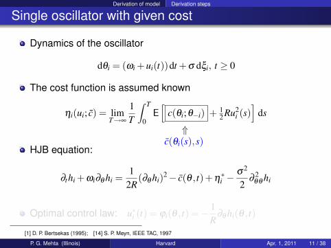
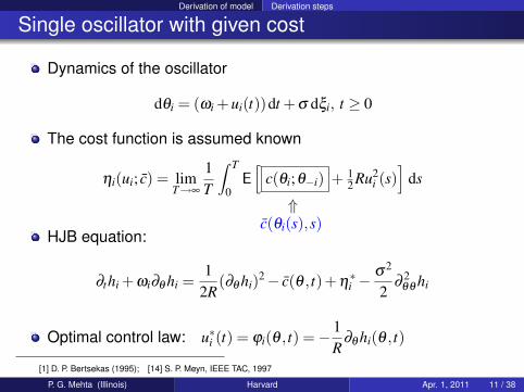
Single oscillator with given cost
Dynamics of the oscillator
dθi = (ωi +ui(t))dt +σ dξi, t ≥ 0
The cost function is assumed known
ηi(ui; c) = limT→∞
1T
∫ T
0E[
c(θi;θ−i) + 12 Ru2
i (s)]
ds
⇑c(θi(s),s)
HJB equation:
∂thi +ωi∂θ hi =1
2R(∂θ hi)2− c(θ , t)+η
∗i −
σ2
2∂
2θθ hi
Optimal control law: u∗i (t) = ϕi(θ , t) =− 1R
∂θ hi(θ , t)
[1] D. P. Bertsekas (1995); [14] S. P. Meyn, IEEE TAC, 1997
P. G. Mehta (Illinois) Harvard Apr. 1, 2011 11 / 38
Derivation of model Derivation steps
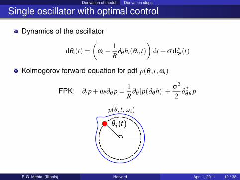
Single oscillator with optimal control
Dynamics of the oscillator
dθi(t) =(
ωi−1R
∂θ hi(θi, t))
dt +σ dξi(t)
Kolmogorov forward equation for pdf p(θ , t,ωi)
FPK: ∂t p+ωi∂θ p =1R
∂θ [p(∂θ h)]+σ2
2∂
2θθ p
P. G. Mehta (Illinois) Harvard Apr. 1, 2011 12 / 38
Derivation of model Derivation steps
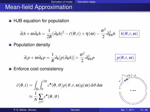
Mean-field Approximation
HJB equation for population
∂th+ω∂θ h =1
2R(∂θ h)2− c(θ , t)+η(ω)− σ2
2∂
2θθ h h(θ , t,ω)
Population density
∂t p+ω∂θ p =1R
∂θ [p(∂θ h)]+σ2
2∂
2θθ p p(θ , t,ω)
Enforce cost consistency
c(θ , t) =∫
Ω
∫ 2π
0c•(θ ,ϑ)p(ϑ , t,ω)g(ω)dϑ dω
≈ 1N ∑
j 6=ic•(θ ,ϑ)
P. G. Mehta (Illinois) Harvard Apr. 1, 2011 13 / 38
Derivation of model Derivation steps
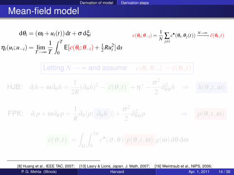
Mean-field model
dθi = (ωi +ui(t))dt +σ dξi
ηi(ui;u−i) = limT→∞
1T
∫ T
0E[c(θi;θ−i)+ 1
2 Ru2i ]ds
c(θi;θ−i) =1N ∑
j 6=ic•(θi,θ j(t))
N→∞−−−→ c(θi, t)
Letting N→ ∞ and assume c(θi,θ−i)→ c(θi, t)
HJB: ∂th+ω∂θ h =1
2R(∂θ h)2− c(θ , t) +η
∗− σ2
2∂
2θθ h ⇒ h(θ , t,ω)
FPK: ∂t p+ω∂θ p =1R
∂θ [p( ∂θ h )]+σ2
2∂
2θθ p ⇒ p(θ , t,ω)
c(ϑ , t) =∫
Ω
∫ 2π
0c•(ϑ ,θ) p(θ , t,ω) g(ω)dθ dω
[8] Huang et al., IEEE TAC, 2007; [13] Lasry & Lions, Japan. J. Math, 2007; [16] Weintraub et al., NIPS, 2006;P. G. Mehta (Illinois) Harvard Apr. 1, 2011 14 / 38
Derivation of model Derivation steps
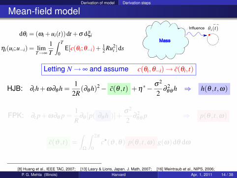
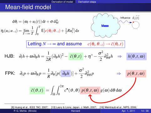
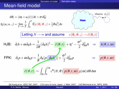
Mean-field model
dθi = (ωi +ui(t))dt +σ dξi
ηi(ui;u−i) = limT→∞
1T
∫ T
0E[c(θi;θ−i)+ 1
2 Ru2i ]ds
Influence
Influence
Mass
Letting N→ ∞ and assume c(θi,θ−i)→ c(θi, t)
HJB: ∂th+ω∂θ h =1
2R(∂θ h)2− c(θ , t) +η
∗− σ2
2∂
2θθ h ⇒ h(θ , t,ω)
FPK: ∂t p+ω∂θ p =1R
∂θ [p( ∂θ h )]+σ2
2∂
2θθ p ⇒ p(θ , t,ω)
c(ϑ , t) =∫
Ω
∫ 2π
0c•(ϑ ,θ) p(θ , t,ω) g(ω)dθ dω
[8] Huang et al., IEEE TAC, 2007; [13] Lasry & Lions, Japan. J. Math, 2007; [16] Weintraub et al., NIPS, 2006;P. G. Mehta (Illinois) Harvard Apr. 1, 2011 14 / 38
Derivation of model Derivation steps
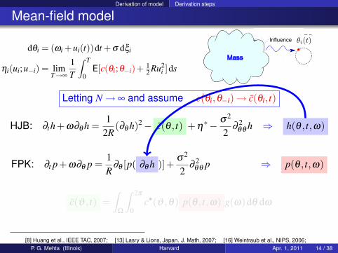
Mean-field model
dθi = (ωi +ui(t))dt +σ dξi
ηi(ui;u−i) = limT→∞
1T
∫ T
0E[c(θi;θ−i)+ 1
2 Ru2i ]ds
Influence
Influence
Mass
Letting N→ ∞ and assume c(θi,θ−i)→ c(θi, t)
HJB: ∂th+ω∂θ h =1
2R(∂θ h)2− c(θ , t) +η
∗− σ2
2∂
2θθ h ⇒ h(θ , t,ω)
FPK: ∂t p+ω∂θ p =1R
∂θ [p( ∂θ h )]+σ2
2∂
2θθ p ⇒ p(θ , t,ω)
c(ϑ , t) =∫
Ω
∫ 2π
0c•(ϑ ,θ) p(θ , t,ω) g(ω)dθ dω
[8] Huang et al., IEEE TAC, 2007; [13] Lasry & Lions, Japan. J. Math, 2007; [16] Weintraub et al., NIPS, 2006;P. G. Mehta (Illinois) Harvard Apr. 1, 2011 14 / 38
Solutions of PDE model ε-Nash equilibrium
Solution of PDEs gives ε-Nash equilibrium
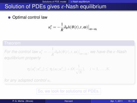
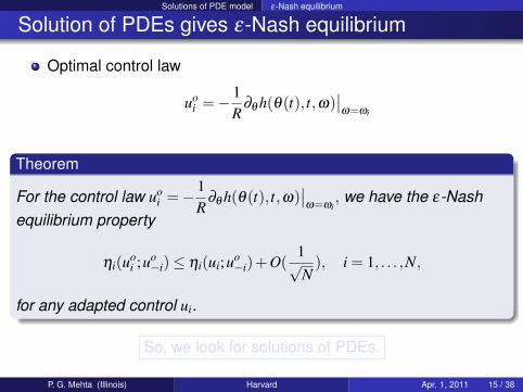
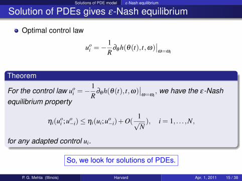
Optimal control law
uoi =− 1
R∂θ h(θ(t), t,ω)
∣∣ω=ωi
Theorem
For the control law uoi =− 1
R∂θ h(θ(t), t,ω)
∣∣ω=ωi
, we have the ε-Nashequilibrium property
ηi(uoi ;uo−i)≤ ηi(ui;uo
−i)+O(1√N
), i = 1, . . . ,N,
for any adapted control ui.
So, we look for solutions of PDEs.
P. G. Mehta (Illinois) Harvard Apr. 1, 2011 15 / 38
Solutions of PDE model ε-Nash equilibrium
Solution of PDEs gives ε-Nash equilibrium
Optimal control law
uoi =− 1
R∂θ h(θ(t), t,ω)
∣∣ω=ωi
Theorem
For the control law uoi =− 1
R∂θ h(θ(t), t,ω)
∣∣ω=ωi
, we have the ε-Nashequilibrium property
ηi(uoi ;uo−i)≤ ηi(ui;uo
−i)+O(1√N
), i = 1, . . . ,N,
for any adapted control ui.
So, we look for solutions of PDEs.
P. G. Mehta (Illinois) Harvard Apr. 1, 2011 15 / 38
Solutions of PDE model Synchronization
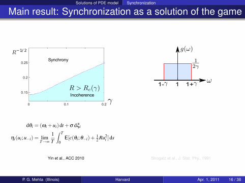
Main result: Synchronization as a solution of the game
Locking
0 0.1 0.2
0.15
0.2
0.25
R−1/ 2
γγIncoherence
R > Rc(γ)
Synchrony
Incoherence
dθi = (ωi +ui)dt +σ dξi
ηi(ui;u−i) = limT→∞
1T
∫ T
0E[c(θi;θ−i)+ 1
2 Ru2i ]ds
1- 1+1
Yin et al., ACC 2010 Strogatz et al., J. Stat. Phy., 1991
P. G. Mehta (Illinois) Harvard Apr. 1, 2011 16 / 38
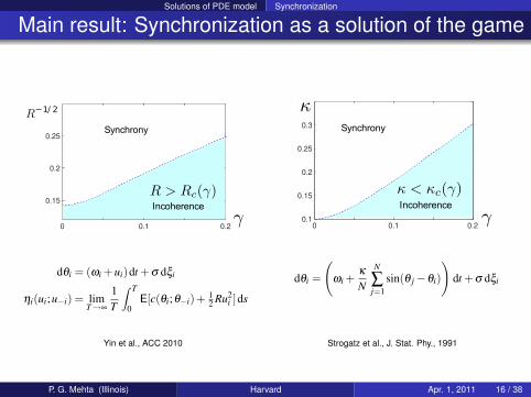
Solutions of PDE model Synchronization
Main result: Synchronization as a solution of the game
Locking
0 0.1 0.2
0.15
0.2
0.25
R−1/ 2
γγIncoherence
R > Rc(γ)
Synchrony
Incoherence
dθi = (ωi +ui)dt +σ dξi
ηi(ui;u−i) = limT→∞
1T
∫ T
0E[c(θi;θ−i)+ 1
2 Ru2i ]ds
0 0.1 0.20.1
0.15
0.2
0.25
0.3 Locking
Incoherence
κ
κ < κc(γ)
R
γ
Synchrony
Incoherence
dθi =
(ωi +
κ
N
N
∑j=1
sin(θ j−θi)
)dt +σ dξi
Yin et al., ACC 2010 Strogatz et al., J. Stat. Phy., 1991
P. G. Mehta (Illinois) Harvard Apr. 1, 2011 16 / 38
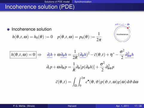
Solutions of PDE model Synchronization
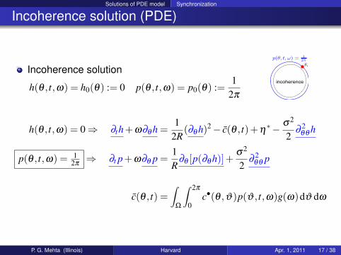
Incoherence solution (PDE)
Incoherence solution
h(θ , t,ω) = h0(θ) := 0 p(θ , t,ω) = p0(θ) :=1
2π
h(θ , t,ω) = 0 ⇒ ∂th+ω∂θ h =1
2R(∂θ h)2− c(θ , t)+η
∗− σ2
2∂
2θθ h
∂t p+ω∂θ p =1R
∂θ [p(∂θ h)]+σ2
2∂
2θθ p
c(θ , t) =∫
Ω
∫ 2π
0c•(θ ,ϑ)p(ϑ , t,ω)g(ω)dϑ dω
P. G. Mehta (Illinois) Harvard Apr. 1, 2011 17 / 38
Solutions of PDE model Synchronization
Incoherence solution (PDE)
Incoherence solution
h(θ , t,ω) = h0(θ) := 0 p(θ , t,ω) = p0(θ) :=1
2π
h(θ , t,ω) = 0⇒ ∂th+ω∂θ h =1
2R(∂θ h)2− c(θ , t)+η
∗− σ2
2∂
2θθ h
p(θ , t,ω) = 12π⇒ ∂t p+ω∂θ p =
1R
∂θ [p(∂θ h)]+σ2
2∂
2θθ p
c(θ , t) =∫
Ω
∫ 2π
0c•(θ ,ϑ)p(ϑ , t,ω)g(ω)dϑ dω
P. G. Mehta (Illinois) Harvard Apr. 1, 2011 17 / 38
Solutions of PDE model Synchronization
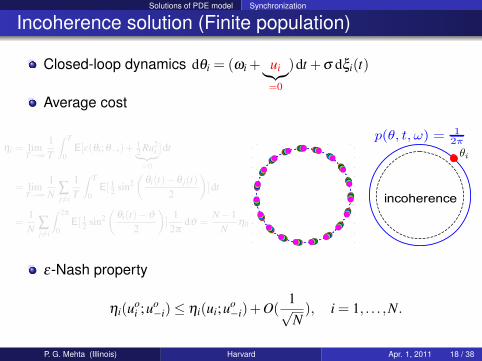
Incoherence solution (Finite population)
Closed-loop dynamics dθi = (ωi + ui︸︷︷︸=0
)dt +σ dξi(t)
Average cost
ηi = limT→∞
1T
∫ T
0E[c(θi;θ−i)+ 1
2 Ru2i︸ ︷︷ ︸
=0
]dt
= limT→∞
1N ∑
j 6=i
1T
∫ T
0E[ 1
2 sin2(
θi(t)−θ j(t)2
)]dt
=1N ∑
j 6=i
∫ 2π
0E[ 1
2 sin2(
θi(t)−ϑ
2
)]
12π
dϑ =N−1
Nη0
−1
0.8
0.6
0.4
0.2
0
0.2
0.4
0.6
0.8
1
ε-Nash property
ηi(uoi ;uo−i)≤ ηi(ui;uo
−i)+O(1√N
), i = 1, . . . ,N.
P. G. Mehta (Illinois) Harvard Apr. 1, 2011 18 / 38
Solutions of PDE model Synchronization
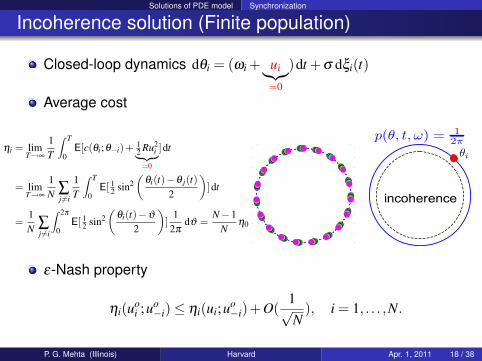
Incoherence solution (Finite population)
Closed-loop dynamics dθi = (ωi + ui︸︷︷︸=0
)dt +σ dξi(t)
Average cost
ηi = limT→∞
1T
∫ T
0E[c(θi;θ−i)+ 1
2 Ru2i︸ ︷︷ ︸
=0
]dt
= limT→∞
1N ∑
j 6=i
1T
∫ T
0E[ 1
2 sin2(
θi(t)−θ j(t)2
)]dt
=1N ∑
j 6=i
∫ 2π
0E[ 1
2 sin2(
θi(t)−ϑ
2
)]
12π
dϑ =N−1
Nη0
−1
0.8
0.6
0.4
0.2
0
0.2
0.4
0.6
0.8
1
ε-Nash property
ηi(uoi ;uo−i)≤ ηi(ui;uo
−i)+O(1√N
), i = 1, . . . ,N.
P. G. Mehta (Illinois) Harvard Apr. 1, 2011 18 / 38
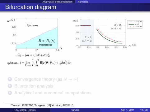
Analysis of phase transition Numerics
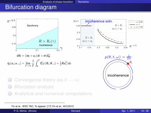
Bifurcation diagram
Locking
0 0.1 0.2
0.15
0.2
0.25
R−1/ 2
γγIncoherence
R > Rc(γ)
Synchrony
Incoherence R−1/2
η(ω)
0. 1 0.15 0. 2 0.25 0. 3 0.35
0. 1
0.15
0. 2
0.25
ω = 0.95
ω = 1
ω = 1.05
R > Rc
η(ω) = η0
R < Rc
η(ω) < η0
dθi = (ωi +ui)dt +σ dξi
ηi(ui;u−i) = limT→∞
1T
∫ T
0E[c(θi;θ−i)+ 1
2 Ru2i ]ds
1 Convergence theory (as N→ ∞)2 Bifurcation analysis3 Analytical and numerical computations
Yin et al., IEEE TAC, To appear; [17] Yin et al., ACC2010
P. G. Mehta (Illinois) Harvard Apr. 1, 2011 19 / 38
Analysis of phase transition Numerics
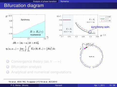
Bifurcation diagram
Locking
0 0.1 0.2
0.15
0.2
0.25
R−1/ 2
γγIncoherence
R > Rc(γ)
Synchrony
Incoherence R−1/2
η(ω)
0. 1 0.15 0. 2 0.25 0. 3 0.35
0. 1
0.15
0. 2
0.25
ω = 0.95
ω = 1
ω = 1.05
R > Rc
η(ω) = η0
R < Rc
η(ω) < η0
incoherence soln.
dθi = (ωi +ui)dt +σ dξi
ηi(ui;u−i) = limT→∞
1T
∫ T
0E[c(θi;θ−i)+ 1
2 Ru2i ]ds
1 Convergence theory (as N→ ∞)2 Bifurcation analysis3 Analytical and numerical computations
Yin et al., IEEE TAC, To appear; [17] Yin et al., ACC2010
P. G. Mehta (Illinois) Harvard Apr. 1, 2011 19 / 38
Analysis of phase transition Numerics
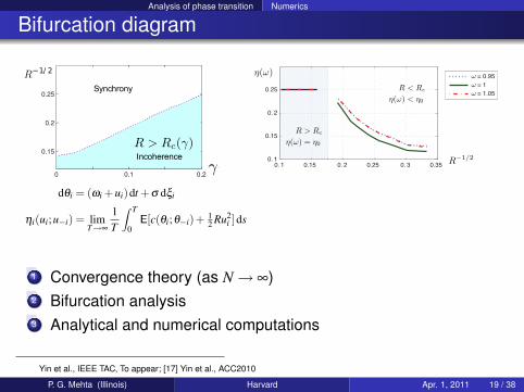
Bifurcation diagram
Locking
0 0.1 0.2
0.15
0.2
0.25
R−1/ 2
γγIncoherence
R > Rc(γ)
Synchrony
Incoherence R−1/2
η(ω)
0. 1 0.15 0. 2 0.25 0. 3 0.35
0. 1
0.15
0. 2
0.25
ω = 0.95
ω = 1
ω = 1.05
R > Rc
η(ω) = η0
R < Rc
η(ω) < η0
synchrony soln.
dθi = (ωi +ui)dt +σ dξi
ηi(ui;u−i) = limT→∞
1T
∫ T
0E[c(θi;θ−i)+ 1
2 Ru2i ]ds
1 Convergence theory (as N→ ∞)2 Bifurcation analysis3 Analytical and numerical computations
Yin et al., IEEE TAC, To appear; [17] Yin et al., ACC2010
P. G. Mehta (Illinois) Harvard Apr. 1, 2011 19 / 38
Analysis of phase transition Numerics
Bifurcation diagram
Locking
0 0.1 0.2
0.15
0.2
0.25
R−1/ 2
γγIncoherence
R > Rc(γ)
Synchrony
Incoherence R−1/2
η(ω)
0. 1 0.15 0. 2 0.25 0. 3 0.35
0. 1
0.15
0. 2
0.25
ω = 0.95
ω = 1
ω = 1.05
R > Rc
η(ω) = η0
R < Rc
η(ω) < η0
dθi = (ωi +ui)dt +σ dξi
ηi(ui;u−i) = limT→∞
1T
∫ T
0E[c(θi;θ−i)+ 1
2 Ru2i ]ds
1 Convergence theory (as N→ ∞)2 Bifurcation analysis3 Analytical and numerical computations
Yin et al., IEEE TAC, To appear; [17] Yin et al., ACC2010
P. G. Mehta (Illinois) Harvard Apr. 1, 2011 19 / 38
Part II
Mean-field Estimation

Collaborators
Tao Yang Sean P. Meyn
“A Control-oriented Approach for Particle Filtering,” ACC 2011
“Feedback Particle Filter with Mean-field Coupling,” submitted to CDC 2011
P. G. Mehta (Illinois) Harvard Apr. 1, 2011 21 / 38
Problem Definition
Filtering problem
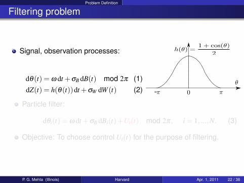
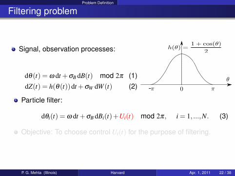
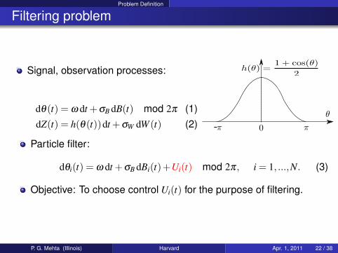
Signal, observation processes:
dθ(t) = ω dt +σB dB(t) mod 2π (1)dZ(t) = h(θ(t))dt +σW dW (t) (2) -
Particle filter:
dθi(t) = ω dt +σB dBi(t)+Ui(t) mod 2π, i = 1, ...,N. (3)
Objective: To choose control Ui(t) for the purpose of filtering.
P. G. Mehta (Illinois) Harvard Apr. 1, 2011 22 / 38
Problem Definition
Filtering problem
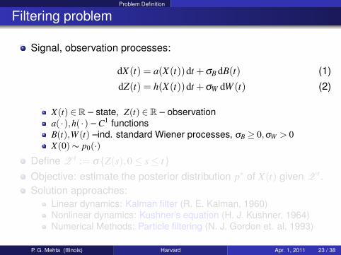
Signal, observation processes:
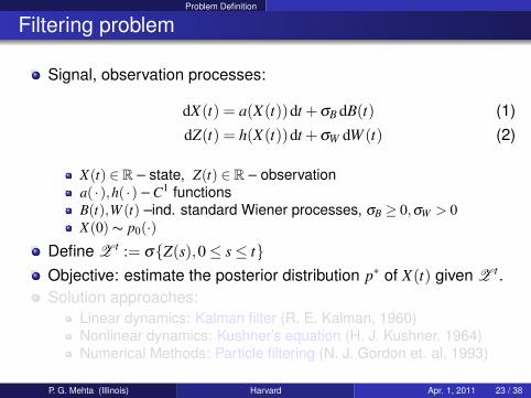
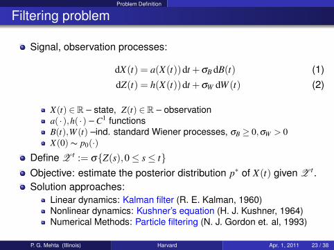
dX(t) = a(X(t))dt +σB dB(t) (1)dZ(t) = h(X(t))dt +σW dW (t) (2)
X(t) ∈ R – state, Z(t) ∈ R – observationa( ·),h( ·) – C1 functionsB(t),W (t) –ind. standard Wiener processes, σB ≥ 0,σW > 0X(0) ∼ p0(·)
Define Z t := σZ(s),0≤ s≤ tObjective: estimate the posterior distribution p∗ of X(t) given Z t .Solution approaches:
Linear dynamics: Kalman filter (R. E. Kalman, 1960)Nonlinear dynamics: Kushner’s equation (H. J. Kushner, 1964)Numerical Methods: Particle filtering (N. J. Gordon et. al, 1993)
P. G. Mehta (Illinois) Harvard Apr. 1, 2011 23 / 38
Problem Definition
Filtering problem
Signal, observation processes:
dX(t) = a(X(t))dt +σB dB(t) (1)dZ(t) = h(X(t))dt +σW dW (t) (2)
X(t) ∈ R – state, Z(t) ∈ R – observationa( ·),h( ·) – C1 functionsB(t),W (t) –ind. standard Wiener processes, σB ≥ 0,σW > 0X(0) ∼ p0(·)
Define Z t := σZ(s),0≤ s≤ tObjective: estimate the posterior distribution p∗ of X(t) given Z t .Solution approaches:
Linear dynamics: Kalman filter (R. E. Kalman, 1960)Nonlinear dynamics: Kushner’s equation (H. J. Kushner, 1964)Numerical Methods: Particle filtering (N. J. Gordon et. al, 1993)
P. G. Mehta (Illinois) Harvard Apr. 1, 2011 23 / 38
Existing Approach Kalman Filter
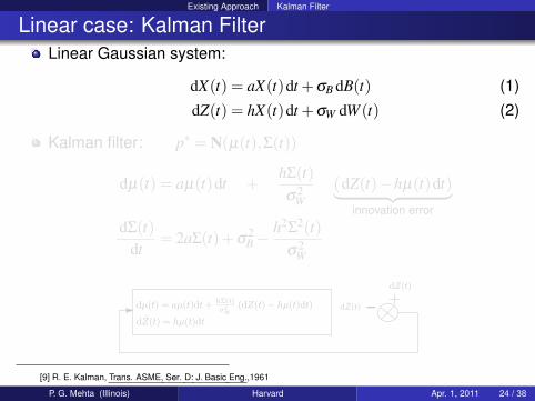
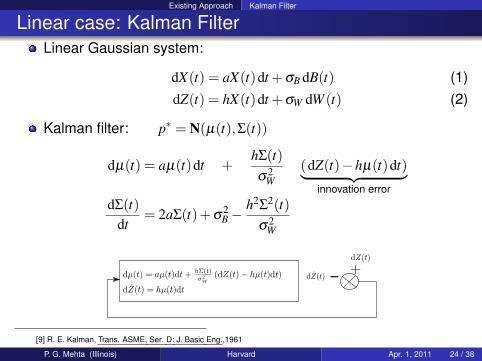
Linear case: Kalman FilterLinear Gaussian system:
dX(t) = aX(t)dt +σB dB(t) (1)dZ(t) = hX(t)dt +σW dW (t) (2)
Kalman filter: p∗ = N(µ(t),Σ(t))
dµ(t) = aµ(t)dt +hΣ(t)σ2
W(dZ(t)−hµ(t)dt)︸ ︷︷ ︸
innovation error
dΣ(t)dt
= 2aΣ(t)+σ2B−
h2Σ2(t)σ2
W
[9] R. E. Kalman, Trans. ASME, Ser. D: J. Basic Eng.,1961
P. G. Mehta (Illinois) Harvard Apr. 1, 2011 24 / 38
Existing Approach Kalman Filter
Linear case: Kalman FilterLinear Gaussian system:
dX(t) = aX(t)dt +σB dB(t) (1)dZ(t) = hX(t)dt +σW dW (t) (2)
Kalman filter: p∗ = N(µ(t),Σ(t))
dµ(t) = aµ(t)dt +hΣ(t)σ2
W(dZ(t)−hµ(t)dt)︸ ︷︷ ︸
innovation error
dΣ(t)dt
= 2aΣ(t)+σ2B−
h2Σ2(t)σ2
W
[9] R. E. Kalman, Trans. ASME, Ser. D: J. Basic Eng.,1961
P. G. Mehta (Illinois) Harvard Apr. 1, 2011 24 / 38
Existing Approach Nonlinear case: Kushner’s equation
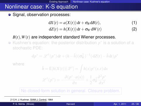
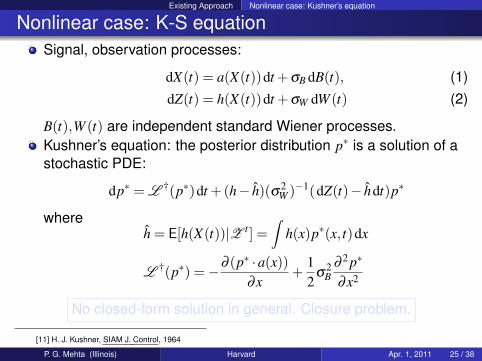
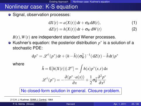
Nonlinear case: K-S equationSignal, observation processes:
dX(t) = a(X(t))dt +σB dB(t), (1)dZ(t) = h(X(t))dt +σW dW (t) (2)
B(t),W (t) are independent standard Wiener processes.Kushner’s equation: the posterior distribution p∗ is a solution of astochastic PDE:
dp∗ = L †(p∗)dt +(h− h)(σ2W )−1(dZ(t)− hdt)p∗
whereh = E[h(X(t))|Z t ] =
∫h(x)p∗(x, t)dx
L †(p∗) =−∂ (p∗ ·a(x))∂x
+12
σ2B
∂ 2 p∗
∂x2
No closed-form solution in general. Closure problem.
[11] H. J. Kushner, SIAM J. Control, 1964
P. G. Mehta (Illinois) Harvard Apr. 1, 2011 25 / 38
Existing Approach Nonlinear case: Kushner’s equation
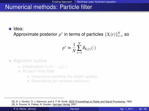
Numerical methods: Particle filter
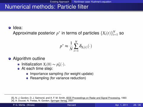
Idea:Approximate posterior p∗ in terms of particles Xi(t)N
i=1 so
p∗ ≈1N
N
∑i=1
δXi(t)(·)
Algorithm outlineInitialization Xi(0) ∼ p∗0(·).At each time step:
Importance sampling (for weight update)Resampling (for variance reduction)
[5], N. J. Gordon, D. J. Salmond, and A. F. M. Smith, IEEE Proceedings on Radar and Signal Processing, 1993[4], A. Doucet, N. Freitas, N. Gordon, Springer-Verlag, 2001
P. G. Mehta (Illinois) Harvard Apr. 1, 2011 26 / 38
Existing Approach Nonlinear case: Kushner’s equation
Numerical methods: Particle filter
Idea:Approximate posterior p∗ in terms of particles Xi(t)N
i=1 so
p∗ ≈1N
N
∑i=1
δXi(t)(·)
Algorithm outlineInitialization Xi(0) ∼ p∗0(·).At each time step:
Importance sampling (for weight update)Resampling (for variance reduction)
[5], N. J. Gordon, D. J. Salmond, and A. F. M. Smith, IEEE Proceedings on Radar and Signal Processing, 1993[4], A. Doucet, N. Freitas, N. Gordon, Springer-Verlag, 2001
P. G. Mehta (Illinois) Harvard Apr. 1, 2011 26 / 38
A Control-Oriented Approach to Particle Filtering Overview
Mean-field filtering
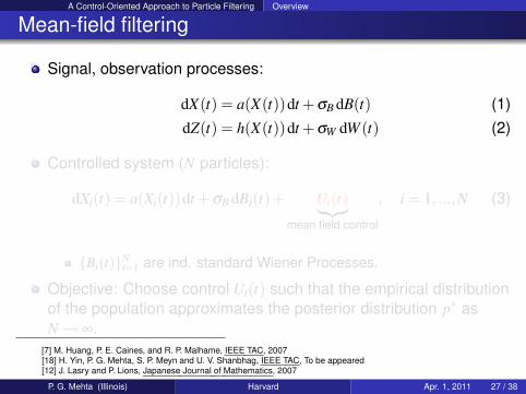
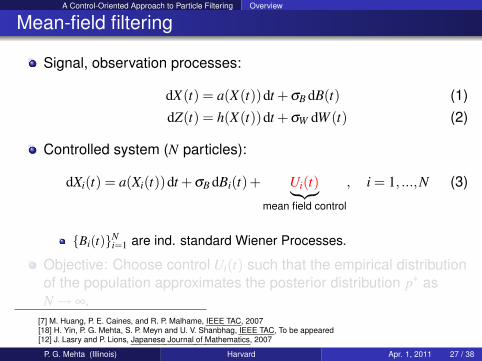
Signal, observation processes:
dX(t) = a(X(t))dt +σB dB(t) (1)dZ(t) = h(X(t))dt +σW dW (t) (2)
Controlled system (N particles):
dXi(t) = a(Xi(t))dt +σB dBi(t)+ Ui(t)︸︷︷︸mean field control
, i = 1, ...,N (3)
Bi(t)Ni=1 are ind. standard Wiener Processes.
Objective: Choose control Ui(t) such that the empirical distributionof the population approximates the posterior distribution p∗ asN→ ∞.
[7] M. Huang, P. E. Caines, and R. P. Malhame, IEEE TAC, 2007[18] H. Yin, P. G. Mehta, S. P. Meyn and U. V. Shanbhag, IEEE TAC, To be appeared[12] J. Lasry and P. Lions, Japanese Journal of Mathematics, 2007
P. G. Mehta (Illinois) Harvard Apr. 1, 2011 27 / 38
A Control-Oriented Approach to Particle Filtering Overview
Mean-field filtering
Signal, observation processes:
dX(t) = a(X(t))dt +σB dB(t) (1)dZ(t) = h(X(t))dt +σW dW (t) (2)
Controlled system (N particles):
dXi(t) = a(Xi(t))dt +σB dBi(t)+ Ui(t)︸︷︷︸mean field control
, i = 1, ...,N (3)
Bi(t)Ni=1 are ind. standard Wiener Processes.
Objective: Choose control Ui(t) such that the empirical distributionof the population approximates the posterior distribution p∗ asN→ ∞.
[7] M. Huang, P. E. Caines, and R. P. Malhame, IEEE TAC, 2007[18] H. Yin, P. G. Mehta, S. P. Meyn and U. V. Shanbhag, IEEE TAC, To be appeared[12] J. Lasry and P. Lions, Japanese Journal of Mathematics, 2007
P. G. Mehta (Illinois) Harvard Apr. 1, 2011 27 / 38
A Control-Oriented Approach to Particle Filtering Example: Linear case
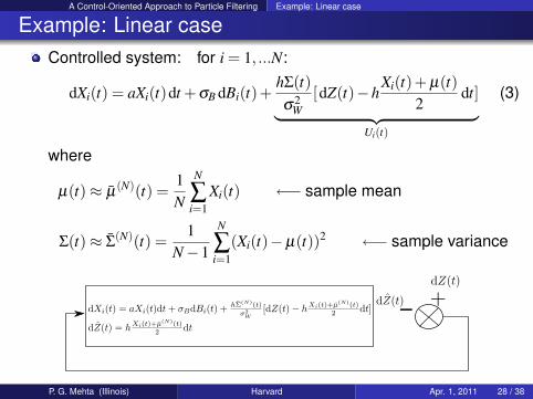
Example: Linear caseControlled system: for i = 1, ...N:
dXi(t) = aXi(t)dt +σB dBi(t)+hΣ(t)σ2
W[dZ(t)−h
Xi(t)+ µ(t)2
dt]︸ ︷︷ ︸Ui(t)
(3)
where
µ(t)≈ µ(N)(t) =
1N
N
∑i=1
Xi(t) ←− sample mean
Σ(t)≈ Σ(N)(t) =
1N−1
N
∑i=1
(Xi(t)−µ(t))2 ←− sample variance
P. G. Mehta (Illinois) Harvard Apr. 1, 2011 28 / 38
A Control-Oriented Approach to Particle Filtering Example: Linear case
Example: Linear case
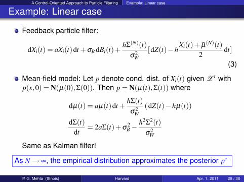
Feedback particle filter:
dXi(t) = aXi(t)dt +σB dBi(t)+hΣ(N)(t)
σ2W
[dZ(t)−hXi(t)+ µ(N)(t)
2dt]
(3)
Mean-field model: Let p denote cond. dist. of Xi(t) given Z t withp(x,0) = N(µ(0),Σ(0)). Then p = N(µ(t),Σ(t)) where
dµ(t) = aµ(t)dt +hΣ(t)σ2
W(dZ(t)−hµ(t))
dΣ(t)dt
= 2aΣ(t)+σ2B−
h2Σ2(t)σ2
W
Same as Kalman filter!
As N→ ∞, the empirical distribution approximates the posterior p∗
P. G. Mehta (Illinois) Harvard Apr. 1, 2011 29 / 38
A Control-Oriented Approach to Particle Filtering Example: Linear case
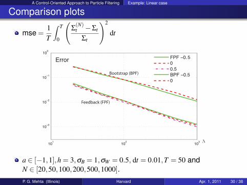
Comparison plots
mse =1T
∫ T
0
(Σ
(N)t −Σt
Σt
)2
dt
101
102
103
10−3
10−2
10−1
100
N
ErrorFPF −0.5
0
0.5
BPF −0.5
0
Bootstrap (BPF)
Feedback (FPF)
a ∈ [−1,1],h = 3,σB = 1,σW = 0.5, dt = 0.01,T = 50 andN ∈ [20,50,100,200,500,1000].P. G. Mehta (Illinois) Harvard Apr. 1, 2011 30 / 38
Methodology
Methodology: Variational problem
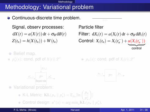
Continuous-discrete time problem. . . . . . . .
Signal, observ processes:dX(t) = a(X(t))dt +σB dB(t)Z(tn) = h(X(tn))+W (tn)
Particle filterFilter: dXi(t) = a(Xi(t)dt +σB dBi(t)Control: Xi(tn) = Xi(t−n )+u(Xi(t−n ))︸ ︷︷ ︸
control
Belief map.p∗n(x): cond. pdf of X(t)|Z t
Bayes rule
pn(x): cond. pdf of Xi(t)|Z t
Variational problem:
K-L Metric: KL(pn ‖ p∗n) = Epn [ln(
pn
p∗n
)]
Control design: u∗(x) = arg minuKL(pn ‖ p∗n).
P. G. Mehta (Illinois) Harvard Apr. 1, 2011 31 / 38
Methodology
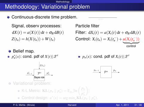
Methodology: Variational problem
Continuous-discrete time problem. . . . . . . .
Signal, observ processes:dX(t) = a(X(t))dt +σB dB(t)Z(tn) = h(X(tn))+W (tn)
Particle filterFilter: dXi(t) = a(Xi(t)dt +σB dBi(t)Control: Xi(tn) = Xi(t−n )+u(Xi(t−n ))︸ ︷︷ ︸
control
Belief map.p∗n(x): cond. pdf of X(t)|Z t
Bayes rule
pn(x): cond. pdf of Xi(t)|Z t
Variational problem:
K-L Metric: KL(pn ‖ p∗n) = Epn [ln(
pn
p∗n
)]
Control design: u∗(x) = arg minuKL(pn ‖ p∗n).
P. G. Mehta (Illinois) Harvard Apr. 1, 2011 31 / 38

Methodology
Methodology: Variational problem
Continuous-discrete time problem. . . . . . . .
Signal, observ processes:dX(t) = a(X(t))dt +σB dB(t)Z(tn) = h(X(tn))+W (tn)
Particle filterFilter: dXi(t) = a(Xi(t)dt +σB dBi(t)Control: Xi(tn) = Xi(t−n )+u(Xi(t−n ))︸ ︷︷ ︸
control
Belief map.p∗n(x): cond. pdf of X(t)|Z t
Bayes rule
pn(x): cond. pdf of Xi(t)|Z t
Variational problem:
K-L Metric: KL(pn ‖ p∗n) = Epn [ln(
pn
p∗n
)]
Control design: u∗(x) = arg minuKL(pn ‖ p∗n).
P. G. Mehta (Illinois) Harvard Apr. 1, 2011 31 / 38
Feedback particle filter
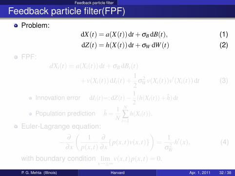
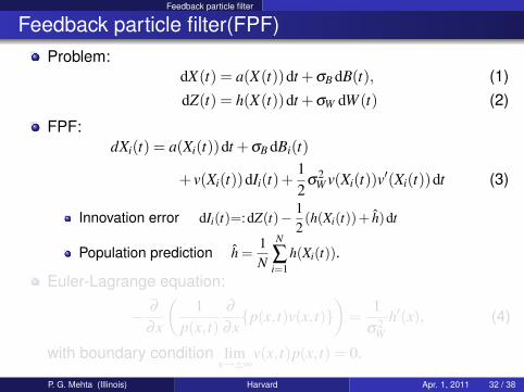
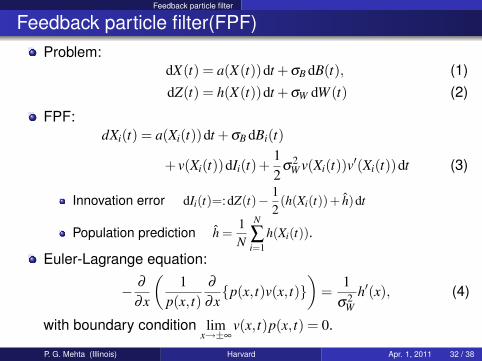
Feedback particle filter(FPF)Problem:
dX(t) = a(X(t))dt +σB dB(t), (1)dZ(t) = h(X(t))dt +σW dW (t) (2)
FPF:dXi(t) = a(Xi(t))dt +σB dBi(t)
+ v(Xi(t))dIi(t)+12
σ2W v(Xi(t))v′(Xi(t))dt (3)
Innovation error dIi(t)=:dZ(t)− 12(h(Xi(t))+ h)dt
Population prediction h =1N
N
∑i=1
h(Xi(t)).
Euler-Lagrange equation:
− ∂
∂x
(1
p(x, t)∂
∂xp(x, t)v(x, t)
)=
1σ2
Wh′(x), (4)
with boundary condition limx→±∞
v(x, t)p(x, t) = 0.
P. G. Mehta (Illinois) Harvard Apr. 1, 2011 32 / 38
Feedback particle filter
Feedback particle filter(FPF)Problem:
dX(t) = a(X(t))dt +σB dB(t), (1)dZ(t) = h(X(t))dt +σW dW (t) (2)
FPF:dXi(t) = a(Xi(t))dt +σB dBi(t)
+ v(Xi(t))dIi(t)+12
σ2W v(Xi(t))v′(Xi(t))dt (3)
Innovation error dIi(t)=:dZ(t)− 12(h(Xi(t))+ h)dt
Population prediction h =1N
N
∑i=1
h(Xi(t)).
Euler-Lagrange equation:
− ∂
∂x
(1
p(x, t)∂
∂xp(x, t)v(x, t)
)=
1σ2
Wh′(x), (4)
with boundary condition limx→±∞
v(x, t)p(x, t) = 0.
P. G. Mehta (Illinois) Harvard Apr. 1, 2011 32 / 38
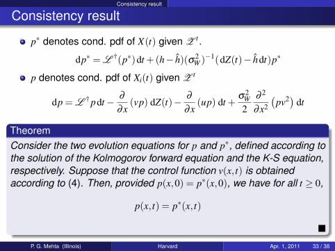
Consistency result
Consistency result
p∗ denotes cond. pdf of X(t) given Z t .
dp∗ = L †(p∗)dt +(h− h)(σ2W )−1(dZ(t)− hdt)p∗
p denotes cond. pdf of Xi(t) given Z t
dp = L † pdt− ∂
∂x(vp) dZ(t)− ∂
∂x(up) dt +
σ2W
2∂ 2
∂x2
(pv2) dt
TheoremConsider the two evolution equations for p and p∗, defined according tothe solution of the Kolmogorov forward equation and the K-S equation,respectively. Suppose that the control function v(x, t) is obtainedaccording to (4). Then, provided p(x,0) = p∗(x,0), we have for all t ≥ 0,
p(x, t) = p∗(x, t)
P. G. Mehta (Illinois) Harvard Apr. 1, 2011 33 / 38
Linear Gaussian case
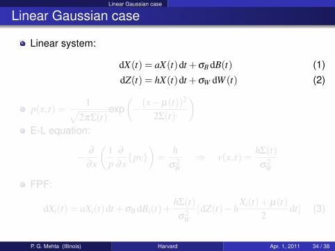
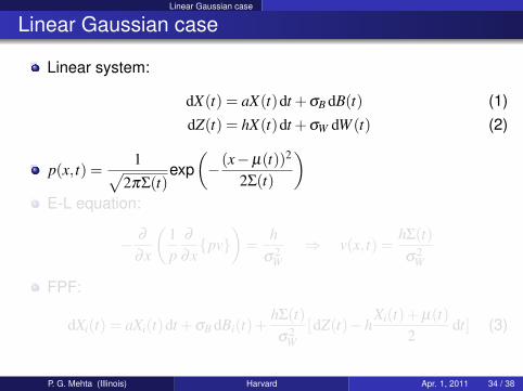
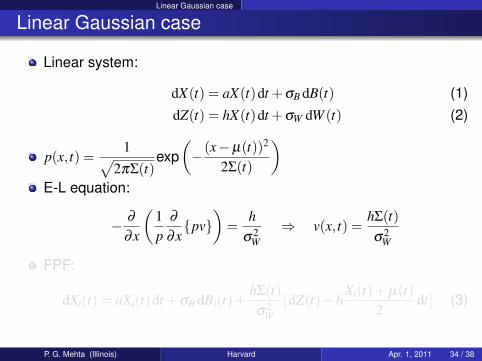
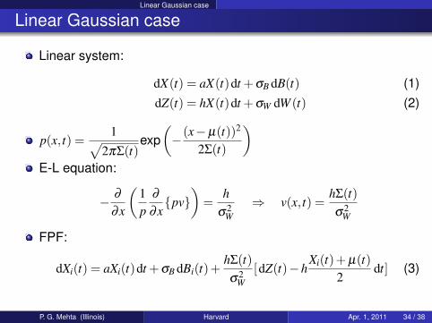
Linear Gaussian case
Linear system:
dX(t) = aX(t)dt +σB dB(t) (1)dZ(t) = hX(t)dt +σW dW (t) (2)
p(x, t) =1√
2πΣ(t)exp
(−(x−µ(t))2
2Σ(t)
)E-L equation:
− ∂
∂x
(1p
∂
∂xpv
)=
hσ2
W⇒ v(x, t) =
hΣ(t)σ2
W
FPF:
dXi(t) = aXi(t)dt +σB dBi(t)+hΣ(t)σ2
W[dZ(t)−h
Xi(t)+ µ(t)2
dt] (3)
P. G. Mehta (Illinois) Harvard Apr. 1, 2011 34 / 38
Linear Gaussian case
Linear Gaussian case
Linear system:
dX(t) = aX(t)dt +σB dB(t) (1)dZ(t) = hX(t)dt +σW dW (t) (2)
p(x, t) =1√
2πΣ(t)exp
(−(x−µ(t))2
2Σ(t)
)E-L equation:
− ∂
∂x
(1p
∂
∂xpv
)=
hσ2
W⇒ v(x, t) =
hΣ(t)σ2
W
FPF:
dXi(t) = aXi(t)dt +σB dBi(t)+hΣ(t)σ2
W[dZ(t)−h
Xi(t)+ µ(t)2
dt] (3)
P. G. Mehta (Illinois) Harvard Apr. 1, 2011 34 / 38
Example
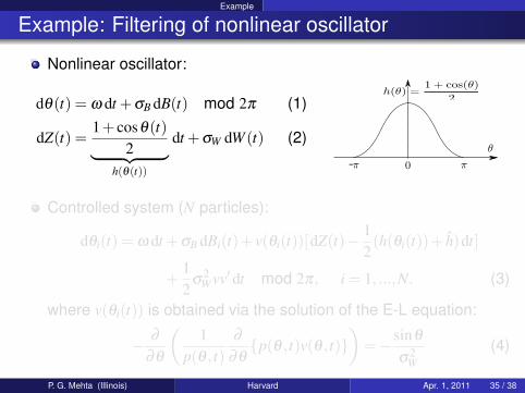
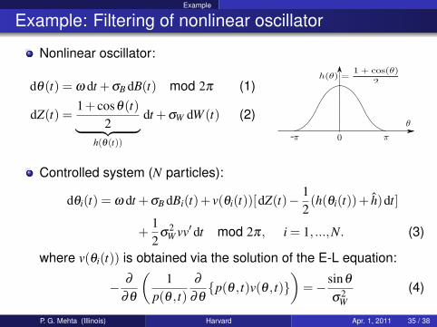
Example: Filtering of nonlinear oscillator
Nonlinear oscillator:
dθ(t) = ω dt +σB dB(t) mod 2π (1)
dZ(t) =1+ cosθ(t)
2︸ ︷︷ ︸h(θ(t))
dt +σW dW (t) (2)
-
Controlled system (N particles):
dθi(t) = ω dt +σB dBi(t)+ v(θi(t))[dZ(t)− 12(h(θi(t))+ h)dt]
+12
σ2W vv′ dt mod 2π, i = 1, ...,N. (3)
where v(θi(t)) is obtained via the solution of the E-L equation:
− ∂
∂θ
(1
p(θ , t)∂
∂θp(θ , t)v(θ , t)
)=−sinθ
σ2W
(4)
P. G. Mehta (Illinois) Harvard Apr. 1, 2011 35 / 38
Example
Example: Filtering of nonlinear oscillator
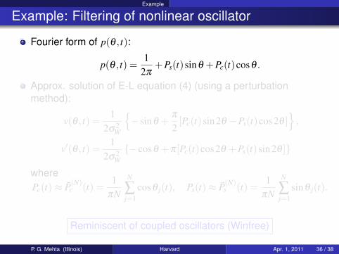
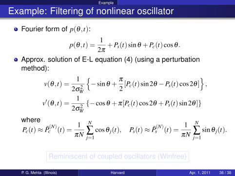
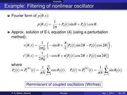
Fourier form of p(θ , t):
p(θ , t) =1
2π+Ps(t)sinθ +Pc(t)cosθ .
Approx. solution of E-L equation (4) (using a perturbationmethod):
v(θ , t) =1
2σ2W
−sinθ +
π
2[Pc(t)sin2θ −Ps(t)cos2θ ]
,
v′(θ , t) =1
2σ2W−cosθ +π[Pc(t)cos2θ +Ps(t)sin2θ ]
wherePc(t)≈ P(N)
c (t) =1
πN
N
∑j=1
cosθ j(t), Ps(t)≈ P(N)s (t) =
1πN
N
∑j=1
sinθ j(t).
Reminiscent of coupled oscillators (Winfree)
P. G. Mehta (Illinois) Harvard Apr. 1, 2011 36 / 38
Example
Example: Filtering of nonlinear oscillator
Fourier form of p(θ , t):
p(θ , t) =1
2π+Ps(t)sinθ +Pc(t)cosθ .
Approx. solution of E-L equation (4) (using a perturbationmethod):
v(θ , t) =1
2σ2W
−sinθ +
π
2[Pc(t)sin2θ −Ps(t)cos2θ ]
,
v′(θ , t) =1
2σ2W−cosθ +π[Pc(t)cos2θ +Ps(t)sin2θ ]
wherePc(t)≈ P(N)
c (t) =1
πN
N
∑j=1
cosθ j(t), Ps(t)≈ P(N)s (t) =
1πN
N
∑j=1
sinθ j(t).
Reminiscent of coupled oscillators (Winfree)
P. G. Mehta (Illinois) Harvard Apr. 1, 2011 36 / 38
Example
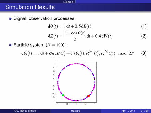
Simulation Results
Signal, observation processes:
dθ(t) = 1dt +0.5dB(t) (1)
dZ(t) =1+ cosθ(t)
2dt +0.4dW (t) (2)
Particle system (N = 100):
dθi(t) = 1dt +σB dBi(t)+U(θi(t); P(N)c (t), P(N)
s (t)) mod 2π (3)
P. G. Mehta (Illinois) Harvard Apr. 1, 2011 37 / 38
Example
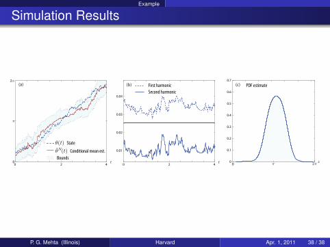
Simulation Results
0 2 4 0 2 4
0.01
0.02
0.03
0.04
00
0.1
0.2
0.3
0.4
0.5
0.6
0.7
t t xπ 2π0
π
2π(a) (b) (c)First harmonic PDF estimate
Second harmonic
Bounds
State
Conditional mean est.
θ(t)θN(t)
P. G. Mehta (Illinois) Harvard Apr. 1, 2011 38 / 38

Thank you!
Website: http://www.mechse.illinois.edu/research/mehtapg
Collaborators
Huibing Yin Tao Yang Sean Meyn Uday Shanbhag
“Synchronization of coupled oscillators is a game,” IEEE TAC, ACC 2010“Learning in Mean-Field Oscillator Games,” CDC 2010“On the Efficiency of Equilibria in Mean-field Oscillator Games,” ACC 2011“A Control-oriented Approach for Particle Filtering,” ACC2011, CDC2011
Part III
Learning in mean-field game
Learning Q-function approximation
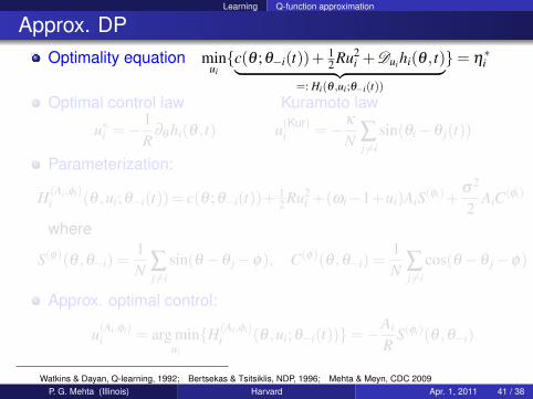
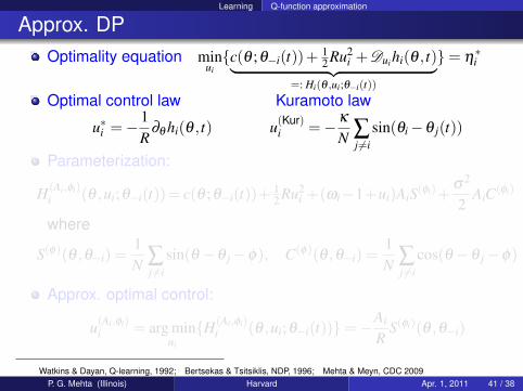
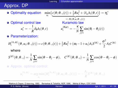
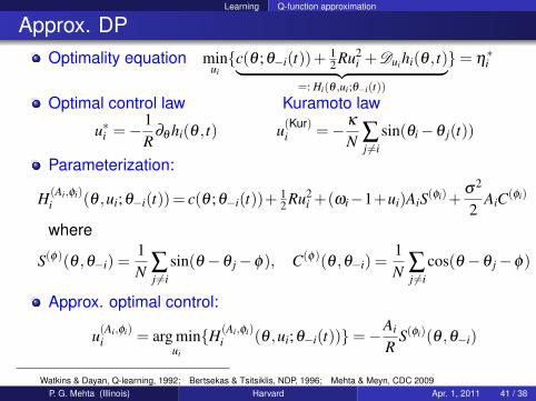
Approx. DPOptimality equation min
uic(θ ;θ−i(t))+ 1
2 Ru2i +Duihi(θ , t)︸ ︷︷ ︸
=: Hi(θ ,ui;θ−i(t))
= η∗i
Optimal control law Kuramoto law
u∗i =− 1R
∂θ hi(θ , t) u(Kur)i =−κ
N ∑j 6=i
sin(θi−θ j(t))
Parameterization:
H(Ai,φi)i (θ ,ui;θ−i(t))= c(θ ;θ−i(t))+ 1
2 Ru2i +(ωi−1+ui)AiS(φi)+
σ2
2AiC(φi)
where
S(φ)(θ ,θ−i) =1N ∑
j 6=isin(θ −θ j−φ), C(φ)(θ ,θ−i) =
1N ∑
j 6=icos(θ −θ j−φ)
Approx. optimal control:
u(Ai,φi)i = arg min
ui
H(Ai,φi)i (θ ,ui;θ−i(t))=−Ai
RS(φi)(θ ,θ−i)
Watkins & Dayan, Q-learning, 1992; Bertsekas & Tsitsiklis, NDP, 1996; Mehta & Meyn, CDC 2009P. G. Mehta (Illinois) Harvard Apr. 1, 2011 41 / 38
Learning Q-function approximation
Approx. DPOptimality equation min
uic(θ ;θ−i(t))+ 1
2 Ru2i +Duihi(θ , t)︸ ︷︷ ︸
=: Hi(θ ,ui;θ−i(t))
= η∗i
Optimal control law Kuramoto law
u∗i =− 1R
∂θ hi(θ , t) u(Kur)i =−κ
N ∑j 6=i
sin(θi−θ j(t))
Parameterization:
H(Ai,φi)i (θ ,ui;θ−i(t))= c(θ ;θ−i(t))+ 1
2 Ru2i +(ωi−1+ui)AiS(φi)+
σ2
2AiC(φi)
where
S(φ)(θ ,θ−i) =1N ∑
j 6=isin(θ −θ j−φ), C(φ)(θ ,θ−i) =
1N ∑
j 6=icos(θ −θ j−φ)
Approx. optimal control:
u(Ai,φi)i = arg min
ui
H(Ai,φi)i (θ ,ui;θ−i(t))=−Ai
RS(φi)(θ ,θ−i)
Watkins & Dayan, Q-learning, 1992; Bertsekas & Tsitsiklis, NDP, 1996; Mehta & Meyn, CDC 2009P. G. Mehta (Illinois) Harvard Apr. 1, 2011 41 / 38
Learning Stochastic approx.
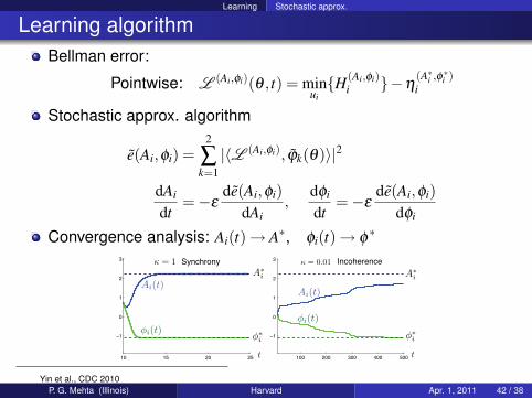
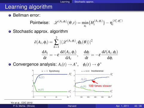
Learning algorithmBellman error:
Pointwise: L (Ai,φi)(θ , t) = minuiH(Ai,φi)
i −η(A∗i ,φ
∗i )
i
Stochastic approx. algorithm
e(Ai,φi) =2
∑k=1|〈L (Ai,φi), ϕk(θ)〉|2
dAi
dt=−ε
de(Ai,φi)dAi
,dφi
dt=−ε
de(Ai,φi)dφi
Convergence analysis: Ai(t)→ A∗, φi(t)→ φ∗
100 200 300 400 500
−1
0
1
2
3
10 15 20 25
−1
0
1
2
3 Synchrony Incoherence
Yin et al., CDC 2010P. G. Mehta (Illinois) Harvard Apr. 1, 2011 42 / 38
Learning Stochastic approx.
Learning algorithmBellman error:
Pointwise: L (Ai,φi)(θ , t) = minuiH(Ai,φi)
i −η(A∗i ,φ
∗i )
i
Stochastic approx. algorithm
e(Ai,φi) =2
∑k=1|〈L (Ai,φi), ϕk(θ)〉|2
dAi
dt=−ε
de(Ai,φi)dAi
,dφi
dt=−ε
de(Ai,φi)dφi
Convergence analysis: Ai(t)→ A∗, φi(t)→ φ∗
100 200 300 400 500
−1
0
1
2
3
10 15 20 25
−1
0
1
2
3 Synchrony Incoherence
Yin et al., CDC 2010P. G. Mehta (Illinois) Harvard Apr. 1, 2011 42 / 38
Learning Bifurcation diagram
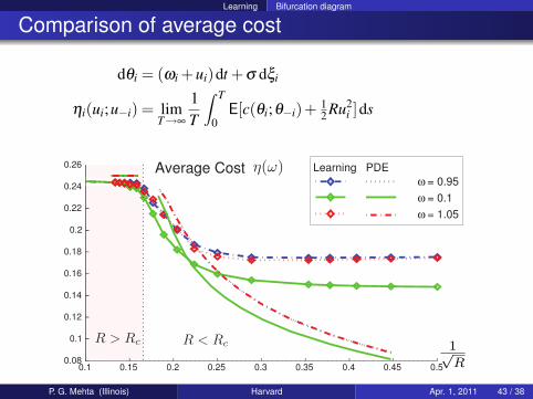
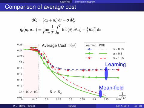
Comparison of average cost
dθi = (ωi +ui)dt +σ dξi
ηi(ui;u−i) = limT→∞
1T
∫ T
0E[c(θi;θ−i)+ 1
2 Ru2i ]ds
P. G. Mehta (Illinois) Harvard Apr. 1, 2011 43 / 38
Learning Bifurcation diagram
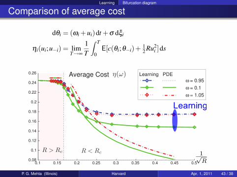
Comparison of average cost
dθi = (ωi +ui)dt +σ dξi
ηi(ui;u−i) = limT→∞
1T
∫ T
0E[c(θi;θ−i)+ 1
2 Ru2i ]ds
Learning
P. G. Mehta (Illinois) Harvard Apr. 1, 2011 43 / 38
Learning Bifurcation diagram
Comparison of average cost
dθi = (ωi +ui)dt +σ dξi
ηi(ui;u−i) = limT→∞
1T
∫ T
0E[c(θi;θ−i)+ 1
2 Ru2i ]ds
Learning
Mean-field
P. G. Mehta (Illinois) Harvard Apr. 1, 2011 43 / 38
Part IV
Apendix
Analysis of phase transition Incoherence solution
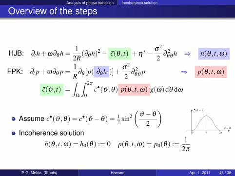
Overview of the steps
HJB: ∂th+ω∂θ h =1
2R(∂θ h)2− c(θ , t) +η
∗− σ2
2∂
2θθ h ⇒ h(θ , t,ω)
FPK: ∂t p+ω∂θ p =1R
∂θ [p( ∂θ h )]+σ2
2∂
2θθ p ⇒ p(θ , t,ω)
c(ϑ , t) =∫
Ω
∫ 2π
0c•(ϑ ,θ) p(θ , t,ω) g(ω)dθ dω
Assume c•(ϑ ,θ) = c•(ϑ −θ) = 12 sin2
(ϑ −θ
2
)Incoherence solution
h(θ , t,ω) = h0(θ) := 0 p(θ , t,ω) = p0(θ) :=1
2π
P. G. Mehta (Illinois) Harvard Apr. 1, 2011 45 / 38
Analysis of phase transition Bifurcation analysis
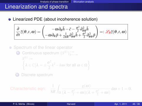
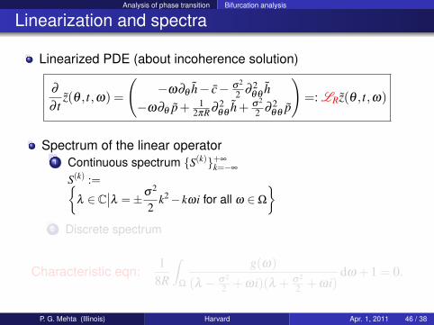
Linearization and spectra
Linearized PDE (about incoherence solution)
∂
∂ tz(θ , t,ω) =
(−ω∂θ h− c− σ2
2 ∂ 2θθ
h−ω∂θ p+ 1
2πR ∂ 2θθ
h+ σ2
2 ∂ 2θθ
p
)=: LRz(θ , t,ω)
Spectrum of the linear operator1 Continuous spectrum S(k)+∞
k=−∞
S(k) :=λ ∈ C
∣∣λ =±σ2
2k2− kωi for all ω ∈Ω
2 Discrete spectrum
Characteristic eqn:1
8R
∫Ω
g(ω)
(λ − σ2
2 +ωi)(λ + σ2
2 +ωi)dω +1 = 0.
P. G. Mehta (Illinois) Harvard Apr. 1, 2011 46 / 38
Analysis of phase transition Bifurcation analysis
Linearization and spectra
Linearized PDE (about incoherence solution)
∂
∂ tz(θ , t,ω) =
(−ω∂θ h− c− σ2
2 ∂ 2θθ
h−ω∂θ p+ 1
2πR ∂ 2θθ
h+ σ2
2 ∂ 2θθ
p
)=: LRz(θ , t,ω)
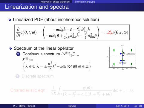
Spectrum of the linear operator1 Continuous spectrum S(k)+∞
k=−∞
S(k) :=λ ∈ C
∣∣λ =±σ2
2k2− kωi for all ω ∈Ω
−0.2 −0.1 0 0.1 0.2 0.3
−3
−2
−1
0
1
2
3
real
ima
g
γ = 0.1
R decreases
k=2 k=2
k=1 k=1
2 Discrete spectrum
Characteristic eqn:1
8R
∫Ω
g(ω)
(λ − σ2
2 +ωi)(λ + σ2
2 +ωi)dω +1 = 0.
P. G. Mehta (Illinois) Harvard Apr. 1, 2011 46 / 38
Analysis of phase transition Bifurcation analysis
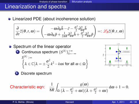
Linearization and spectra
Linearized PDE (about incoherence solution)
∂
∂ tz(θ , t,ω) =
(−ω∂θ h− c− σ2
2 ∂ 2θθ
h−ω∂θ p+ 1
2πR ∂ 2θθ
h+ σ2
2 ∂ 2θθ
p
)=: LRz(θ , t,ω)
Spectrum of the linear operator1 Continuous spectrum S(k)+∞
k=−∞
S(k) :=λ ∈ C
∣∣λ =±σ2
2k2− kωi for all ω ∈Ω
−0.2 −0.1 0 0.1 0.2 0.3
−3
−2
−1
0
1
2
3
real
ima
g
γ = 0.1
R decreases
k=2 k=2
k=1 k=1
2 Discrete spectrum
Characteristic eqn:1
8R
∫Ω
g(ω)
(λ − σ2
2 +ωi)(λ + σ2
2 +ωi)dω +1 = 0.
P. G. Mehta (Illinois) Harvard Apr. 1, 2011 46 / 38
Analysis of phase transition Bifurcation analysis
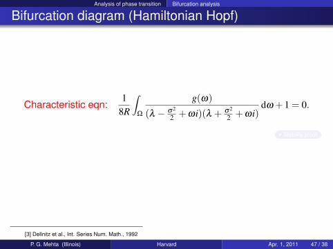
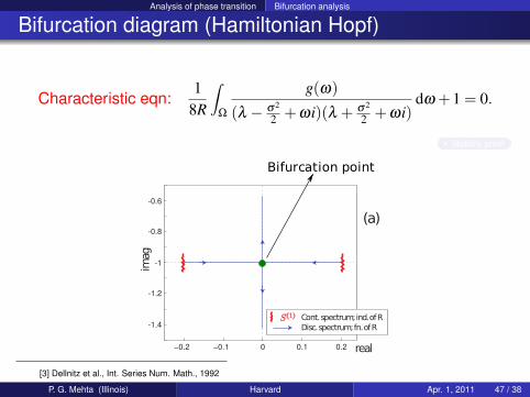
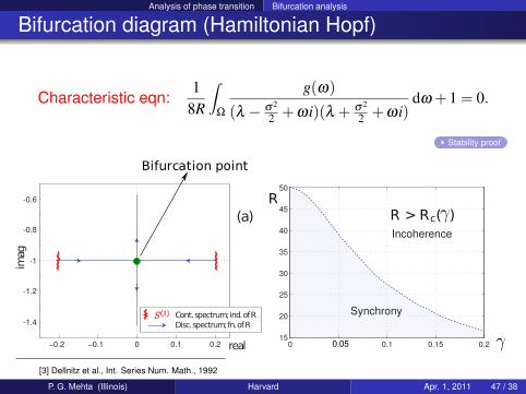
Bifurcation diagram (Hamiltonian Hopf)
Characteristic eqn:1
8R
∫Ω
g(ω)
(λ − σ2
2 +ωi)(λ + σ2
2 +ωi)dω +1 = 0.
Stability proof
[3] Dellnitz et al., Int. Series Num. Math., 1992
P. G. Mehta (Illinois) Harvard Apr. 1, 2011 47 / 38
Analysis of phase transition Bifurcation analysis
Bifurcation diagram (Hamiltonian Hopf)
Characteristic eqn:1
8R
∫Ω
g(ω)
(λ − σ2
2 +ωi)(λ + σ2
2 +ωi)dω +1 = 0.
Stability proof
−0.2 −0.1 0 0.1 0.2
-0.6
-0.8
-1
-1.2
-1.4
real
imag
(a)
Cont. spectrum; ind. of RDisc. spectrum; fn. of R
Bifurcation point
0 0.05 0.1 0.15 0.215
20
25
30
35
40
45
50
Incoherence
R > RR
c(γ
γ
) (c))
Synchrony
0.05
[3] Dellnitz et al., Int. Series Num. Math., 1992
P. G. Mehta (Illinois) Harvard Apr. 1, 2011 47 / 38
Analysis of phase transition Numerics
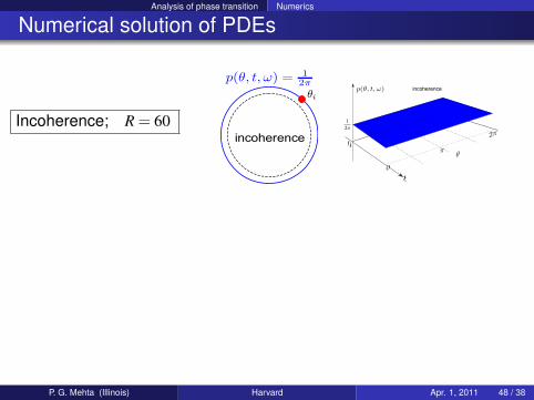
Numerical solution of PDEs
Incoherence; R = 60
incoherence
P. G. Mehta (Illinois) Harvard Apr. 1, 2011 48 / 38
Analysis of phase transition Numerics
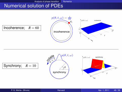
Numerical solution of PDEs
Incoherence; R = 60
incoherence
Synchrony; R = 10
synchrony
synchrony
P. G. Mehta (Illinois) Harvard Apr. 1, 2011 48 / 38
Analysis of phase transition Numerics
Bifurcation diagram
Locking
0 0.1 0.2
0.15
0.2
0.25
R−1/ 2
γγIncoherence
R > Rc(γ)
Synchrony
Incoherence R−1/2
η(ω)
0. 1 0.15 0. 2 0.25 0. 3 0.35
0. 1
0.15
0. 2
0.25
ω = 0.95
ω = 1
ω = 1.05
R > Rc
η(ω) = η0
R < Rc
η(ω) < η0
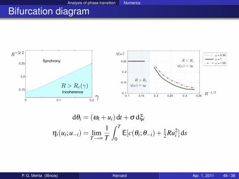
dθi = (ωi +ui)dt +σ dξi
ηi(ui;u−i) = limT→∞
1T
∫ T
0E[c(θi;θ−i)+ 1
2 Ru2i ]ds
P. G. Mehta (Illinois) Harvard Apr. 1, 2011 49 / 38
Analysis of phase transition Numerics
Bifurcation diagram
Locking
0 0.1 0.2
0.15
0.2
0.25
R−1/ 2
γγIncoherence
R > Rc(γ)
Synchrony
Incoherence R−1/2
η(ω)
0. 1 0.15 0. 2 0.25 0. 3 0.35
0. 1
0.15
0. 2
0.25
ω = 0.95
ω = 1
ω = 1.05
R > Rc
η(ω) = η0
R < Rc
η(ω) < η0
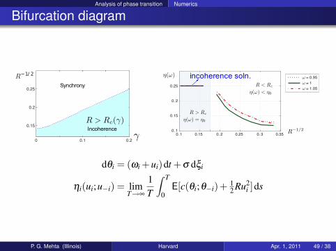
incoherence soln.
dθi = (ωi +ui)dt +σ dξi
ηi(ui;u−i) = limT→∞
1T
∫ T
0E[c(θi;θ−i)+ 1
2 Ru2i ]ds
P. G. Mehta (Illinois) Harvard Apr. 1, 2011 49 / 38
Analysis of phase transition Numerics
Bifurcation diagram
Locking
0 0.1 0.2
0.15
0.2
0.25
R−1/ 2
γγIncoherence
R > Rc(γ)
Synchrony
Incoherence R−1/2
η(ω)
0. 1 0.15 0. 2 0.25 0. 3 0.35
0. 1
0.15
0. 2
0.25
ω = 0.95
ω = 1
ω = 1.05
R > Rc
η(ω) = η0
R < Rc
η(ω) < η0
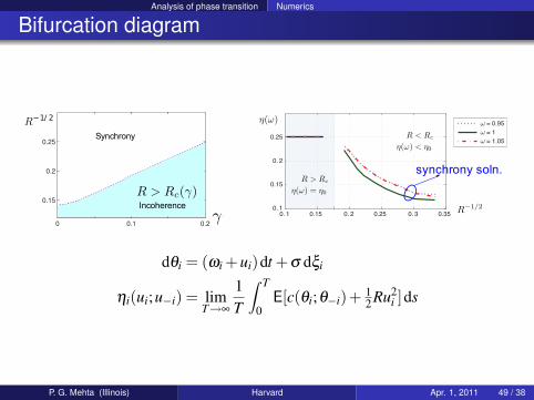
synchrony soln.
dθi = (ωi +ui)dt +σ dξi
ηi(ui;u−i) = limT→∞
1T
∫ T
0E[c(θi;θ−i)+ 1
2 Ru2i ]ds
P. G. Mehta (Illinois) Harvard Apr. 1, 2011 49 / 38
Analysis of phase transition Numerics
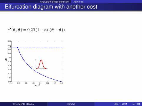
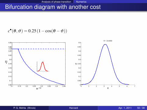
Bifurcation diagram with another cost
c•(θ ,ϑ) = 0.25(1− cos(θ −ϑ))
0.1 0.15 0.2 0.25 0.3 0.35 0.4 0.450.08
0.1
0.12
0.14
0.16
0.18
0.2
0.22
0.24
0.26
0.28
R−1/2
0 1 2 3 4 5 6 70
0.05
0.1
0.15
0.2
0.25
0.3
0.35
0.4
0.45
0.5
θ
p
R = 23.8359
P. G. Mehta (Illinois) Harvard Apr. 1, 2011 50 / 38
Analysis of phase transition Numerics
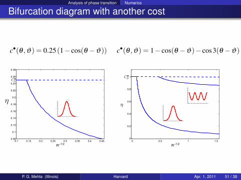
Bifurcation diagram with another cost
c•(θ ,ϑ) = 0.25(1− cos(θ −ϑ))
0.1 0.15 0.2 0.25 0.3 0.35 0.4 0.450.08
0.1
0.12
0.14
0.16
0.18
0.2
0.22
0.24
0.26
0.28
R−1/2
0 1 2 3 4 5 6 70
0.05
0.1
0.15
0.2
0.25
0.3
0.35
0.4
0.45
0.5
θ
p
R = 23.8359
0 1 2 3 4 5 6 70
0.05
0.1
0.15
0.2
0.25
0.3
0.35
0.4
0.45
0.5
θ
p
R = 23.8359
P. G. Mehta (Illinois) Harvard Apr. 1, 2011 50 / 38
Analysis of phase transition Numerics
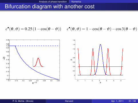
Bifurcation diagram with another cost
c•(θ ,ϑ) = 0.25(1− cos(θ −ϑ))
0.1 0.15 0.2 0.25 0.3 0.35 0.4 0.450.08
0.1
0.12
0.14
0.16
0.18
0.2
0.22
0.24
0.26
0.28
R−1/2
0 1 2 3 4 5 6 70
0.05
0.1
0.15
0.2
0.25
0.3
0.35
0.4
0.45
0.5
θ
p
R = 23.8359
c•(θ ,ϑ) = 1− cos(θ −ϑ)− cos3(θ −ϑ)
0 0.5 1 1.50
0.2
0.4
0.6
0.8
1
R−1/2
0 1 2 3 4 5 60
0.1
0.2
0.3
0.4
0.5
0.6
0.7
0.8
0 1 2 3 4 5 60
0.1
0.2
0.3
0.4
0.5
0.6
0.7
0.8
P. G. Mehta (Illinois) Harvard Apr. 1, 2011 51 / 38
Analysis of phase transition Numerics
Bifurcation diagram with another cost
c•(θ ,ϑ) = 0.25(1− cos(θ −ϑ))
0.1 0.15 0.2 0.25 0.3 0.35 0.4 0.450.08
0.1
0.12
0.14
0.16
0.18
0.2
0.22
0.24
0.26
0.28
R−1/2
0 1 2 3 4 5 6 70
0.05
0.1
0.15
0.2
0.25
0.3
0.35
0.4
0.45
0.5
θ
p
R = 23.8359
c•(θ ,ϑ) = 1− cos(θ −ϑ)− cos3(θ −ϑ)
0 1 2 3 4 5 6
0
0.2
0.4
0.6
0.8
1
1.2
1.4
1.6
θ
p
P. G. Mehta (Illinois) Harvard Apr. 1, 2011 51 / 38
Feedback particle filter
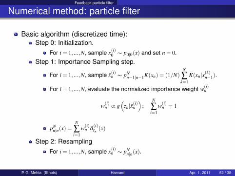
Numerical method: particle filter
Basic algorithm (discretized time):Step 0: Initialization.
For i = 1, ...,N, sample x(i)0 ∼ p0|0(x) and set n = 0.
Step 1: Importance Sampling step.
For i = 1, ...,N, sample x(i)n ∼ pN
n−1|n−1K(xn) = (1/N)N
∑k=1
K(xn|x(k)n−1).
For i = 1, ...,N, evaluate the normalized importance weight w(i)n
w(i)n ∝ g
(zn|x
(i)n
);
N
∑i=1
w(i)n = 1
pNn|n(x) =
N
∑i=1
w(i)n δ
(i)xn
(x)
Step 2: ResamplingFor i = 1, ...,N, sample x(i)
n ∼ pNn|n(x).
P. G. Mehta (Illinois) Harvard Apr. 1, 2011 52 / 38
Feedback particle filter
Calculation of KL divergence
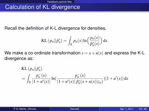
Recall the definition of K-L divergence for densities,
KL(pn‖ p∗n) =∫
Rpn(s) ln
( pn(s)p∗n(s)
)ds.
We make a co-ordinate transformation s = x+u(x) and express the K-Ldivergence as:
KL(pn‖ p∗n)
=∫
R
p−n (x)|1+u′(x)|
ln(p−n (x)
|1+u′(x)| p∗n(x+u(x)|zn))|1+u′(x)|dx
P. G. Mehta (Illinois) Harvard Apr. 1, 2011 53 / 38
Feedback particle filter
Derivation of Euler-Lagrange equation
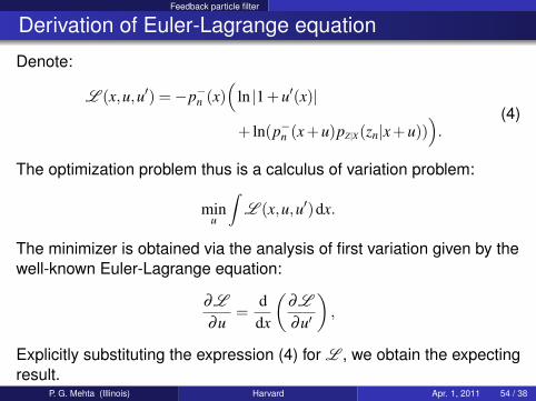
Denote:
L (x,u,u′) =−p−n (x)(
ln |1+u′(x)|
+ ln(p−n (x+u)pZ|X(zn|x+u))).
(4)
The optimization problem thus is a calculus of variation problem:
minu
∫L (x,u,u′)dx.
The minimizer is obtained via the analysis of first variation given by thewell-known Euler-Lagrange equation:
∂L
∂u=
ddx
(∂L
∂u′
),
Explicitly substituting the expression (4) for L , we obtain the expectingresult.
P. G. Mehta (Illinois) Harvard Apr. 1, 2011 54 / 38
Feedback particle filter
Simulation Results
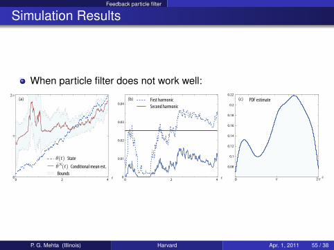
When particle filter does not work well:
Bounds
0
0.08
0.1
0.12
0.14
0.16
0.18
0.2
0.22
t t
First harmonic PDF estimate
Second harmonic
xπ 2π0
π
2π
0 2 4 0 2 40
0.01
0.02
0.03
0.04
(a) (b) (c)
State
Conditional mean est.
θ(t)θN(t)
P. G. Mehta (Illinois) Harvard Apr. 1, 2011 55 / 38
Feedback particle filter
Derivation of FPK for FPF
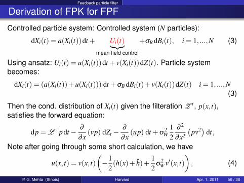
Controlled particle system: Controlled system (N particles):
dXi(t) = a(Xi(t))dt + Ui(t)︸︷︷︸mean field control
+σB dBi(t), i = 1, ...,N (3)
Using ansatz: Ui(t) = u(Xi(t))dt + v(Xi(t))dZ(t). Particle systembecomes:
dXi(t) = (a(Xi(t))+u(Xi(t))) dt +σB dBi(t)+ v(Xi(t))dZ(t) i = 1, ...,N(3)
Then the cond. distribution of Xi(t) given the filteration Z t , p(x, t),satisfies the forward equation:
dp = L † pdt− ∂
∂x(vp) dZt −
∂
∂x(up) dt +σ
2W
12
∂ 2
∂x2
(pv2) dt,
Note after going through some short calculation, we have
u(x, t) = v(x, t)(−1
2(h(x)+ h)+
12
σ2W v′(x, t)
), (4)
P. G. Mehta (Illinois) Harvard Apr. 1, 2011 56 / 38
Feedback particle filter
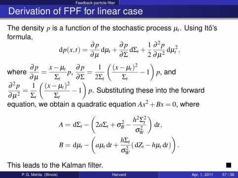
Derivation of FPF for linear case
The density p is a function of the stochastic process µt . Using Itô’sformula,
dp(x, t) =∂ p∂ µ
dµt +∂ p∂Σ
dΣt +12
∂ 2 p∂ µ2 dµ
2t ,
where∂ p∂ µ
=x−µt
Σtp,
∂ p∂Σ
=1
2Σt
((x−µt)2
Σt−1)
p, and
∂ 2 p∂ µ2 =
1Σt
((x−µt)2
Σt−1)
p. Substituting these into the forward
equation, we obtain a quadratic equation Ax2 +Bx = 0, where
A = dΣt −(
2aΣt +σ2B−
h2Σ2t
σ2W
)dt,
B = dµt −(
aµt dt +hΣt
σ2W
(dZt −hµt dt))
.
This leads to the Kalman filter.P. G. Mehta (Illinois) Harvard Apr. 1, 2011 57 / 38
Feedback particle filter
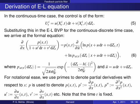
Derivation of E-L equation
In the continuous-time case, the control is of the form:
U it = u(X i
t , t)dt + v(X it , t)dZt . (5)
Substituting this in the E-L BVP for the continuous-discrete time case,we arrive at the formal equation:
∂
∂x
(p(x, t)
1+u′ dt + v′ dZt
)=p(x, t)
∂
∂ u
(ln p(x+udt + vdZt , t)
+ ln pdZ|X(dZt | x+udt + vdZt)), (6)
where pdZ|X(dZt |·) =1√
2πσ2W
exp(−(dZt −h(·))2
2σ2W
)and u = udt + vdZt .
For notational ease, we use primes to denote partial derivatives with
respect to x: p is used to denote p(x, t), p′ :=∂ p∂x
(x, t), p′′ :=∂ 2 p∂x2 (x, t),
u′ :=∂u∂x
(x, t), v′ :=∂v∂x
(x, t) etc. Note that the time t is fixed.
P. G. Mehta (Illinois) Harvard Apr. 1, 2011 58 / 38
Feedback particle filter
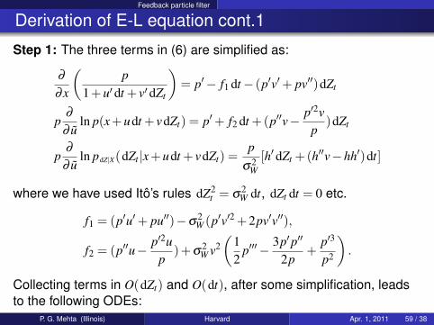
Derivation of E-L equation cont.1
Step 1: The three terms in (6) are simplified as:
∂
∂x
(p
1+u′ dt + v′ dZt
)= p′− f1 dt− (p′v′+ pv′′)dZt
p∂
∂ uln p(x+udt + vdZt) = p′+ f2 dt +(p′′v− p′2v
p)dZt
p∂
∂ uln pdZ|X(dZt |x+udt + vdZt) =
pσ2
W[h′ dZt +(h′′v−hh′)dt]
where we have used Itô’s rules dZ2t = σ
2W dt, dZt dt = 0 etc.
f1 = (p′u′+ pu′′)−σ2W (p′v′2 +2pv′v′′),
f2 = (p′′u− p′2up
)+σ2W v2
(12
p′′′− 3p′p′′
2p+
p′3
p2
).
Collecting terms in O(dZt) and O(dt), after some simplification, leadsto the following ODEs:
P. G. Mehta (Illinois) Harvard Apr. 1, 2011 59 / 38
Feedback particle filter
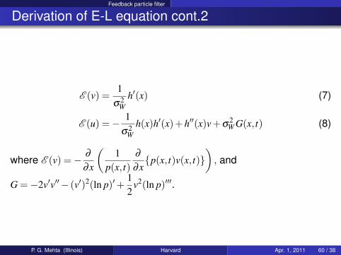
Derivation of E-L equation cont.2
E (v) =1
σ2W
h′(x) (7)
E (u) =− 1σ2
Wh(x)h′(x)+h′′(x)v+σ
2W G(x, t) (8)
where E (v) =− ∂
∂x
(1
p(x, t)∂
∂xp(x, t)v(x, t)
), and
G =−2v′v′′− (v′)2(ln p)′+12
v2(ln p)′′′.
P. G. Mehta (Illinois) Harvard Apr. 1, 2011 60 / 38
Feedback particle filter
Derivation of E-L equation cont.3
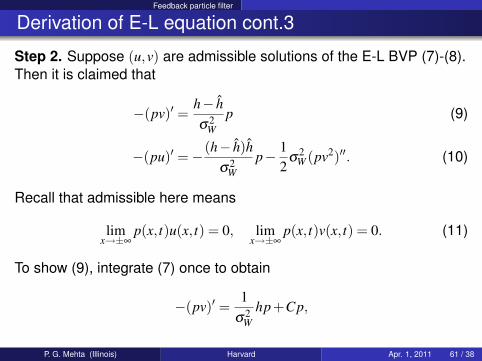
Step 2. Suppose (u,v) are admissible solutions of the E-L BVP (7)-(8).Then it is claimed that
−(pv)′ =h− hσ2
Wp (9)
−(pu)′ =−(h− h)hσ2
Wp− 1
2σ
2W (pv2)′′. (10)
Recall that admissible here means
limx→±∞
p(x, t)u(x, t) = 0, limx→±∞
p(x, t)v(x, t) = 0. (11)
To show (9), integrate (7) once to obtain
−(pv)′ =1
σ2W
hp+Cp,
P. G. Mehta (Illinois) Harvard Apr. 1, 2011 61 / 38

Feedback particle filter
Derivation of E-L equation cont.4
where the constant of integration C =− hσ2
Wis obtained by integrating
once again between −∞ to ∞ and using the boundary conditions forv (11). This gives (9). To show (10), we denote its right hand side as Rand claim (
R
p
)′=−hh′
σ2W
+h′′v+σ2W G. (12)
The equation (10) then follows by using the ODE (8) together with theboundary conditions for u (11). The verification of the claim involves astraightforward calculation, where we use (7) to obtain expressions forh′ and v′′. The details of this calculation are omitted on account ofspace.
P. G. Mehta (Illinois) Harvard Apr. 1, 2011 62 / 38
Feedback particle filter
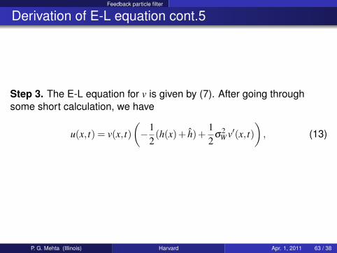
Derivation of E-L equation cont.5
Step 3. The E-L equation for v is given by (7). After going throughsome short calculation, we have
u(x, t) = v(x, t)(−1
2(h(x)+ h)+
12
σ2W v′(x, t)
), (13)
P. G. Mehta (Illinois) Harvard Apr. 1, 2011 63 / 38
Bibliography
Dimitri P. Bertsekas.Dynamic Programming and Optimal Control, volume 1.Athena Scientific, Belmont, Massachusetts, 1995.
Eric Brown, Jeff Moehlis, and Philip Holmes.On the phase reduction and response dynamics of neuraloscillator populations.Neural Computation, 16(4):673–715, 2004.
M. Dellnitz, J.E. Marsden, I. Melbourne, and J. Scheurle.Generic bifurcations of pendula.Int. Series Num. Math., 104:111–122, 1992.
A. Doucet, N. de Freitas, and N. Gordon.Sequential Monte-Carlo Methods in Practice.Springer-Verlag, April 2001.
N. J. Gordon, D. J. Salmond, and A. F. M. Smith.Novel approach to nonlinear/non-Gaussian Bayesian stateestimation.P. G. Mehta (Illinois) Harvard Apr. 1, 2011 63 / 38
Bibliography
IEE Proceedings F Radar and Signal Processing, 140(2):107–113,1993.
J. Guckenheimer.Isochrons and phaseless sets.J. Math. Biol., 1:259–273, 1975.
M. Huang, P. E. Caines, and R. P. Malhame.Large-population cost-coupled LQG problems with nonuniformagents: Individual-mass behavior and decentralized ε-Nashequilibria.52(9):1560–1571, 2007.
Minyi Huang, Peter E. Caines, and Roland P. Malhame.Large-population cost-coupled LQG problems with nonuniformagents: Individual-mass behavior and decentralized ε-nashequilibria.IEEE transactions on automatic control, 52(9):1560–1571, 2007.
R. E. Kalman.
P. G. Mehta (Illinois) Harvard Apr. 1, 2011 63 / 38

Bibliography
A new approach to linear filtering and prediction problems.Journal of Basic Engineering, 82(1):35–45, 1960.
Y. Kuramoto.International Symposium on Mathematical Problems in TheoreticalPhysics, volume 39 of Lecture Notes in Physics.Springer-Verlag, 1975.
H. J. Kushner.On the differential equations satisfied by conditional probabilitydensities of markov process.SIAM J. Control, 2:106–119, 1964.
J. Lasry and P. Lions.Mean field games.Japanese Journal of Mathematics, 2(2):229–260, 2007.
Jean-Michel Lasry and Pierre-Louis Lions.Mean field games.Japan. J. Math., 2:229–260, 2007.
P. G. Mehta (Illinois) Harvard Apr. 1, 2011 63 / 38
Bibliography
Sean P. Meyn.The policy iteration algorithm for average reward markov decisionprocesses with general state space.IEEE Transactions on Automatic Control, 42(12):1663–1680,December 1997.
S. H. Strogatz and R. E. Mirollo.Stability of incoherence in a population of coupled oscillators.Journal of Statistical Physics, 63:613–635, May 1991.
G. Y. Weintraub, L. Benkard, and B. Van Roy.Oblivious equilibrium: A mean field approximation for large-scaledynamic games.In Advances in Neural Information Processing Systems,volume 18. MIT Press, 2006.
Huibing Yin, Prashant G. Mehta, Sean P. Meyn, and Uday V.Shanbhag.Synchronization of coupled oscillators is a game.
P. G. Mehta (Illinois) Harvard Apr. 1, 2011 63 / 38
Bibliography
In Proc. of 2010 American Control Conference, pages 1783–1790,Baltimore, MD, 2010.
Mehta P. G. Meyn S. P. Yin, H. and U. V. Shanbhag.Synchronization of coupled oscillators is a game.IEEE Trans. Automat. Control.
P. G. Mehta (Illinois) Harvard Apr. 1, 2011 63 / 38