3D-FEM in Fortran Steady State Heat Conductionnkl.cc.u-tokyo.ac.jp/17w/02-FEM/FEM3D-F.pdf3D...
160
3D-FEM in Fortran Steady State Heat Conduction Kengo Nakajima Information Technology Center
Transcript of 3D-FEM in Fortran Steady State Heat Conductionnkl.cc.u-tokyo.ac.jp/17w/02-FEM/FEM3D-F.pdf3D...

3D-FEM in FortranSteady State Heat Conduction
Kengo NakajimaInformation Technology Center

3D Steady -State Heat Conduction
• Heat Generation• Uniform thermal conductivity λ
• HEX meshes– 1x1x1 cubes– NX, NY, NZ cubes in each direction
• Boundary Conditions– T=0@Z=zmax
• Heat Gen. Rate is a function of location (cell center: xc,yc)– ( ) CC yxQVOLzyxQ +=,,&
( ) 0,, =+
∂∂
∂∂+
∂∂
∂∂+
∂∂
∂∂
zyxQz
T
zy
T
yx
T
x&λλλ
X
Y
Z
NYNX
NZ
T=0@Z=zmax
FEM3D 2
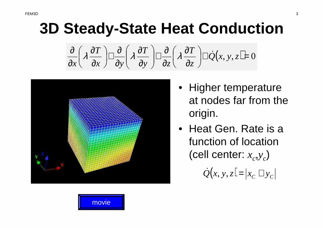
3D Steady -State Heat Conduction
• Higher temperature at nodes far from the origin.
• Heat Gen. Rate is a function of location (cell center: xc,yc)
movie
( ) 0,, =+
∂∂
∂∂+
∂∂
∂∂+
∂∂
∂∂
zyxQz
T
zy
T
yx
T
x&λλλ
( ) CC yxzyxQ +=,,&
FEM3D 3
Finite-Element Procedures
• Governing Equations• Galerkin Method: Weak Form• Element-by-Element Integration
– Element Matrix
• Global Matrix• Boundary Conditions• Linear Solver
FEM3D 4

FEM Procedures: Program
• Initialization– Control Data– Node, Connectivity of Elements (N: Node#, NE: Elem#)– Initialization of Arrays (Global/Element Matrices)– Element-Global Matrix Mapping (Index, Item)
• Generation of Matrix– Element-by-Element Operations (do icel= 1, NE)
• Element matrices• Accumulation to global matrix
– Boundary Conditions
• Linear Solver– Conjugate Gradient Method
FEM3D 5

• Formulation of 3D Element• 3D Heat Equations
– Galerkin Method– Element Matrices
• Running the Code• Data Structure• Overview of the Program
FEM3D 6

7
Extension to 2D Prob.: Triangles三角形要素
• Triangles can handle arbitrarily shaped object• “Linear” triangular elements provide low accuracy,
therefore they are not used in practical applications.
FEM3D

8
Extension to 2D Prob.: Quadrilaterals四角形要素
• Formulation of quad. elements is possible if same shape functions in 1D elements are applied along X-and Y- axis.– More accurate than triangles
• Each edge must be “parallel” with X- and Y- axis.– Similar to FDM
12
34
x
y • This type of elements cannot be considered.
FEM3D

9
Isoparametric Element (1/3)• Each element is mapped to square element [±1,±1]
on natural/local coordinate (ξ,η)
12
34
x
yη
ξ
1 2
4 3
-1
+1
+1-1
• Components of global coordinate system of each node (x,y) for certain kinds of elements are defined by shape functions [N] on natural/local coordinate system, where shape functions [N] are also used for interpolation of dependent variables.
FEM3D

10
Isoparametric Element (2/3)
12
34
x
y
• Coordinate of each node: (x1,y1), (x2,y2), (x3,y3), (x4,y4)
• Temperature at each node: T1, T2, T3, T4
η
ξ
4 3
-1
+1
+1-1
1 2
FEM3D
ii
iii
i
ii
i
yNyxNx
TNT
⋅=⋅=
⋅=
∑∑
∑
==
=
4
1
4
1
4
1
),(,),(
),(
ηξηξ
ηξ

11
Isoparametric Element (3/3)
x
y
• Higher-order shape function can handle curved lines/surfaces.
• “Natural” coordinate system
η
ξ
-1
+1
+1-1
FEM3D
Sub-ParametricSuper-Parametric

12
Shape Fn’s on 2D Natural Coord. (1/3)
• Polynomial shape functions on squares of natural coordinate:
ξηαηαξαα 4321 +++=T
• Coefficients are calculated as follows:
η
ξ
4
-1
+1
+1-1
3
1 2
FEM3D
4,
4
,4
,4
43214
43213
43212
43211
TTTTTTTT
TTTTTTTT
−+−=++−−=
−++−=+++=
αα
αα

Shape Fn’s on 2D Natural Coord. (2/3)η
ξ
4
-1
+1
+1-1
3
1 2
FEM3D 13
( ) ( )
( ) ( )
( )( ) ( )( )
( )( ) ( )( ) 43
21
43
21
43214321
43214321
4321
114
111
4
1
114
111
4
1
14
11
4
1
14
11
4
144
44
TT
TT
TT
TT
TTTTTTTT
TTTTTTTT
T
ηξηξ
ηξηξ
ξηηξξηηξ
ξηηξξηηξ
ξηη
ξ
ξηαηαξαα
+−+++
+−++−−=
−+−++++
+−−+++−−=
−+−+++−−
+−++−++++=
+++=
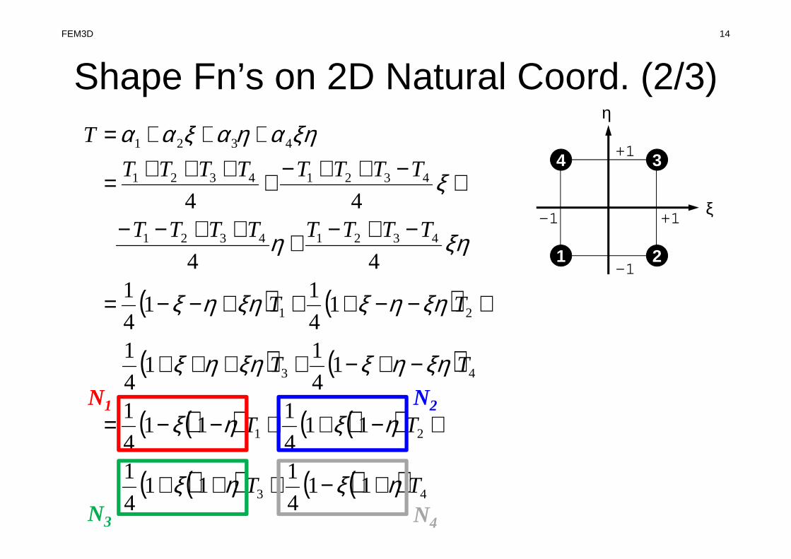
Shape Fn’s on 2D Natural Coord. (2/3)η
ξ
4
-1
+1
+1-1
3
1 2
FEM3D 14
( ) ( )
( ) ( )
( )( ) ( )( )
( )( ) ( )( ) 43
21
43
21
43214321
43214321
4321
114
111
4
1
114
111
4
1
14
11
4
1
14
11
4
144
44
TT
TT
TT
TT
TTTTTTTT
TTTTTTTT
T
ηξηξ
ηξηξ
ξηηξξηηξ
ξηηξξηηξ
ξηη
ξ
ξηαηαξαα
+−+++
+−++−−=
−+−++++
+−−+++−−=
−+−+++−−
+−++−++++=
+++=
N1 N2
N3 N4

15
Shape Fn’s on 2D Natural Coord. (3/3)
• T is defined as follows according to Ti :
( )( ) ( )( )
( )( ) ( )( )ηξηξηξηξ
ηξηξηξηξ
+−=++=
−+=−−=
114
1),(,11
4
1),(
,114
1),(,11
4
1),(
43
21
NN
NN
• Shape functions Ni :
• Also known as “bi-linear” interpolation• Calculate Ni at each node
η
ξ
-1
+1
+1-1
4 3
1 2
FEM3D
44332211 TNTNTNTNT +++=
16
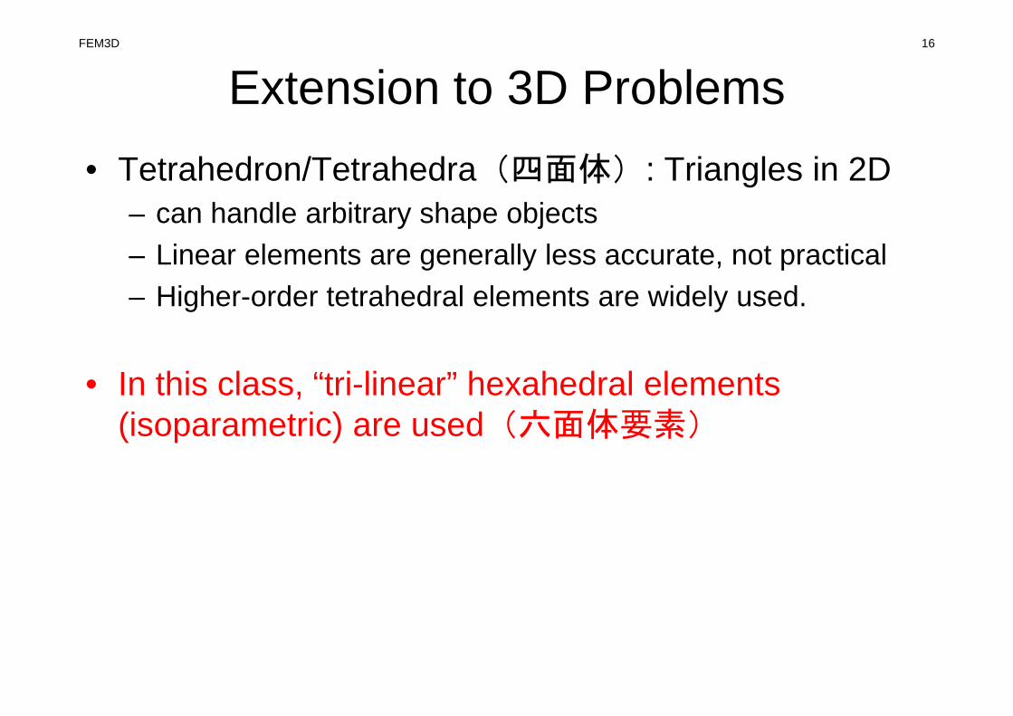
Extension to 3D Problems
• Tetrahedron/Tetrahedra(四面体): Triangles in 2D– can handle arbitrary shape objects– Linear elements are generally less accurate, not practical– Higher-order tetrahedral elements are widely used.
• In this class, “tri-linear” hexahedral elements (isoparametric) are used(六面体要素)
FEM3D

17
( )1,1,1 −+−
Shape Fn’s: 3D Natural/Local Coord.( )( )( )
( )( )( )
( )( )( )
( )( )( )ζηξζηξ
ζηξζηξ
ζηξζηξ
ζηξζηξ
−+−=
−++=
−−+=
−−−=
1118
1),,(
1118
1),,(
1118
1),,(
1118
1),,(
4
3
2
1
N
N
N
N
( ) ( )1,1,1,, −−−=ζηξ1 2
34
5 6
78
( )( )( )
( )( )( )
( )( )( )
( )( )( )ζηξζηξ
ζηξζηξ
ζηξζηξ
ζηξζηξ
++−=
+++=
+−+=
+−−=
1118
1),,(
1118
1),,(
1118
1),,(
1118
1),,(
8
7
6
5
N
N
N
N
( )1,1,1 −−+
( )1,1,1 −++
( )1,1,1 +−− ( )1,1,1 +−+
( )1,1,1 +++( )1,1,1 ++−
ii
i
ii
i
ii
iii
i
zNz
yNy
TNTxNx
⋅=
⋅=
⋅=⋅=
∑
∑
∑∑
=
=
==
8
1
8
1
8
1
8
1
),,(
),,(
),,(,),,(
ζηξ
ζηξ
ζηξζηξ
FEM3D
• Formulation of 3D Element• 3D Heat Equations
– Galerkin Method– Element Matrices
• Running the Code• Data Structure• Overview of the Program
FEM3D 18

Galerkin Method (1/3)
• Governing Equation for 3D Steady State Heat Conduction Problems (uniform λ):
[ ] }{φNT =
• Following integral equation is obtained at each element by Galerkin method, where [N]’s are also weighting functions:
[ ] 02
2
2
2
2
2
=
+
∂∂+
∂∂+
∂∂
∫ dVQz
T
y
T
x
TN
T
V
&λλλ
02
2
2
2
2
2
=+
∂∂+
∂∂+
∂∂
Qz
T
y
T
x
T&λλλ
FEM3D 19
Distribution of temperature in each element (matrix form), φ: Temperature at each node
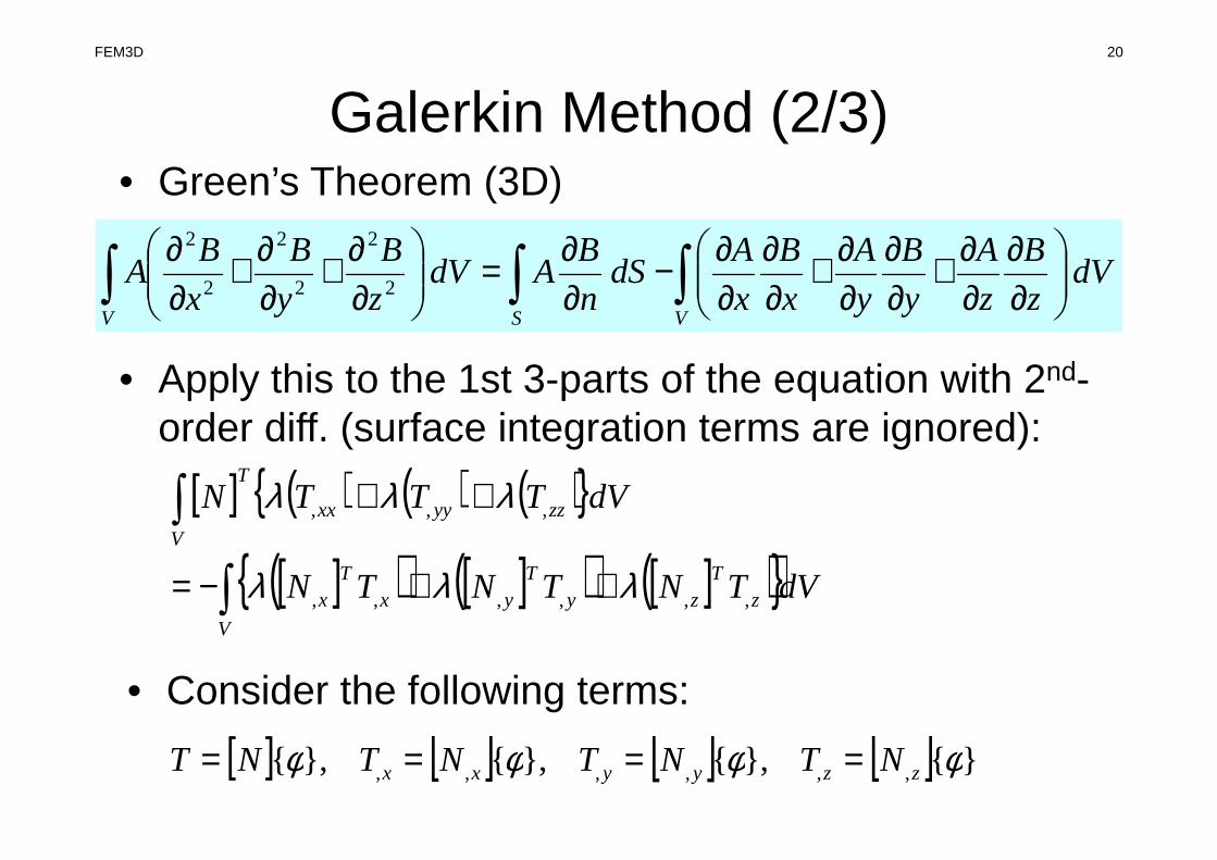
Galerkin Method (2/3)• Green’s Theorem (3D)
• Apply this to the 1st 3-parts of the equation with 2nd-order diff. (surface integration terms are ignored):
• Consider the following terms:
[ ] [ ] [ ] [ ] }{},{},{},{ ,,,,,, φφφφ zzyyxx NTNTNTNT ====
∫∫ ∫
∂∂
∂∂+
∂∂
∂∂+
∂∂
∂∂−
∂∂=
∂∂+
∂∂+
∂∂
VV S
dVz
B
z
A
y
B
y
A
x
B
x
AdS
n
BAdV
z
B
y
B
x
BA
2
2
2
2
2
2
[ ] ( ) ( ) ( ){ }
[ ]( ) [ ]( ) [ ]( ){ }dVTNTNTN
dVTTTN
V
zT
zyT
yxT
x
zzyyxx
T
V
∫
∫
++−=
++
,,,,,,
,,,
λλλ
λλλ
FEM3D 20

Galerkin Method (3/3)• Finally, following equation is obtained by considering
heat generation term :
• This is called “weak form(弱形式)”. Original PDE consists of terms with 2nd-order diff., but this “weak form” only includes 1st-order diff by Green’s theorem.– Requirements for shape functions are “weaker” in “weak
form”. Linear functions can describe effects of 2nd-order differentiation.
– Same as 1D problem
Q&
FEM3D 21
[ ] [ ]( ) [ ] [ ]( ) [ ] [ ]( ){ } { } [ ] 0,,,,,, =+⋅++− ∫∫ dVNQdVNNNNNNVV
zT
zyT
yxT
x&φλλλ

Weak Form with B.C.: on each elem.
[ ] [ ] [ ]( ) [ ] [ ]( )[ ] [ ]( )dVNN
dVNNdVNNk
V
zT
z
V
yT
y
V
xT
xe
∫
∫∫
+
+=
,,
,,,,)(
λ
λλ
[ ] { } { } )()()( eee fk =φ
[ ] [ ] dVNQfV
Te
∫= &
)(
FEM3D 22

Element Matrix: 8x8
( )1,1,1 −+−
( ) ( )1,1,1,, −−−=ζηξ1 2
34
5 6
78
( )1,1,1 −−+
( )1,1,1 −++
( )1,1,1 +−− ( )1,1,1 +−+
( )1,1,1 +++( )1,1,1 ++−
i
j
[ ] ( )81, K=jikij
FEM3D 23

Element Matrix: kij
( )1,1,1 −+−
( ) ( )1,1,1,, −−−=ζηξ1 2
34
5 6
78
( )1,1,1 −−+
( )1,1,1 −++
( )1,1,1 +−− ( )1,1,1 +−+
( )1,1,1 +++( )1,1,1 ++−[ ] ( )81, K=jikij
{ }∫ ⋅⋅+⋅⋅+⋅⋅−=V
zjziyjyixjxiij dVNNNNNNk ,,,,,, λλλ
[ ] [ ] [ ]( ) [ ] [ ]( )[ ] [ ]( )dVNN
dVNNdVNNk
V
zT
z
V
yT
y
V
xT
xe
∫
∫∫
+
+=
,,
,,,,)(
λ
λλ
FEM3D 24

Next Stage: IntegrationFEM3D 25
FEM3D 26
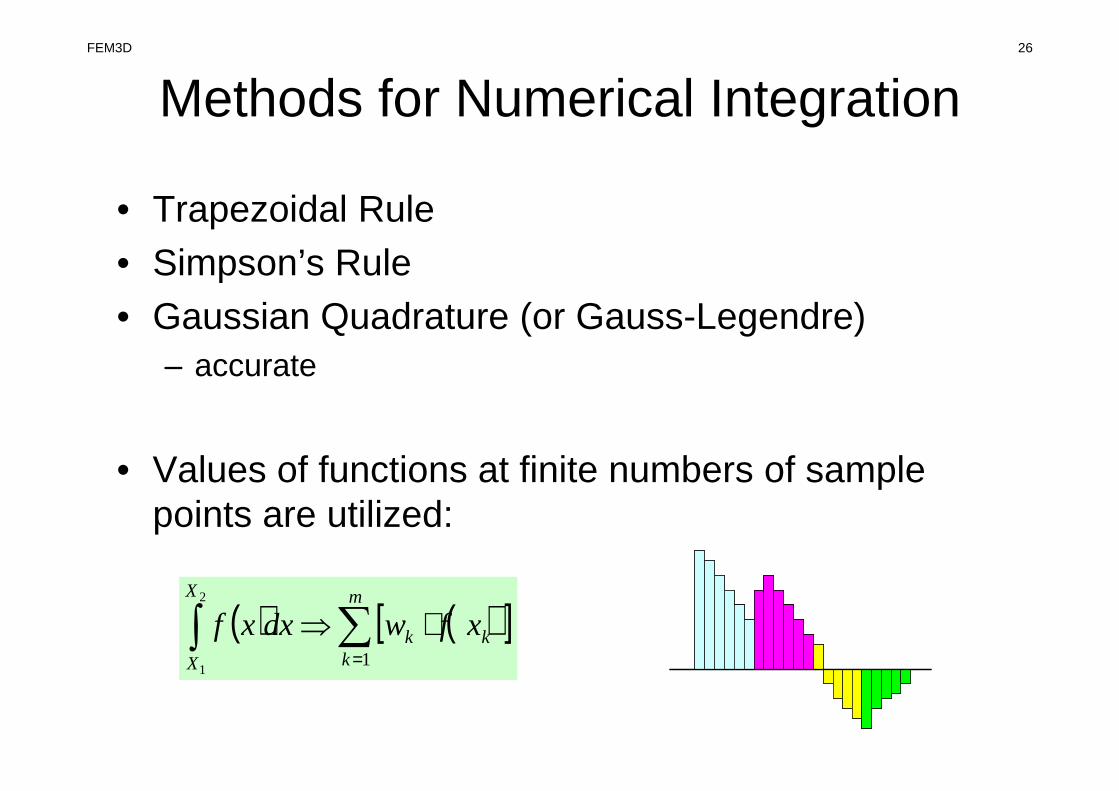
Methods for Numerical Integration
• Trapezoidal Rule• Simpson’s Rule• Gaussian Quadrature (or Gauss-Legendre)
– accurate
• Values of functions at finite numbers of sample points are utilized:
( ) ( )[ ]∑∫=
⋅⇒m
kkk
X
X
xfwdxxf1
2
1
FEM3D 27
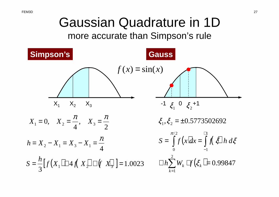
Gaussian Quadrature in 1D more accurate than Simpson’s rule
)sin()( xxf =
X1 X2 X3
2,
4,0 321
ππ === XXX
41312
π=−=−= XXXXh
( ) ( ) ( )[ ] 0023.143 321 =++= XfXfXfh
S
-1 0 +11ξ 2ξ
( ) ( )
( ) 99847.02
1
1
1
2/
0
=⋅≅
==
∑
∫∫
=
+
−
kk
k fWh
dhfdxxfS
ξ
ξξπ
5773502692.0, 21 ±=ξξ
Simpson’s Gauss

FEM3D 28
Gaussian Quadratureガウスの積分公式
• On normalized “natural (or local)” coordinate system [-1,+1](自然座標系,局所座標系)
• Can approximate up to (2m-1)-th order of functions by m quadrature points (m=2 is enough for quadratic shape functions).
( ) ( )[ ]∑∫=
+
−
⋅=m
kkk fwdf
1
1
1
ξξξξ=+1ξ=-1 ξ=0
ξk=-0.577350 ξk=+0.577350
9/5,774597.0
9/8,00.03
00.1,577350.02
00.2,00.01
=±====
=±=====
kk
kk
kk
kk
w
wm
wm
wm
ξξξξ

FEM3D 29
Gaussian Quadraturecan be easily extended to 2D & 3D
[ ]∑∑
∫∫
==
+
−
+
−
⋅⋅=
=
n
jjiji
m
i
fWW
ddfI
11
1
1
1
1
),(
),(
ηξ
ηξηξ
ji WW ,
),( ji ηξ
m,n: number of quadraturepoints in ξ,η-direction
:Weighting Factor
: Coordinates of Quad’s
30
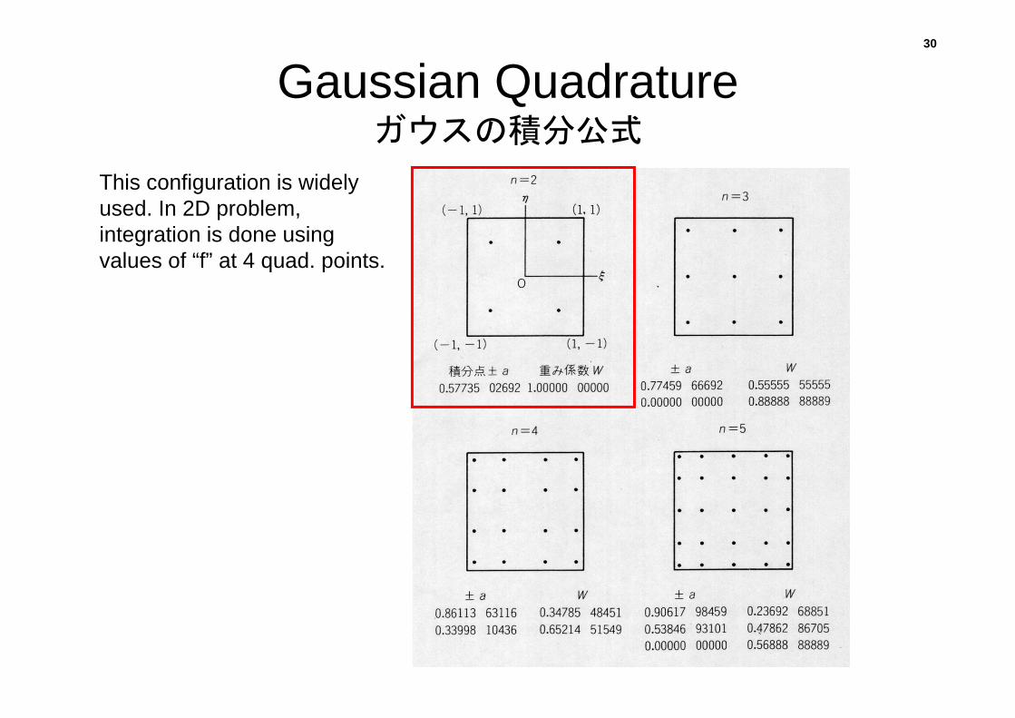
Gaussian Quadratureガウスの積分公式
This configuration is widely used. In 2D problem, integration is done using values of “f” at 4 quad. points.

31
Gaussian Quadratureガウスの積分公式
[ ]
)57735.0,57735.0(0.10.1)57735.0,57735.0(0.10.1
)57735.0,57735.0(0.10.1)57735.0,57735.0(0.10.1
),(),(11
1
1
1
1
−+××+++××++−××+−−××=
⋅⋅== ∑∑∫∫==
+
−
+
−
ff
ff
fWWddfIn
j
jiji
m
i
ηξηξηξ
This configuration is widely used. In 2D problem, integration is done using values of “f” at 4 quad. points.
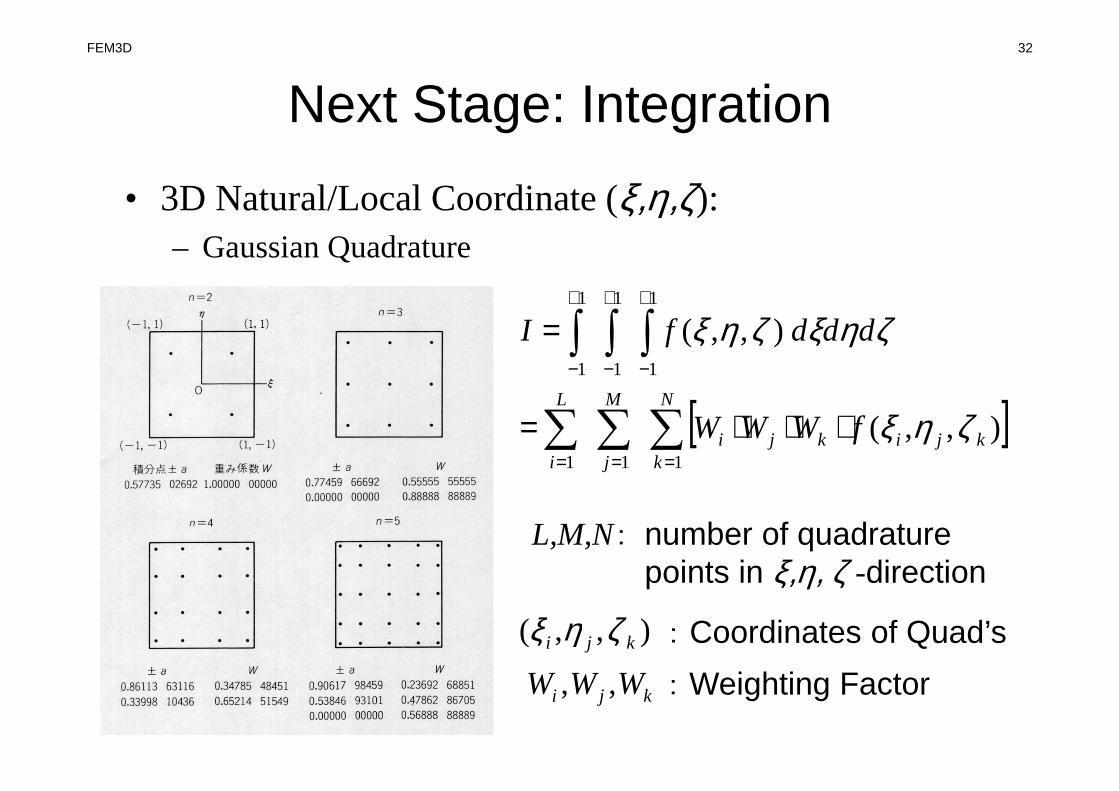
Next Stage: IntegrationFEM3D 32
• 3D Natural/Local Coordinate (ξ,η,ζ): – Gaussian Quadrature
kji WWW ,,
),,( kji ζηξ
[ ]∑∑∑
∫∫∫
===
+
−
+
−
+
−
⋅⋅⋅=
=
N
kkjikji
M
j
L
i
fWWW
dddfI
111
1
1
1
1
1
1
),,(
),,(
ζηξ
ζηξζηξ
L,M,N: number of quadraturepoints in ξ,η, ζ -direction
:Weighting Factor
: Coordinates of Quad’s
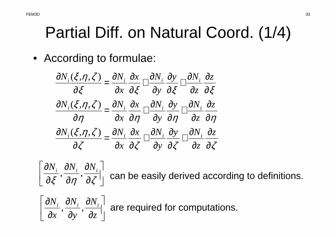
Partial Diff. on Natural Coord. (1/4)
• According to formulae:
ζζζζζηξ
ηηηηζηξ
ξξξξζηξ
∂∂
∂∂+
∂∂
∂∂+
∂∂
∂∂=
∂∂
∂∂
∂∂+
∂∂
∂∂+
∂∂
∂∂=
∂∂
∂∂
∂∂+
∂∂
∂∂+
∂∂
∂∂=
∂∂
z
z
Ny
y
Nx
x
NN
z
z
Ny
y
Nx
x
NN
z
z
Ny
y
Nx
x
NN
iiii
iiii
iiii
),,(
),,(
),,(
∂∂
∂∂
∂∂
ζηξiii NNN
,,
∂∂
∂∂
∂∂
z
N
y
N
x
N iii ,,
can be easily derived according to definitions.
are required for computations.
FEM3D 33

Partial Diff. on Natural Coord. (2/4)
• In matrix form:
[ ]
∂∂∂
∂∂
∂
=
∂∂∂
∂∂
∂
∂∂
∂∂
∂∂
∂∂
∂∂
∂∂
∂∂
∂∂
∂∂
=
∂∂∂∂∂∂
z
Ny
Nx
N
J
z
Ny
Nx
N
zyx
zyx
zyx
N
N
N
i
i
i
i
i
i
i
i
i
ζζζ
ηηη
ξξξ
ζ
η
ξ
[ ]J : Jacobi matrix, Jacobian
FEM3D 34

Partial Diff. on Natural Coord. (3/4)• Components of Jacobian:
ii
ii
ii
ii
ii
iii
i
ii
ii
ii
ii
ii
ii
ii
iii
i
ii
ii
ii
ii
ii
ii
ii
iii
i
ii
ii
zN
zNz
J
yN
yNy
JxN
xNx
J
zN
zNz
J
yN
yNy
JxN
xNx
J
zN
zNz
J
yN
yNy
JxN
xNx
J
∑∑
∑∑∑∑
∑∑
∑∑∑∑
∑∑
∑∑∑∑
==
====
==
====
==
====
∂∂=
∂∂=
∂∂=
∂∂=
∂∂=
∂∂=
∂∂=
∂∂=
∂∂=
∂∂=
∂∂=
∂∂=
∂∂=
∂∂=
∂∂=
∂∂=
∂∂=
∂∂=
∂∂=
∂∂=
∂∂=
∂∂=
∂∂=
∂∂=
∂∂=
∂∂=
∂∂=
8
1
8
133
8
1
8
132
8
1
8
131
8
1
8
123
8
1
8
122
8
1
8
121
8
1
8
113
8
1
8
112
8
1
8
111
,,
,,
,,
ζζζ
ζζζζζζ
ηηη
ηηηηηη
ξξξ
ξξξξξξ
FEM3D 35
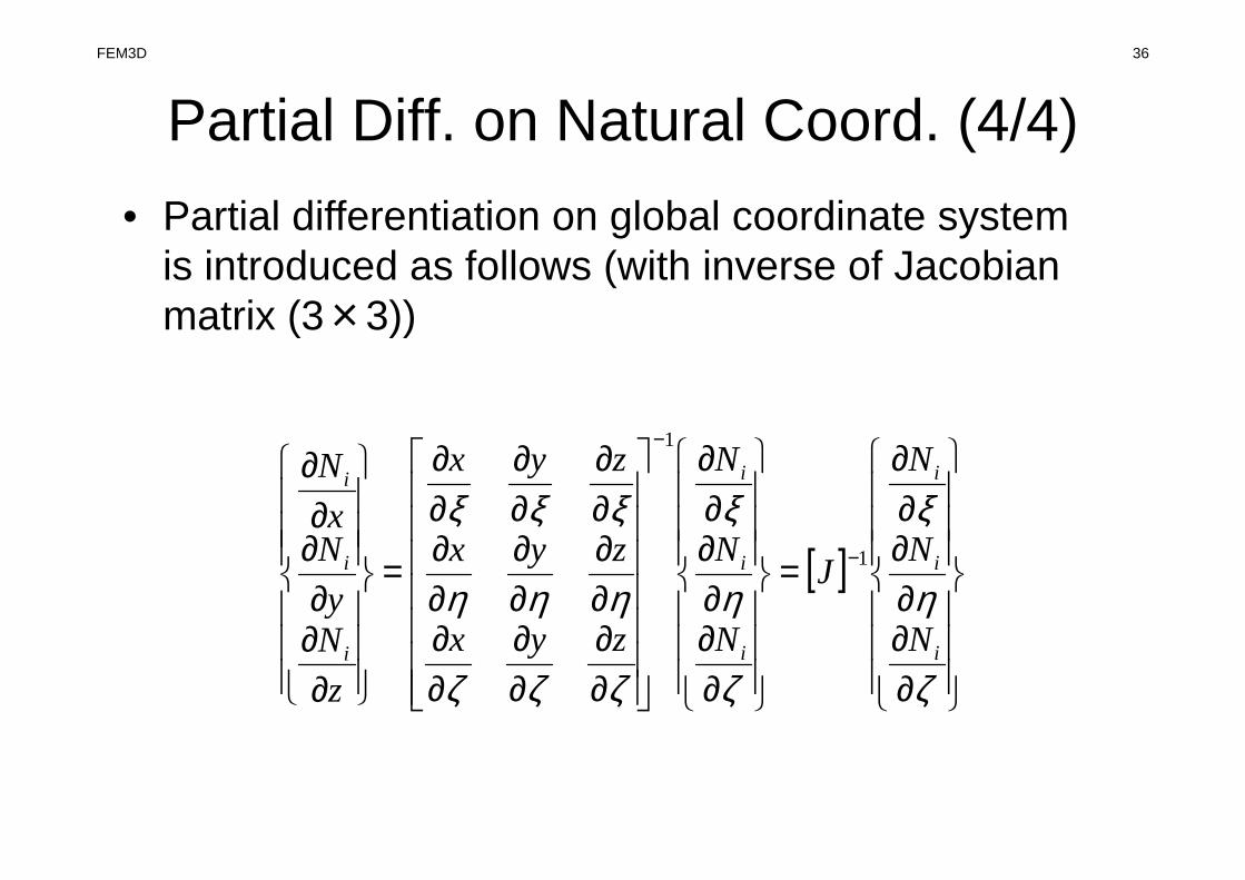
Partial Diff. on Natural Coord. (4/4)
• Partial differentiation on global coordinate system is introduced as follows (with inverse of Jacobianmatrix (3×3))
[ ]
∂∂∂∂∂∂
=
∂∂∂∂∂∂
∂∂
∂∂
∂∂
∂∂
∂∂
∂∂
∂∂
∂∂
∂∂
=
∂∂∂
∂∂
∂
−
−
ζ
η
ξ
ζ
η
ξ
ζζζ
ηηη
ξξξ
i
i
i
i
i
i
i
i
i
N
N
N
J
N
N
N
zyx
zyx
zyx
z
Ny
Nx
N
1
1
FEM3D 36
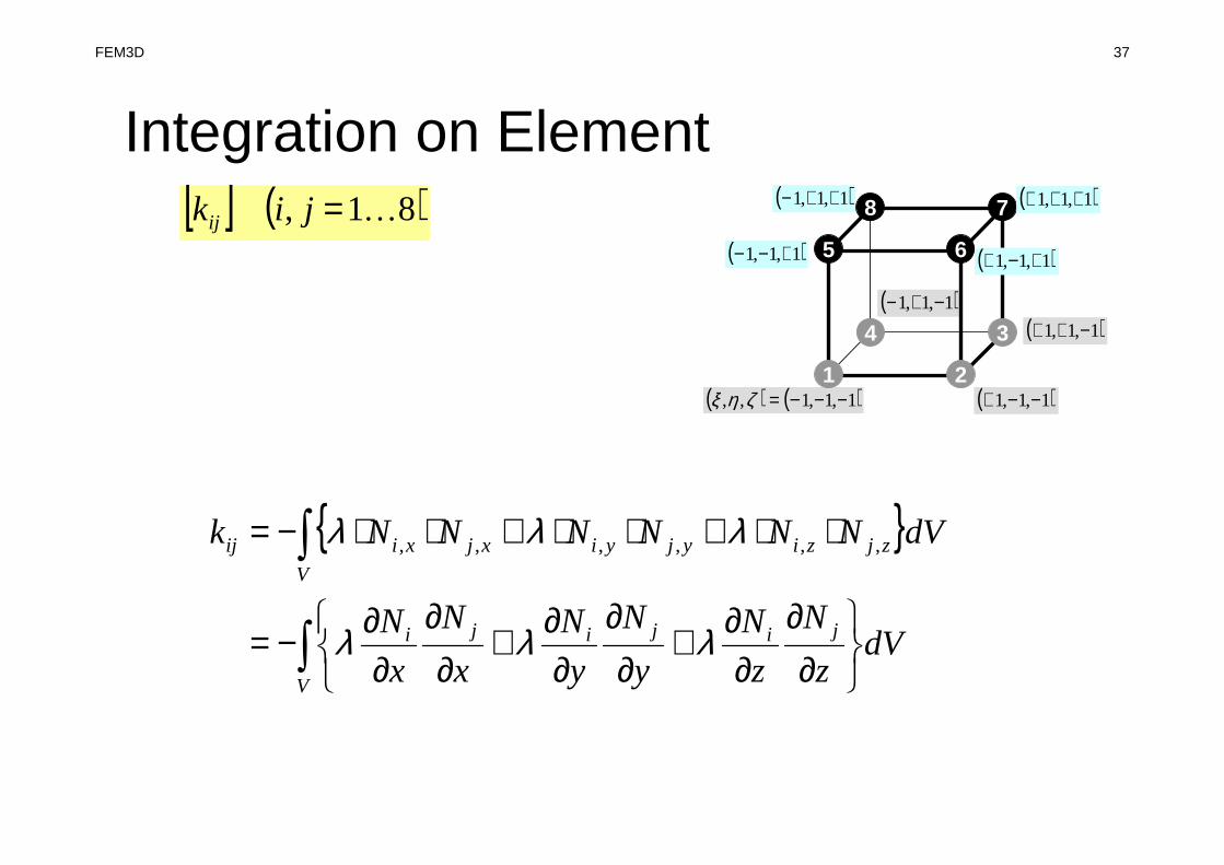
Integration on Element
{ }
∫
∫
∂∂
∂∂+
∂∂
∂∂+
∂∂
∂∂−=
⋅⋅+⋅⋅+⋅⋅−=
V
jijiji
V
zjziyjyixjxiij
dVz
N
z
N
y
N
y
N
x
N
x
N
dVNNNNNNk
λλλ
λλλ ,,,,,,
( )1,1,1 −+−
( ) ( )1,1,1,, −−−=ζηξ1 2
34
5 6
78
( )1,1,1 −−+
( )1,1,1 −++
( )1,1,1 +−− ( )1,1,1 +−+
( )1,1,1 +++( )1,1,1 ++−[ ] ( )81, K=jikij
FEM3D 37
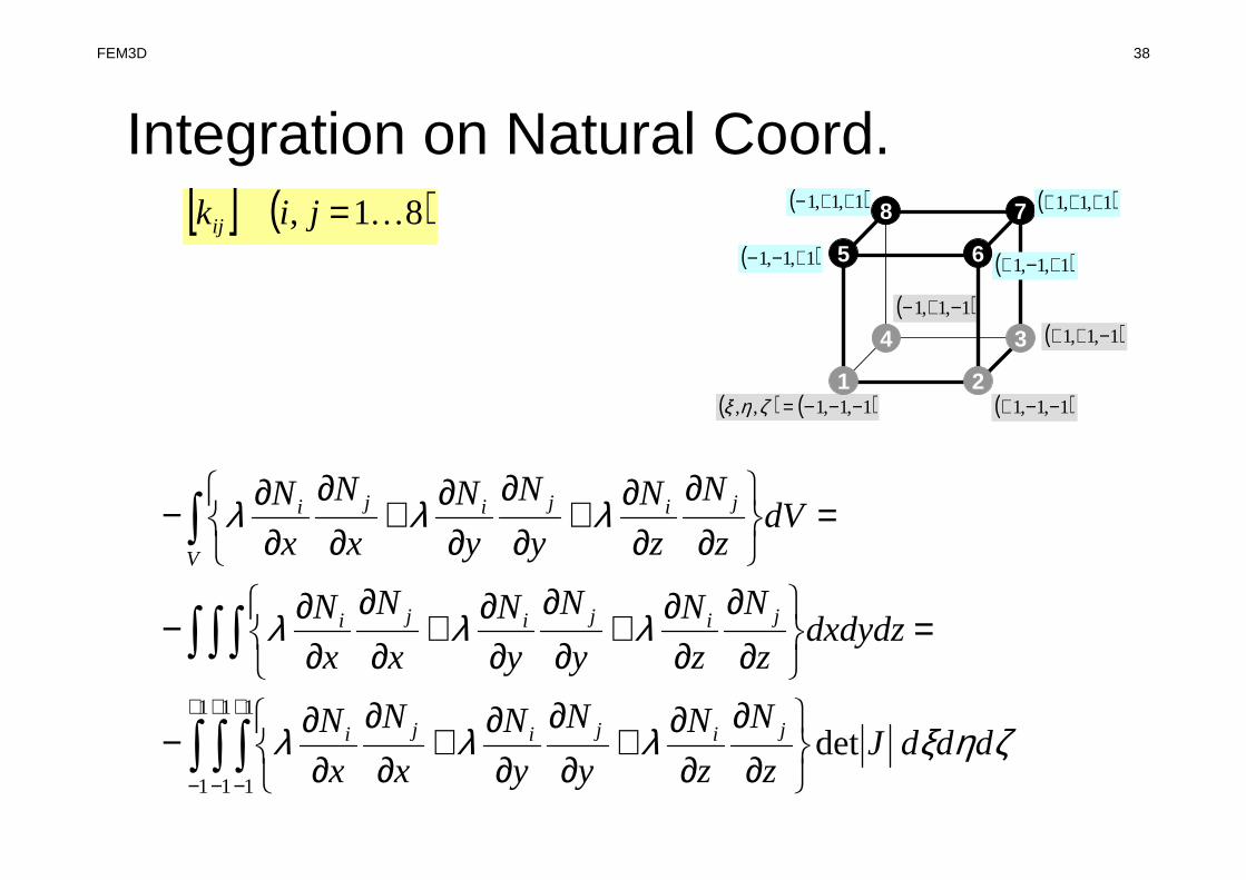
Integration on Natural Coord.
ζηξλλλ
λλλ
λλλ
dddJz
N
z
N
y
N
y
N
x
N
x
N
dxdydzz
N
z
N
y
N
y
N
x
N
x
N
dVz
N
z
N
y
N
y
N
x
N
x
N
jijiji
jijiji
V
jijiji
det1
1
1
1
1
1∫ ∫ ∫
∫ ∫ ∫
∫
+
−
+
−
+
−
∂∂
∂∂+
∂∂
∂∂+
∂∂
∂∂−
=
∂∂
∂∂+
∂∂
∂∂+
∂∂
∂∂−
=
∂∂
∂∂+
∂∂
∂∂+
∂∂
∂∂−
( )1,1,1 −+−
( ) ( )1,1,1,, −−−=ζηξ1 2
34
5 6
78
( )1,1,1 −−+
( )1,1,1 −++
( )1,1,1 +−− ( )1,1,1 +−+
( )1,1,1 +++( )1,1,1 ++−[ ] ( )81, K=jikij
FEM3D 38

Gaussian Quadrature
( )1,1,1 −+−
( ) ( )1,1,1,, −−−=ζηξ1 2
34
5 6
78
( )1,1,1 −−+
( )1,1,1 −++
( )1,1,1 +−− ( )1,1,1 +−+
( )1,1,1 +++( )1,1,1 ++−
[ ]∑∑∑
∫∫∫
===
+
−
+
−
+
−
⋅⋅⋅=
=
N
kkjikji
M
j
L
i
fWWW
dddfI
111
1
1
1
1
1
1
),,(
),,(
ζηξ
ζηξζηξ
ζηξλλλ dddJz
N
z
N
y
N
y
N
x
N
x
N jijiji det1
1
1
1
1
1∫ ∫ ∫+
−
+
−
+
−
∂∂
∂∂+
∂∂
∂∂+
∂∂
∂∂−
FEM3D 39
[ ] ( )81, K=jikij

Remaining Procedures
• Element matrices have been formed.
• Accumulation to Global Matrix• Implementation of Boundary Conditions• Solving Linear Equations
• Details of implementation will be discussed in classes later than next week through explanation of programs
FEM3D 40

Accumulation: Local -> Global Matrices
1
2
4
5 6
3
1 22
34
1 2
1
2
4 3
1
=
=
)1(4
)1(3
)1(2
)1(1
)1(4
)1(3
)1(2
)1(1
)1(44
)1(43
)1(42
)1(41
)1(34
)1(33
)1(32
)1(31
)1(24
)1(23
)1(22
)1(21
)1(14
)1(13
)1(12
)1(11
)1()1()1( }{}]{[
f
f
f
f
kkkk
kkkk
kkkk
kkkk
fk
φφφφ
φ
=
=
)2(4
)2(3
)2(2
)2(1
)2(4
)2(3
)2(2
)2(1
)2(44
)2(43
)2(42
)2(41
)2(34
)2(33
)2(32
)2(31
)2(24
)2(23
)2(22
)2(21
)2(14
)2(13
)2(12
)2(11
)2()2()2( }{}]{[
f
f
f
f
kkkk
kkkk
kkkk
kkkk
fk
φφφφ
φ
=
ΦΦΦΦΦΦ
=Φ
6
5
4
3
2
1
6
5
4
3
2
1
6
5
4
3
2
1
}{}]{[
B
B
B
B
B
B
DXXX
XDXX
XXDXXX
XXXDXX
XXDX
XXXD
FK
FEM3D 41
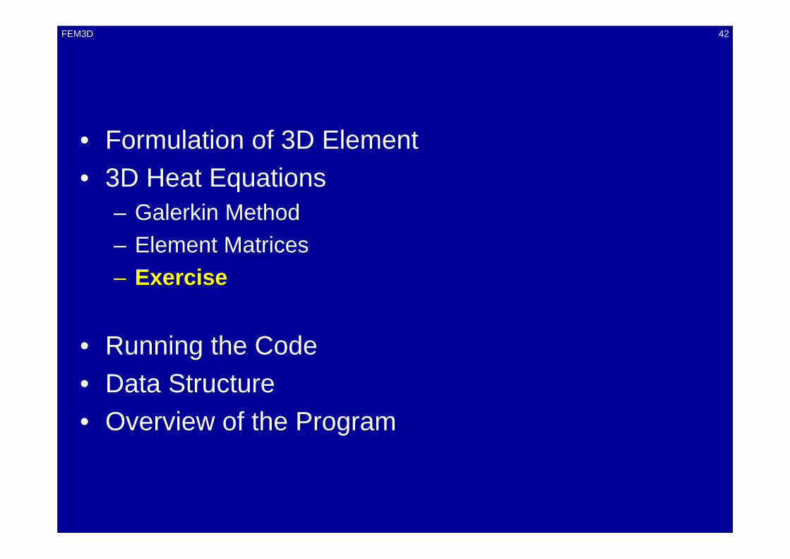
• Formulation of 3D Element• 3D Heat Equations
– Galerkin Method– Element Matrices– Exercise
• Running the Code• Data Structure• Overview of the Program
FEM3D 42

Exercise• Develop a program and calculate area of the following
quadrilateral using Gaussian Quadrature.
1
2
34
x
y
V1:(1.0, 1.0)2:(4.0, 2.0)3:(3.0, 5.0)4:(2.0, 4.0)
ζξddJdVIV
∫∫∫+
−
+
−
==1
1
1
1
det
FEM3D 43

FEM3D 44
Tips (1/2)
• Calculate Jacobian
• Apply Gaussian Quadrature (n=2)
[ ]∑∑∫∫==
+
−
+
−
⋅⋅==n
j
jiji
m
i
fWWddfI11
1
1
1
1
),(),( ηξηξηξ
implicit REAL*8 (A-H,O-Z)real*8 W(2)real*8 POI(2)
W(1)= 1.0d0W(2)= 1.0d0POI(1)= -0.5773502692d0POI(2)= +0.5773502692d0
SUM= 0.d0do jp= 1, 2do ip= 1, 2FC = F(POI(ip),POI(jp))SUM= SUM + W (ip)*W (jp)*FC
enddoenddo

FEM3D 45
Tips (2/2)
[ ]ηξηξ
ηη
ξξ∂∂⋅
∂∂−
∂∂⋅
∂∂=
∂∂
∂∂
∂∂
∂∂
= xyyxJ
yx
yx
J det,
( )( ) ( )( )
( )( ) ( )( )ηξηξηξηξ
ηξηξηξηξ
+−=++=
−+=−−=
114
1),(,11
4
1),(
,114
1),(,11
4
1),(
43
21
NN
NN
ii
ii
iii
i
ii
ii
ii
ii
iii
i
ii
ii
yN
yNy
xN
xNx
yN
yNy
xN
xNx
∑∑∑∑
∑∑∑∑
====
====
∂∂=
∂∂=
∂∂
∂∂=
∂∂=
∂∂
∂∂=
∂∂=
∂∂
∂∂=
∂∂=
∂∂
4
1
4
1
4
1
4
1
4
1
4
1
4
1
4
1
,
,,
ηηηηηη
ξξξξξξ

• Formulation of 3D Element• 3D Heat Equations
– Galerkin Method– Element Matrices
• Running the Code• Data Structure• Overview of the Program
FEM3D 46

3D Steady -State Heat Conduction
• Heat Generation• Uniform thermal conductivity λ
• HEX meshes– 1x1x1 cubes– NX, NY, NZ cubes in each direction
• Boundary Conditions– T=0@Z=zmax
• Heat Gen. Rate is a function of location (cell center: xc,yc)– ( ) CC yxQVOLzyxQ +=,,&
( ) 0,, =+
∂∂
∂∂+
∂∂
∂∂+
∂∂
∂∂
zyxQz
T
zy
T
yx
T
x&λλλ
X
Y
Z
NYNX
NZ
T=0@Z=zmax
FEM3D 47

Copy/Installation
Install
>$ cd <$E-TOP>/fem-f/fem3d/src>$ make>$ ls ../run/sol
sol
Install of Mesh Generator
>$ cd <$E-TOP>/fem-f/fem3d/run>$ gfortran –O3 mgcube.f –o mgcube
FEM3D 48

OperationsStarting from Grid Generation to Computation, File-
names are fixed
FEM3D 49
mgcubemesh generator
solFEM Solver
cube.0mesh file
test.inpfor visualization
INPUT.DATControl Data
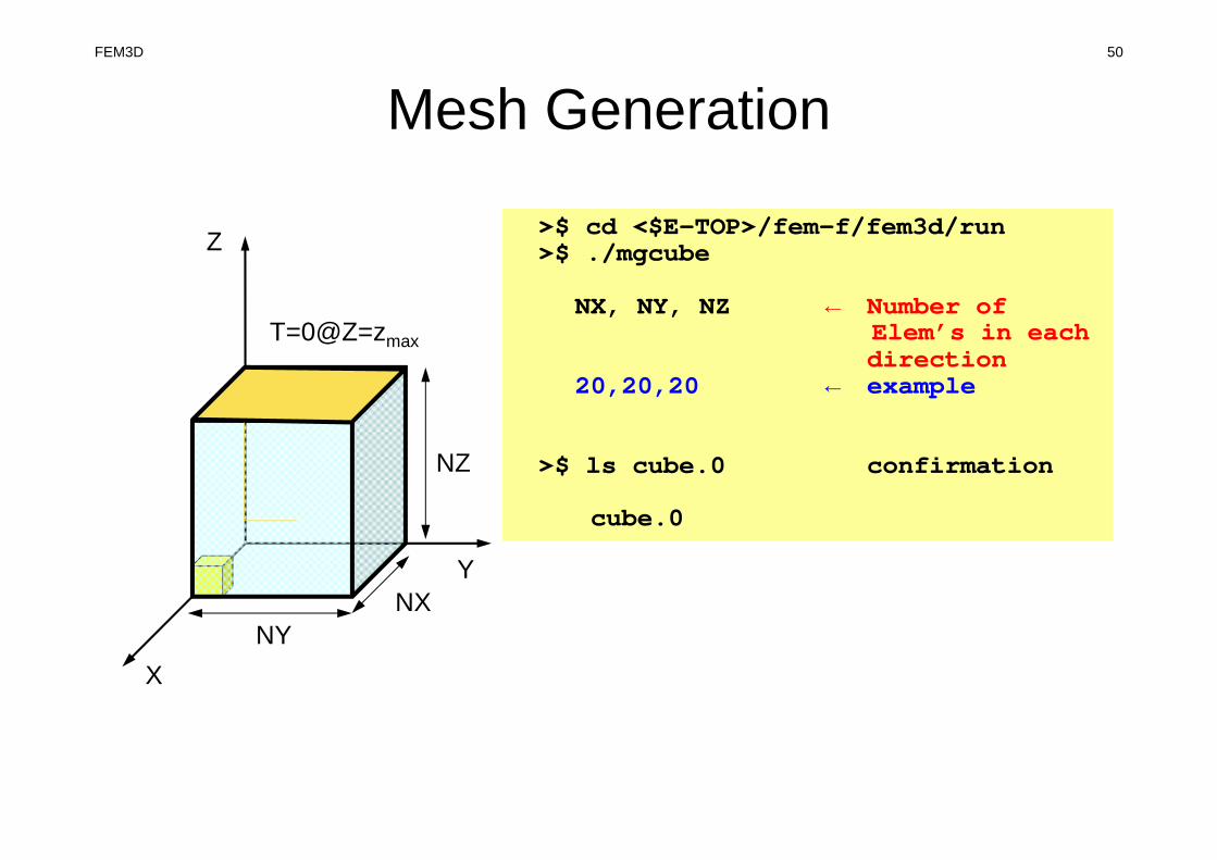
Mesh Generation
X
Y
Z
NYNX
NZ
T=0@Z=zmax
FEM3D 50
>$ cd <$E-TOP>/fem-f/fem3d/run>$ ./mgcube
NX, NY, NZ ← Number of Elem’s in eachdirection
20,20,20 ← example
>$ ls cube.0 confirmation
cube.0
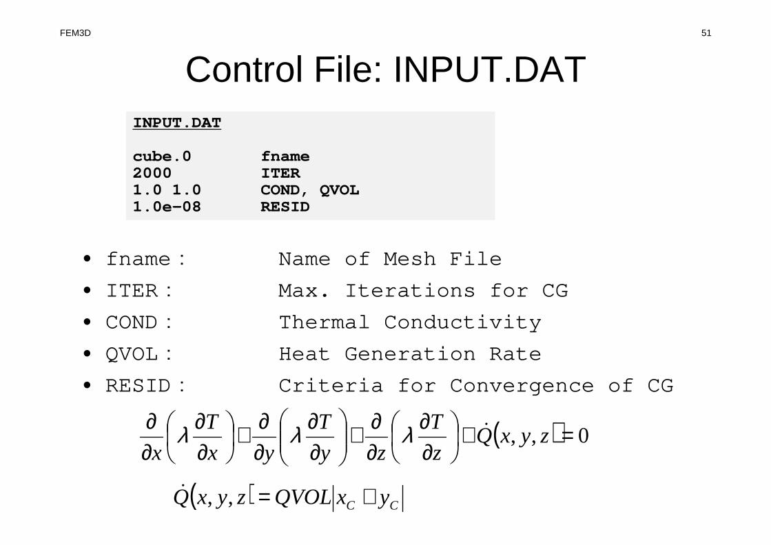
Control File: INPUT.DATINPUT.DAT
cube.0 fname2000 ITER1.0 1.0 COND, QVOL1.0e-08 RESID
• fname: Name of Mesh File
• ITER: Max. Iterations for CG
• COND: Thermal Conductivity
• QVOL: Heat Generation Rate
• RESID: Criteria for Convergence of CG
( ) 0,, =+
∂∂
∂∂+
∂∂
∂∂+
∂∂
∂∂
zyxQz
T
zy
T
yx
T
x&λλλ
( ) CC yxQVOLzyxQ +=,,&
FEM3D 51
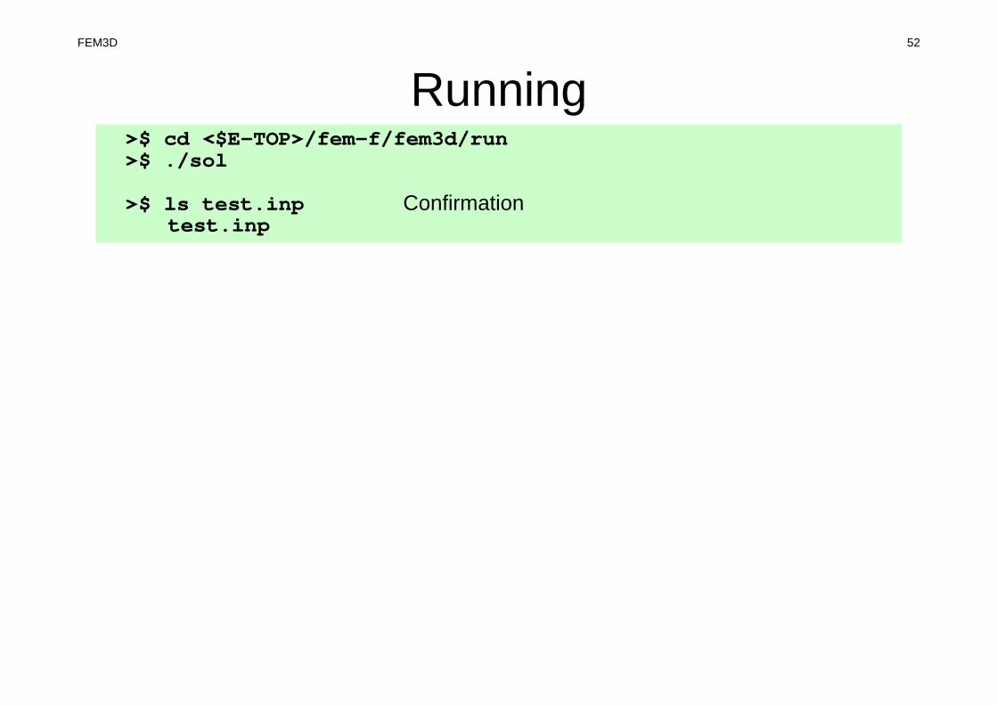
Running>$ cd <$E-TOP>/fem-f/fem3d/run>$ ./sol
>$ ls test.inp Confirmationtest.inp
FEM3D 52

ParaView
• http://www.paraview.org/
• Opening files• Displaying figures• Saving image files
– http://nkl.cc.u-tokyo.ac.jp/class/HowtouseParaViewE.pdf– http://nkl.cc.u-tokyo.ac.jp/class/HowtouseParaViewJ.pdf
FEM3D 53

UCD Format (1/3)Unstructured Cell Data
要素の種類 キーワード
点 pt
線 line
三角形 tri
四角形 quad
四面体 tet
角錐 pyr
三角柱 prism
六面体 hex
二次要素
線2 line2
三角形2 tri2
四角形2 quad2
四面体2 tet2
角錐2 pyr2
三角柱2 prism2
六面体2 hex2
FEM3D 54

UCD Format (2/3)
• Originally for AVS, microAVS• Extension of the UCD file is “inp”• There are two types of formats. Only old type can
be read by ParaView.
FEM3D 55

UCD Format (3/3): Old Format(全節点数) (全要素数) (各節点のデータ数) (各要素のデータ数) (モデルのデータ数)(節点番号1) (X座標) (Y座標) (Z座標) (節点番号2) (X座標) (Y座標) (Z座標)
・・・
(要素番号1) (材料番号) (要素の種類) (要素を構成する節点のつながり) (要素番号2) (材料番号) (要素の種類) (要素を構成する節点のつながり)
・・・
(節点のデータ成分数) (成分1の構成数) (成分2の構成数) ・・・(各成分の構成数)(節点データ成分1のラベル),(単位)(節点データ成分2のラベル),(単位)
・・・
(各節点データ成分のラベル),(単位)(節点番号1) (節点データ1) (節点データ2) ・・・・・(節点番号2) (節点データ1) (節点データ2) ・・・・・
・・・
(要素のデータ成分数) (成分1の構成数) (成分2の構成数) ・・・(各成分の構成数)(要素データ成分1のラベル),(単位)(要素データ成分2のラベル),(単位)
・・・
(各要素データ成分のラベル),(単位)(要素番号1) (要素データ1) (要素データ2) ・・・・・(要素番号2) (要素データ1) (要素データ2) ・・・・・
・・・
FEM3D 56

• Formulation of 3D Element• 3D Heat Equations
– Galerkin Method– Element Matrices
• Running the Code• Data Structure• Overview of the Program
FEM3D 57

Overview of Mesh File: cube.0numbering starts from “1”
• Nodes– Node # (How many nodes ?)– Node ID, Coordinates
• Elements– Element #– Element Type– Element ID, Material ID, Connectivity
• Node Groups– Group #– Node # in each group– Group Name– Nodes in each group
FEM3D 58

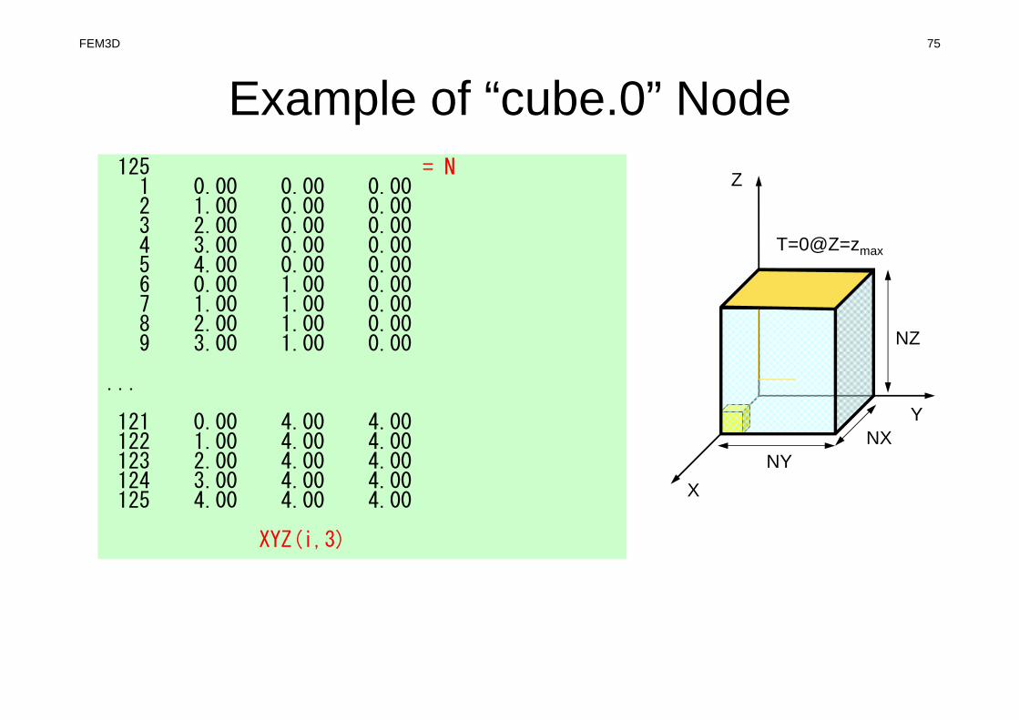
Example of “cube.0” (NX=NY=NZ=4)Node
125 =5*5*5 (Node #)1 0.00 0.00 0.002 1.00 0.00 0.003 2.00 0.00 0.004 3.00 0.00 0.005 4.00 0.00 0.006 0.00 1.00 0.007 1.00 1.00 0.008 2.00 1.00 0.009 3.00 1.00 0.00
...
121 0.00 4.00 4.00122 1.00 4.00 4.00123 2.00 4.00 4.00124 3.00 4.00 4.00125 4.00 4.00 4.00
Node ID X-coord. Y Z
movie
FEM3D 59
X
Y
Z
NYNX
NZ
T=0@Z=zmax

Example of “cube.0” (NX=NY=NZ=4)Element (1/2)
FEM3D 60
64 =4*4*4 (Element #)361 361 361 361 361 361 361 361 361 361361 361 361 361 361 361 361 361 361 361361 361 361 361 361 361 361 361 361 361361 361 361 361 361 361 361 361 361 361361 361 361 361 361 361 361 361 361 361361 361 361 361 361 361 361 361 361 361361 361 361 361
X
Y
Z
NYNX
NZ
T=0@Z=zmax
Element Type: 3613D, Hexahedron, Linear (1st order)

Example of “cube.0” Element (2/2)1 1 1 2 7 6 26 27 32 312 1 2 3 8 7 27 28 33 323 1 3 4 9 8 28 29 34 334 1 4 5 10 9 29 30 35 345 1 6 7 12 11 31 32 37 366 1 7 8 13 12 32 33 38 377 1 8 9 14 13 33 34 39 388 1 9 10 15 14 34 35 40 399 1 11 12 17 16 36 37 42 41
10 1 12 13 18 17 37 38 43 4211 1 13 14 19 18 38 39 44 4312 1 14 15 20 19 39 40 45 4413 1 16 17 22 21 41 42 47 46
...53 1 81 82 87 86 106 107 112 11154 1 82 83 88 87 107 108 113 11255 1 83 84 89 88 108 109 114 11356 1 84 85 90 89 109 110 115 11457 1 86 87 92 91 111 112 117 11658 1 87 88 93 92 112 113 118 11759 1 88 89 94 93 113 114 119 11860 1 89 90 95 94 114 115 120 11961 1 91 92 97 96 116 117 122 12162 1 92 93 98 97 117 118 123 12263 1 93 94 99 98 118 119 124 12364 1 94 95 100 99 119 120 125 124
Elem ID MAT-ID ID of 8 nodes
FEM3D 61
1 2
4 3
5 6
8 7
X
Y
Z
NYNX
NZ
T=0@Z=zmax
FEM3D 62
16
5
1 2 3 4
21 43 5
6 10
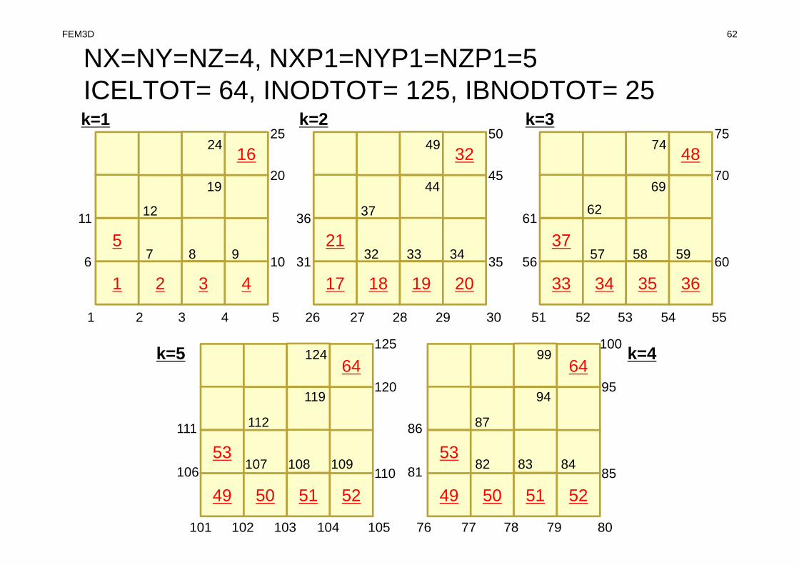
NX=NY=NZ=4, NXP1=NYP1=NZP1=5ICELTOT= 64, INODTOT= 125, IBNODTOT= 25
7 8 9
11 12
19
2425
20
k=1
32
21
17 18 19 20
2726 2928 30
31 3532 33 34
36 37
44
4950
45
k=2
48
37
33 34 35 36
5251 5453 55
56 6057 58 59
6162
69
7475
70
k=3
64
53
49 50 51 52
7776 7978 80
81 8582 83 84
86 87
94
99100
95
k=464
53
49 50 51 52
102101 104103 105
106 110107 108 109
111 112
119
124125
120
k=5

Example of “cube.0” Node Grp. Info.4 Number of Groups
25 50 75 100 Number of Nodes (ea. grp.)
Xmin1 6 11 16 21 26 31 36 41 46
51 56 61 66 71 76 81 86 91 96101 106 111 116 121
Ymin1 2 3 4 5 26 27 28 29 30
51 52 53 54 55 76 77 78 79 80101 102 103 104 105
Zmin1 2 3 4 5 6 7 8 9 10
11 12 13 14 15 16 17 18 19 2021 22 23 24 25
Zmax101 102 103 104 105 106 107 108 109 110111 112 113 114 115 116 117 118 119 120121 122 123 124 125
no use after this line
FEM3D 63
X
Y
Z
NYNX
NZ
T=0@Z=zmax

FEM3D 64
16
5
1 2 3 4
21 43 5
6 10
NX=NY=NZ=4, NXP1=NYP1=NZP1=5ICELTOT= 64, INODTOT= 125, IBNODTOT= 25
7 8 9
11 12
19
2425
20
k=1
32
21
17 18 19 20
2726 2928 30
31 3532 33 34
36 37
44
4950
45
k=2
48
37
33 34 35 36
5251 5453 55
56 6057 58 59
6162
69
7475
70
k=3
64
53
49 50 51 52
7776 7978 80
81 8582 83 84
86 87
94
99100
95
k=464
53
49 50 51 52
102101 104103 105
106 110107 108 109
111 112
119
124125
120
k=5
Xmin: i=1Ymin: j=1Zmin: k=1Zmax:k=5

Mesh Generation
• Big Technical & Research Issue– Complicated Geometry– Large Scale
• Parallelization is difficult
• Commercial Mesh Generator– FEMAP
• Interface to CAD Data Format
movie
FEM3D 65

• Formulation of 3D Element• 3D Heat Equations
– Galerkin Method– Element Matrices
• Running the Code• Data Structure• Overview of the Program
FEM3D 66

FEM Procedures: Program• Initialization
– Control Data– Node, Connectivity of Elements (N: Node#, NE: Elem#)– Initialization of Arrays (Global/Element Matrices)– Element-Global Matrix Mapping (Index, Item)
• Generation of Matrix– Element-by-Element Operations (do icel= 1, NE)
• Element matrices• Accumulation to global matrix
– Boundary Conditions
• Linear Solver– Conjugate Gradient Method
FEM3D 67

FEM3D 68
Structure of heat3D
test1main
input_cntlinput of control data
input_gridinput of mesh info
mat_con0connectivity of matrix
mat_con1connectivity of matrix
mat_ass_maincoefficient matrix
mat_ass_bcboundary conditions
solve11control of linear solver
output_ucdvisualization
mSORTsorting
jacobiJacobian
find_nodesearching nodes
cgCG solver
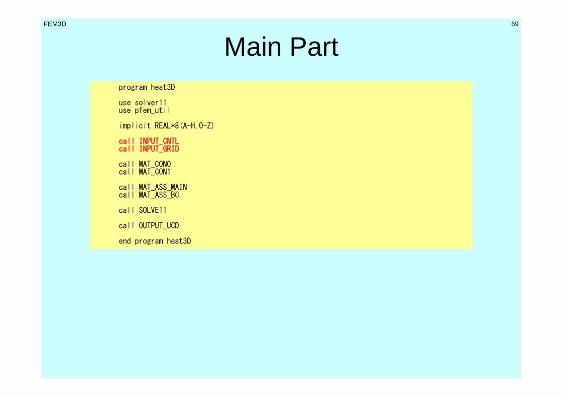
Main Partprogram heat3D
use solver11use pfem_util
implicit REAL*8(A-H,O-Z)
call INPUT_CNTLcall INPUT_GRID
call MAT_CON0call MAT_CON1
call MAT_ASS_MAINcall MAT_ASS_BC
call SOLVE11
call OUTPUT_UCD
end program heat3D
FEM3D 69
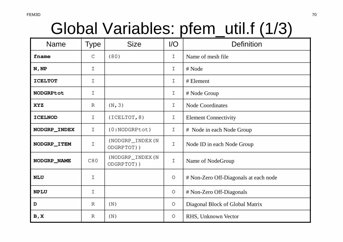
Global Variables: pfem_util.f (1/3) FEM3D 70
Name Type Size I/O Definition
fname C (80) I Name of mesh file
N,NP I I # Node
ICELTOT I I # Element
NODGRPtot I I # Node Group
XYZ R (N,3) I Node Coordinates
ICELNOD I (ICELTOT,8) I Element Connectivity
NODGRP_INDEX I (0:NODGRPtot) I # Node in each Node Group
NODGRP_ITEM I(NODGRP_INDEX(NODGRPTOT))
I Node ID in each Node Group
NODGRP_NAME C80(NODGRP_INDEX(NODGRPTOT))
I Name of NodeGroup
NLU I O # Non-Zero Off-Diagonals at each node
NPLU I O # Non-Zero Off-Diagonals
D R (N) O Diagonal Block of Global Matrix
B,X R (N) O RHS, Unknown Vector
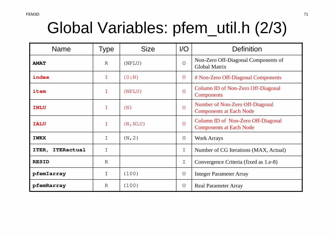
Global Variables: pfem_util.h (2/3) FEM3D 71
Name Type Size I/O Definition
AMAT R (NPLU) O Non-Zero Off-Diagonal Components of Global Matrix
index I (0:N) O # Non-Zero Off-Diagonal Components
item I (NPLU) O Column ID of Non-Zero Off-Diagonal Components
INLU I (N) O Number of Non-Zero Off-Diagonal Components at Each Node
IALU I (N,NLU) O Column ID of Non-Zero Off-Diagonal Components at Each Node
IWKX I (N,2) O Work Arrays
ITER, ITERactual I I Number of CG Iterations (MAX, Actual)
RESID R I Convergence Criteria (fixed as 1.e-8)
pfemIarray I (100) O Integer Parameter Array
pfemRarray R (100) O Real Parameter Array

Global Variables: pfem_util.h (3/3) FEM3D 72
Name Type Size I/O Definition
O8th R I = 0.125
PNQ, PNE, PNT R (2,2,8) O at each Gaussian Quad. Point
POS, WEI R (2) O Coordinates, Weighting Factor at each Gaussian Quad. Point
NCOL1, NCOL2 I (100) O Work arrays for sorting
SHAPE R (2,2,2,8) O Ni (i=1~8) at each Gaussian Quad Point
PNX, PNY, PNZ R (2,2,2,8) O at each Gaussian Quad. Point
DETJ R (2,2,2) O Determinant of Jacobian Matrix at each Gaussian Quad. Point
COND, QVOL R I Thermal Conductivity, Heat Generation Rate
( )8~1,, =∂∂
∂∂
∂∂
iNNN iii
ζηξ
( )8~1,, =∂
∂∂
∂∂
∂i
z
N
y
N
x
N iii
( ) 0,, =+
∂∂
∂∂+
∂∂
∂∂+
∂∂
∂∂
zyxQz
T
zy
T
yx
T
x&λλλ
( ) CC yxQVOLzyxQ +=,,&

INPUT_CNTL: Control Datasubroutine INPUT_CNTLuse pfem_util
implicit REAL*8 (A-H,O-Z)
open (11,file= 'INPUT.DAT', status='unknown')read (11,'(a80)') fnameread (11,*) ITERread (11,*) COND, QVOLread (11,*) RESIDclose (11)
pfemIarray(1)= ITERpfemRarray(1)= RESID
returnend
INPUT.DAT
cube.0 fname2000 ITER1.0 1.0 COND, QVOL1.0e-08 RESID
FEM3D 73

INPUT_GRID (1/3)!C***!C*** INPUT_GRID!C***!C
subroutine INPUT_GRIDuse pfem_utilimplicit REAL*8 (A-H,O-Z)
open (11, file= fname, status= 'unknown', form= 'formatted')
!C!C-- NODE
read (11,*) NNP= N
allocate (XYZ(N,3))XYZ= 0.d0
do i= 1, Nread (11,*) ii, (XYZ(i,kk),kk=1,3)
enddo
FEM3D 74
Example of “cube.0” Node125 = N
1 0.00 0.00 0.002 1.00 0.00 0.003 2.00 0.00 0.004 3.00 0.00 0.005 4.00 0.00 0.006 0.00 1.00 0.007 1.00 1.00 0.008 2.00 1.00 0.009 3.00 1.00 0.00
...
121 0.00 4.00 4.00122 1.00 4.00 4.00123 2.00 4.00 4.00124 3.00 4.00 4.00125 4.00 4.00 4.00
XYZ(i,3)
FEM3D 75
X
Y
Z
NYNX
NZ
T=0@Z=zmax
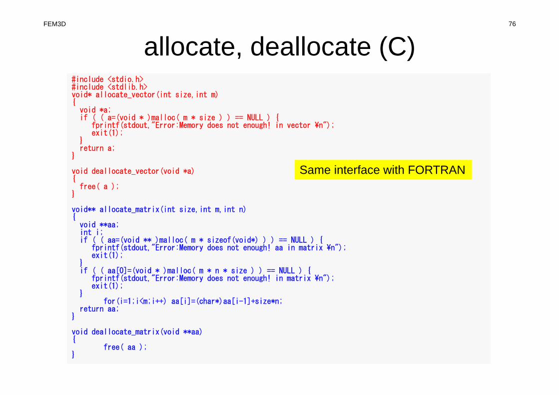
allocate, deallocate (C)#include <stdio.h>#include <stdlib.h>void* allocate_vector(int size,int m){
void *a;if ( ( a=(void * )malloc( m * size ) ) == NULL ) {
fprintf(stdout,"Error:Memory does not enough! in vector ¥n");exit(1);
}return a;
}
void deallocate_vector(void *a){
free( a );}
void** allocate_matrix(int size,int m,int n){
void **aa;int i;if ( ( aa=(void ** )malloc( m * sizeof(void*) ) ) == NULL ) {
fprintf(stdout,"Error:Memory does not enough! aa in matrix ¥n");exit(1);
}if ( ( aa[0]=(void * )malloc( m * n * size ) ) == NULL ) {
fprintf(stdout,"Error:Memory does not enough! in matrix ¥n");exit(1);
}for(i=1;i<m;i++) aa[i]=(char*)aa[i-1]+size*n;
return aa;}
void deallocate_matrix(void **aa){
free( aa );}
FEM3D 76
Same interface with FORTRAN

INPUT_GRID (2/3)!C!C-- ELEMENT
read (11,*) ICELTOTallocate (ICELNOD(ICELTOT,8))read (11,'(10i10)') (NTYPE, i= 1, ICELTOT)
do icel= 1, ICELTOTread (11,'(10i10,2i5,8i8)') ii, IMAT, (ICELNOD(icel,k), k=1,8)
enddo
FEM3D 77
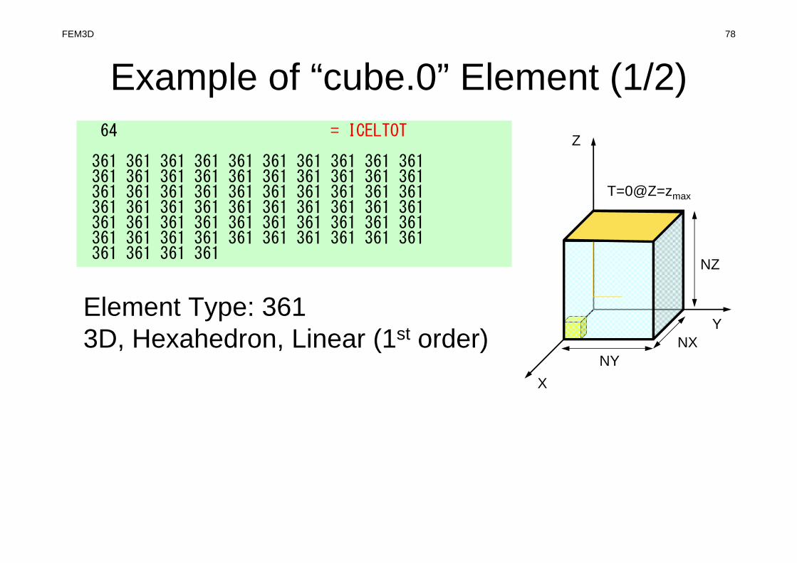
Example of “cube.0” Element (1/2)FEM3D 78
64 = ICELTOT
361 361 361 361 361 361 361 361 361 361361 361 361 361 361 361 361 361 361 361361 361 361 361 361 361 361 361 361 361361 361 361 361 361 361 361 361 361 361361 361 361 361 361 361 361 361 361 361361 361 361 361 361 361 361 361 361 361361 361 361 361
X
Y
Z
NYNX
NZ
T=0@Z=zmax
Element Type: 3613D, Hexahedron, Linear (1st order)

Example of “cube.0” Element (2/2)1 1 1 2 7 6 26 27 32 312 1 2 3 8 7 27 28 33 323 1 3 4 9 8 28 29 34 334 1 4 5 10 9 29 30 35 345 1 6 7 12 11 31 32 37 366 1 7 8 13 12 32 33 38 377 1 8 9 14 13 33 34 39 388 1 9 10 15 14 34 35 40 399 1 11 12 17 16 36 37 42 41
10 1 12 13 18 17 37 38 43 4211 1 13 14 19 18 38 39 44 4312 1 14 15 20 19 39 40 45 4413 1 16 17 22 21 41 42 47 46
...53 1 81 82 87 86 106 107 112 11154 1 82 83 88 87 107 108 113 11255 1 83 84 89 88 108 109 114 11356 1 84 85 90 89 109 110 115 11457 1 86 87 92 91 111 112 117 11658 1 87 88 93 92 112 113 118 11759 1 88 89 94 93 113 114 119 11860 1 89 90 95 94 114 115 120 11961 1 91 92 97 96 116 117 122 12162 1 92 93 98 97 117 118 123 12263 1 93 94 99 98 118 119 124 12364 1 94 95 100 99 119 120 125 124
iMAT ICELNOD(icel,8)
FEM3D 79
1 2
4 3
5 6
8 7
X
Y
Z
NYNX
NZ
T=0@Z=zmax
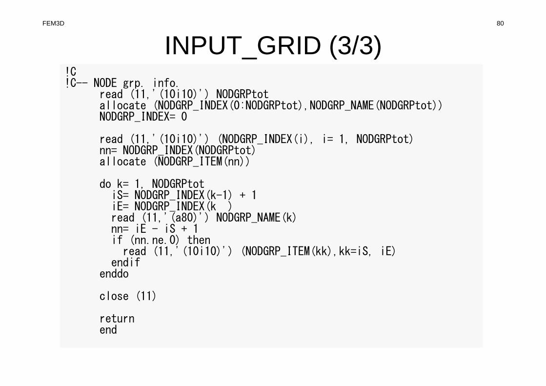
INPUT_GRID (3/3)!C!C-- NODE grp. info.
read (11,'(10i10)') NODGRPtotallocate (NODGRP_INDEX(0:NODGRPtot),NODGRP_NAME(NODGRPtot))NODGRP_INDEX= 0
read (11,'(10i10)') (NODGRP_INDEX(i), i= 1, NODGRPtot)nn= NODGRP_INDEX(NODGRPtot)allocate (NODGRP_ITEM(nn))
do k= 1, NODGRPtotiS= NODGRP_INDEX(k-1) + 1iE= NODGRP_INDEX(k )read (11,'(a80)') NODGRP_NAME(k)nn= iE - iS + 1if (nn.ne.0) then
read (11,'(10i10)') (NODGRP_ITEM(kk),kk=iS, iE)endif
enddo
close (11)
returnend
FEM3D 80
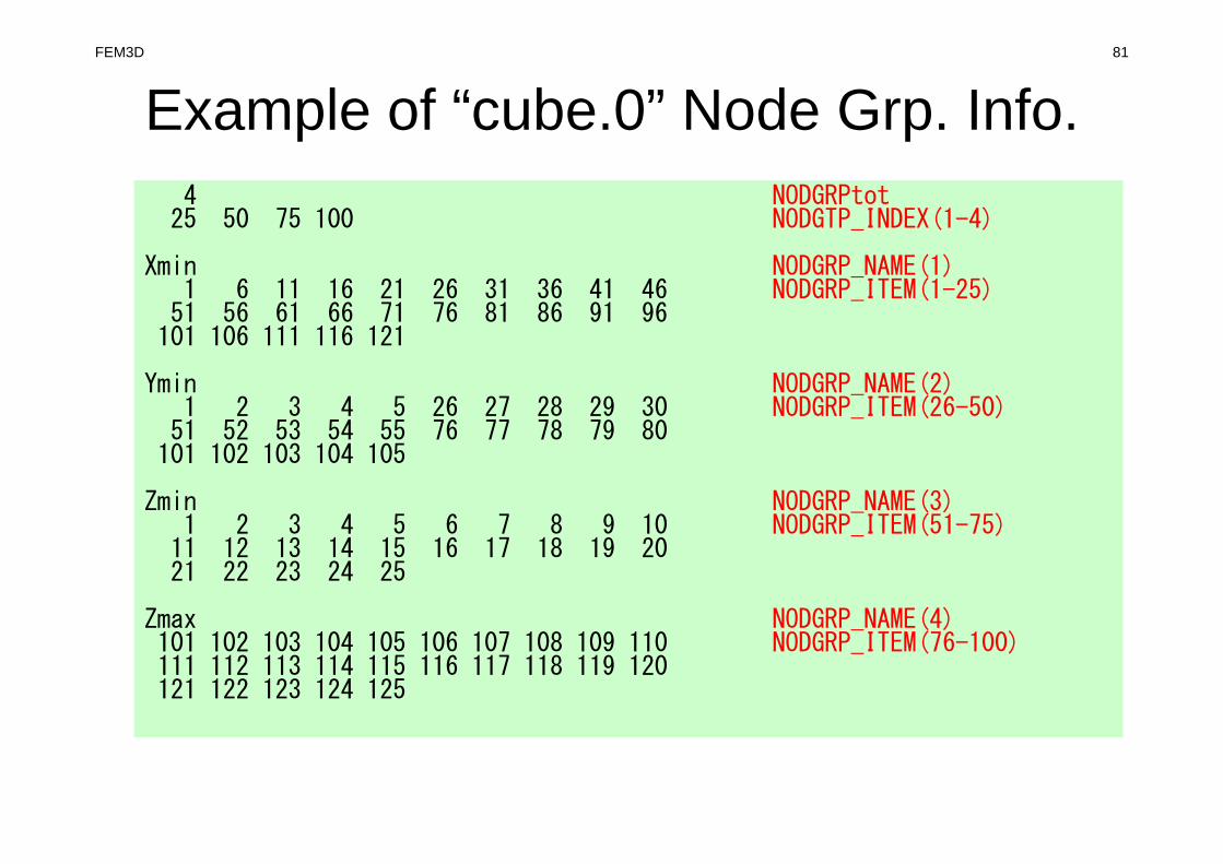
Example of “cube.0” Node Grp. Info.FEM3D 81
4 NODGRPtot25 50 75 100 NODGTP_INDEX(1-4)
Xmin NODGRP_NAME(1)1 6 11 16 21 26 31 36 41 46 NODGRP_ITEM(1-25)
51 56 61 66 71 76 81 86 91 96101 106 111 116 121
Ymin NODGRP_NAME(2)1 2 3 4 5 26 27 28 29 30 NODGRP_ITEM(26-50)
51 52 53 54 55 76 77 78 79 80101 102 103 104 105
Zmin NODGRP_NAME(3)1 2 3 4 5 6 7 8 9 10 NODGRP_ITEM(51-75)
11 12 13 14 15 16 17 18 19 2021 22 23 24 25
Zmax NODGRP_NAME(4)101 102 103 104 105 106 107 108 109 110 NODGRP_ITEM(76-100)111 112 113 114 115 116 117 118 119 120121 122 123 124 125

FEM3D 82
Structure of heat3D
test1main
input_cntlinput of control data
input_gridinput of mesh info
mat_con0connectivity of matrix
mat_con1connectivity of matrix
mat_ass_maincoefficient matrix
solve11control of linear solver
output_ucdvisualization
mSORTsorting
jacobiJacobian
find_nodesearching nodes
cgCG solver
mat_ass_bcboundary conditions

Global Variables: pfem_util.f (1/3) FEM3D 83
Name Type Size I/O Definition
fname C (80) I Name of mesh file
N,NP I I # Node
ICELTOT I I # Element
NODGRPtot I I # Node Group
XYZ R (N,3) I Node Coordinates
ICELNOD I (ICELTOT,8) I Element Connectivity
NODGRP_INDEX I (0:NODGRPtot) I # Node in each Node Group
NODGRP_ITEM I(NODGRP_INDEX(NODGRPTOT))
I Node ID in each Node Group
NODGRP_NAME C80(NODGRP_INDEX(NODGRPTOT))
I Name of NodeGroup
NLU I O # Non-Zero Off-Diagonals at each node
NPLU I O # Non-Zero Off-Diagonals
D R (N) O Diagonal Block of Global Matrix
B,X R (N) O RHS, Unknown Vector

Global Variables: pfem_util.f (2/3) FEM3D 84
Name Type Size I/O Definition
AMAT R (NPLU) O Non-Zero Off-Diagonal Components of Global Matrix
index I (0:N) O # Non-Zero Off-Diagonal Components
item I (NPLU) O Column ID of Non-Zero Off-Diagonal Components
INLU I (N) O Number of Non-Zero Off-Diagonal Components at Each Node
IALU I (N,NLU) O Column ID of Non-Zero Off-Diagonal Components at Each Node
IWKX I (N,2) O Work Arrays
ITER, ITERactual I I Number of CG Iterations (MAX, Actual)
RESID R I Convergence Criteria (fixed as 1.e-8)
pfemIarray I (100) O Integer Parameter Array
pfemRarray R (100) O Real Parameter Array

Global Variables: pfem_util.f (3/3) FEM3D 85
Name Type Size I/O Definition
O8th R I = 0.125
PNQ, PNE, PNT R (2,2,8) O at each Gaussian Quad. Point
POS, WEI R (2) O Coordinates, Weighting Factor at each Gaussian Quad. Point
NCOL1, NCOL2 I (100) O Work arrays for sorting
SHAPE R (2,2,2,8) O Ni (i=1~8) at each Gaussian Quad Point
PNX, PNY, PNZ R (2,2,2,8) O at each Gaussian Quad. Point
DETJ R (2,2,2) O Determinant of Jacobian Matrix at each Gaussian Quad. Point
COND, QVOL R I Thermal Conductivity, Heat Generation Rate
( )8~1,, =∂∂
∂∂
∂∂
iNNN iii
ζηξ
( )8~1,, =∂
∂∂
∂∂
∂i
z
N
y
N
x
N iii
( ) 0,, =+
∂∂
∂∂+
∂∂
∂∂+
∂∂
∂∂
zyxQz
T
zy
T
yx
T
x&λλλ
( ) CC yxQVOLzyxQ +=,,&

FEM3D 86
Towards Matrix Assembling• In 1D, it was easy to obtain information related to
indexand item.– 2 non-zero off-diagonals for each node– ID of non-zero off-diagonal : i+1, i-1, where “i” is node ID
• In 3D, situation is more complicated:– Number of non-zero off-diagonal components is between
7 and 26 for the current target problem– More complicated for real problems.– Generally, there are no information related to number of
non-zero off-diagonal components beforehand.
movie

FEM3D 87
Towards Matrix Assembling• In 1D, it was easy to obtain information related to
indexand item.– 2 non-zero off-diagonals for each node– ID of non-zero off-diagonal : i+1, i-1, where “i” is node ID
• In 3D, situation is more complicated:– Number of non-zero off-diagonal components is between
7 and 26 for the current target problem– More complicated for real problems.– Generally, there are no information related to number of
non-zero off-diagonal components beforehand.
• Count number of non-zero off-diagonals using arrays: INLU[N], IALU[N][NLU]

FEM3D 88
Main Partprogram heat3D
use solver11use pfem_util
implicit REAL*8(A-H,O-Z)
call INPUT_CNTLcall INPUT_GRID
call MAT_CON0call MAT_CON1
call MAT_ASS_MAINcall MAT_ASS_BC
call SOLVE11
call OUTPUT_UCD
end program heat3D
3
6
8
1
1
2
4 5
7 9
2 3 4
5 6 7 8
9 10 11 12
13 14 15 16
MAT_CON0: generates INU, IALUMAT_CON1: generates index, item
Node ID starting from “1”

FEM3D 89
MAT_CON0: Overview
do icel= 1, ICELTOTgenerate INLU, IALUaccording to 8 nodes of hex. elements(FIND_NODE)
enddo
( )1,1,1 −+−
( ) ( )1,1,1,, −−−=ζηξ1 2
34
5 6
78
( )1,1,1 −−+
( )1,1,1 −++
( )1,1,1 +−− ( )1,1,1 +−+
( )1,1,1 +++( )1,1,1 ++−
3
6
8
1
1
2
4 5
7 9
2 3 4
5 6 7 8
9 10 11 12
13 14 15 16
FEM3D 90
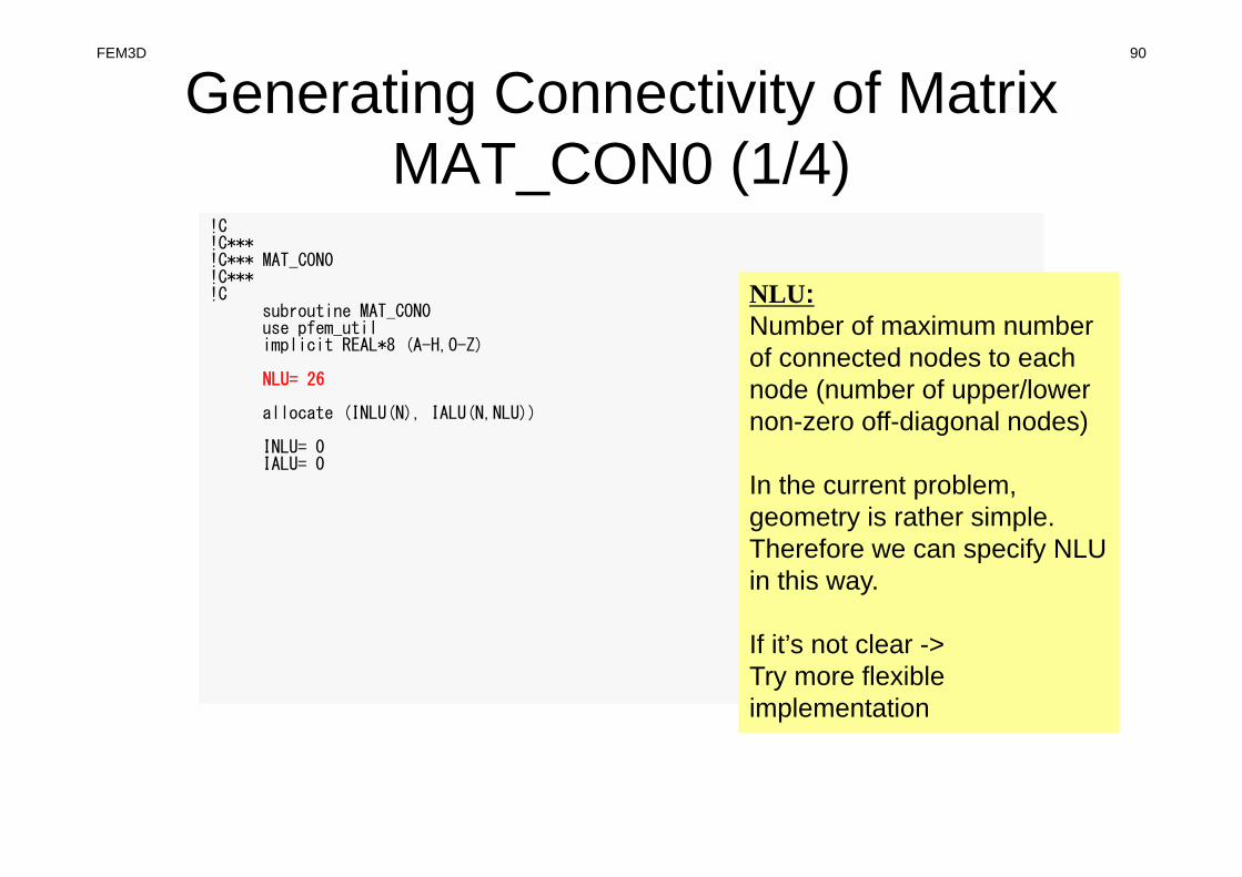
Generating Connectivity of MatrixMAT_CON0 (1/4)
!C!C***!C*** MAT_CON0!C***!C
subroutine MAT_CON0use pfem_utilimplicit REAL*8 (A-H,O-Z)
NLU= 26
allocate (INLU(N), IALU(N,NLU))
INLU= 0IALU= 0
NLU:Number of maximum number of connected nodes to each node (number of upper/lower non-zero off-diagonal nodes)
In the current problem, geometry is rather simple.Therefore we can specify NLU in this way.
If it’s not clear -> Try more flexible implementation

FEM3D 91
Generating Connectivity of MatrixMAT_CON0 (1/4)
!C!C***!C*** MAT_CON0!C***!C
subroutine MAT_CON0use pfem_utilimplicit REAL*8 (A-H,O-Z)
NLU= 26
allocate (INLU(N), IALU(N,NLU))
INLU= 0IALU= 0
Array Size Description
INLU (N)
Number of connected nodes to each node (lower/upper)
IALU (N,NLU)
Corresponding connected node ID (column ID)
FEM3D 92
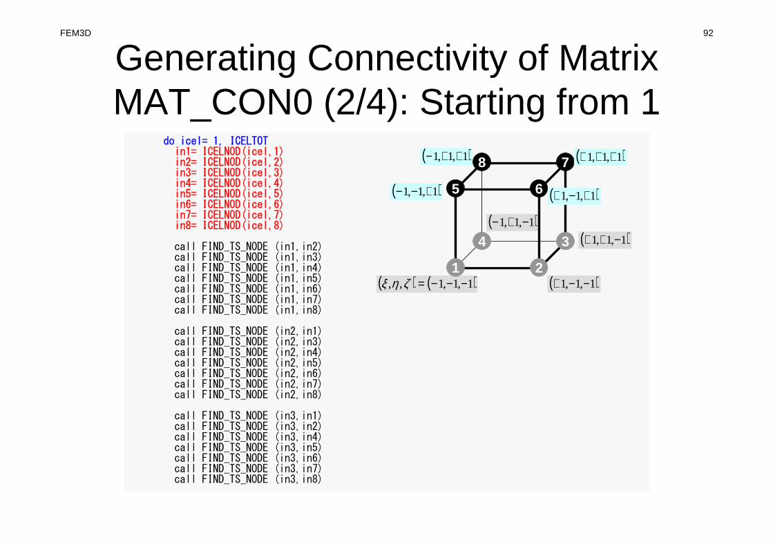
Generating Connectivity of MatrixMAT_CON0 (2/4): Starting from 1
do icel= 1, ICELTOTin1= ICELNOD(icel,1)in2= ICELNOD(icel,2)in3= ICELNOD(icel,3)in4= ICELNOD(icel,4)in5= ICELNOD(icel,5)in6= ICELNOD(icel,6)in7= ICELNOD(icel,7)in8= ICELNOD(icel,8)
call FIND_TS_NODE (in1,in2)call FIND_TS_NODE (in1,in3)call FIND_TS_NODE (in1,in4)call FIND_TS_NODE (in1,in5)call FIND_TS_NODE (in1,in6)call FIND_TS_NODE (in1,in7)call FIND_TS_NODE (in1,in8)
call FIND_TS_NODE (in2,in1)call FIND_TS_NODE (in2,in3)call FIND_TS_NODE (in2,in4)call FIND_TS_NODE (in2,in5)call FIND_TS_NODE (in2,in6)call FIND_TS_NODE (in2,in7)call FIND_TS_NODE (in2,in8)
call FIND_TS_NODE (in3,in1)call FIND_TS_NODE (in3,in2)call FIND_TS_NODE (in3,in4)call FIND_TS_NODE (in3,in5)call FIND_TS_NODE (in3,in6)call FIND_TS_NODE (in3,in7)call FIND_TS_NODE (in3,in8)
( )1,1,1 −+−
( ) ( )1,1,1,, −−−=ζηξ1 2
34
5 6
78
( )1,1,1 −−+
( )1,1,1 −++
( )1,1,1 +−− ( )1,1,1 +−+
( )1,1,1 +++( )1,1,1 ++−
FEM3D 93
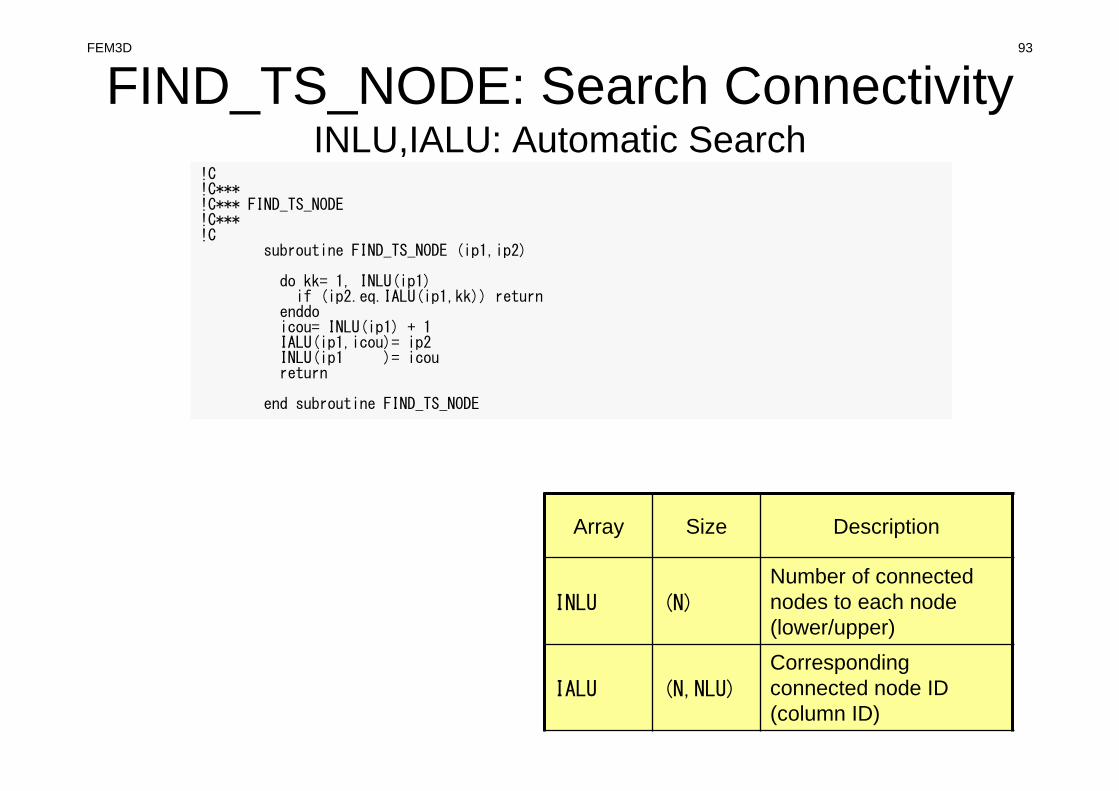
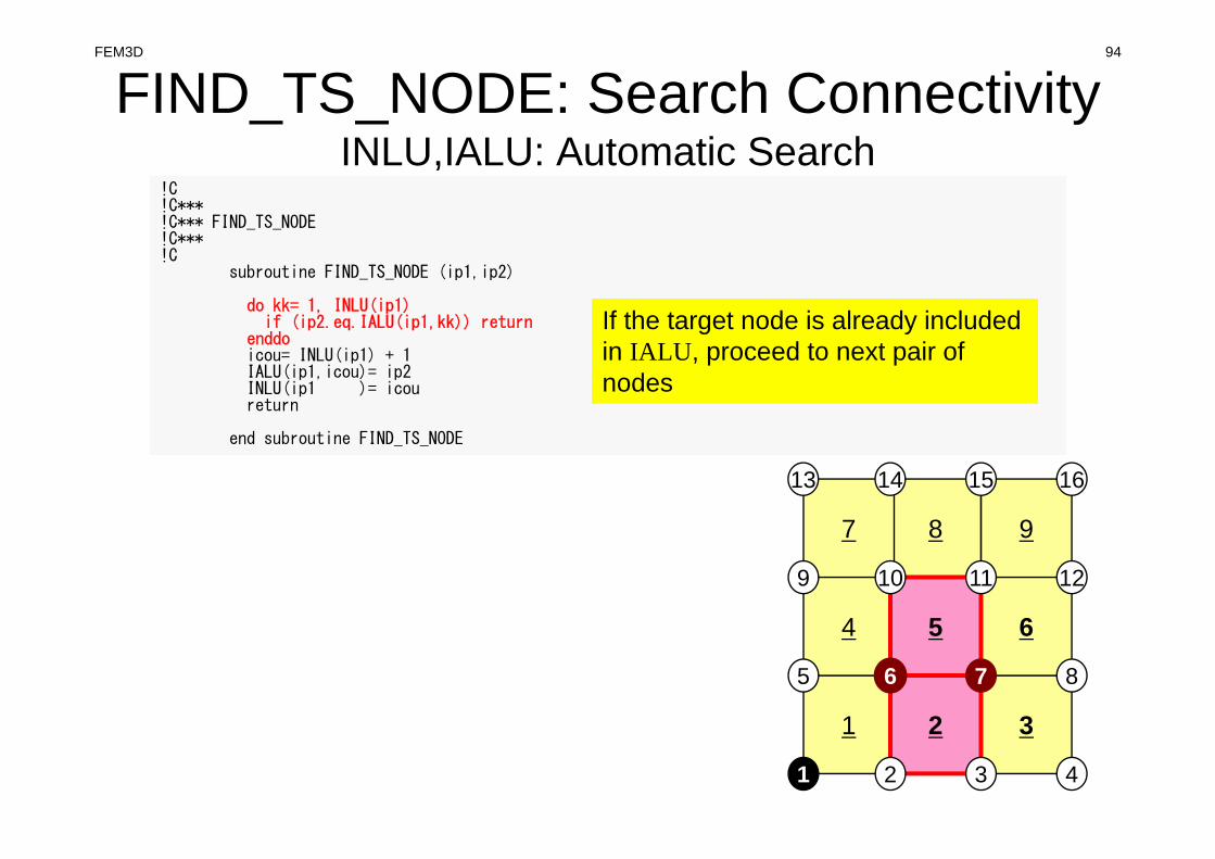
FIND_TS_NODE: Search ConnectivityINLU,IALU: Automatic Search
!C!C***!C*** FIND_TS_NODE!C***!C
subroutine FIND_TS_NODE (ip1,ip2)
do kk= 1, INLU(ip1)if (ip2.eq.IALU(ip1,kk)) return
enddoicou= INLU(ip1) + 1IALU(ip1,icou)= ip2INLU(ip1 )= icoureturn
end subroutine FIND_TS_NODE
Array Size Description
INLU (N)
Number of connected nodes to each node (lower/upper)
IALU (N,NLU)
Corresponding connected node ID (column ID)
!C!C***!C*** FIND_TS_NODE!C***!C
subroutine FIND_TS_NODE (ip1,ip2)
do kk= 1, INLU(ip1)if (ip2.eq.IALU(ip1,kk)) return
enddoicou= INLU(ip1) + 1IALU(ip1,icou)= ip2INLU(ip1 )= icoureturn
end subroutine FIND_TS_NODE
FEM3D 94
3
6
8
FIND_TS_NODE: Search ConnectivityINLU,IALU: Automatic Search
1
1
2
4 5
7 9
2 3 4
5 6 7 8
9 10 11 12
13 14 15 16
If the target node is already included in IALU , proceed to next pair of nodes

FEM3D 95
3
6
8
FIND_TS_NODE: Search ConnectivityINLU,IALU: Automatic Search
1
1
2
4 5
7 9
2 3 4
5 6 7 8
9 10 11 12
13 14 15 16
!C!C***!C*** FIND_TS_NODE!C***!C
subroutine FIND_TS_NODE (ip1,ip2)
do kk= 1, INLU(ip1)if (ip2.eq.IALU(ip1,kk)) return
enddoicou= INLU(ip1) + 1IALU(ip1,icou)= ip2INLU(ip1 )= icoureturn
end subroutine FIND_TS_NODE
If the target node is NOT included in IALU , store the node in IALU , and add 1 to INLU.

FEM3D 96
Generating Connectivity of MatrixMAT_CON0 (3/4)
call FIND_TS_NODE (in4,in1)call FIND_TS_NODE (in4,in2)call FIND_TS_NODE (in4,in3)call FIND_TS_NODE (in4,in5)call FIND_TS_NODE (in4,in6)call FIND_TS_NODE (in4,in7)call FIND_TS_NODE (in4,in8)
call FIND_TS_NODE (in5,in1)call FIND_TS_NODE (in5,in2)call FIND_TS_NODE (in5,in3)call FIND_TS_NODE (in5,in4)call FIND_TS_NODE (in5,in6)call FIND_TS_NODE (in5,in7)call FIND_TS_NODE (in5,in8)
call FIND_TS_NODE (in6,in1)call FIND_TS_NODE (in6,in2)call FIND_TS_NODE (in6,in3)call FIND_TS_NODE (in6,in4)call FIND_TS_NODE (in6,in5)call FIND_TS_NODE (in6,in7)call FIND_TS_NODE (in6,in8)
call FIND_TS_NODE (in7,in1)call FIND_TS_NODE (in7,in2)call FIND_TS_NODE (in7,in3)call FIND_TS_NODE (in7,in4)call FIND_TS_NODE (in7,in5)call FIND_TS_NODE (in7,in6)call FIND_TS_NODE (in7,in8)
( )1,1,1 −+−
( ) ( )1,1,1,, −−−=ζηξ1 2
34
5 6
78
( )1,1,1 −−+
( )1,1,1 −++
( )1,1,1 +−− ( )1,1,1 +−+
( )1,1,1 +++( )1,1,1 ++−

FEM3D 97
Generating Connectivity of MatrixMAT_CON0 (4/4)
call FIND_TS_NODE (in8,in1)call FIND_TS_NODE (in8,in2)call FIND_TS_NODE (in8,in3)call FIND_TS_NODE (in8,in4)call FIND_TS_NODE (in8,in5)call FIND_TS_NODE (in8,in6)call FIND_TS_NODE (in8,in7)
enddo
do in= 1, NNN= INLU(in)do k= 1, NNNCOL1(k)= IALU(in,k)
enddocall mSORT (NCOL1, NCOL2, NN)do k= NN, 1, -1IALU(in,NN-k+1)= NCOL1(NCOL2(k))
enddoenddo
Sort IALU(i,k) in ascending order by “bubble” sorting for less than 100 components.

FEM3D 98
MAT_CON1: CRS format!C!C***!C*** MAT_CON1!C***!C
subroutine MAT_CON1use pfem_utilimplicit REAL*8 (A-H,O-Z)
allocate (index(0:N))index= 0
do i= 1, Nindex(i)= index(i-1) + INLU(i)
enddo
NPLU= index(N)
allocate (item(NPLU))
do i= 1, Ndo k= 1, INLU(i)
kk = k + index(i-1)item(kk)= IALU(i,k)
enddoenddo
deallocate (INLU, IALU)
end subroutine MAT_CON1
0]0[index
][INLU]1[index
C
0
=
=+ ∑=
i
k
ki
00)(index
)(INLU)(index
FORTRAN
1
=
=∑=
i
k
ki

!C!C***!C*** MAT_CON1!C***!C
subroutine MAT_CON1use pfem_utilimplicit REAL*8 (A-H,O-Z)
allocate (index(0:N))index= 0
do i= 1, Nindex(i)= index(i-1) + INLU(i)
enddo
NPLU= index(N)
allocate (item(NPLU))
do i= 1, Ndo k= 1, INLU(i)
kk = k + index(i-1)item(kk)= IALU(i,k)
enddoenddo
deallocate (INLU, IALU)
end subroutine MAT_CON1
FEM3D 99
MAT_CON1: CRS format
NPLU=index(N)Size of array: itemTotal number of non-zero off-diagonal blocks

!C!C***!C*** MAT_CON1!C***!C
subroutine MAT_CON1use pfem_utilimplicit REAL*8 (A-H,O-Z)
allocate (index(0:N))index= 0
do i= 1, Nindex(i)= index(i-1) + INLU(i)
enddo
NPLU= index(N)
allocate (item(NPLU))
do i= 1, Ndo k= 1, INLU(i)
kk = k + index(i-1)item(kk)= IALU(i,k)
enddoenddo
deallocate (INLU, IALU)
end subroutine MAT_CON1
FEM3D 100
MAT_CON1: CRS format
itemstore node ID starting from 1

!C!C***!C*** MAT_CON1!C***!C
subroutine MAT_CON1use pfem_utilimplicit REAL*8 (A-H,O-Z)
allocate (index(0:N))index= 0
do i= 1, Nindex(i)= index(i-1) + INLU(i)
enddo
NPLU= index(N)
allocate (item(NPLU))
do i= 1, Ndo k= 1, INLU(i)
kk = k + index(i-1)item(kk)= IALU(i,k)
enddoenddo
deallocate (INLU, IALU)
end subroutine MAT_CON1
FEM3D 101
MAT_CON1: CRS format
Not required any more
FEM3D 102
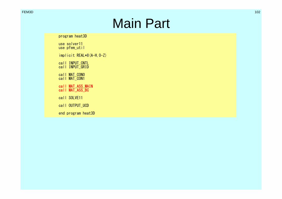
Main Partprogram heat3D
use solver11use pfem_util
implicit REAL*8(A-H,O-Z)
call INPUT_CNTLcall INPUT_GRID
call MAT_CON0call MAT_CON1
call MAT_ASS_MAINcall MAT_ASS_BC
call SOLVE11
call OUTPUT_UCD
end program heat3D

FEM3D 103
MAT_ASS_MAIN: Overviewdo kpn= 1, 2 Gaussian Quad. points in ζ-direction
do jpn= 1, 2 Gaussian Quad. points in η-directiondo ipn= 1, 2 Gaussian Quad. Pointe in ξ-direction
Define Shape Function at Gaussian Quad. Points (8-points)Its derivative on natural/local coordinate is also defined.
enddoenddo
enddo
do icel= 1, ICELTOT Loop for Element
Jacobian and derivative on global coordinate of shape functions at Gaussian Quad. Points are defined according to coordinates of 8 nodes.(JACOBI)
do ie= 1, 8 Local Node ID
do je= 1, 8 Local Node IDGlobal Node ID: ip, jpAddress of Aip,jp in “item”: kk
do kpn= 1, 2 Gaussian Quad. points in ζ-directiondo jpn= 1, 2 Gaussian Quad. points in η-direction
do ipn= 1, 2 Gaussian Quad. points in ξ-directionintegration on each elementcoefficients of element matricesaccumulation to global matrix
enddoenddo
enddoenddo
enddoenddo
ie
je

FEM3D 104
MAT_ASS_MAIN (1/6)!C!C***!C*** MAT_ASS_MAIN!C***!C
subroutine MAT_ASS_MAINuse pfem_utilimplicit REAL*8 (A-H,O-Z)integer(kind=kint), dimension( 8) :: nodLOCAL
allocate (AMAT(NPLU))allocate (B(N), D(N), X(N))
AMAT= 0.d0 Non-Zero Off-Diagonal components (coef. matrix)B= 0.d0 RHS vectorX= 0.d0 UnknownsD= 0.d0 Diagonal components (coef. matrix)
WEI(1)= +1.0000000000D+00WEI(2)= +1.0000000000D+00
POS(1)= -0.5773502692D+00POS(2)= +0.5773502692D+00

FEM3D 105
MAT_ASS_MAIN (1/6)!C!C***!C*** MAT_ASS_MAIN!C***!C
subroutine MAT_ASS_MAINuse pfem_utilimplicit REAL*8 (A-H,O-Z)integer(kind=kint), dimension( 8) :: nodLOCAL
allocate (AMAT(NPLU))allocate (B(N), D(N), X(N))
AMAT= 0.d0B= 0.d0X= 0.d0D= 0.d0
WEI(1)= +1.0000000000D+00WEI(2)= +1.0000000000D+00
POS(1)= -0.5773502692D+00POS(2)= +0.5773502692D+00
POS: Quad. PointWEI: Weighting Factor

FEM3D 106
MAT_ASS_MAIN (2/6)!C!C-- INIT.!C PNQ - 1st-order derivative of shape function by QSI!C PNE - 1st-order derivative of shape function by ETA!C PNT - 1st-order derivative of shape function by ZET!C
do kp= 1, 2do jp= 1, 2do ip= 1, 2
QP1= 1.d0 + POS(ip)QM1= 1.d0 - POS(ip)EP1= 1.d0 + POS(jp)EM1= 1.d0 - POS(jp)TP1= 1.d0 + POS(kp)TM1= 1.d0 - POS(kp)
SHAPE(ip,jp,kp,1)= O8th * QM1 * EM1 * TM1SHAPE(ip,jp,kp,2)= O8th * QP1 * EM1 * TM1SHAPE(ip,jp,kp,3)= O8th * QP1 * EP1 * TM1SHAPE(ip,jp,kp,4)= O8th * QM1 * EP1 * TM1SHAPE(ip,jp,kp,5)= O8th * QM1 * EM1 * TP1SHAPE(ip,jp,kp,6)= O8th * QP1 * EM1 * TP1SHAPE(ip,jp,kp,7)= O8th * QP1 * EP1 * TP1SHAPE(ip,jp,kp,8)= O8th * QM1 * EP1 * TP1
FEM3D 107
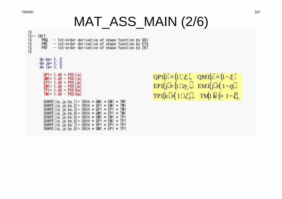
MAT_ASS_MAIN (2/6)!C!C-- INIT.!C PNQ - 1st-order derivative of shape function by QSI!C PNE - 1st-order derivative of shape function by ETA!C PNT - 1st-order derivative of shape function by ZET!C
do kp= 1, 2do jp= 1, 2do ip= 1, 2
QP1= 1.d0 + POS(ip)QM1= 1.d0 - POS(ip)EP1= 1.d0 + POS(jp)EM1= 1.d0 - POS(jp)TP1= 1.d0 + POS(kp)TM1= 1.d0 - POS(kp)
SHAPE(ip,jp,kp,1)= O8th * QM1 * EM1 * TM1SHAPE(ip,jp,kp,2)= O8th * QP1 * EM1 * TM1SHAPE(ip,jp,kp,3)= O8th * QP1 * EP1 * TM1SHAPE(ip,jp,kp,4)= O8th * QM1 * EP1 * TM1SHAPE(ip,jp,kp,5)= O8th * QM1 * EM1 * TP1SHAPE(ip,jp,kp,6)= O8th * QP1 * EM1 * TP1SHAPE(ip,jp,kp,7)= O8th * QP1 * EP1 * TP1SHAPE(ip,jp,kp,8)= O8th * QM1 * EP1 * TP1
( ) ( ) ( ) ( )( ) ( ) ( ) ( )( ) ( ) ( ) ( )kk
ij
ii
ζζηηξξ
−=+=
−=+=−=+=
1kTM1,1kTP1
1jEM1,1jEP1
1iQM1,1iQP1
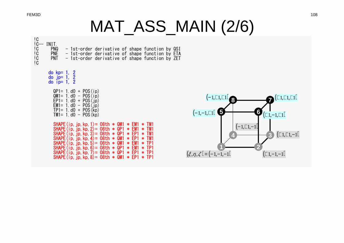
FEM3D 108
MAT_ASS_MAIN (2/6)!C!C-- INIT.!C PNQ - 1st-order derivative of shape function by QSI!C PNE - 1st-order derivative of shape function by ETA!C PNT - 1st-order derivative of shape function by ZET!C
do kp= 1, 2do jp= 1, 2do ip= 1, 2
QP1= 1.d0 + POS(ip)QM1= 1.d0 - POS(ip)EP1= 1.d0 + POS(jp)EM1= 1.d0 - POS(jp)TP1= 1.d0 + POS(kp)TM1= 1.d0 - POS(kp)
SHAPE(ip,jp,kp,1)= O8th * QM1 * EM1 * TM1SHAPE(ip,jp,kp,2)= O8th * QP1 * EM1 * TM1SHAPE(ip,jp,kp,3)= O8th * QP1 * EP1 * TM1SHAPE(ip,jp,kp,4)= O8th * QM1 * EP1 * TM1SHAPE(ip,jp,kp,5)= O8th * QM1 * EM1 * TP1SHAPE(ip,jp,kp,6)= O8th * QP1 * EM1 * TP1SHAPE(ip,jp,kp,7)= O8th * QP1 * EP1 * TP1SHAPE(ip,jp,kp,8)= O8th * QM1 * EP1 * TP1
( )1,1,1 −+−
( ) ( )1,1,1,, −−−=ζηξ1 2
34
5 6
78
( )1,1,1 −−+
( )1,1,1 −++
( )1,1,1 +−− ( )1,1,1 +−+
( )1,1,1 +++( )1,1,1 ++−
FEM3D 109
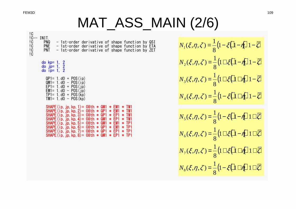
MAT_ASS_MAIN (2/6)!C!C-- INIT.!C PNQ - 1st-order derivative of shape function by QSI!C PNE - 1st-order derivative of shape function by ETA!C PNT - 1st-order derivative of shape function by ZET!C
do kp= 1, 2do jp= 1, 2do ip= 1, 2
QP1= 1.d0 + POS(ip)QM1= 1.d0 - POS(ip)EP1= 1.d0 + POS(jp)EM1= 1.d0 - POS(jp)TP1= 1.d0 + POS(kp)TM1= 1.d0 - POS(kp)
SHAPE(ip,jp,kp,1)= O8th * QM1 * EM1 * TM1SHAPE(ip,jp,kp,2)= O8th * QP1 * EM1 * TM1SHAPE(ip,jp,kp,3)= O8th * QP1 * EP1 * TM1SHAPE(ip,jp,kp,4)= O8th * QM1 * EP1 * TM1SHAPE(ip,jp,kp,5)= O8th * QM1 * EM1 * TP1SHAPE(ip,jp,kp,6)= O8th * QP1 * EM1 * TP1SHAPE(ip,jp,kp,7)= O8th * QP1 * EP1 * TP1SHAPE(ip,jp,kp,8)= O8th * QM1 * EP1 * TP1
( )( )( )
( )( )( )
( )( )( )
( )( )( )ζηξζηξ
ζηξζηξ
ζηξζηξ
ζηξζηξ
−+−=
−++=
−−+=
−−−=
1118
1),,(
1118
1),,(
1118
1),,(
1118
1),,(
4
3
2
1
N
N
N
N
( )( )( )
( )( )( )
( )( )( )
( )( )( )ζηξζηξ
ζηξζηξ
ζηξζηξ
ζηξζηξ
++−=
+++=
+−+=
+−−=
1118
1),,(
1118
1),,(
1118
1),,(
1118
1),,(
8
7
6
5
N
N
N
N

FEM3D 110
MAT_ASS_MAIN (3/6)PNQ(jp,kp,1)= - O8th * EM1 * TM1PNQ(jp,kp,2)= + O8th * EM1 * TM1PNQ(jp,kp,3)= + O8th * EP1 * TM1PNQ(jp,kp,4)= - O8th * EP1 * TM1PNQ(jp,kp,5)= - O8th * EM1 * TP1PNQ(jp,kp,6)= + O8th * EM1 * TP1PNQ(jp,kp,7)= + O8th * EP1 * TP1PNQ(jp,kp,8)= - O8th * EP1 * TP1PNE(ip,kp,1)= - O8th * QM1 * TM1PNE(ip,kp,2)= - O8th * QP1 * TM1PNE(ip,kp,3)= + O8th * QP1 * TM1PNE(ip,kp,4)= + O8th * QM1 * TM1PNE(ip,kp,5)= - O8th * QM1 * TP1PNE(ip,kp,6)= - O8th * QP1 * TP1PNE(ip,kp,7)= + O8th * QP1 * TP1PNE(ip,kp,8)= + O8th * QM1 * TP1PNT(ip,jp,1)= - O8th * QM1 * EM1PNT(ip,jp,2)= - O8th * QP1 * EM1PNT(ip,jp,3)= - O8th * QP1 * EP1PNT(ip,jp,4)= - O8th * QM1 * EP1PNT(ip,jp,5)= + O8th * QM1 * EM1PNT(ip,jp,6)= + O8th * QP1 * EM1PNT(ip,jp,7)= + O8th * QP1 * EP1PNT(ip,jp,8)= + O8th * QM1 * EP1
enddoenddoenddo
do icel= 1, ICELTOTCOND0= COND
in1= ICELNOD(icel,1)in2= ICELNOD(icel,2)in3= ICELNOD(icel,3)in4= ICELNOD(icel,4)in5= ICELNOD(icel,5)in6= ICELNOD(icel,6)in7= ICELNOD(icel,7)in8= ICELNOD(icel,8)
),,(),( kjilN
kjPNQ ζζηηξξξ
===∂∂=
( )( )
( )( )
( )( )
( )( )kjkji
kjkji
kjkji
kjkji
N
N
N
N
ζηζηξξ
ζηζηξξ
ζηζηξξ
ζηζηξξ
−+−=∂∂
−++=∂∂
−−+=∂
∂
−−−=∂∂
118
1),,(
118
1),,(
118
1),,(
118
1),,(
3
3
2
1
),,(),( kjilN
kiPNE ζζηηξξη
===∂∂=
),,(),( kjilN
jiPNT ζζηηξξζ
===∂∂=
),,( kji ζηξ
First Order Derivative of Shape Functions at

FEM3D 111
MAT_ASS_MAIN (3/6)PNQ(jp,kp,1)= - O8th * EM1 * TM1PNQ(jp,kp,2)= + O8th * EM1 * TM1PNQ(jp,kp,3)= + O8th * EP1 * TM1PNQ(jp,kp,4)= - O8th * EP1 * TM1PNQ(jp,kp,5)= - O8th * EM1 * TP1PNQ(jp,kp,6)= + O8th * EM1 * TP1PNQ(jp,kp,7)= + O8th * EP1 * TP1PNQ(jp,kp,8)= - O8th * EP1 * TP1PNE(ip,kp,1)= - O8th * QM1 * TM1PNE(ip,kp,2)= - O8th * QP1 * TM1PNE(ip,kp,3)= + O8th * QP1 * TM1PNE(ip,kp,4)= + O8th * QM1 * TM1PNE(ip,kp,5)= - O8th * QM1 * TP1PNE(ip,kp,6)= - O8th * QP1 * TP1PNE(ip,kp,7)= + O8th * QP1 * TP1PNE(ip,kp,8)= + O8th * QM1 * TP1PNT(ip,jp,1)= - O8th * QM1 * EM1PNT(ip,jp,2)= - O8th * QP1 * EM1PNT(ip,jp,3)= - O8th * QP1 * EP1PNT(ip,jp,4)= - O8th * QM1 * EP1PNT(ip,jp,5)= + O8th * QM1 * EM1PNT(ip,jp,6)= + O8th * QP1 * EM1PNT(ip,jp,7)= + O8th * QP1 * EP1PNT(ip,jp,8)= + O8th * QM1 * EP1
enddoenddoenddo
do icel= 1, ICELTOTCOND0= COND
in1= ICELNOD(icel,1)in2= ICELNOD(icel,2)in3= ICELNOD(icel,3)in4= ICELNOD(icel,4)in5= ICELNOD(icel,5)in6= ICELNOD(icel,6)in7= ICELNOD(icel,7)in8= ICELNOD(icel,8)
( )1,1,1 −+−
( ) ( )1,1,1,, −−−=ζηξ1 2
34
5 6
78
( )1,1,1 −−+
( )1,1,1 −++
( )1,1,1 +−− ( )1,1,1 +−+
( )1,1,1 +++( )1,1,1 ++−

FEM3D 112
MAT_ASS_MAIN (4/6)nodLOCAL(1)= in1nodLOCAL(2)= in2nodLOCAL(3)= in3nodLOCAL(4)= in4nodLOCAL(5)= in5nodLOCAL(6)= in6nodLOCAL(7)= in7nodLOCAL(8)= in8
X1= XYZ(in1,1)X2= XYZ(in2,1)X3= XYZ(in3,1)X4= XYZ(in4,1)X5= XYZ(in5,1)X6= XYZ(in6,1)X7= XYZ(in7,1)X8= XYZ(in8,1)Y1= XYZ(in1,2)Y2= XYZ(in2,2)Y3= XYZ(in3,2)Y4= XYZ(in4,2)Y5= XYZ(in5,2)Y6= XYZ(in6,2)Y7= XYZ(in7,2)Y8= XYZ(in8,2)QVC= O8th * (X1+X2+X3+X4+X5+X6+X7+X8+
& Y1+Y2+Y3+Y4+Y5+Y6+Y7+Y8)Z1= XYZ(in1,3)Z2= XYZ(in2,3)Z3= XYZ(in3,3)Z4= XYZ(in4,3)Z5= XYZ(in5,3)Z6= XYZ(in6,3)Z7= XYZ(in7,3)Z8= XYZ(in8,3)
call JACOBI (DETJ, PNQ, PNE, PNT, PNX, PNY, PNZ, && X1, X2, X3, X4, X5, X6, X7, X8, && Y1, Y2, Y3, Y4, Y5, Y6, Y7, Y8, && Z1, Z2, Z3, Z4, Z5, Z6, Z7, Z8 )
( )1,1,1 −+−
( ) ( )1,1,1,, −−−=ζηξ1 2
34
5 6
78
( )1,1,1 −−+
( )1,1,1 −++
( )1,1,1 +−− ( )1,1,1 +−+
( )1,1,1 +++( )1,1,1 ++−Node ID (Global)

FEM3D 113
MAT_ASS_MAIN (4/6)nodLOCAL(1)= in1nodLOCAL(2)= in2nodLOCAL(3)= in3nodLOCAL(4)= in4nodLOCAL(5)= in5nodLOCAL(6)= in6nodLOCAL(7)= in7nodLOCAL(8)= in8
X1= XYZ(in1,1)X2= XYZ(in2,1)X3= XYZ(in3,1)X4= XYZ(in4,1)X5= XYZ(in5,1)X6= XYZ(in6,1)X7= XYZ(in7,1)X8= XYZ(in8,1)Y1= XYZ(in1,2)Y2= XYZ(in2,2)Y3= XYZ(in3,2)Y4= XYZ(in4,2)Y5= XYZ(in5,2)Y6= XYZ(in6,2)Y7= XYZ(in7,2)Y8= XYZ(in8,2)QVC= O8th * (X1+X2+X3+X4+X5+X6+X7+X8+
& Y1+Y2+Y3+Y4+Y5+Y6+Y7+Y8)Z1= XYZ(in1,3)Z2= XYZ(in2,3)Z3= XYZ(in3,3)Z4= XYZ(in4,3)Z5= XYZ(in5,3)Z6= XYZ(in6,3)Z7= XYZ(in7,3)Z8= XYZ(in8,3)
call JACOBI (DETJ, PNQ, PNE, PNT, PNX, PNY, PNZ, && X1, X2, X3, X4, X5, X6, X7, X8, && Y1, Y2, Y3, Y4, Y5, Y6, Y7, Y8, && Z1, Z2, Z3, Z4, Z5, Z6, Z7, Z8 )
( )1,1,1 −+−
( ) ( )1,1,1,, −−−=ζηξ1 2
34
5 6
78
( )1,1,1 −−+
( )1,1,1 −++
( )1,1,1 +−− ( )1,1,1 +−+
( )1,1,1 +++( )1,1,1 ++−
X-Coordinatesof 8 nodes
Y-Coordinatesof 8 nodes
Z-Coordinatesof 8 nodes

FEM3D 114
MAT_ASS_MAIN (4/6)nodLOCAL(1)= in1nodLOCAL(2)= in2nodLOCAL(3)= in3nodLOCAL(4)= in4nodLOCAL(5)= in5nodLOCAL(6)= in6nodLOCAL(7)= in7nodLOCAL(8)= in8
X1= XYZ(in1,1)X2= XYZ(in2,1)X3= XYZ(in3,1)X4= XYZ(in4,1)X5= XYZ(in5,1)X6= XYZ(in6,1)X7= XYZ(in7,1)X8= XYZ(in8,1)Y1= XYZ(in1,2)Y2= XYZ(in2,2)Y3= XYZ(in3,2)Y4= XYZ(in4,2)Y5= XYZ(in5,2)Y6= XYZ(in6,2)Y7= XYZ(in7,2)Y8= XYZ(in8,2)QVC= O8th * (X1+X2+X3+X4+X5+X6+X7+X8+
& Y1+Y2+Y3+Y4+Y5+Y6+Y7+Y8)Z1= XYZ(in1,3)Z2= XYZ(in2,3)Z3= XYZ(in3,3)Z4= XYZ(in4,3)Z5= XYZ(in5,3)Z6= XYZ(in6,3)Z7= XYZ(in7,3)Z8= XYZ(in8,3)
call JACOBI (DETJ, PNQ, PNE, PNT, PNX, PNY, PNZ, && X1, X2, X3, X4, X5, X6, X7, X8, && Y1, Y2, Y3, Y4, Y5, Y6, Y7, Y8, && Z1, Z2, Z3, Z4, Z5, Z6, Z7, Z8 )
( )1,1,1 −+−
( ) ( )1,1,1,, −−−=ζηξ1 2
34
5 6
78
( )1,1,1 −−+
( )1,1,1 −++
( )1,1,1 +−− ( )1,1,1 +−+
( )1,1,1 +++( )1,1,1 ++−
( ) 0,, =+
∂∂
∂∂+
∂∂
∂∂+
∂∂
∂∂
zyxQz
T
zy
T
yx
T
x&λλλ
( ) CC yxQVOLzyxQ +=,,&
Heat Gen. Rate is a function of location (cell center: xc,yc)
X-Coordinatesof 8 nodes
Y-Coordinatesof 8 nodes
FEM3D 115
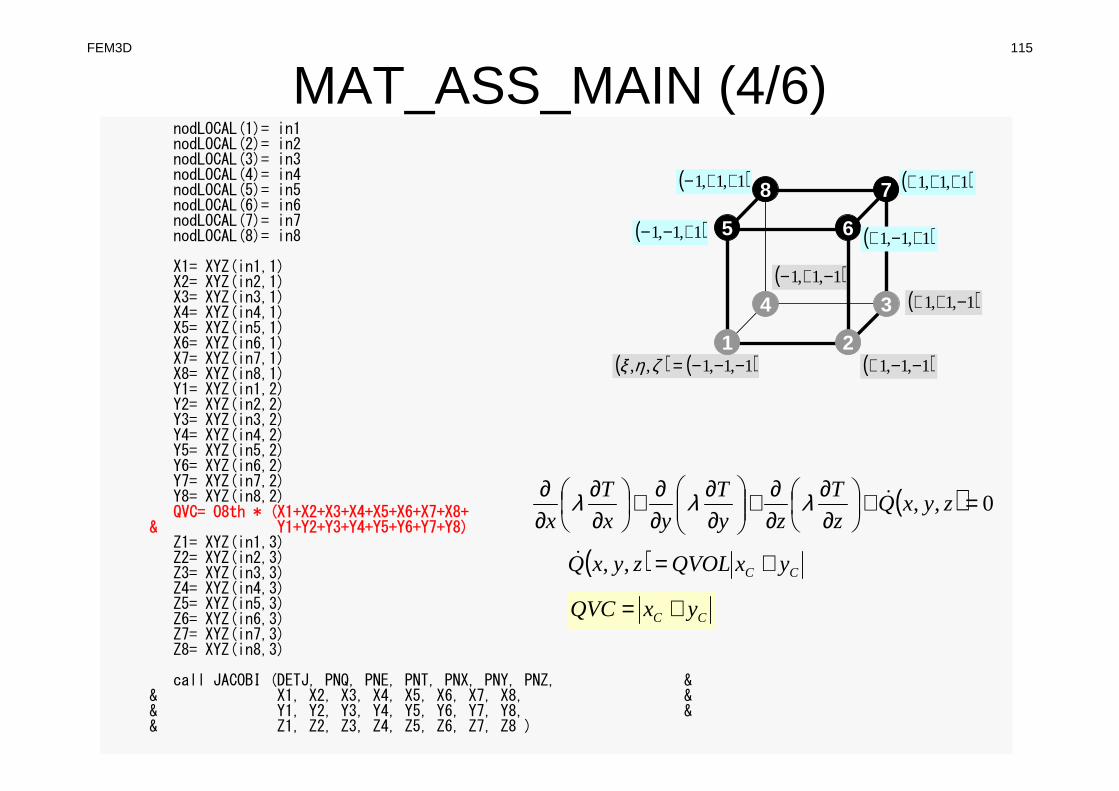
MAT_ASS_MAIN (4/6)nodLOCAL(1)= in1nodLOCAL(2)= in2nodLOCAL(3)= in3nodLOCAL(4)= in4nodLOCAL(5)= in5nodLOCAL(6)= in6nodLOCAL(7)= in7nodLOCAL(8)= in8
X1= XYZ(in1,1)X2= XYZ(in2,1)X3= XYZ(in3,1)X4= XYZ(in4,1)X5= XYZ(in5,1)X6= XYZ(in6,1)X7= XYZ(in7,1)X8= XYZ(in8,1)Y1= XYZ(in1,2)Y2= XYZ(in2,2)Y3= XYZ(in3,2)Y4= XYZ(in4,2)Y5= XYZ(in5,2)Y6= XYZ(in6,2)Y7= XYZ(in7,2)Y8= XYZ(in8,2)QVC= O8th * (X1+X2+X3+X4+X5+X6+X7+X8+
& Y1+Y2+Y3+Y4+Y5+Y6+Y7+Y8)Z1= XYZ(in1,3)Z2= XYZ(in2,3)Z3= XYZ(in3,3)Z4= XYZ(in4,3)Z5= XYZ(in5,3)Z6= XYZ(in6,3)Z7= XYZ(in7,3)Z8= XYZ(in8,3)
call JACOBI (DETJ, PNQ, PNE, PNT, PNX, PNY, PNZ, && X1, X2, X3, X4, X5, X6, X7, X8, && Y1, Y2, Y3, Y4, Y5, Y6, Y7, Y8, && Z1, Z2, Z3, Z4, Z5, Z6, Z7, Z8 )
( )1,1,1 −+−
( ) ( )1,1,1,, −−−=ζηξ1 2
34
5 6
78
( )1,1,1 −−+
( )1,1,1 −++
( )1,1,1 +−− ( )1,1,1 +−+
( )1,1,1 +++( )1,1,1 ++−
( ) 0,, =+
∂∂
∂∂+
∂∂
∂∂+
∂∂
∂∂
zyxQz
T
zy
T
yx
T
x&λλλ
( ) CC yxQVOLzyxQ +=,,&
CC yxQVC +=
FEM3D 116
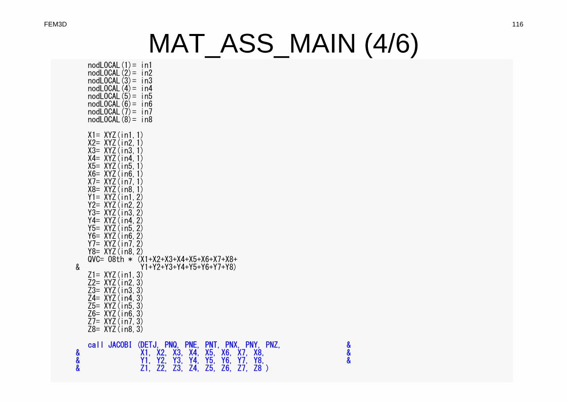
MAT_ASS_MAIN (4/6)nodLOCAL(1)= in1nodLOCAL(2)= in2nodLOCAL(3)= in3nodLOCAL(4)= in4nodLOCAL(5)= in5nodLOCAL(6)= in6nodLOCAL(7)= in7nodLOCAL(8)= in8
X1= XYZ(in1,1)X2= XYZ(in2,1)X3= XYZ(in3,1)X4= XYZ(in4,1)X5= XYZ(in5,1)X6= XYZ(in6,1)X7= XYZ(in7,1)X8= XYZ(in8,1)Y1= XYZ(in1,2)Y2= XYZ(in2,2)Y3= XYZ(in3,2)Y4= XYZ(in4,2)Y5= XYZ(in5,2)Y6= XYZ(in6,2)Y7= XYZ(in7,2)Y8= XYZ(in8,2)QVC= O8th * (X1+X2+X3+X4+X5+X6+X7+X8+
& Y1+Y2+Y3+Y4+Y5+Y6+Y7+Y8)Z1= XYZ(in1,3)Z2= XYZ(in2,3)Z3= XYZ(in3,3)Z4= XYZ(in4,3)Z5= XYZ(in5,3)Z6= XYZ(in6,3)Z7= XYZ(in7,3)Z8= XYZ(in8,3)
call JACOBI (DETJ, PNQ, PNE, PNT, PNX, PNY, PNZ, && X1, X2, X3, X4, X5, X6, X7, X8, && Y1, Y2, Y3, Y4, Y5, Y6, Y7, Y8, && Z1, Z2, Z3, Z4, Z5, Z6, Z7, Z8 )

FEM3D 117
JACOBI (1/4)subroutine JACOBI (DETJ, PNQ, PNE, PNT, PNX, PNY, PNZ, && X1, X2, X3, X4, X5, X6, X7, X8, Y1, Y2, Y3, Y4, Y5, Y6, Y7, Y8, && Z1, Z2, Z3, Z4, Z5, Z6, Z7, Z8 )
!C!C calculates JACOBIAN & INVERSE JACOBIAN!C dNi/dx, dNi/dy & dNi/dz!C
implicit REAL*8 (A-H,O-Z)dimension DETJ(2,2,2)dimension PNQ(2,2,8), PNE(2,2,8), PNT(2,2,8)dimension PNX(2,2,2,8), PNY(2,2,2,8), PNZ(2,2,2,8)
do kp= 1, 2do jp= 1, 2do ip= 1, 2
PNX(ip,jp,kp,1)=0.d0PNX(ip,jp,kp,2)=0.d0PNX(ip,jp,kp,3)=0.d0PNX(ip,jp,kp,4)=0.d0PNX(ip,jp,kp,5)=0.d0PNX(ip,jp,kp,6)=0.d0PNX(ip,jp,kp,7)=0.d0PNX(ip,jp,kp,8)=0.d0PNY(ip,jp,kp,1)=0.d0PNY(ip,jp,kp,2)=0.d0PNY(ip,jp,kp,3)=0.d0PNY(ip,jp,kp,4)=0.d0PNY(ip,jp,kp,5)=0.d0PNY(ip,jp,kp,6)=0.d0PNY(ip,jp,kp,7)=0.d0PNY(ip,jp,kp,8)=0.d0PNZ(ip,jp,kp,1)=0.d0PNZ(ip,jp,kp,2)=0.d0PNZ(ip,jp,kp,3)=0.d0PNZ(ip,jp,kp,4)=0.d0PNZ(ip,jp,kp,5)=0.d0PNZ(ip,jp,kp,6)=0.d0PNZ(ip,jp,kp,7)=0.d0PNZ(ip,jp,kp,8)=0.d0
Input ( ) ( )8~1,,,,, =
∂∂
∂∂
∂∂
lzyxNNN
llllll
ζηξ
Jz
N
y
N
x
N lll det,,,
∂∂
∂∂
∂∂
Output
Values at each Gaussian Quad. Points: (ip,jp,kp)

FEM3D 118
Partial Diff. on Natural Coord. (1/4)
• According to formulae:
ζζζζζηξ
ηηηηζηξ
ξξξξζηξ
∂∂
∂∂+
∂∂
∂∂+
∂∂
∂∂=
∂∂
∂∂
∂∂+
∂∂
∂∂+
∂∂
∂∂=
∂∂
∂∂
∂∂+
∂∂
∂∂+
∂∂
∂∂=
∂∂
z
z
Ny
y
Nx
x
NN
z
z
Ny
y
Nx
x
NN
z
z
Ny
y
Nx
x
NN
iiii
iiii
iiii
),,(
),,(
),,(
∂∂
∂∂
∂∂
ζηξiii NNN
,,
∂∂
∂∂
∂∂
z
N
y
N
x
N iii ,,
can be easily derived according to definitions.
are required for computations.
FEM3D 119
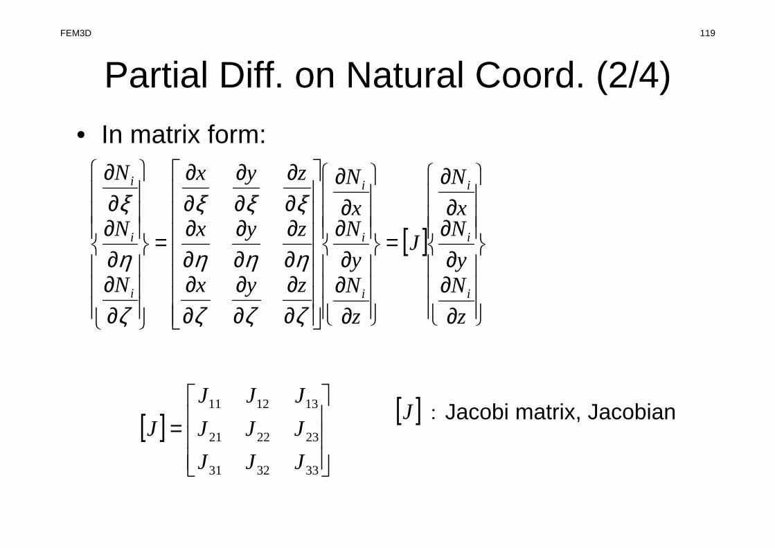
Partial Diff. on Natural Coord. (2/4)
• In matrix form:
[ ]
∂∂∂
∂∂
∂
=
∂∂∂
∂∂
∂
∂∂
∂∂
∂∂
∂∂
∂∂
∂∂
∂∂
∂∂
∂∂
=
∂∂∂∂∂∂
z
Ny
Nx
N
J
z
Ny
Nx
N
zyx
zyx
zyx
N
N
N
i
i
i
i
i
i
i
i
i
ζζζ
ηηη
ξξξ
ζ
η
ξ
[ ]
=
333231
232221
131211
JJJ
JJJ
JJJ
J[ ]J : Jacobi matrix, Jacobian
FEM3D 120
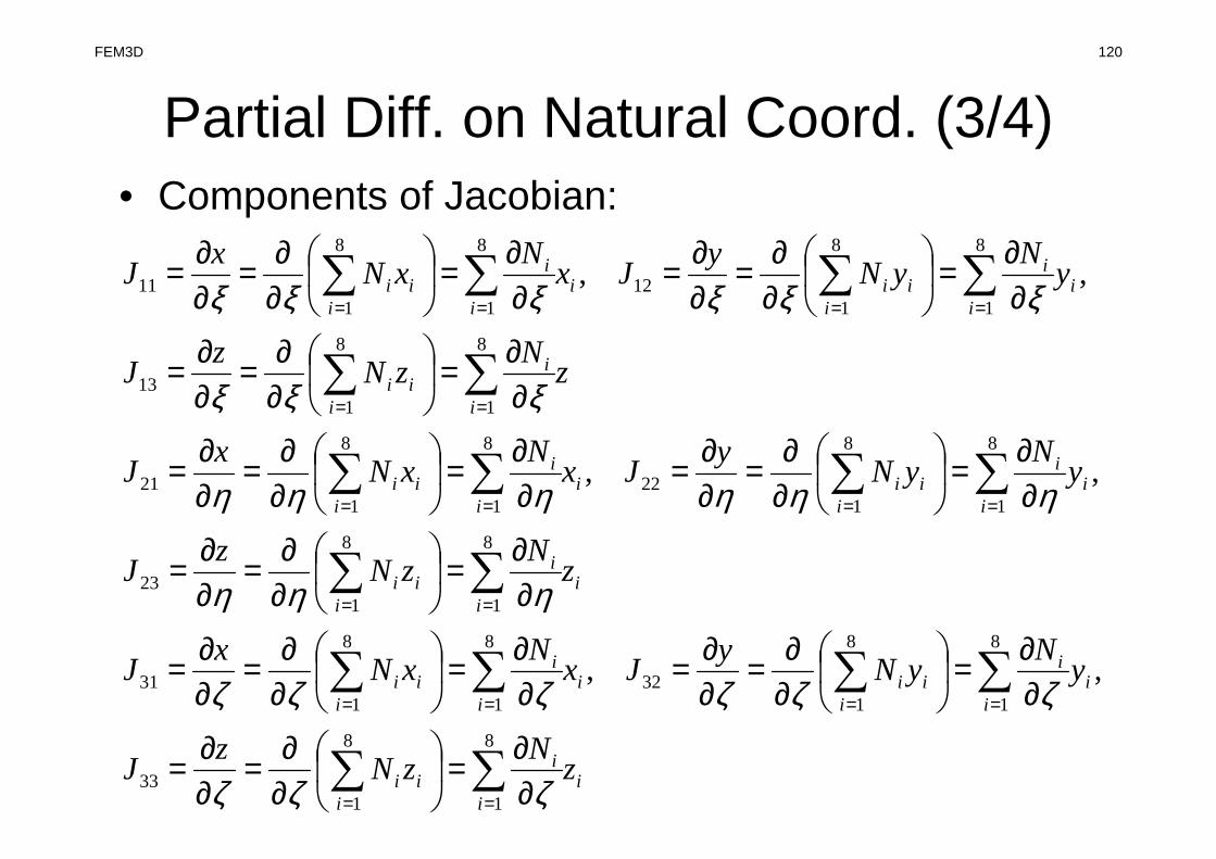
Partial Diff. on Natural Coord. (3/4)• Components of Jacobian:
ii
ii
ii
ii
ii
iii
i
ii
ii
ii
ii
ii
ii
ii
iii
i
ii
ii
i
ii
ii
ii
ii
iii
i
ii
ii
zN
zNz
J
yN
yNy
JxN
xNx
J
zN
zNz
J
yN
yNy
JxN
xNx
J
zN
zNz
J
yN
yNy
JxN
xNx
J
∑∑
∑∑∑∑
∑∑
∑∑∑∑
∑∑
∑∑∑∑
==
====
==
====
==
====
∂∂=
∂∂=
∂∂=
∂∂=
∂∂=
∂∂=
∂∂=
∂∂=
∂∂=
∂∂=
∂∂=
∂∂=
∂∂=
∂∂=
∂∂=
∂∂=
∂∂=
∂∂=
∂∂=
∂∂=
∂∂=
∂∂=
∂∂=
∂∂=
∂∂=
∂∂=
∂∂=
8
1
8
133
8
1
8
132
8
1
8
131
8
1
8
123
8
1
8
122
8
1
8
121
8
1
8
113
8
1
8
112
8
1
8
111
,,
,,
,,
ζζζ
ζζζζζζ
ηηη
ηηηηηη
ξξξ
ξξξξξξ

FEM3D 121
JACOBI (2/4)!C!C== DETERMINANT of the JACOBIAN
dXdQ = && + PNQ(jp,kp,1) * X1 + PNQ(jp,kp,2) * X2 && + PNQ(jp,kp,3) * X3 + PNQ(jp,kp,4) * X4 && + PNQ(jp,kp,5) * X5 + PNQ(jp,kp,6) * X6 && + PNQ(jp,kp,7) * X7 + PNQ(jp,kp,8) * X8
dYdQ = && + PNQ(jp,kp,1) * Y1 + PNQ(jp,kp,2) * Y2 && + PNQ(jp,kp,3) * Y3 + PNQ(jp,kp,4) * Y4 && + PNQ(jp,kp,5) * Y5 + PNQ(jp,kp,6) * Y6 && + PNQ(jp,kp,7) * Y7 + PNQ(jp,kp,8) * Y8
dZdQ = && + PNQ(jp,kp,1) * Z1 + PNQ(jp,kp,2) * Z2 && + PNQ(jp,kp,3) * Z3 + PNQ(jp,kp,4) * Z4 && + PNQ(jp,kp,5) * Z5 + PNQ(jp,kp,6) * Z6 && + PNQ(jp,kp,7) * Z7 + PNQ(jp,kp,8) * Z8
dXdE = && + PNE(ip,kp,1) * X1 + PNE(ip,kp,2) * X2 && + PNE(ip,kp,3) * X3 + PNE(ip,kp,4) * X4 && + PNE(ip,kp,5) * X5 + PNE(ip,kp,6) * X6 && + PNE(ip,kp,7) * X7 + PNE(ip,kp,8) * X8
dYdE = && + PNE(ip,kp,1) * Y1 + PNE(ip,kp,2) * Y2 && + PNE(ip,kp,3) * Y3 + PNE(ip,kp,4) * Y4 && + PNE(ip,kp,5) * Y5 + PNE(ip,kp,6) * Y6 && + PNE(ip,kp,7) * Y7 + PNE(ip,kp,8) * Y8
dZdE = && + PNE(ip,kp,1) * Z1 + PNE(ip,kp,2) * Z2 && + PNE(ip,kp,3) * Z3 + PNE(ip,kp,4) * Z4 && + PNE(ip,kp,5) * Z5 + PNE(ip,kp,6) * Z6 && + PNE(ip,kp,7) * Z7 + PNE(ip,kp,8) * Z8 13
12
11
dZdQ
dYdQ
dXdQ
Jz
Jy
Jx
=∂∂=
=∂∂=
=∂∂=
ξ
ξ
ξ
[ ]
=
333231
232221
131211
JJJ
JJJ
JJJ
J

FEM3D 122
JACOBI (3/4)dXdT = &
& + PNT(ip,jp,1) * X1 + PNT(ip,jp,2) * X2 && + PNT(ip,jp,3) * X3 + PNT(ip,jp,4) * X4 && + PNT(ip,jp,5) * X5 + PNT(ip,jp,6) * X6 && + PNT(ip,jp,7) * X7 + PNT(ip,jp,8) * X8
dYdT = && + PNT(ip,jp,1) * Y1 + PNT(ip,jp,2) * Y2 && + PNT(ip,jp,3) * Y3 + PNT(ip,jp,4) * Y4 && + PNT(ip,jp,5) * Y5 + PNT(ip,jp,6) * Y6 && + PNT(ip,jp,7) * Y7 + PNT(ip,jp,8) * Y8
dZdT = && + PNT(ip,jp,1) * Z1 + PNT(ip,jp,2) * Z2 && + PNT(ip,jp,3) * Z3 + PNT(ip,jp,4) * Z4 && + PNT(ip,jp,5) * Z5 + PNT(ip,jp,6) * Z6 && + PNT(ip,jp,7) * Z7 + PNT(ip,jp,8) * Z8
DETJ(ip,jp,kp)= dXdQ*(dYdE*dZdT-dZdE*dYdT) + && dYdQ*(dZdE*dXdT-dXdE*dZdT) + && dZdQ*(dXdE*dYdT-dYdE*dXdT)
!C!C== INVERSE JACOBIAN
coef= 1.d0 / DETJ(ip,jp,kp)
a11= coef * ( dYdE*dZdT - dZdE*dYdT )a12= coef * ( dZdQ*dYdT - dYdQ*dZdT )a13= coef * ( dYdQ*dZdE - dZdQ*dYdE )
a21= coef * ( dZdE*dXdT - dXdE*dZdT )a22= coef * ( dXdQ*dZdT - dZdQ*dXdT )a23= coef * ( dZdQ*dXdE - dXdQ*dZdE )
a31= coef * ( dXdE*dYdT - dYdE*dXdT )a32= coef * ( dYdQ*dXdT - dXdQ*dYdT )a33= coef * ( dXdQ*dYdE - dYdQ*dXdE )
DETJ(ip,jp,kp)= dabs(DETJ(ip,jp,kp))
[ ]
=
333231
232221
131211
JJJ
JJJ
JJJ
J

FEM3D 123
Partial Diff. on Natural Coord. (4/4)
• Partial differentiation on global coordinate system is introduced as follows (with inverse of Jacobian matrix (3×3))
[ ]
∂∂∂∂∂∂
=
∂∂∂∂∂∂
∂∂
∂∂
∂∂
∂∂
∂∂
∂∂
∂∂
∂∂
∂∂
=
∂∂∂
∂∂
∂
−
−
ζ
η
ξ
ζ
η
ξ
ζζζ
ηηη
ξξξ
i
i
i
i
i
i
i
i
i
N
N
N
J
N
N
N
zyx
zyx
zyx
z
Ny
Nx
N
1
1

FEM3D 124
JACOBI (3/4)dXdT = &
& + PNT(ip,jp,1) * X1 + PNT(ip,jp,2) * X2 && + PNT(ip,jp,3) * X3 + PNT(ip,jp,4) * X4 && + PNT(ip,jp,5) * X5 + PNT(ip,jp,6) * X6 && + PNT(ip,jp,7) * X7 + PNT(ip,jp,8) * X8
dYdT = && + PNT(ip,jp,1) * Y1 + PNT(ip,jp,2) * Y2 && + PNT(ip,jp,3) * Y3 + PNT(ip,jp,4) * Y4 && + PNT(ip,jp,5) * Y5 + PNT(ip,jp,6) * Y6 && + PNT(ip,jp,7) * Y7 + PNT(ip,jp,8) * Y8
dZdT = && + PNT(ip,jp,1) * Z1 + PNT(ip,jp,2) * Z2 && + PNT(ip,jp,3) * Z3 + PNT(ip,jp,4) * Z4 && + PNT(ip,jp,5) * Z5 + PNT(ip,jp,6) * Z6 && + PNT(ip,jp,7) * Z7 + PNT(ip,jp,8) * Z8
DETJ(ip,jp,kp)= dXdQ*(dYdE*dZdT-dZdE*dYdT) + && dYdQ*(dZdE*dXdT-dXdE*dZdT) + && dZdQ*(dXdE*dYdT-dYdE*dXdT)
!C!C== INVERSE JACOBIAN
coef= 1.d0 / DETJ(ip,jp,kp)
a11= coef * ( dYdE*dZdT - dZdE*dYdT )a12= coef * ( dZdQ*dYdT - dYdQ*dZdT )a13= coef * ( dYdQ*dZdE - dZdQ*dYdE )
a21= coef * ( dZdE*dXdT - dXdE*dZdT )a22= coef * ( dXdQ*dZdT - dZdQ*dXdT )a23= coef * ( dZdQ*dXdE - dXdQ*dZdE )
a31= coef * ( dXdE*dYdT - dYdE*dXdT )a32= coef * ( dYdQ*dXdT - dXdQ*dYdT )a33= coef * ( dXdQ*dYdE - dYdQ*dXdE )
DETJ(ip,jp,kp)= dabs(DETJ(ip,jp,kp))
[ ]
=−
333231
232221
1312111
aaa
aaa
aaa
J

FEM3D 125
JACOBI (4/4)!C!C== set the dNi/dX, dNi/dY & dNi/dZ components
PNX(ip,jp,kp,1)= a11*PNQ(jp,kp,1) + a12*PNE(ip,kp,1) + a13*PNT(ip,jp,1)PNX(ip,jp,kp,2)= a11*PNQ(jp,kp,2) + a12*PNE(ip,kp,2) + a13*PNT(ip,jp,2)PNX(ip,jp,kp,3)= a11*PNQ(jp,kp,3) + a12*PNE(ip,kp,3) + a13*PNT(ip,jp,3)PNX(ip,jp,kp,4)= a11*PNQ(jp,kp,4) + a12*PNE(ip,kp,4) + a13*PNT(ip,jp,4)PNX(ip,jp,kp,5)= a11*PNQ(jp,kp,5) + a12*PNE(ip,kp,5) + a13*PNT(ip,jp,5)PNX(ip,jp,kp,6)= a11*PNQ(jp,kp,6) + a12*PNE(ip,kp,6) + a13*PNT(ip,jp,6)PNX(ip,jp,kp,7)= a11*PNQ(jp,kp,7) + a12*PNE(ip,kp,7) + a13*PNT(ip,jp,7)PNX(ip,jp,kp,8)= a11*PNQ(jp,kp,8) + a12*PNE(ip,kp,8) + a13*PNT(ip,jp,8)
PNY(ip,jp,kp,1)= a21*PNQ(jp,kp,1) + a22*PNE(ip,kp,1) + a23*PNT(ip,jp,1)PNY(ip,jp,kp,2)= a21*PNQ(jp,kp,2) + a22*PNE(ip,kp,2) + a23*PNT(ip,jp,2)PNY(ip,jp,kp,3)= a21*PNQ(jp,kp,3) + a22*PNE(ip,kp,3) + a23*PNT(ip,jp,3)PNY(ip,jp,kp,4)= a21*PNQ(jp,kp,4) + a22*PNE(ip,kp,4) + a23*PNT(ip,jp,4)PNY(ip,jp,kp,5)= a21*PNQ(jp,kp,5) + a22*PNE(ip,kp,5) + a23*PNT(ip,jp,5)PNY(ip,jp,kp,6)= a21*PNQ(jp,kp,6) + a22*PNE(ip,kp,6) + a23*PNT(ip,jp,6)PNY(ip,jp,kp,7)= a21*PNQ(jp,kp,7) + a22*PNE(ip,kp,7) + a23*PNT(ip,jp,7)PNY(ip,jp,kp,8)= a21*PNQ(jp,kp,8) + a22*PNE(ip,kp,8) + a23*PNT(ip,jp,8)
PNZ(ip,jp,kp,1)= a31*PNQ(jp,kp,1) + a32*PNE(ip,kp,1) + a33*PNT(ip,jp,1)PNZ(ip,jp,kp,2)= a31*PNQ(jp,kp,2) + a32*PNE(ip,kp,2) + a33*PNT(ip,jp,2)PNZ(ip,jp,kp,3)= a31*PNQ(jp,kp,3) + a32*PNE(ip,kp,3) + a33*PNT(ip,jp,3)PNZ(ip,jp,kp,4)= a31*PNQ(jp,kp,4) + a32*PNE(ip,kp,4) + a33*PNT(ip,jp,4)PNZ(ip,jp,kp,5)= a31*PNQ(jp,kp,5) + a32*PNE(ip,kp,5) + a33*PNT(ip,jp,5)PNZ(ip,jp,kp,6)= a31*PNQ(jp,kp,6) + a32*PNE(ip,kp,6) + a33*PNT(ip,jp,6)PNZ(ip,jp,kp,7)= a31*PNQ(jp,kp,7) + a32*PNE(ip,kp,7) + a33*PNT(ip,jp,7)PNZ(ip,jp,kp,8)= a31*PNQ(jp,kp,8) + a32*PNE(ip,kp,8) + a33*PNT(ip,jp,8)
enddoenddoenddo
∂∂∂∂∂∂
=
∂∂∂∂∂∂
∂∂
∂∂
∂∂
∂∂
∂∂
∂∂
∂∂
∂∂
∂∂
=
∂∂∂
∂∂
∂−
ζ
η
ξ
ζ
η
ξ
ζζζ
ηηη
ξξξ
i
i
i
i
i
i
i
i
i
N
N
N
aaa
aaa
aaa
N
N
N
zyx
zyx
zyx
z
Ny
Nx
N
333231
232221
131211
1

FEM3D 126
MAT_ASS_MAIN (5/6)!C!C== CONSTRUCT the GLOBAL MATRIX
do ie= 1, 8ip = nodLOCAL(ie)
do je= 1, 8jp = nodLOCAL(je)
kk= 0if (jp.ne.ip) theniiS= index(ip-1) + 1iiE= index(ip )do k= iiS, iiE
if ( item(k).eq.jp ) thenkk= kexit
endifenddo
endif
( )1,1,1 −+−
( ) ( )1,1,1,, −−−=ζηξ1 2
34
5 6
78
( )1,1,1 −−+
( )1,1,1 −++
( )1,1,1 +−− ( )1,1,1 +−+
( )1,1,1 +++( )1,1,1 ++−
Non-Zero Off-Diagonal Blockin Global Matix
jpipA ,
kk: address in “item”
ip= nodLOCAL[ie]jp= nodLOCAL[je]
Node ID (ip,jp)starting from 1

Element Matrix: 8x8
( )1,1,1 −+−
( ) ( )1,1,1,, −−−=ζηξ1 2
34
5 6
78
( )1,1,1 −−+
( )1,1,1 −++
( )1,1,1 +−− ( )1,1,1 +−+
( )1,1,1 +++( )1,1,1 ++−
i
j
[ ] ( )81, K=jikij
FEM3D 127

FEM3D 128
MAT_ASS_MAIN (5/6)!C!C== CONSTRUCT the GLOBAL MATRIX
do ie= 1, 8ip = nodLOCAL(ie)
do je= 1, 8jp = nodLOCAL(je)
kk= 0if (jp.ne.ip) theniiS= index(ip-1) + 1iiE= index(ip )do k= iiS, iiE
if ( item(k).eq.jp ) thenkk= kexit
endifenddo
endif
( )1,1,1 −+−
( ) ( )1,1,1,, −−−=ζηξ1 2
34
5 6
78
( )1,1,1 −−+
( )1,1,1 −++
( )1,1,1 +−− ( )1,1,1 +−+
( )1,1,1 +++( )1,1,1 ++−
Element Matrix(ie~je): Local IDGlobal Matrix (ip~jp): Global ID
kk:address in “item” starting from “1”
k: starting from “1”
ip,jp: starting from “1”

FEM3D 129
MAT_ASS_MAIN (6/6)QV0 = 0.d0COEFij= 0.d0do kpn= 1, 2do jpn= 1, 2do ipn= 1, 2coef= dabs(DETJ(ipn,jpn,kpn))*WEI(ipn)*WEI(jpn)*WEI(kpn)
PNXi= PNX(ipn,jpn,kpn,ie)PNYi= PNY(ipn,jpn,kpn,ie)PNZi= PNZ(ipn,jpn,kpn,ie)
PNXj= PNX(ipn,jpn,kpn,je)PNYj= PNY(ipn,jpn,kpn,je)PNZj= PNZ(ipn,jpn,kpn,je)
COEFij= COEFij + coef * COND0 *& (PNXi*PNXj+PNYi*PNYj+PNZi*PNZj)
SHi= SHAPE(ipn,jpn,kpn,ie)QV0= QV0 + SHi * QVOL * coef
enddoenddoenddo
if (jp.eq.ip) thenD(ip)= D(ip) + COEFijB(ip)= B(ip) + QV0*QVCelseAMAT(kk)= AMAT(kk) + COEFij
endifenddoenddo
enddo
returnend
ζηξλλλ dddJz
N
z
N
y
N
y
N
x
N
x
N jijiji det1
1
1
1
1
1∫ ∫ ∫+
−
+
−
+
−
∂∂
∂∂+
∂∂
∂∂+
∂∂
∂∂

FEM3D 130
MAT_ASS_MAIN (6/6)QV0 = 0.d0COEFij= 0.d0do kpn= 1, 2do jpn= 1, 2do ipn= 1, 2coef= dabs(DETJ(ipn,jpn,kpn))*WEI(ipn)*WEI(jpn)*WEI(kpn)
PNXi= PNX(ipn,jpn,kpn,ie)PNYi= PNY(ipn,jpn,kpn,ie)PNZi= PNZ(ipn,jpn,kpn,ie)
PNXj= PNX(ipn,jpn,kpn,je)PNYj= PNY(ipn,jpn,kpn,je)PNZj= PNZ(ipn,jpn,kpn,je)
COEFij= COEFij + coef * COND0 *& (PNXi*PNXj+PNYi*PNYj+PNZi*PNZj)
SHi= SHAPE(ipn,jpn,kpn,ie)QV0= QV0 + SHi * QVOL * coef
enddoenddoenddo
if (jp.eq.ip) thenD(ip)= D(ip) + COEFijB(ip)= B(ip) + QV0*QVCelseAMAT(kk)= AMAT(kk) + COEFij
endifenddoenddo
enddo
returnend
[ ]∑∑∑
∫∫∫
===
+
−
+
−
+
−
⋅⋅⋅=
=
N
kkjikji
M
j
L
i
fWWW
dddfI
111
1
1
1
1
1
1
),,(
),,(
ζηξ
ζηξζηξ
ζηξλλλ dddJz
N
z
N
y
N
y
N
x
N
x
N jijiji det1
1
1
1
1
1∫ ∫ ∫+
−
+
−
+
−
∂∂
∂∂+
∂∂
∂∂+
∂∂
∂∂

FEM3D 131
MAT_ASS_MAIN (6/6)QV0 = 0.d0COEFij= 0.d0do kpn= 1, 2do jpn= 1, 2do ipn= 1, 2
coef= dabs(DETJ(ipn,jpn,kpn))*WEI(ipn)*WEI(jpn)*WEI(kpn)
PNXi= PNX(ipn,jpn,kpn,ie)PNYi= PNY(ipn,jpn,kpn,ie)PNZi= PNZ(ipn,jpn,kpn,ie)
PNXj= PNX(ipn,jpn,kpn,je)PNYj= PNY(ipn,jpn,kpn,je)PNZj= PNZ(ipn,jpn,kpn,je)
COEFij= COEFij + coef * COND0 *& (PNXi*PNXj+PNYi*PNYj+PNZi*PNZj)
SHi= SHAPE(ipn,jpn,kpn,ie)QV0= QV0 + SHi * QVOL * coef
enddoenddoenddo
if (jp.eq.ip) thenD(ip)= D(ip) + COEFijB(ip)= B(ip) + QV0*QVCelseAMAT(kk)= AMAT(kk) + COEFij
endifenddoenddo
enddo
returnend
[ ]∑∑∑
∫∫∫
===
+
−
+
−
+
−
⋅⋅⋅=
=
N
kkjikji
M
j
L
i
fWWW
dddfI
111
1
1
1
1
1
1
),,(
),,(
ζηξ
ζηξζηξ
( )kjikji JWWW ζηξ ,,detcoef ⋅⋅⋅=
ζηξλλλ dddJz
N
z
N
y
N
y
N
x
N
x
N jijiji det1
1
1
1
1
1∫ ∫ ∫+
−
+
−
+
−
∂∂
∂∂+
∂∂
∂∂+
∂∂
∂∂

FEM3D 132
MAT_ASS_MAIN (6/6)QV0 = 0.d0COEFij= 0.d0do kpn= 1, 2do jpn= 1, 2do ipn= 1, 2coef= dabs(DETJ(ipn,jpn,kpn))*WEI(ipn)*WEI(jpn)*WEI(kpn)
PNXi= PNX(ipn,jpn,kpn,ie)PNYi= PNY(ipn,jpn,kpn,ie)PNZi= PNZ(ipn,jpn,kpn,ie)
PNXj= PNX(ipn,jpn,kpn,je)PNYj= PNY(ipn,jpn,kpn,je)PNZj= PNZ(ipn,jpn,kpn,je)
COEFij= COEFij + coef * COND0 *& (PNXi*PNXj+PNYi*PNYj+PNZi*PNZj)
SHi= SHAPE(ipn,jpn,kpn,ie)QV0= QV0 + SHi * QVOL * coef
enddoenddoenddo
if (jp.eq.ip) thenD(ip)= D(ip) + COEFijB(ip)= B(ip) + QV0*QVCelseAMAT(kk)= AMAT(kk) + COEFij
endifenddoenddo
enddo
returnend
[ ] ( )81, K=jikij
i
j
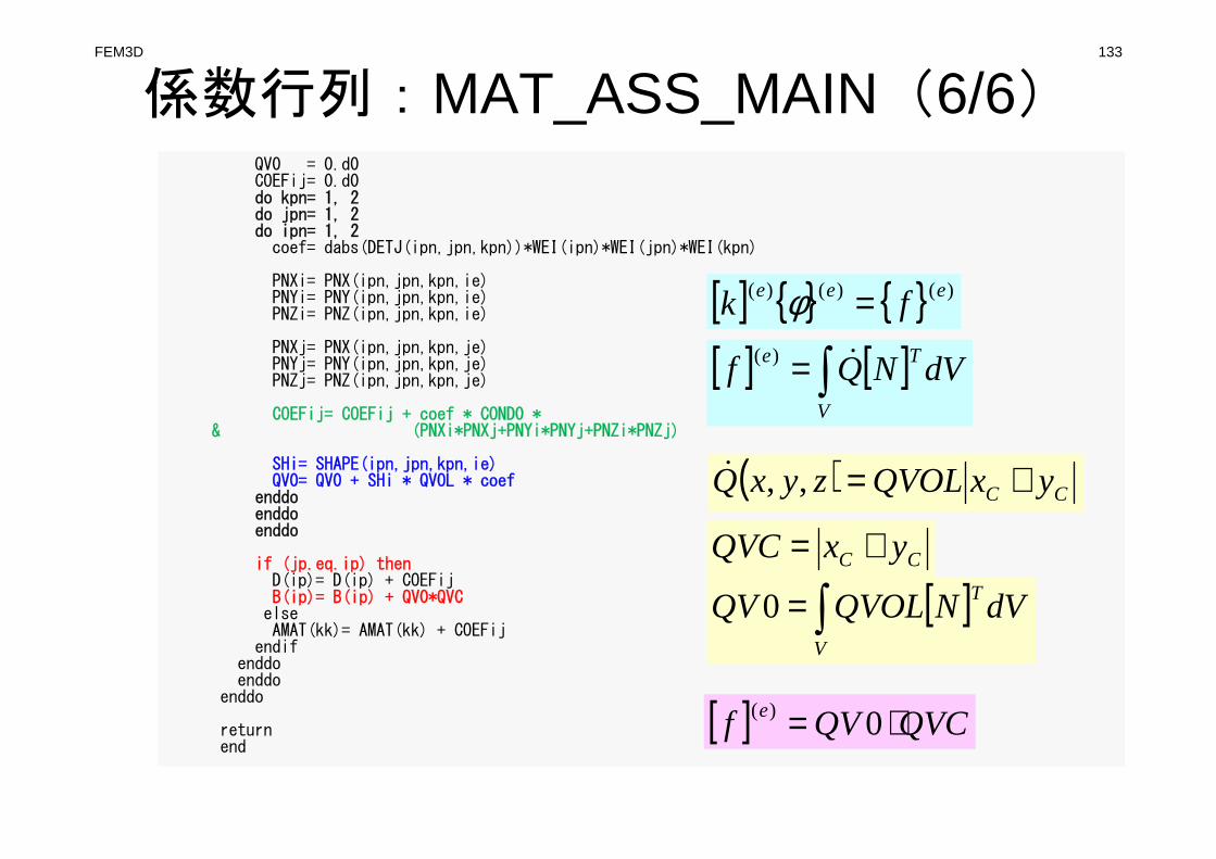
FEM3D 133
係数行列:MAT_ASS_MAIN(6/6)QV0 = 0.d0COEFij= 0.d0do kpn= 1, 2do jpn= 1, 2do ipn= 1, 2coef= dabs(DETJ(ipn,jpn,kpn))*WEI(ipn)*WEI(jpn)*WEI(kpn)
PNXi= PNX(ipn,jpn,kpn,ie)PNYi= PNY(ipn,jpn,kpn,ie)PNZi= PNZ(ipn,jpn,kpn,ie)
PNXj= PNX(ipn,jpn,kpn,je)PNYj= PNY(ipn,jpn,kpn,je)PNZj= PNZ(ipn,jpn,kpn,je)
COEFij= COEFij + coef * COND0 *& (PNXi*PNXj+PNYi*PNYj+PNZi*PNZj)
SHi= SHAPE(ipn,jpn,kpn,ie)QV0= QV0 + SHi * QVOL * coef
enddoenddoenddo
if (jp.eq.ip) thenD(ip)= D(ip) + COEFijB(ip)= B(ip) + QV0*QVC
elseAMAT(kk)= AMAT(kk) + COEFij
endifenddoenddo
enddo
returnend
[ ] { } { } )()()( eee fk =φ
[ ] [ ] dVNQfV
Te
∫= &
)(
( ) CC yxQVOLzyxQ +=,,&
CC yxQVC +=
[ ] dVNQVOLQVV
T
∫=0
[ ] QVCQVf e ⋅= 0)(

FEM3D 134
MAT_ASS_BC: Overview
do i= 1, N Loop for Nodes
“Mark” nodes where Dirichlet B.C. are applied (IWKX)
enddo
do i= 1, N Loop for Nodes
if (IWKX(i,1).eq.1) then if “marked” nodes
corresponding components of RHS (B), Diagonal (D) are correcteddo k= index(i-1)+1, index(i) Non-Zero Off-Diagonal Nodes
corresponding comp. of non-zero off-diagonal components (AMAT) are corrected
enddoendif
enddo
do i= 1, N Loop for Nodes
do k= index(i-1)+1, index(i) Non-Zero Off-Diagonal Nodes
if (IWKX(item(k),1).eq.1) then if corresponding non-zerooff-diagonal node is “marked”
corresponding components of RHS and AMAT are corrected (col.)
endifenddo
enddo
X
Y
Z
NYNX
NZ
T=0@Z=zmax
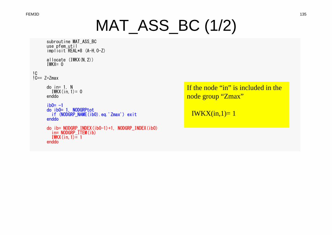
FEM3D 135
MAT_ASS_BC (1/2)subroutine MAT_ASS_BCuse pfem_utilimplicit REAL*8 (A-H,O-Z)
allocate (IWKX(N,2))IWKX= 0
!C!C== Z=Zmax
do in= 1, NIWKX(in,1)= 0
enddo
ib0= -1do ib0= 1, NODGRPtot
if (NODGRP_NAME(ib0).eq.'Zmax') exitenddo
do ib= NODGRP_INDEX(ib0-1)+1, NODGRP_INDEX(ib0)in= NODGRP_ITEM(ib)IWKX(in,1)= 1
enddo
If the node “in” is included in the node group “Zmax”
IWKX(in,1)= 1

FEM3D 136
MAT_ASS_BC (2/2)do in= 1, N
if (IWKX(in,1).eq.1) thenB(in)= 0.d0D(in)= 1.d0
iS= index(in-1) + 1iE= index(in )do k= iS, iEAMAT(k)= 0.d0
enddoendif
enddo
do in= 1, NiS= index(in-1) + 1iE= index(in )do k= iS, iE
if (IWKX(item(k),1).eq.1) thenAMAT(k)= 0.d0
endifenddo
enddo!C==
returnend

1D Steady State Heat Conduction
0=+
∂∂
∂∂
Qx
T
x&λ
• Uniform: Sectional Area: A, Thermal Conductivity: λ
• Heat Generation Rate/Volume/Time [QL-3T-1]
• Boundary Conditions– x=0 : T= 0 (Fixed Temperature)
– x=xmax: (Insulated)0=∂∂
x
T
Q&
x=0 (xmin) x= xmax
FEM3D 137
1D
heat generation/volume Q&

FEM1D 138
(Linear) Equation at x=0T1= 0 (or T0 = 0)
0=+
∂∂
∂∂
Qx
T
x&λ
x=0 (xmin) x= xmax
heat generation/volume Q&
• Uniform: Sectional Area: A, Thermal Conductivity: λ
• Heat Generation Rate/Volume/Time [QL-3T-1]
• Boundary Conditions– x=0 : T= 0 (Fixed Temperature)
– x=xmax: (Insulated)0=∂∂
x
T
Q&
1D

FEM1D 139
!C!C +---------------------+!C | BOUNDARY CONDITIONS |!C +---------------------+!C===
!C!C-- X=Xmin
i= 1jS= INDEX(i-1)
AMAT(jS+1)= 0.d0DIAG(i)= 1.d0RHS (i)= 0.d0
do k= 1, NPLUif (ITEM(k).eq.1) AMAT(k)= 0.d0
enddo!C===
Program: 1d.f (6/6) Dirichlet B.C. @ X=0
T1=0
Diagonal Component=1RHS=0Off-Diagonal Components= 0.
1D
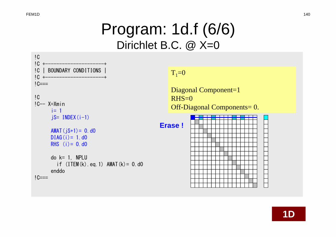
!C!C +---------------------+!C | BOUNDARY CONDITIONS |!C +---------------------+!C===
!C!C-- X=Xmin
i= 1jS= INDEX(i-1)
AMAT(jS+1)= 0.d0DIAG(i)= 1.d0RHS (i)= 0.d0
do k= 1, NPLUif (ITEM(k).eq.1) AMAT(k)= 0.d0
enddo!C===
FEM1D 140
Program: 1d.f (6/6) Dirichlet B.C. @ X=0
Erase !
T1=0
Diagonal Component=1RHS=0Off-Diagonal Components= 0.
1D

!C!C +---------------------+!C | BOUNDARY CONDITIONS |!C +---------------------+!C===
!C!C-- X=Xmin
i= 1jS= INDEX(i-1)
AMAT(jS+1)= 0.d0DIAG(i)= 1.d0RHS (i)= 0.d0
do k= 1, NPLUif (ITEM(k).eq.1) AMAT(k)= 0.d0
enddo!C===
FEM1D 141
Program: 1d.f (6/6) Dirichlet B.C. @ X=0
Elimination and Erase
Column components of boundary nodes (Dirichlet B.C.) are moved to RHS and eliminated for keeping symmetrical feature of the matrix (in this case just erase off-diagonal components)
T1=0
Diagonal Component=1RHS=0Off-Diagonal Components= 0.
1D
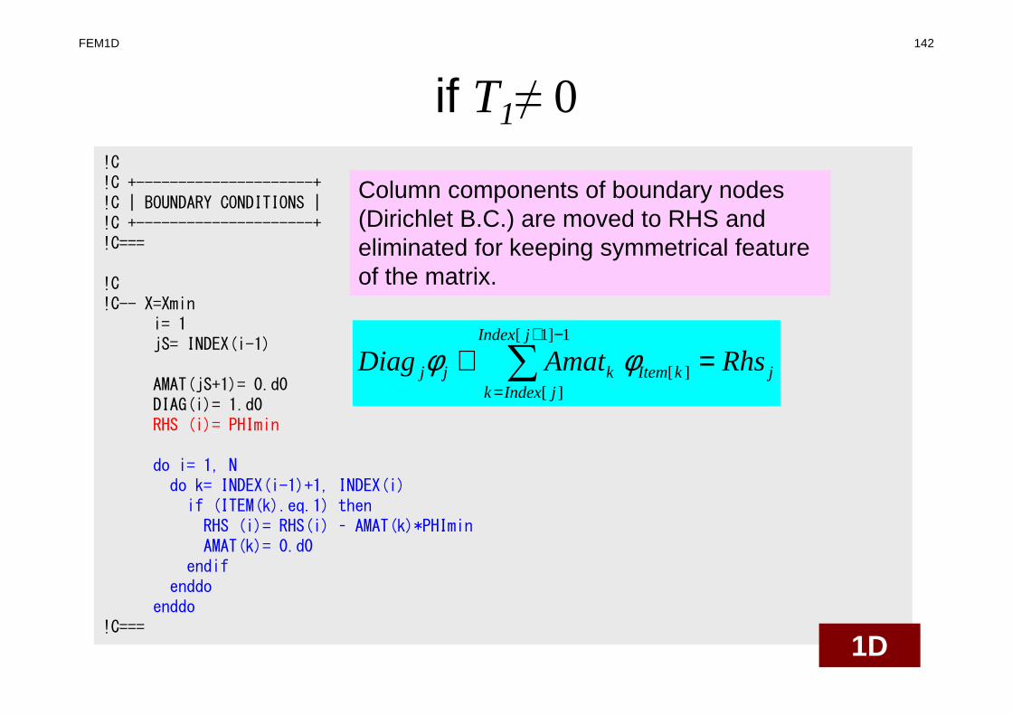
FEM1D 142
if T1≠ 0!C!C +---------------------+!C | BOUNDARY CONDITIONS |!C +---------------------+!C===
!C!C-- X=Xmin
i= 1jS= INDEX(i-1)
AMAT(jS+1)= 0.d0DIAG(i)= 1.d0RHS (i)= PHImin
do i= 1, Ndo k= INDEX(i-1)+1, INDEX(i)
if (ITEM(k).eq.1) thenRHS (i)= RHS(i) – AMAT(k)*PHIminAMAT(k)= 0.d0
endifenddo
enddo!C===
jkItem
jIndex
jIndexkkjj RhsAmatDiag =+ ∑
−+
=][
1]1[
][
φφ
Column components of boundary nodes (Dirichlet B.C.) are moved to RHS and eliminated for keeping symmetrical feature of the matrix.
1D

FEM1D 143
if T1≠ 0!C!C +---------------------+!C | BOUNDARY CONDITIONS |!C +---------------------+!C===
!C!C-- X=Xmin
i= 1jS= INDEX(i-1)
AMAT(jS+1)= 0.d0DIAG(i)= 1.d0RHS (i)= PHImin
do i= 1, Ndo k= INDEX(i-1)+1, INDEX(i)
if (ITEM(k).eq.1) thenRHS (i)= RHS(i) – AMAT(k)*PHIminAMAT(k)= 0.d0
endifenddo
enddo!C===
1][min
][
][
1]1[
],[
=−=
−=
+ ∑−+
≠=
skj
kItemkj
kItem
jIndex
kkjIndexkkjj
kItemwhereAmatRhs
AmatRhs
AmatDiag
s
ss
s
φφ
φφ
Column components of boundary nodes (Dirichlet B.C.) are moved to RHS and eliminated for keeping symmetrical feature of the matrix.
1D

FEM3D 144
MAT_ASS_BC (2/2)do in= 1, N
if (IWKX(in,1).eq.1) thenB(in)= 0.d0D(in)= 1.d0
iS= index(in-1) + 1iE= index(in )do k= iS, iEAMAT(k)= 0.d0
enddoendif
enddo
do in= 1, NiS= index(in-1) + 1iE= index(in )do k= iS, iE
if (IWKX(item(k),1).eq.1) thenAMAT(k)= 0.d0
endifenddo
enddo!C==
returnend
Same as 1D case
Erase !!
Boundary Nodes: IWKX(in,1)=1

FEM3D 145
MAT_ASS_BC (2/2)do in= 1, N
if (IWKX(in,1).eq.1) thenB(in)= 0.d0D(in)= 1.d0
iS= index(in-1) + 1iE= index(in )do k= iS, iEAMAT(k)= 0.d0
enddoendif
enddo
do in= 1, NiS= index(in-1) + 1iE= index(in )do k= iS, iE
if (IWKX(item(k),1).eq.1) thenAMAT(k)= 0.d0
endifenddo
enddo!C==
returnend
Elimination and Erase
Boundary Nodes: IWKX(in,1)=1
Same as 1D case

FEM3D 146
Structure of heat3D
test1main
input_cntlinput of control data
input_gridinput of mesh info
mat_con0connectivity of matrix
mat_con1connectivity of matrix
mat_ass_maincoefficient matrix
mat_ass_bcboundary conditions
solve11control of linear solver
output_ucdvisualization
mSORTsorting
jacobiJacobian
find_nodesearching nodes
cgCG solver

FEM3D 147
Main Partprogram heat3D
use solver11use pfem_util
implicit REAL*8(A-H,O-Z)
call INPUT_CNTLcall INPUT_GRID
call MAT_CON0call MAT_CON1
call MAT_ASS_MAINcall MAT_ASS_BC
call SOLVE11
call OUTPUT_UCD
end program heat3D

FEM3D 148
SOLVE11module SOLVER11
containssubroutine SOLVE11
use pfem_utiluse solver_CG
implicit REAL*8 (A-H,O-Z)
integer :: ERROR, ICFLAGcharacter(len=char_length) :: BUF
data ICFLAG/0/
!C!C +------------+!C | PARAMETERs |!C +------------+!C===
ITER = pfemIarray(1) Max. Iterations for CGRESID = pfemRarray(1) Convergence Criteria for CG
!C===!C!C +------------------+!C | ITERATIVE solver |!C +------------------+!C===
call CG && ( N, NPLU, D, AMAT, index, item, B, X, RESID, ITER, ERROR )
ITERactual= ITER!C===
end subroutine SOLVE11end module SOLVER11
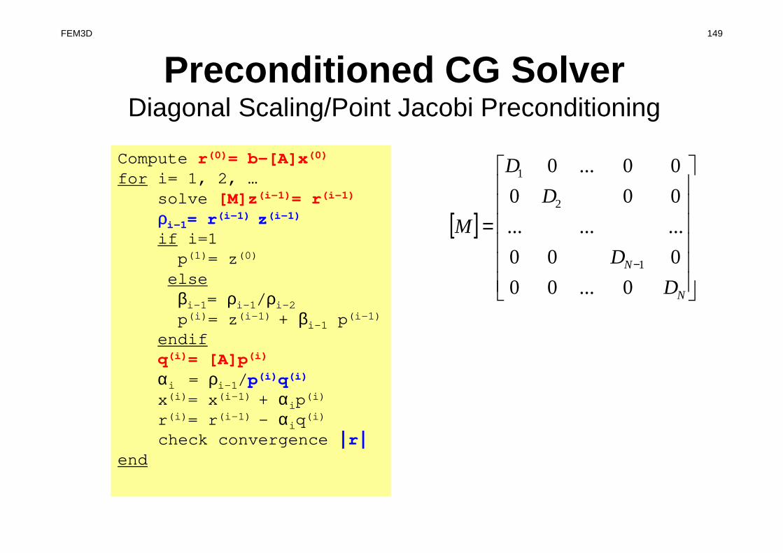
Preconditioned CG SolverDiagonal Scaling/Point Jacobi Preconditioning
FEM3D 149
Compute r(0)= b-[A]x(0)
for i= 1, 2, …solve [M]z(i-1)= r(i-1)
ρi-1= r(i-1) z(i-1)if i=1p(1)= z(0)
elseβi-1= ρi-1/ρi-2p(i)= z(i-1) + βi-1 p(i-1)
endifq(i)= [A]p(i)
αi = ρi-1/p(i)q(i)x(i)= x(i-1) + αip
(i)
r(i)= r(i-1) - αiq(i)
check convergence |r|end
[ ]
=
−
N
N
D
D
D
D
M
0...00
000
.........
000
00...0
1
2
1
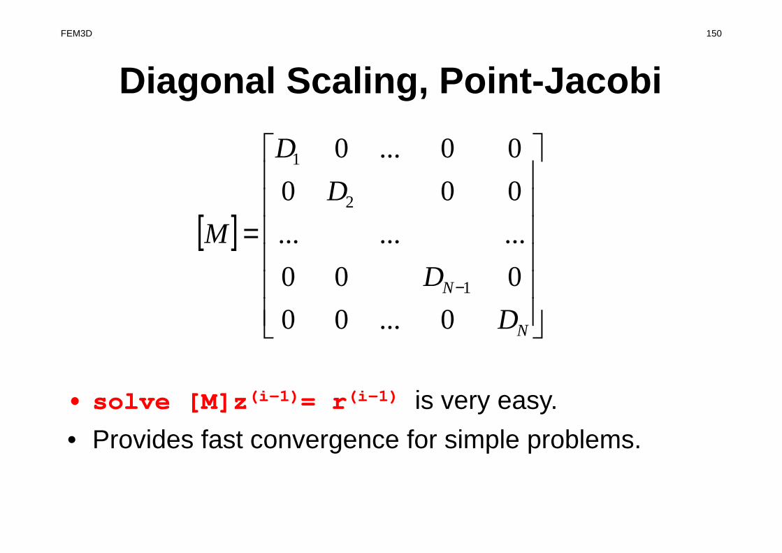
Diagonal Scaling, Point-Jacobi
FEM3D 150
• solve [M]z(i-1)= r(i-1) is very easy.
• Provides fast convergence for simple problems.
[ ]
=
−
N
N
D
D
D
D
M
0...00
000
.........
000
00...0
1
2
1
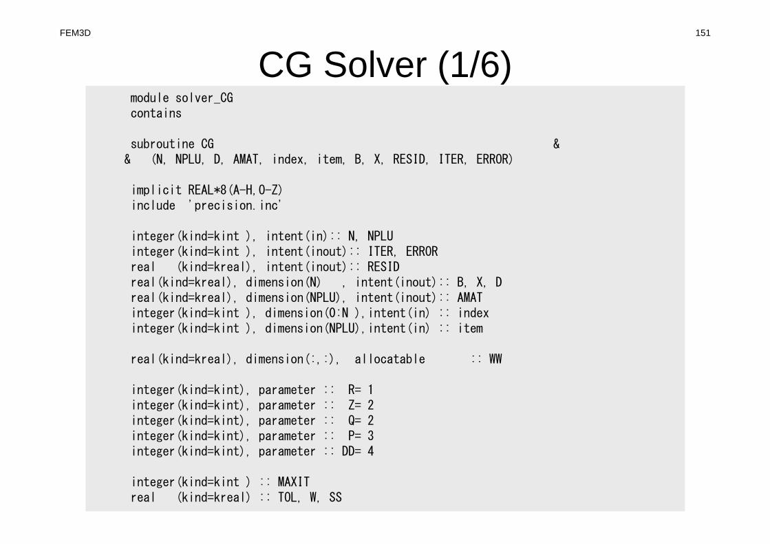
CG Solver (1/6)module solver_CGcontains
subroutine CG && (N, NPLU, D, AMAT, index, item, B, X, RESID, ITER, ERROR)
implicit REAL*8(A-H,O-Z)include 'precision.inc'
integer(kind=kint ), intent(in):: N, NPLUinteger(kind=kint ), intent(inout):: ITER, ERRORreal (kind=kreal), intent(inout):: RESIDreal(kind=kreal), dimension(N) , intent(inout):: B, X, Dreal(kind=kreal), dimension(NPLU), intent(inout):: AMATinteger(kind=kint ), dimension(0:N ),intent(in) :: indexinteger(kind=kint ), dimension(NPLU),intent(in) :: item
real(kind=kreal), dimension(:,:), allocatable :: WW
integer(kind=kint), parameter :: R= 1integer(kind=kint), parameter :: Z= 2integer(kind=kint), parameter :: Q= 2integer(kind=kint), parameter :: P= 3integer(kind=kint), parameter :: DD= 4
integer(kind=kint ) :: MAXITreal (kind=kreal) :: TOL, W, SS
FEM3D 151

CG Solver (1/6)module solver_CGcontains
subroutine CG && (N, NPLU, D, AMAT, index, item, B, X, RESID, ITER, ERROR)
implicit REAL*8(A-H,O-Z)include 'precision.inc'
integer(kind=kint ), intent(in):: N, NPLUinteger(kind=kint ), intent(inout):: ITER, ERRORreal (kind=kreal), intent(inout):: RESIDreal(kind=kreal), dimension(N) , intent(inout):: B, X, Dreal(kind=kreal), dimension(NPLU), intent(inout):: AMATinteger(kind=kint ), dimension(0:N ),intent(in) :: indexinteger(kind=kint ), dimension(NPLU),intent(in) :: item
real(kind=kreal), dimension(:,:), allocatable :: WW
integer(kind=kint), parameter :: R= 1integer(kind=kint), parameter :: Z= 2integer(kind=kint), parameter :: Q= 2integer(kind=kint), parameter :: P= 3integer(kind=kint), parameter :: DD= 4
integer(kind=kint ) :: MAXITreal (kind=kreal) :: TOL, W, SS
WW(i,1)= WW(i,R) ⇒ {r}WW(i,2)= WW(i,Z) ⇒ {z}WW(i,2)= WW(i,Q) ⇒ {q}WW(i,3)= WW(i,P) ⇒ {p}WW(i,4)= WW(i,DD) ⇒ 1/{D}
Compute r(0)= b-[A]x(0)
for i= 1, 2, …solve [M]z(i-1)= r(i-1)
ρi-1= r(i-1) z(i-1)if i=1p(1)= z(0)
elseβi-1= ρi-1/ρi-2p(i)= z(i-1) + βi-1 p(i-1)
endifq(i)= [A]p(i)
αi = ρi-1/p(i)q(i)x(i)= x(i-1) + αip
(i)
r(i)= r(i-1) - αiq(i)
check convergence |r|end
FEM3D 152

CG Solver (2/6)!C!C +-------+!C | INIT. |!C +-------+!C===
ERROR= 0allocate (WW(N,4))MAXIT = ITERTOL = RESIDX = 0.d0
!C===
!C +-----------------------+!C | {r0}= {b} - [A]{xini} |!C +-----------------------+!C===
do j= 1, NWW(j,DD)= 1.d0/D(j)WVAL= B(j) - D(j)*X(j)do k= index(j-1)+1, index(j)
i= item(k)WVAL= WVAL - AMAT(k)*X(i)
enddoWW(j,R)= WVAL
enddo
FEM3D 153
WW(i,1)= WW(i,R) ⇒ {r}WW(i,2)= WW(i,Z) ⇒ {z}WW(i,2)= WW(i,Q) ⇒ {q}WW(i,3)= WW(i,P) ⇒ {p}WW(i,4)= WW(i,DD) ⇒ 1/{D}
Reciprocal numbers (逆数)of diagonal components are stored in WW(i,DD).Computational cost for division is usually expensive.

CG Solver (2/6)!C!C +-------+!C | INIT. |!C +-------+!C===
ERROR= 0allocate (WW(N,4))MAXIT = ITERTOL = RESIDX = 0.d0
!C===
!C +-----------------------+!C | {r0}= {b} - [A]{xini} |!C +-----------------------+!C===
do j= 1, NWW(j,DD)= 1.d0/D(j)WVAL= B(j) - D(j)*X(j)do k= index(j-1)+1, index(j)
i= item(k)WVAL= WVAL - AMAT(k)*X(i)
enddoWW(j,R)= WVAL
enddo
Compute r(0)= b-[A]x(0)
for i= 1, 2, …solve [M]z(i-1)= r(i-1)
ρi-1= r(i-1) z(i-1)if i=1p(1)= z(0)
elseβi-1= ρi-1/ρi-2p(i)= z(i-1) + βi-1 p(i-1)
endifq(i)= [A]p(i)
αi = ρi-1/p(i)q(i)x(i)= x(i-1) + αip
(i)
r(i)= r(i-1) - αiq(i)
check convergence |r|end
FEM3D 154

CG Solver (3/6)BNRM20= 0.d0do i= 1, NBNRM20= BNRM20 + B(i)**2
enddo
BNRM2= BNRM20
if (BNRM2.eq.0.d0) BNRM2= 1.d0ITER = 0
!C===
do iter= 1, MAXIT!C!C************************************************* Conjugate Gradient Iteration
!C!C +----------------+!C | {z}= [Minv]{r} |!C +----------------+!C===
do i= 1, NWW(i,Z)= WW(i,R) * WW(i,DD)
enddo!C===
FEM3D 155
BNRM2=|b|2
for convergence criteria of CG solvers
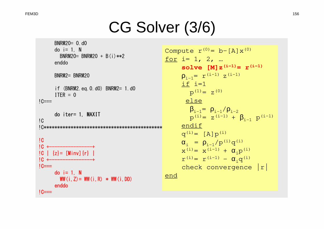
CG Solver (3/6)BNRM20= 0.d0do i= 1, NBNRM20= BNRM20 + B(i)**2
enddo
BNRM2= BNRM20
if (BNRM2.eq.0.d0) BNRM2= 1.d0ITER = 0
!C===
do iter= 1, MAXIT!C!C************************************************* Conjugate Gradient Iteration
!C!C +----------------+!C | {z}= [Minv]{r} |!C +----------------+!C===
do i= 1, NWW(i,Z)= WW(i,R) * WW(i,DD)
enddo!C===
Compute r(0)= b-[A]x(0)
for i= 1, 2, …solve [M]z(i-1)= r(i-1)
ρi-1= r(i-1) z(i-1)if i=1p(1)= z(0)
elseβi-1= ρi-1/ρi-2p(i)= z(i-1) + βi-1 p(i-1)
endifq(i)= [A]p(i)
αi = ρi-1/p(i)q(i)x(i)= x(i-1) + αip
(i)
r(i)= r(i-1) - αiq(i)
check convergence |r|end
FEM3D 156

CG Solver (4/6)!C!C +---------------+!C | {RHO}= {r}{z} |!C +---------------+!C===
RHO0= 0.d0do i= 1, NRHO0= RHO0 + WW(i,R)*WW(i,Z)
enddoRHO= RHO0
!C===!C +-----------------------------+!C | {p} = {z} if ITER=1 |!C | BETA= RHO / RHO1 otherwise |!C +-----------------------------+!C===
if ( ITER.eq.1 ) thendo i= 1, N
WW(i,P)= WW(i,Z)enddoelse
BETA= RHO / RHO1do i= 1, N
WW(i,P)= WW(i,Z) + BETA*WW(i,P)enddo
endif!C===
Compute r(0)= b-[A]x(0)
for i= 1, 2, …solve [M]z(i-1)= r(i-1)
ρi-1= r(i-1) z(i-1)if i=1p(1)= z(0)
elseβi-1= ρi-1/ρi-2p(i)= z(i-1) + βi-1 p(i-1)
endifq(i)= [A]p(i)
αi = ρi-1/p(i)q(i)x(i)= x(i-1) + αip
(i)
r(i)= r(i-1) - αiq(i)
check convergence |r|end
FEM3D 157

CG Solver (5/6)!C +-------------+!C | {q}= [A]{p} |!C +-------------+!C===
do j= 1, NWVAL= D(j)*WW(j,P)do k= index(j-1)+1, index(j)
i= item(k)WVAL= WVAL + AMAT(k)*WW(i,P)
enddoWW(j,Q)= WVAL
enddo!C===!C +---------------------+!C | ALPHA= RHO / {p}{q} |!C +---------------------+!C===
C10= 0.d0do i= 1, NC10= C10 + WW(i,P)*WW(i,Q)
enddoC1= C10ALPHA= RHO / C1
!C===
Compute r(0)= b-[A]x(0)
for i= 1, 2, …solve [M]z(i-1)= r(i-1)
ρi-1= r(i-1) z(i-1)if i=1p(1)= z(0)
elseβi-1= ρi-1/ρi-2p(i)= z(i-1) + βi-1 p(i-1)
endifq(i)= [A]p(i)
αi = ρi-1/p(i)q(i)x(i)= x(i-1) + αip
(i)
r(i)= r(i-1) - αiq(i)
check convergence |r|end
FEM3D 158

CG Solver (6/6)!C!C +----------------------+!C | {x}= {x} + ALPHA*{p} |!C | {r}= {r} - ALPHA*{q} |!C +----------------------+!C===
do i= 1, NX(i) = X (i) + ALPHA * WW(i,P)
WW(i,R)= WW(i,R) - ALPHA * WW(i,Q)enddo
!C===DNRM20= 0.d0do i= 1, N
DNRM20= DNRM20 + WW(i,R)**2enddoDNRM2= DNRM20RESID= dsqrt(DNRM2/BNRM2)
if ( RESID.le.TOL ) exitif ( ITER .eq.MAXIT ) ERROR= -300
RHO1 = RHOenddo
!C===
Compute r(0)= b-[A]x(0)
for i= 1, 2, …solve [M]z(i-1)= r(i-1)
ρi-1= r(i-1) z(i-1)if i=1p(1)= z(0)
elseβi-1= ρi-1/ρi-2p(i)= z(i-1) + βi-1 p(i-1)
endifq(i)= [A]p(i)
αi = ρi-1/p(i)q(i)x(i)= x(i-1) + αip
(i)
r(i)= r(i-1) - αiq(i)
check convergence |r|end
FEM3D 159

CG Solver (6/6)!C!C +----------------------+!C | {x}= {x} + ALPHA*{p} |!C | {r}= {r} - ALPHA*{q} |!C +----------------------+!C===
do i= 1, NX(i) = X (i) + ALPHA * WW(i,P)
WW(i,R)= WW(i,R) - ALPHA * WW(i,Q)enddo
!C===DNRM20= 0.d0do i= 1, N
DNRM20= DNRM20 + WW(i,R)**2enddoDNRM2= DNRM20RESID= dsqrt(DNRM2/BNRM2)
if ( RESID.le.TOL ) exitif ( ITER .eq.MAXIT ) ERROR= -300
RHO1 = RHOenddo
!C===
Compute r(0)= b-[A]x(0)
for i= 1, 2, …solve [M]z(i-1)= r(i-1)
ρi-1= r(i-1) z(i-1)if i=1p(1)= z(0)
elseβi-1= ρi-1/ρi-2p(i)= z(i-1) + βi-1 p(i-1)
endifq(i)= [A]p(i)
αi = ρi-1/p(i)q(i)x(i)= x(i-1) + αip
(i)
r(i)= r(i-1) - αiq(i)
check convergence |r|end
TolBNorm2
DNorm2Resid ≤
−===
b
bAx
b
r
FEM3D 160