3.11 - Method of Images - MIT OpenCourseWare · PDF fileB Gauss outward υB Archimedes...
10
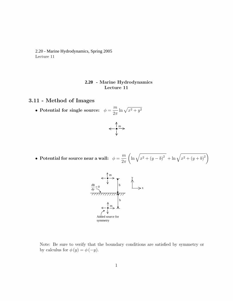
Lecture 11 - Marine Hydrodynamics Lecture 11 3.11 - Method of Images m • Potential for single source: φ = ln x 2 + y 2 2π m • Potential for source near a wall: φ = m ln x 2 +(y − b) 2 + ln x 2 +(y + b) 2 2π b b Added source for 0 = φ dy d x y m m symmetry Note: Be sure to verify that the boundary conditions are satisfied by symmetry or by calculus for φ (y)= φ (−y). 1 2.20 - Marine Hydrodynamics, Spring 2005 2.20
Transcript of 3.11 - Method of Images - MIT OpenCourseWare · PDF fileB Gauss outward υB Archimedes...
m
m
( √ √ )
Lecture 11
- Marine Hydrodynamics Lecture 11
3.11 - Method of Images m √
• Potential for single source: φ = ln x2 + y2
2π
m
• Potential for source near a wall: φ = m
ln x2 + (y − b)2 + ln x2 + (y + b)2
2π
b
b
Added source for
0= φ dy
d x
y
m
m
symmetry
Note: Be sure to verify that the boundary conditions are satisfied by symmetry or by calculus for φ (y) = φ (−y).
1
2.20 - Marine Hydrodynamics, Spring 2005
2.20
( )
( )
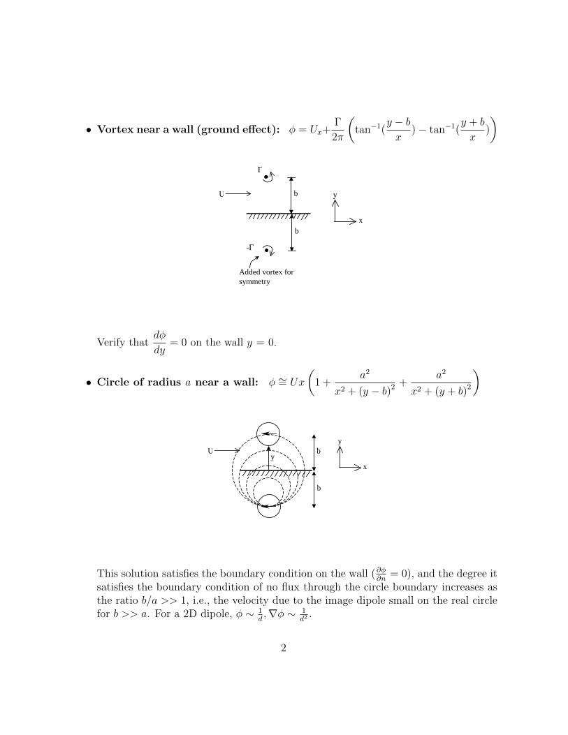
• Vortex near a wall (ground effect): φ = Ux+ Γ
tan−1(y − b
) − tan−1(y + b
)2π x x
b
b
Γ
U
x
y
-Γ
Added vortex for symmetry
dφ Verify that = 0 on the wall y = 0.
dy
2 2
φ ∼ a a • Circle of radius a near a wall: = Ux 1 + + x2 + (y − b)2 x2 + (y + b)2
b
bU y
x
y
This solution satisfies the boundary condition on the wall (∂φ = 0), and the degree it ∂n
satisfies the boundary condition of no flux through the circle boundary increases as the ratio b/a >> 1, i.e., the velocity due to the image dipole small on the real circle for b >> a. For a 2D dipole, φ ∼
d1 , ∇φ ∼
d1 2 .
2
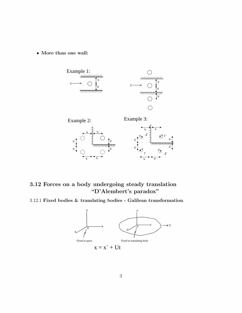
• More than one wall:
b'
b U
b'
b U
b'
Example 1:
Example 2: Example 3:
bb bb
-Γ Γ b'
b' b'b'
b'b'b'b'
Γ -Γ b b b b
3.12 Forces on a body undergoing steady translation “D’Alembert’s paradox”
3.12.1 Fixed bodies & translating bodies - Galilean transformation.
y y’
x’ Uo’x o z’ z
Fixed in space Fixed in translating body
x = x` + Ut
3
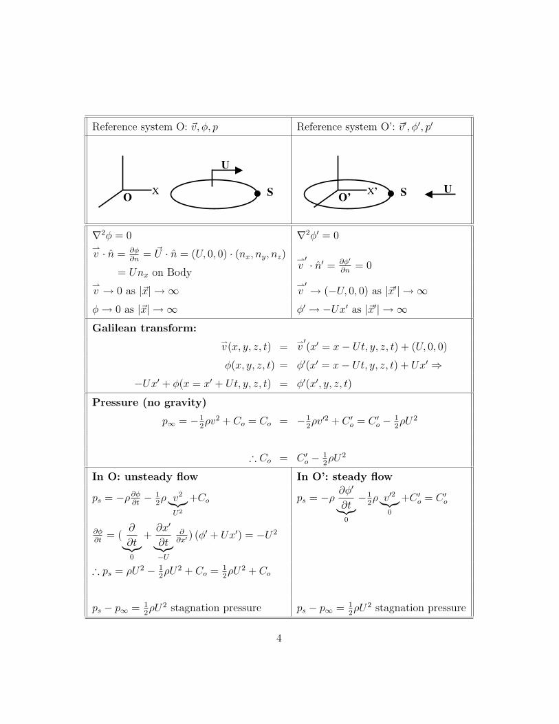
Reference system O: �v, φ, p Reference system O’: �v′, φ′, p′
U
SO
X USO’
X’
∇2φ = 0 ⇀ v · n = ∂φ
∂n = �U · n = (U, 0, 0) · (nx, ny, nz
= Unx on Body ⇀ v → 0 as |�x| → ∞
φ → 0 as |�x| → ∞
)
∇2φ′ = 0
⇀ v ′ · n′ = ∂φ′
∂n = 0
⇀ v ′ → (−U, 0, 0) as |�x′| → ∞
φ′ → −Ux′ as |�x′| → ∞
Galilean transform: ⇀ v(x, y, z, t)
φ(x, y, z, t)
−Ux′ + φ(x = x′ + Ut, y, z, t)
= ⇀ v ′ (x′ = x − Ut, y, z, t) + (U, 0, 0)
= φ′(x′ = x − Ut, y, z, t) + Ux′ ⇒
= φ′(x′, y, z, t)
Pressure (no gravity)
p∞ = −1 2 ρv2 + Co = Co
∴ Co
= −1 2 ρv′2 + C ′
o = C ′ o − 1
2 ρU2
= C ′ o − 1
2 ρU2
In O: unsteady flow
ps = −ρ∂φ ∂t − 1
2 ρ v2 ︸︷︷︸ U2
+Co
∂φ ∂t = (
∂ ∂t ︸︷︷︸ 0
+ ∂x′
∂t ︸︷︷︸ −U
∂ ∂x′ ) (φ′ + Ux′) = −U2
∴ ps = ρU2 − 1 2 ρU2 + Co = 1
2 ρU2 + Co
ps − p∞ = 1 2 ρU2 stagnation pressure
In O’: steady flow
ps = −ρ ∂φ′
∂t ︸︷︷︸ 0
−1 2 ρ v′2 ︸︷︷︸
0
+C ′ o = C ′
o
ps − p∞ = 1 2 ρU2 stagnation pressure
4
∫∫
⇀
⇀
⇀
⇀
∫∫
( )
∫∫ ∫∫∫ ∫∫∫
∫∫ ( )
( )
∫∫
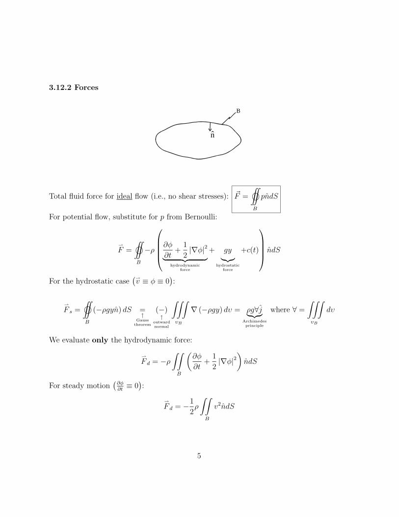
3.12.2 Forces
B
n
Total fluid force for ideal flow (i.e., no shear stresses): F� ndS= © pˆ
B
For potential flow, substitute for p from Bernoulli: ⎛ ⎞
⎜ ⎟ ⇀ ⎜∂φ 1 2 ⎟F = ©−ρ ⎜ + |∇φ| + gy +c(t)⎟ ndSˆ ⎝ ∂t 2 ⎠ ︸ ︷︷ ︸ ︸︷︷︸
B hydrodynamic hydrostatic
force force
For the hydrostatic case v ≡ φ ≡ 0 :
F s = © (−ρgyn) dS = (−) ∇ (−ρgy) dυ = ρg∀j where ∀ = dυ ↑ ︸︷︷︸ ↑
B Gauss outward υB Archimedes υBtheorem normal principle
We evaluate only the hydrodynamic force:
∂φ 1 2F d = −ρ + |∇φ| ndS ∂t 2
B
For steady motion ∂φ ≡ 0 :∂t
1 F d = − ρ 2 ˆv ndS
2 B
5
⇀ ∫ (
∣ ∣ ∣ ∣ ∣ ∣ ∣
∫ ( )
⇀
∫
( )
( ∣ ∣ ∣ ∣)
︸︷︷︸ ︸ ︷︷ ︸
∣ ∣
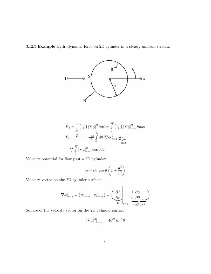
3.12.3 Example Hydrodynamic force on 2D cylinder in a steady uniform stream.
n
B
SU
a
x
2π
0 F d =
B
)ρ |∇ |φ
∫2π
i = −ρa
2 2− 2
−ρ2 |∇φ|nd� =ˆ nadθ r=a
2 idθ |∇φ|Fx F n· ·=2 r=a ︸︷︷︸
0 − cos θ
= ρa 2
2π
0
2|∇φ| cos θdθr=a
Velocity potential for flow past a 2D cylinder:
2a φ = Ur cos θ 1 +
2r
Velocity vector on the 2D cylinder surface:
∂φ 1 ∂φr ∂θ
∇φ| = (vr| , vθ| ) =r=a r=a r=a ,∂r r=a 0 r=a −2U sin θ
Square of the velocity vector on the 2D cylinder surface:
|∇φ|2 = 4U2 sin2 θ r=a
6
∫ ∫
∫
Finally, the hydrodynamic force on the 2D cylinder is given by
2π 2π ρa ( ) (1 )
Fx = dθ 4U2 sin2 θ cos θ = ρU2 (2a) 2 dθ sin2 θ cos θ = 0 2 2 ︸︷︷︸ ︸ ︷︷ ︸ ︸︷︷︸ ︸ ︷︷ ︸ odd 0 diameter 0 even
π 3π ps−p∞ or
w.r.t 2 , 2
projection ︸ ︷︷ ︸ ≡0
Therefore, Fx = 0 ⇒ no horizontal force ( symmetry fore-aft of the streamlines). Similarly,
2π (1 ) Fy = ρU2 (2a)2 dθ sin2 θ sin θ = 0
2 0
In fact, in general we find that F� ≡ 0, on any 2D or 3D body.
D’Alembert’s “paradox”:
No hydrodynamic force∗ acts on a body moving with steady translational (no circulation) velocity in an infinite, inviscid, irrotational fluid.
∗ The moment as measured in a local frame is not necessarily zero.
7
3.13 Lift due to Circulation
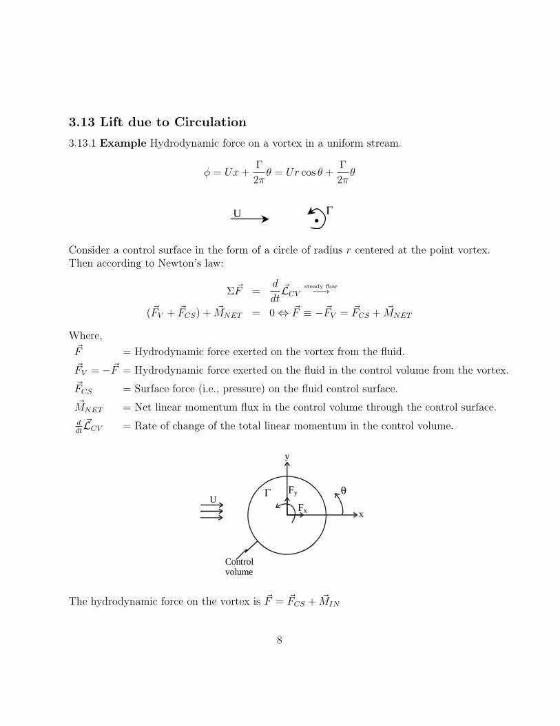
3.13.1 Example Hydrodynamic force on a vortex in a uniform stream.
Γ Γ φ = Ux + θ = Ur cos θ + θ
2π 2π
U Γ
Consider a control surface in the form of a circle of radius r centered at the point vortex. Then according to Newton’s law:
� d � steady flow ΣF = LCV −→
dt (F�
V + F� CS) + M�
NET = 0 ⇔ F� ≡ − F� V = F�
CS + M� NET
Where,
F� = Hydrodynamic force exerted on the vortex from the fluid.
F� V = − F� = Hydrodynamic force exerted on the fluid in the control volume from the vortex.
F� CS = Surface force (i.e., pressure) on the fluid control surface.
M� NET = Net linear momentum flux in the control volume through the control surface.
d L� CV = Rate of change of the total linear momentum in the control volume.
dt
Control volume
x
U
y
θFy
Fx
Γ
The hydrodynamic force on the vortex is F� = F� CS + M�
IN
8
∫ ∫ ( )
∫ ∫ ( )
∫
a. Net linear momentum flux in the control volume through the control surfaces, M� NET .
Recall that the control surface has the form of a circle of radius r centered at the point vortex.
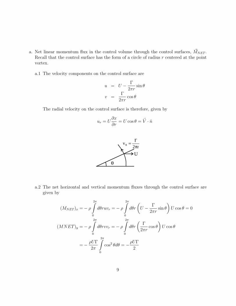
a.1 The velocity components on the control surface are
Γu = U − sin θ
2πr Γ
v = cos θ 2πr
The radial velocity on the control surface is therefore, given by
∂x ⇀
ur = U = U cos θ = V · n∂r
Γ vθ =
2πr
U
θ
a.2 The net horizontal and vertical momentum fluxes through the control surface are given by
2π 2π
Γ (MNET )x = − ρ dθruvr = − ρ dθr U − sin θ U cos θ = 0
2πr 0 0
2π 2π
Γ (MNET )y = − ρ dθrvvr = − ρ dθr cos θ U cos θ
2πr 0 0
2π ρUΓ ρUΓ
= − cos 2 θdθ = − 2π 2
0
9
( ) ( )( )
∫∫︸ ︷︷ ︸
( ) ∑
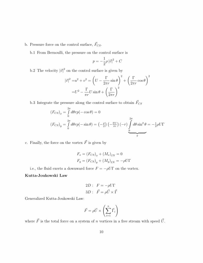
b. Pressure force on the control surface, F� CS.
b.1 From Bernoulli, the pressure on the control surface is
p = − 1 ρ |�v|2 + C
2
b.2 The velocity | |�v 2 on the control surface is given by 2 2
Γ Γ |�v|2 =u 2 + v 2 = U − sin θ + cos θ 2πr 2πr
2Γ Γ
=U2 − U sin θ + πr 2πr
b.3 Integrate the pressure along the control surface to obtain F� CS
2π
(FCS) = dθrp(− cos θ) = 0x 0
2π 2π∫ ( ) ( )
(FCS)y = dθrp(− sin θ) = −2 ρ −Γ
πrU (−r) dθ sin2 θ = −
21 ρUΓ
0 0
π
c. Finally, the force on the vortex F� is given by
Fx = (FCS)x + (Mx)IN = 0
Fy = (FCS) + (My)IN = −ρUΓ y
i.e., the fluid exerts a downward force F = −ρUΓ on the vortex.
Kutta-Joukowski Law
2D : F = −ρUΓ
3D : F� = ρU� × �Γ
Generalized Kutta-Joukowski Law:
n
F� = ρU� × �Γi
i=1
where F� is the total force on a system of n vortices in a free stream with speed U� .
10


![Introduction - University of California, Riversidemath.ucr.edu/~kelliher/papers/StokesEigenvalues.pdf · To prove Theorem 1.1 we adapt Filonov’s proof in [6] ... Let n be the outward-directed](https://static.fdocument.org/doc/165x107/5a8886f87f8b9a882e8e4456/introduction-university-of-california-kelliherpapersstokeseigenvaluespdfto.jpg)