
3. SEEMINGLY UNRELATED REGRESSIONS (SUR)
35
SUR-1 3. SEEMINGLY UNRELATED REGRESSIONS (SUR) [1] Examples • Demand for some commodities: y Nike,t = x Nike,t ′β Nike + ε Nike,t y Reebok,t = x Reebok,t ′β Reebok + ε Reebok,t ; where y Nike,t is the quantity demanded for Nike sneakers, x Nike,t is an 1×k Nike vector of regressors such as the unit price of Nike sneakers, prices of other sneakers, income ... , and t indexes time. • Household consumption expenditures on housing, clothing, and food. • Grunfeld’s investment data: • I: gross investment ($million) • F: market value of firm at the end of previous year. • C: value of firm’s capital at the end of previous year. • I it = β 1i + β 2i F it + β 3i C it + ε it , where i = GM, CH (Chrysler), GE, etc. • Notice that although the same regressors are used for each i, the values of the regressors are different across different i.
Transcript of 3. SEEMINGLY UNRELATED REGRESSIONS (SUR)
SUR-1
3. SEEMINGLY UNRELATED REGRESSIONS (SUR)
[1] Examples
• Demand for some commodities:
yNike,t = xNike,t′βNike + εNike,t
yReebok,t = xReebok,t′βReebok + εReebok,t;
where yNike,t is the quantity demanded for Nike sneakers, xNike,t is an 1×kNike
vector of regressors such as the unit price of Nike sneakers, prices of other
sneakers, income ... , and t indexes time.
• Household consumption expenditures
on housing, clothing, and food.
• Grunfeld’s investment data:
• I: gross investment ($million)
• F: market value of firm at the end of previous year.
• C: value of firm’s capital at the end of previous year.
• Iit = β1i + β2iFit + β3iCit + εit, where i = GM, CH (Chrysler), GE, etc.
• Notice that although the same regressors are used for each i, the values of
the regressors are different across different i.
• CAPM (Capital Asset Pricing Model)
• rit - rft: excess return on security i over a risk-free security.
• rmt-rft: excess market return.
• rit-rft = αi + βi(rmt-rft) + εit.
• Notice that the values of regressors are the same for every security.
• VAR (Vector Autoregressions)
• gCPI,t = growth rate of CPI (inflation rate)
• gGDP,t = growth rate of norminal GDP
• gCPI,t = αCPI + βCPIgCPI,t-1 + γCPIgGDP,t-1 + εCPI,t
gGDP,t = αGDP + βGDPgCPI,t-1 + γGDPgGDP,t-1 + εGDP,t
• Notice that the values of regressors are the same.
• Cobb-Douglas Cost function system
• Cost function is a function of output and input prices.
• Assume M inputs (labor, capital, land, material, energy, etc).
• Cobb-Douglas Cost function:
1ln ln ln( )My j j jC Y P cα β β== + + Σ + ε . (CD.1)
• Share functions (sj = pjxj/C, where xj = quantity of input j used)
lnlnj j
j
CsP jβ ε∂
= = +∂
, j = 1, ..., M. (CD.2)
• Observe that . This implies that 1 1Mj js=Σ = 1 1M
j jβ=Σ = and . 1 0Mj jε=Σ =
SUR-2
• Translog Cost function System
• Assume three inputs (j = 1, 2, and 3 index inputs, capital (k), labor (l), and
fuel (f), respectively.
• Translog cost function:
3 3 31 1 1
3 21 ,
ln ln .5 ln ln
ln ln ln .5 (ln )j j j j i ji j i
j y j j y yy c
C P P P
P Y Y Y
α β δ
γ θ θ= = =
=
= + Σ + Σ Σ
+Σ + + + ε, (T.1)
where δji = δij. (See Greene Ch. 14.)
• This is a generalization of Cobb-Douglas cost function.
• If the production function is homothetic, γy,1 = γy,2 = γy,3 = 0.
• If the production function is Cobb-Douglas,
δji = 0, γy,j = 0, θyy = 0, for all j and i.
• If the production function is Cobb-Douglas and constant returns to
scale,
δji = 0, γy,j = 0, θyy = 0, for all j and i; and θy = 1.
• Share functions:
31 1 1 1 ,1
1
32 2 1 2 ,2
2
33 3 1 3 ,3
3
ln ln ln ;lnln ln ln ;lnln ln ln .ln
i i i y
i i i y
i i i y
Cs PPCs PPCs PP
1
2
3
Y
Y
Y
β δ γ ε
β δ γ ε
β δ γ
=
=
=
∂= = + Σ + +∂∂
= = + Σ + +∂∂
= = + Σ + +∂
ε
(T.2)
• Note that . Thus, 1 2 3 1s s s+ + =
. 3 3 3 31 1 1 , 11; 0; 0; 0j j j ji j y j j jβ δ γ ε= = = =Σ = Σ = Σ = Σ =
SUR-3
SUR-4
[2] Basic Model
• Model: y1 = X1β1 + ε1;
y2 = X2β2 + ε2;
:
yn = Xnβn + εn,
where yi = T×1, Xi = T×ki, βi = ki×1, εi = (εi1 , ... , εiT)′ = T×1, and i = 1, ... , n.
• For a while, assume that there is no restrictions on β1, … , βn.
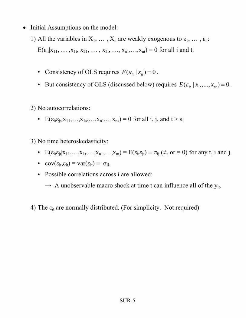
• Initial Assumptions on the model:
1) All the variables in X1, … , Xn are weakly exogenous to ε1, … , εn:
E(εit|x11, … ,x1t, x21, … , x2t, …, xn1,…,xnt) = 0 for all i and t.
• Consistency of OLS requires ( | ) 0it itE xε = .
• But consistency of GLS (discussed below) requires 1( | ,..., ) 0it t ntE x xε = .
2) No autocorrelations:
• E(εitεjs|x11,…,x1s,…,xn1,…xns) = 0 for all i, j, and t > s.
3) No time heteroskedasticity:
• E(εitεjt|x11,…,x1t,…,xn1,…,xnt) = E(εitεjt) ≡ σij (≠, or = 0) for any t, i and j.
• cov(εit,εit) = var(εit) ≡ σii.
• Possible correlations across i are allowed:
→ A unobservable macro shock at time t can influence all of the yit.
4) The εit are normally distributed. (For simplicity. Not required)
SUR-5
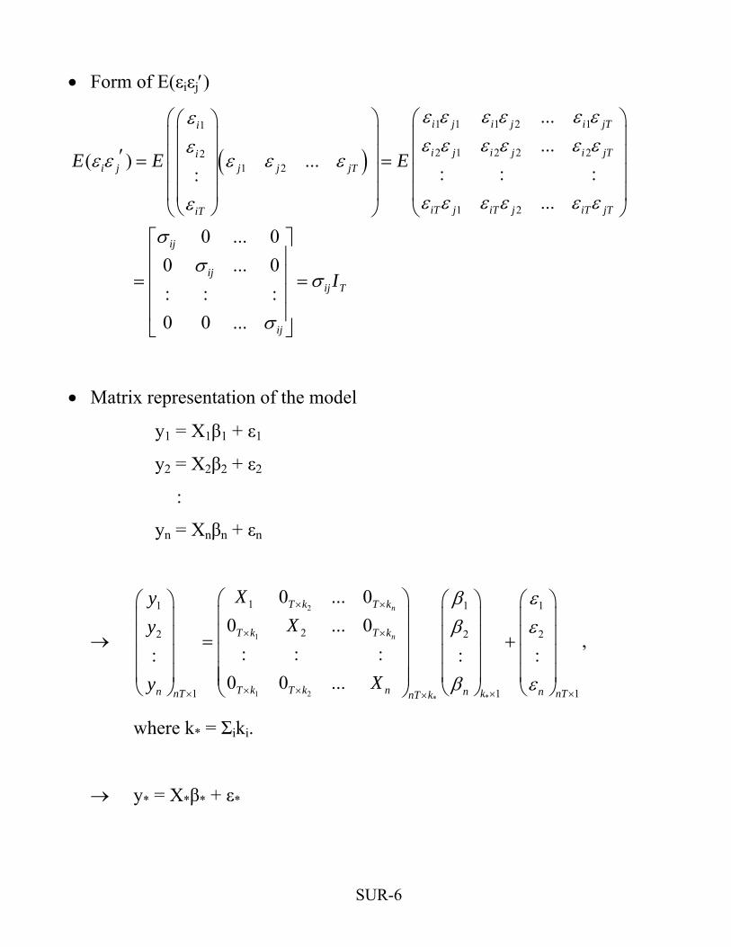
• Form of E(εiεj′)
( )1 1 1 2 11
2 1 2 2 221 2
1 2
...
...( ) ...
: : ::...
0 ... 00 ... 0: : :0 0 ...
i j i j i jTi
i j i j i jTii j j j jT
iT j iT j iT jTiT
ij
ijij T
ij
E E E
I
ε ε ε ε ε εεε ε ε ε ε εε
ε ε ε ε ε
ε ε ε ε ε εε
σσ
σ
σ
⎛ ⎞ ⎛ ⎞⎛ ⎞⎜ ⎟ ⎜ ⎟⎜ ⎟⎜ ⎟ ⎜ ⎟′ ⎜ ⎟= =⎜ ⎟ ⎜ ⎟⎜ ⎟⎜ ⎟ ⎜ ⎟⎜ ⎟⎝ ⎠ ⎝ ⎠⎝ ⎠
⎡ ⎤⎢ ⎥⎢ ⎥= =⎢ ⎥⎢ ⎥⎣ ⎦
• Matrix representation of the model
y1 = X1β1 + ε1
y2 = X2β2 + ε2
:
yn = Xnβn + εn
→ ,
2
1
1 2 **
11 1
22 2
1 1
0 ... 00 ... 0
: : :: :0 0 ...
n
n
T k T k
T k T k
T k T k nn nnT k nTnT k
XyXy
Xy
β εβ ε
β ε
× ×
× ×
× ×× ××
⎛ ⎞⎛ ⎞ ⎛ ⎞ ⎛ ⎞⎜ ⎟⎜ ⎟ ⎜ ⎟ ⎜ ⎟⎜ ⎟⎜ ⎟ ⎜ ⎟ ⎜ ⎟= +⎜ ⎟⎜ ⎟ ⎜ ⎟ ⎜ ⎟⎜ ⎟⎜ ⎟ ⎜ ⎟ ⎜ ⎟⎜ ⎟⎝ ⎠ ⎝ ⎠ ⎝ ⎠⎝ ⎠
1
2
1
:
n ×
where k* = Σiki.
→ y* = X*β* + ε*
SUR-6
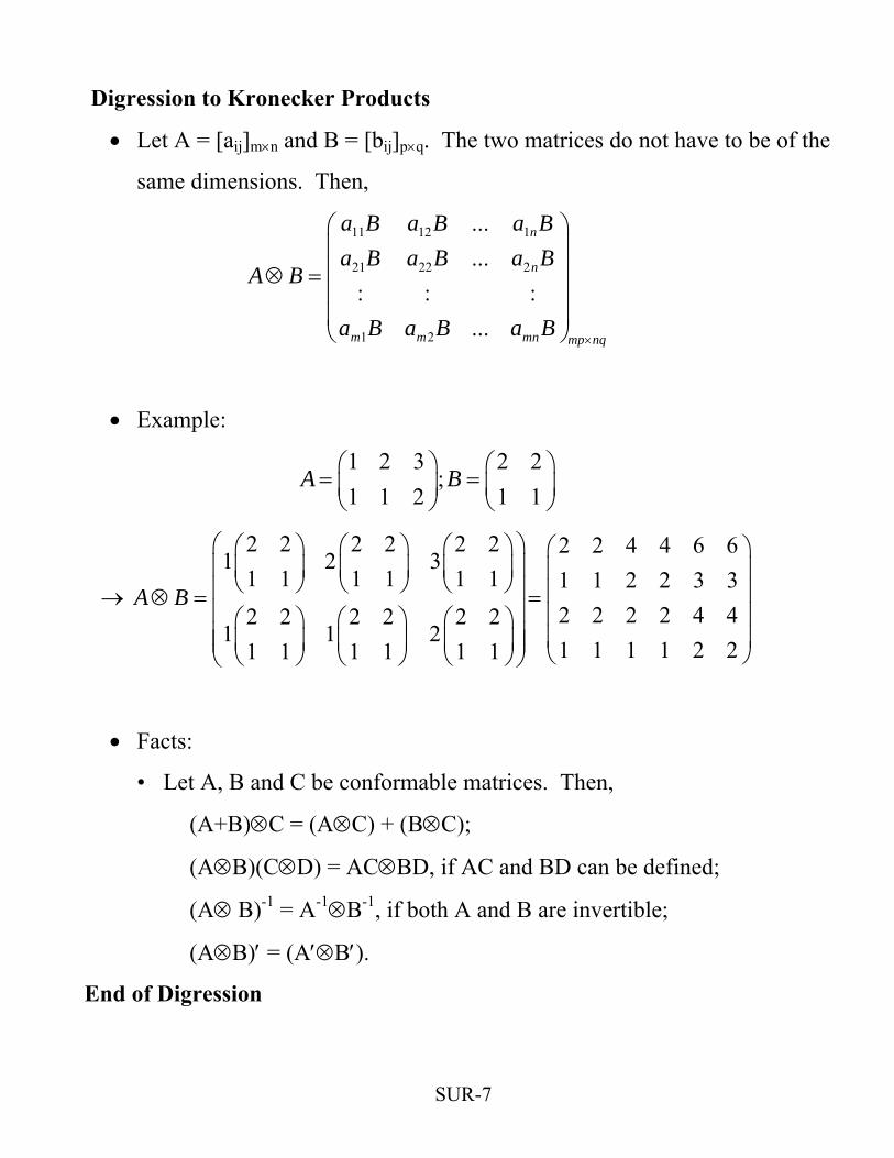
Digression to Kronecker Products
• Let A = [aij]m×n and B = [bij]p×q. The two matrices do not have to be of the
same dimensions. Then,
11 12 1
21 22 2
1 2
...
...: : :
...
n
n
m m mn mp nq
a B a B a Ba B a B a B
A B
a B a B a B×
⎛ ⎞⎜ ⎟⎜ ⎟⊗ =⎜ ⎟⎜ ⎟⎝ ⎠
• Example:
1 2 3 2 2
;1 1 2 1 1
A B⎛ ⎞ ⎛= =⎜ ⎟ ⎜⎝ ⎠ ⎝
⎞⎟⎠
→
2 2 2 2 2 2 2 2 4 4 6 61 2 3
1 1 1 1 1 1 1 1 2 2 3 32 2 2 2 4 42 2 2 2 2 2
1 1 21 1 1 1 2 21 1 1 1 1 1
A B
⎛ ⎞⎛ ⎞ ⎛ ⎞ ⎛ ⎞ ⎛ ⎞⎜ ⎟⎜ ⎟ ⎜ ⎟ ⎜ ⎟ ⎜ ⎟⎝ ⎠ ⎝ ⎠ ⎝ ⎠⎜ ⎟ ⎜ ⎟⊗ = =⎜ ⎟ ⎜ ⎟⎛ ⎞ ⎛ ⎞ ⎛ ⎞⎜ ⎟ ⎜ ⎟⎜ ⎟ ⎜ ⎟ ⎜ ⎟⎜ ⎟ ⎝ ⎠⎝ ⎠ ⎝ ⎠ ⎝ ⎠⎝ ⎠
• Facts:
• Let A, B and C be conformable matrices. Then,
(A+B)⊗C = (A⊗C) + (B⊗C);
(A⊗B)(C⊗D) = AC⊗BD, if AC and BD can be defined;
(A⊗ B)-1 = A-1⊗B-1, if both A and B are invertible;
(A⊗B)′ = (A′⊗B′).
End of Digression
SUR-7
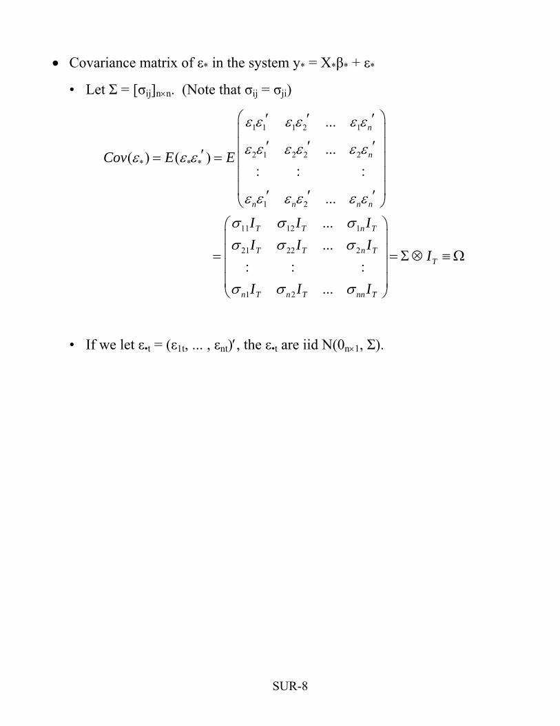
• Covariance matrix of ε* in the system y* = X*β* + ε*
• Let Σ = [σij]n×n. (Note that σij = σji)
SUR-8
Σ⊗ ≡ Ω
1 1 1 2 1
2 1 2 2 2* * *
1 2
11 12 1
21 22 2
1 2
...
...( ) ( ): : :
...
...
...: : :
...
n
n
n n n n
T T n T
T T n TT
n T n T nn T
Cov E E
I I II I I
I
I I I
ε ε ε ε ε ε
ε ε ε ε ε εε ε ε
ε ε ε ε ε ε
σ σ σσ σ σ
σ σ σ
⎛ ⎞′ ′ ′⎜ ⎟
′ ′ ′⎜ ⎟′= = ⎜ ⎟⎜ ⎟⎜ ⎟′ ′ ′⎝ ⎠
⎛ ⎞⎜ ⎟⎜ ⎟= =⎜ ⎟⎜ ⎟⎝ ⎠
• If we let ε•t = (ε1t, ... , εnt)′, the ε•t are iid N(0n×1, Σ).
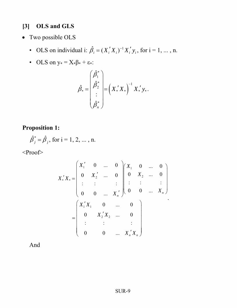
[3] OLS and GLS
• Two possible OLS
SUR-9
i • OLS on individual i: 1ˆ ( )i i i iX X X yβ −′ ′= , for i = 1, ... , n.
• OLS on y* = X*β* + ε*:
( )*1
* 12
* * *
*
ˆ
ˆˆ:ˆ
n
X X X y
β
ββ
β
−
⎛ ⎞⎜ ⎟⎜ ⎟
* *′ ′= =⎜ ⎟
⎜ ⎟⎜ ⎟⎝ ⎠
.
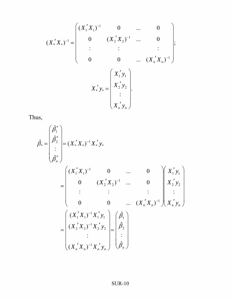
Proposition 1: *ˆ ˆj jβ β= , for i = 1, 2, ... , n.
<Proof>
.
1 1
22* *
1 1
2 2
0 ... 0 0 ... 00 ...0 ... 0: : :: : :0 0 ...0 0 ...
0 ... 0
0 ... 0: : :
0 0 ...
nn
n n
X XXXX X
XX
X X
X X
X X
⎛ ⎞′ ⎛ ⎞⎜ ⎟⎜ ⎟⎜ ⎟′ ⎜ ⎟′ = ⎜ ⎟⎜ ⎟⎜ ⎟⎜ ⎟⎜ ⎟⎜ ⎟⎝ ⎠′⎝ ⎠⎛ ⎞′⎜ ⎟⎜ ⎟′
= ⎜ ⎟⎜ ⎟⎜ ⎟⎜ ⎟′⎝ ⎠
0
And
SUR-10
)
;
11 1
11 2 2
* *
1
( ) 0 ... 0
0 ( ) ... 0( ): : :
0 0 ... ( n n
X X
X XX X
X X
−
−−
−
⎛ ⎞′⎜ ⎟
′⎜ ⎟′ = ⎜ ⎟⎜ ⎟⎜ ⎟′⎝ ⎠
1 1
2 2* *
:
n n
X y
X yX y
X y
⎛ ⎞′⎜ ⎟
′⎜ ⎟′ = ⎜ ⎟⎜ ⎟⎜ ⎟′⎝ ⎠
.
Thus,
*1
*12
* * * * *
*
11 1 1 1
12 2 2 2
1
11 1 1 1 1
12 2 2 2
1
ˆ
ˆˆ ( ):ˆ
( ) 0 ... 0
0 ( ) ... 0: : :
0 0 ... ( )
ˆ( )ˆ( )
:
( )
n
n n n n
n n n n
X X X y
X X X y
X X X y
X X X y
X X X y
X X X y
X X X y
β
ββ
β
β
β
−
−
−
−
−
−
−
⎛ ⎞⎜ ⎟⎜ ⎟ ′ ′= =⎜ ⎟⎜ ⎟⎜ ⎟⎝ ⎠
⎛ ⎞′ ′⎜ ⎟
:
⎛ ⎞⎜ ⎟
′ ′⎜ ⎟= ⎜ ⎟⎜ ⎟⎜ ⎟
⎜ ⎟⎜ ⎟⎜ ⎟⎜ ⎟′ ′⎝ ⎠
⎛ ⎞′ ′⎜ ⎟
′ ′⎜ ⎟= =⎜ ⎟⎜ ⎟⎜ ⎟′ ′⎝ ⎠
2
:ˆnβ
⎛ ⎞⎜ ⎟⎜ ⎟⎜ ⎟⎜ ⎟⎜ ⎟⎝ ⎠
⎝ ⎠
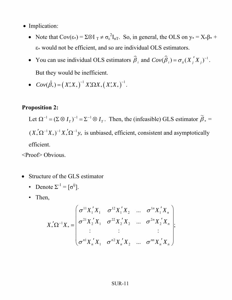
• Implication:
• Note that Cov(ε*) = Σ⊗I T ≠ σε2InT. So, in general, the OLS on y* = X*β* +
ε* would not be efficient, and so are individual OLS estimators.
• You can use individual OLS estimators iβ and 1( ) ( )ii j jiCov X Xβ σ −′= .
But they would be inefficient.
• ( ) ( )1 1* * * * * * *
ˆ( )Cov X X X X X Xβ − −′ ′ ′= Ω .
Proposition 2:
Let 1 1 1( )T TI I− − −Ω = Σ⊗ = Σ ⊗ . Then, the (infeasible) GLS estimator *β =
1 1 1* * *( )X X X *y− − −′ ′Ω Ω is unbiased, efficient, consistent and asymptotically
efficient.
<Proof> Obvious.
• Structure of the GLS estimator
• Denote Σ-1 = [σij].
• Then,
;
11 12 11 1 1 2 1
21 22 21 2 1 2 2 2
* *
1 21 2
...
...: : :
...
nn
nn
n n nnn n n
X X X X X X
X X X X X XX X
X X X X X X
σ σ σ
σ σ σ
σ σ σ
−
⎛ ⎞′ ′⎜ ⎟
′ ′⎜ ⎟′Ω = ⎜ ⎟⎜ ⎟⎜ ⎟′ ′⎝ ⎠n
′
′
′
SUR-11
11 1
21 1 2
* *
1
:
n jj j
n jj j
n njj n j
X y
X yX y
X y
σ
σ
σ
=
− =
=
⎛ ⎞′Σ⎜ ⎟
′⎜ ⎟Σ′Ω = ⎜ ⎟⎜ ⎟⎜ ⎟⎜ ⎟′Σ⎝ ⎠
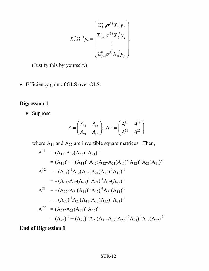
.
(Justify this by yourself.)
• Efficiency gain of GLS over OLS:
Digression 1
• Suppose
11 12
21 22
A AA
A A⎛ ⎞
= ⎜ ⎟⎝ ⎠
; 11 12
121 22
A AA
A A− ⎛ ⎞= ⎜ ⎟⎝ ⎠
where A11 and A22 are invertible square matrices. Then,
A11 = (A11-A12(A22)-1A21)-1
= (A11)-1 + (A11)-1A12(A22-A21(A11)-1A12)-1A21(A11)-1
A12 = - (A11)-1A12(A22-A21(A11)-1A12)-1
= - (A11-A12(A22)-1A21)-1A12(A22)-1
A21 = - (A22-A21(A11)-1A12)-1A21(A11)-1
= - (A22)-1A21(A11-A12(A22)-1A21)-1
A22 = (A22-A21(A11)-1A12)-1
= (A22)-1 + (A22)-1A21(A11-A12(A22)-1A21)-1A12(A22)-1
End of Digression 1
SUR-12
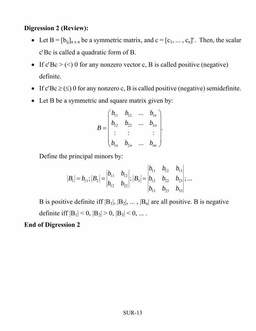
Digression 2 (Review):
• Let B = [bij]n x n be a symmetric matrix, and c = [c1, ... , cn]′. Then, the scalar
c′Bc is called a quadratic form of B.
• If c′Bc > (<) 0 for any nonzero vector c, B is called positive (negative)
definite.
• If c′Bc ≥ (≤) 0 for any nonzero c, B is called positive (negative) semidefinite.
• Let B be a symmetric and square matrix given by:
.
11 12 1
12 22 2
1 2
...
...: : :
...
n
n
n n nn
b b bb b b
B
b b b
⎛ ⎞⎜ ⎟⎜ ⎟=⎜ ⎟⎜ ⎟⎝ ⎠
Define the principal minors by:
11 12 13
11 121 11 2 3 12 22 23
12 2213 23 33
; ;b b b
b bB b B B b b b
b bb b b
= = = ; ...
B is positive definite iff |B1|, |B2|, ... , |Bn| are all positive. B is negative
definite iff |B1| < 0, |B2| > 0, |B3| < 0, ... .
End of Digression 2
SUR-13
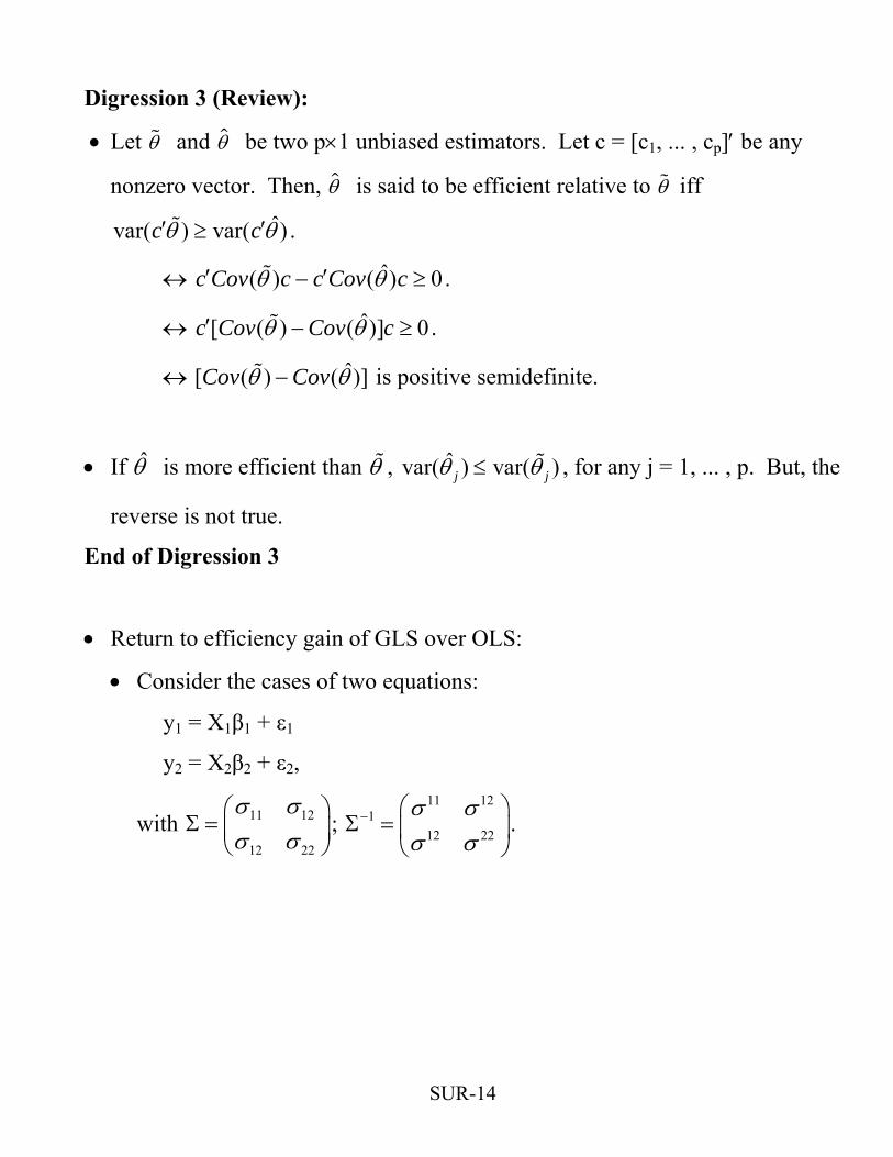
Digression 3 (Review):
• Let θ and θ be two p×1 unbiased estimators. Let c = [c1, ... , cp]′ be any
nonzero vector. Then, θ is said to be efficient relative to θ iff
ˆvar( ) var( )c cθ θ′ ′≥ .
↔ . ˆ( ) ( ) 0c Cov c c Cov cθ θ′ ′− ≥
↔ . ˆ[ ( ) ( )]c Cov Cov cθ θ′ − ≥ 0
)]↔ ˆ[ ( ) (Cov Covθ θ− is positive semidefinite.
• If θ is more efficient than θ , ˆvar( ) var( )j jθ θ≤ , for any j = 1, ... , p. But, the
reverse is not true.
End of Digression 3
• Return to efficiency gain of GLS over OLS:
• Consider the cases of two equations:
y1 = X1β1 + ε1
y2 = X2β2 + ε2,
with 11 12
12 22
σ σσ σ⎛ ⎞
Σ = ⎜ ⎟⎝ ⎠
; . 11 12
112 22
σ σσ σ
− ⎛ ⎞Σ = ⎜ ⎟
⎝ ⎠
SUR-14
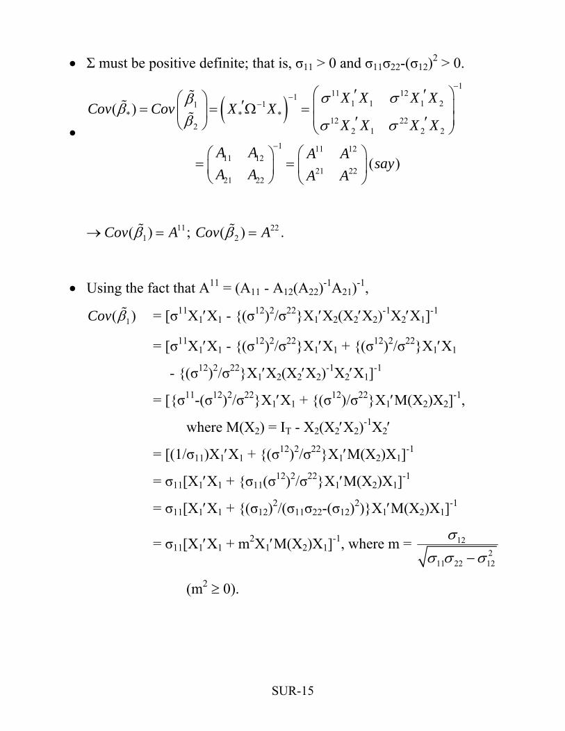
• Σ must be positive definite; that is, σ11 > 0 and σ11σ22-(σ12)2 > 0.
• ( )
111 121
1 1 1 211* * *
12 222 2 1 2 2
1 11 1211 12
21 2221 22
( )
( )
X X X XCov Cov X X
X X X X
A A A Asay
A A A A
σ σββ
β σ σ
−−
−
−
⎛ ⎞′ ′⎛ ⎞ ′ ⎜ ⎟= = Ω =⎜ ⎟ ⎜ ⎟′ ′⎝ ⎠ ⎝ ⎠
⎛ ⎞⎛ ⎞= = ⎜ ⎟⎜ ⎟⎝ ⎠ ⎝ ⎠
→ ; . 111( )Cov Aβ = 22
2( )Cov Aβ =
• Using the fact that A11 = (A11 - A12(A22)-1A21)-1,
SUR-15
)1(Cov β = [σ11X1′X1 - (σ12)2/σ22X1′X2(X2′X2)-1X2′X1]-1
= [σ11X1′X1 - (σ12)2/σ22X1′X1 + (σ12)2/σ22X1′X1
- (σ12)2/σ22X1′X2(X2′X2)-1X2′X1]-1
= [σ11-(σ12)2/σ22X1′X1 + (σ12)/σ22X1′M(X2)X2]-1,
where M(X2) = IT - X2(X2′X2)-1X2′
= [(1/σ11)X1′X1 + (σ12)2/σ22X1′M(X2)X1]-1
= σ11[X1′X1 + σ11(σ12)2/σ22X1′M(X2)X1]-1
= σ11[X1′X1 + (σ12)2/(σ11σ22-(σ12)2)X1′M(X2)X1]-1
= σ11[X1′X1 + m2X1′M(X2)X1]-1, where m = 122
11 22 12
σσ σ σ−
(m2 ≥ 0).
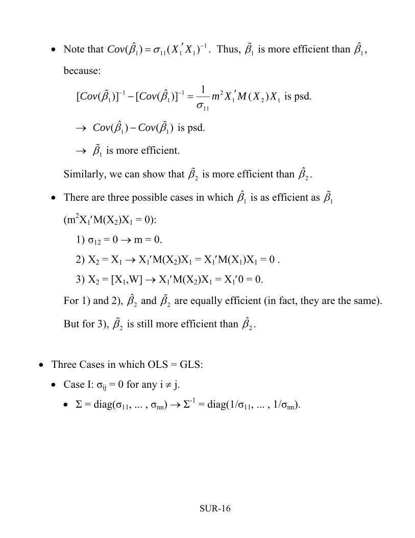
• Note that 11 11 1 1
ˆ( ) ( )Cov X Xβ σ −′= . Thus, 1β is more efficient than 1β ,
because:
1 1 21 1 1
11
1ˆ[ ( )] [ ( )] ( )Cov Cov m X M X Xβ βσ
− − ′− = 2 1
)
is psd.
→ 1 1ˆ( ) (Cov Covβ β− is psd.
→ 1β is more efficient.
Similarly, we can show that 2β is more efficient than 2β .
• There are three possible cases in which 1β is as efficient as 1β
(m2X1′M(X2)X1 = 0):
1) σ12 = 0 → m = 0.
2) X2 = X1 → X1′M(X2)X1 = X1′M(X1)X1 = 0 .
3) X2 = [X1,W] → X1′M(X2)X1 = X1′0 = 0.
For 1) and 2), 2β and 2β are equally efficient (in fact, they are the same).
But for 3), 2β is still more efficient than 2β .
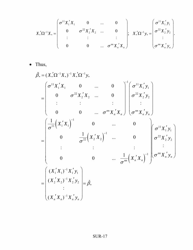
• Three Cases in which OLS = GLS:
• Case I: σij = 0 for any i ≠ j.
• Σ = diag(σ11, ... , σnn) → Σ-1 = diag(1/σ11, ... , 1/σnn).
SUR-16
SUR-17
: : :
0 0 ... nnn n
X X
X XX X
X X
σ
σ
σ
−
⎛ ⎞′⎜ ⎟⎜ ⎟′′Ω = ⎜ ⎟⎜ ⎟⎜ ⎟′⎝ ⎠
111 1
221 2 2
* *:
nnn n
X y
X yX y
X y
σ
σ
σ
−
⎛ ⎞′111 1
221 2 2
* *
0 ... 0
0 ... 0 ; ⎜ ⎟⎜ ⎟′′Ω = ⎜ ⎟⎜ ⎟⎜ ⎟′⎝ ⎠
.
• Thus,
( )( )
( )
1 1 1* * * * *
111 11
1 1 1 1
22 222 2 2 2
1
1 111 111
1
2 222
1
( )
0 ... 0
0 ... 0: : : :
0 0 ...
1 0 ... 0
10 ... 0
: : :10 0 ...
nn nnn n n n
n nnn
X X X y
X X X y
X X X y
X X X y
X XX
X X
X X
β
σ σ
σ σ
σ σ
σ σ
σ
σ
− − −
−
−
−
−
′ ′= Ω Ω
⎛ ⎞ ⎛′ ′⎜ ⎟ ⎜
′ ′⎜ ⎟ ⎜= ⎜ ⎟ ⎜⎜ ⎟ ⎜⎜ ⎟ ⎜′ ′⎝ ⎠ ⎝⎛ ⎞′⎜ ⎟
⎞⎟⎟⎟⎟⎟⎠
′⎜ ⎟⎜ ⎟′
= ⎜ ⎟⎜ ⎟⎜ ⎟⎜ ⎟′⎜ ⎟⎝ ⎠
1
222 2
11 1 1 1
12 2 2 2
*
1
:
( )
( ) ˆ:
( )
nnn n
n n n n
y
X y
X y
X X X y
X X X y
X X X y
σ
σ
β
−
−
−
⎛ ⎞⎜ ⎟
′⎜ ⎟⎜ ⎟⎜ ⎟⎜ ⎟′⎝ ⎠
⎛ ⎞′ ′⎜ ⎟
′ ′⎜ ⎟= =⎜ ⎟⎜ ⎟⎜ ⎟′ ′⎝ ⎠

• Case II: X1 = X2 = ... = X.
• This is the case where the values of regressors are the same for all
equations.
SUR-18
X= ⊗ *
0 ... 0 1 0 ... 00 ... 0 0 1 ... 0: : : : : :0 0 ... 0 0 ... 1
n
X X X XX X X X
X I
X X X X
⎛ ⎞ ⎛ ⎞⎜ ⎟ ⎜ ⎟⎜ ⎟ ⎜ ⎟= =⎜ ⎟ ⎜ ⎟⎜ ⎟ ⎜ ⎟⎝ ⎠ ⎝ ⎠
• Then,
*β = [X*′Ω-1X*]-1X*′Ω-1y*
= [(In⊗X)′(Σ-1⊗IT)(In⊗X)]-1(In⊗X)′(Σ-1⊗IT)y*
= [Σ-1⊗X′X]-1(Σ-1⊗X′)y*
= (Σ⊗(X′X)-1)(Σ-1⊗X′)y*
= (In⊗(X′X)-1X′)y*
=
111 1
112 2
11
( )( ) 0 ... 0( )0 ( ) ... 0
: :: : :( )0 0 ... ( ) n n
y X X X yX X Xy X X X yX X X
y X X X yX X X
−−
−−
−−
′ ′′ ′ ⎛ ⎞⎛ ⎞⎛ ⎞⎜ ⎟⎜ ⎟⎜ ⎟ ′ ′′ ′ ⎜ ⎟⎜ ⎟⎜ ⎟ =⎜ ⎟⎜ ⎟⎜ ⎟⎜ ⎟⎜ ⎟⎜ ⎟ ⎜ ⎟′ ′′ ′ ⎝ ⎠⎝ ⎠ ⎝ ⎠
= *β
• Case III: X1, X2, ... , Xm ⊂ Xm+1, Xm+2, ... , Xn
i iβ β= for i = 1, 2, ... , m. But jβ are still more efficient than ˆjβ for j =
m+1, ... , n.
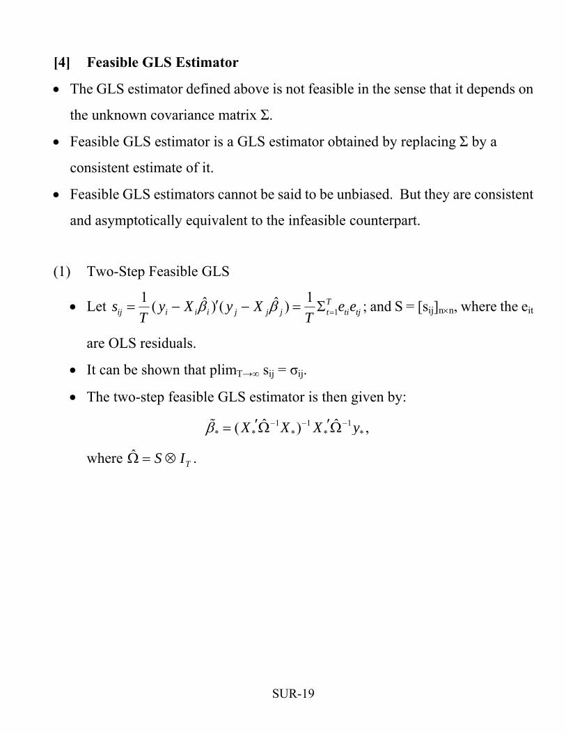
[4] Feasible GLS Estimator
• The GLS estimator defined above is not feasible in the sense that it depends on
the unknown covariance matrix Σ.
• Feasible GLS estimator is a GLS estimator obtained by replacing Σ by a
consistent estimate of it.
• Feasible GLS estimators cannot be said to be unbiased. But they are consistent
and asymptotically equivalent to the infeasible counterpart.
(1) Two-Step Feasible GLS
• Let 11 ˆ ˆ( ) ( ) T
ij i i i j j j t ti tj1s y X y X e e
T Tβ β =′= − − = Σ ; and S = [sij]n×n, where the eit
are OLS residuals.
• It can be shown that plimT→∞ sij = σij.
• The two-step feasible GLS estimator is then given by:
1 1 1* * * *
ˆ ˆ( )X X X *yβ − − −′ ′= Ω Ω ,
where . ˆTS IΩ = ⊗
SUR-19
Digression:
• As long as T is large, sij is a consistent estimator.
• If n is small, as long as T is large, Σ can be said that it is a consistent
estimator of Σ .
• If both T and n are large, is Σ consistent?
• Not necessarily.
• If n > T, it can be shown that Σ is psd, but not pd. That is, Σ is not
invertible.
• Not invertible cannot be a consistent estimator of Σ . Σ
• Important research agenda!
End of Digression
(2) Iterative Feasible GLS.
• Using the two-step GLS estimator, recompute S.
• Using this recomputed S, recompute the feasible GLS estimator.
• Repeat this procedure, until the value of FGLS does not change.
(3) Facts:
• The two-step and iterative feasible GLS are asymptotically equivalent to the
MLE under the normality assumption about the ε’s.
• In fact, iterative feasible GLS = MLE, numerically.
SUR-20
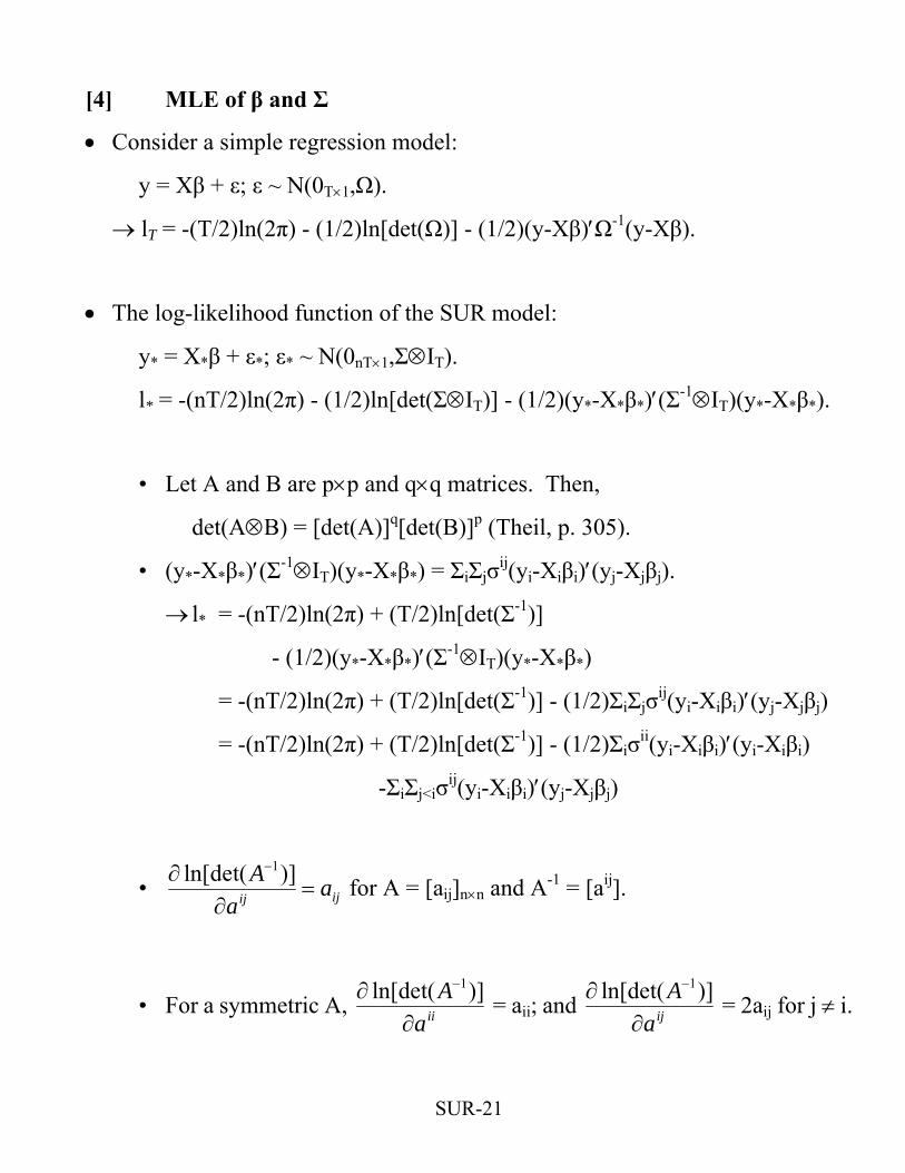
[4] MLE of β and Σ
• Consider a simple regression model:
y = Xβ + ε; ε ~ N(0T×1,Ω).
→ lT = -(T/2)ln(2π) - (1/2)ln[det(Ω)] - (1/2)(y-Xβ)′Ω-1(y-Xβ).
• The log-likelihood function of the SUR model:
y* = X*β + ε*; ε* ~ N(0nT×1,Σ⊗IT).
l* = -(nT/2)ln(2π) - (1/2)ln[det(Σ⊗IT)] - (1/2)(y*-X*β*)′(Σ-1⊗IT)(y*-X*β*).
• Let A and B are p×p and q×q matrices. Then,
det(A⊗B) = [det(A)]q[det(B)]p (Theil, p. 305).
• (y*-X*β*)′(Σ-1⊗IT)(y*-X*β*) = ΣiΣjσij(yi-Xiβi)′(yj-Xjβj).
→ l* = -(nT/2)ln(2π) + (T/2)ln[det(Σ-1)]
- (1/2)(y*-X*β*)′(Σ-1⊗IT)(y*-X*β*)
= -(nT/2)ln(2π) + (T/2)ln[det(Σ-1)] - (1/2)ΣiΣjσij(yi-Xiβi)′(yj-Xjβj)
= -(nT/2)ln(2π) + (T/2)ln[det(Σ-1)] - (1/2)Σiσii(yi-Xiβi)′(yi-Xiβi)
-ΣiΣj<iσij(yi-Xiβi)′(yj-Xjβj)
• 1ln[det( )]
ijijA a
a
−∂=
∂ for A = [aij]n×n and A-1 = [aij].
• For a symmetric A, 1ln[det( )]
iiA
a
−∂∂
= aii; and 1ln[det( )]
ijA
a
−∂∂
= 2aij for j ≠ i.
SUR-21
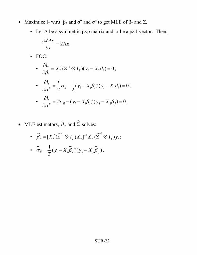
• Maximize l* w.r.t. β* and σii and σij to get MLE of β* and Σ.
• Let A be a symmetric p×p matrix and; x be a p×1 vector. Then,
x Axx′∂∂
= 2Ax.
• FOC:
• 1** * *
*
( )( )Tl X I y X ββ
−∂ ′= Σ ⊗ − =∂ * 0 ;
• * 1 ( ) ( )2 2ii i i i i i iii
l T y X y Xσ β 0βσ∂ ′= − − − =∂
;
• * ( ) ( )ij i i i j j jijl T y X y Xσ β β 0σ∂ ′= − − − =∂
.
• MLE estimators, *β and solves: Σ
• 1 11
* * ** [ ( ) ] ( )T TX I X X I *yβ− −−′ ′= Σ ⊗ Σ ⊗ ;
• 1 ( ) (ij i i j ji jy X y XT
)σ β β′= − − .
SUR-22
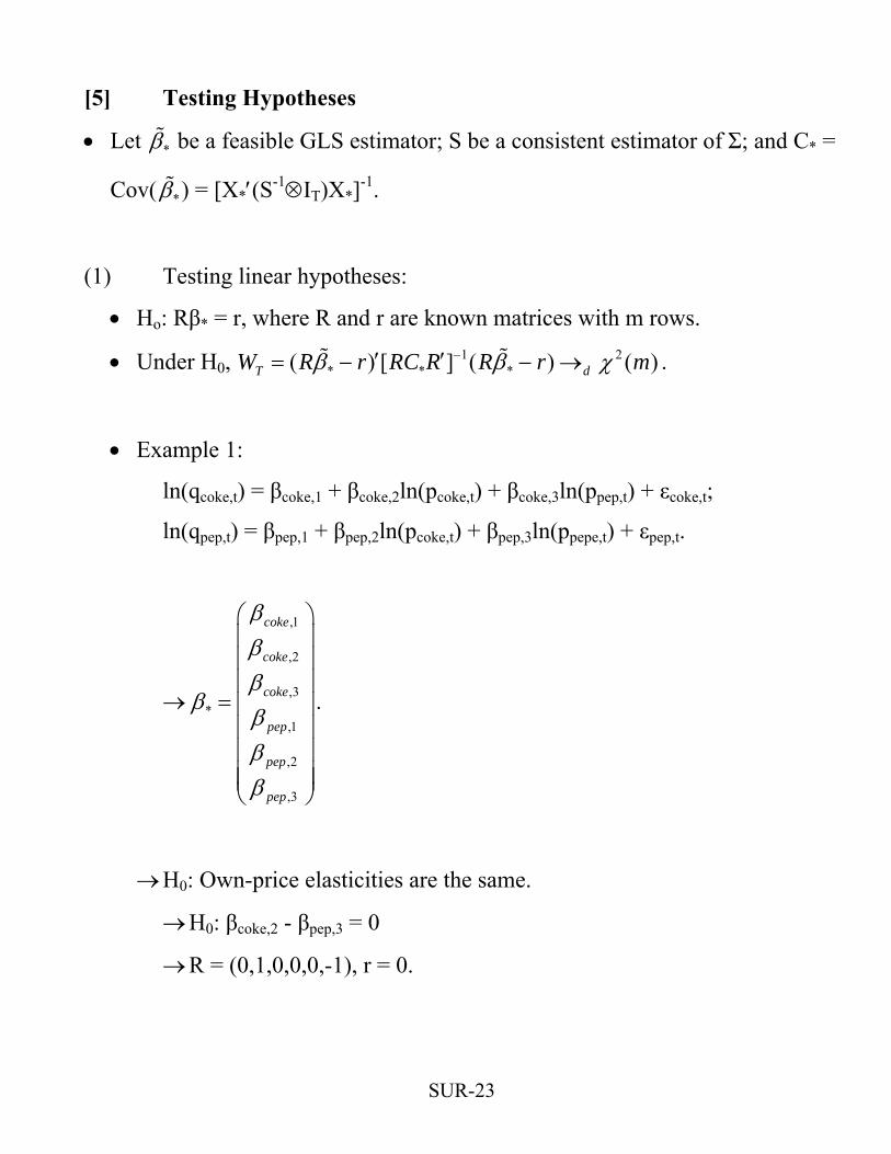
[5] Testing Hypotheses
• Let *β be a feasible GLS estimator; S be a consistent estimator of Σ; and C* =
Cov( *β ) = [X*′(S-1⊗IT)X*]-1.
(1) Testing linear hypotheses:
• Ho: Rβ* = r, where R and r are known matrices with m rows.
• Under H0, . 1 2* * *( ) [ ] ( ) (T dW R r RC R R r mβ β−′ ′= − − → )χ
• Example 1:
ln(qcoke,t) = βcoke,1 + βcoke,2ln(pcoke,t) + βcoke,3ln(ppep,t) + εcoke,t;
ln(qpep,t) = βpep,1 + βpep,2ln(pcoke,t) + βpep,3ln(ppepe,t) + εpep,t.
→
,1
,2
,3*
,1
,2
,3
coke
coke
coke
pep
pep
pep
βββ
ββββ
⎛ ⎞⎜ ⎟⎜ ⎟⎜ ⎟
= ⎜ ⎟⎜ ⎟⎜ ⎟⎜ ⎟⎜ ⎟⎝ ⎠
.
→ H0: Own-price elasticities are the same.
→ H0: βcoke,2 - βpep,3 = 0
→ R = (0,1,0,0,0,-1), r = 0.
SUR-23
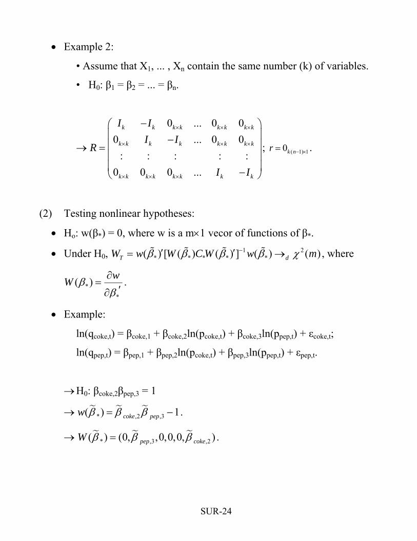
• Example 2:
• Assume that X1, ... , Xn contain the same number (k) of variables.
• H0: β1 = β2 = ... = βn.
→
0 ... 0 00 ... 0 0
: : : : :0 0 0 ...
k k k k k k k k
k k k k k k k k
k k k k k k k k
I II I
R
I I
× × ×
×× ×
× × ×
−⎛ ⎞⎜ ⎟−⎜ ⎟=⎜ ⎟⎜ ⎟−⎝ ⎠
( 1) 10k nr − ×; = .
(2) Testing nonlinear hypotheses:
• Ho: w(β*) = 0, where w is a m×1 vecor of functions of β*.
• Under H0, , where 1 2* * * * *( ) [ ( ) ( ) ] ( ) (T dW w W C W w mβ β β β χ−′ ′= → )
*
*
( ) wW ββ∂
=′∂.
• Example:
ln(qcoke,t) = βcoke,1 + βcoke,2ln(pcoke,t) + βcoke,3ln(ppep,t) + εcoke,t;
ln(qpep,t) = βpep,1 + βpep,2ln(pcoke,t) + βpep,3ln(ppep,t) + εpep,t.
→ H0: βcoke,2βpep,3 = 1
→ . * ,2 ,3( ) coke pepw β β β= −1
→ * ,3( ) (0, ,0,0,0, )pep cokeW β β β= ,2 .
SUR-24
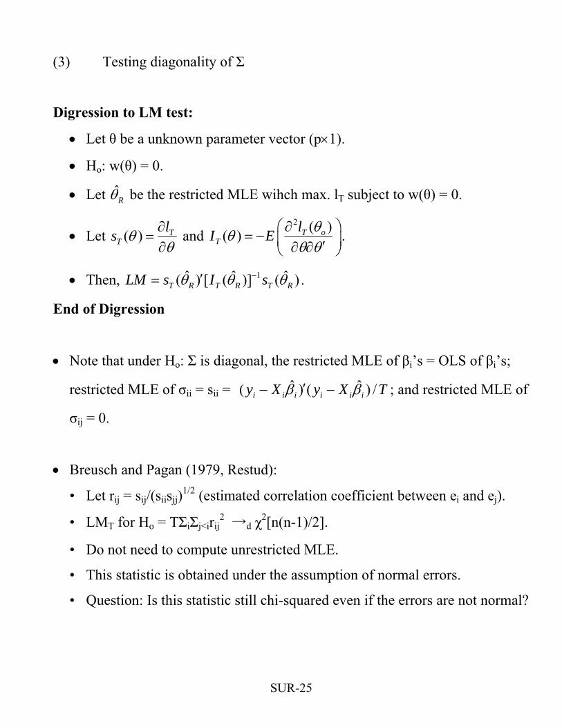
(3) Testing diagonality of Σ
Digression to LM test:
• Let θ be a unknown parameter vector (p×1).
• Ho: w(θ) = 0.
• Let Rθ be the restricted MLE wihch max. lT subject to w(θ) = 0.
• Let ( ) TT
ls θθ∂
=∂
and 2 ( )( ) T o
TlI E θθθ θ
⎛ ⎞∂= − ⎜ ⎟′∂ ∂⎝ ⎠
.
• Then, 1ˆ ˆ( ) [ ( )] ( )T R T R T RLM s I s ˆθ θ θ−′= .
End of Digression
• Note that under Ho: Σ is diagonal, the restricted MLE of βi’s = OLS of βi’s;
restricted MLE of σii = sii = ; and restricted MLE of
σ
ˆ ˆ( ) (i i i i i iy X y X Tβ β′− − ) /
ij = 0.
• Breusch and Pagan (1979, Restud):
• Let rij = sij/(siisjj)1/2 (estimated correlation coefficient between ei and ej).
• LMT for Ho = TΣiΣj<irij2 →d χ2[n(n-1)/2].
• Do not need to compute unrestricted MLE.
• This statistic is obtained under the assumption of normal errors.
• Question: Is this statistic still chi-squared even if the errors are not normal?
SUR-25
SUR-26
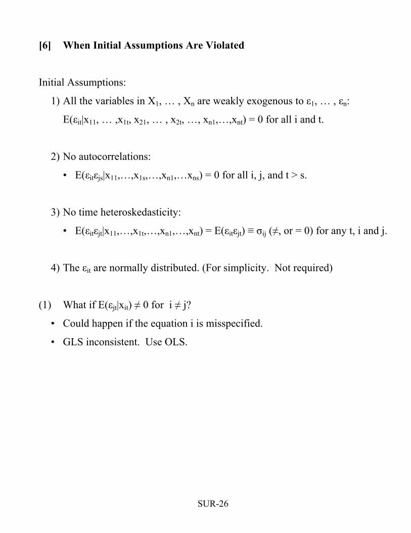
[6] When Initial Assumptions Are Violated
Initial Assumptions:
1) All the variables in X1, … , Xn are weakly exogenous to ε1, … , εn:
E(εit|x11, … ,x1t, x21, … , x2t, …, xn1,…,xnt) = 0 for all i and t.
2) No autocorrelations:
• E(εitεjs|x11,…,x1s,…,xn1,…xns) = 0 for all i, j, and t > s.
3) No time heteroskedasticity:
• E(εitεjt|x11,…,x1t,…,xn1,…,xnt) = E(εitεjt) ≡ σij (≠, or = 0) for any t, i and j.
4) The εit are normally distributed. (For simplicity. Not required)
(1) What if E(εjt|xit) ≠ 0 for i ≠ j?
• Could happen if the equation i is misspecified.
• GLS inconsistent. Use OLS.
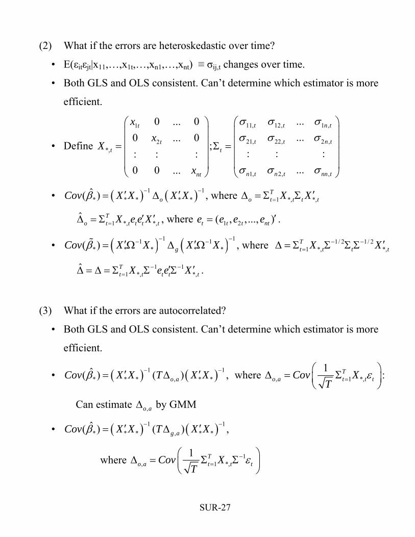
(2) What if the errors are heteroskedastic over time?
• E(εitεjt|x11,…,x1t,…,xn1,…,xnt) ≡ σij,t changes over time.
• Both GLS and OLS consistent. Can’t determine which estimator is more
efficient.
SUR-27
: : :0 0 ...
t
tt
nt
xx
• Define X
1
2*,
0 ... 00 ... 0
x
⎛ ⎞⎜ ⎟⎜ ⎟=⎜ ⎟⎜ ⎟⎝ ⎠
11, 12, 1 ,
21, 22, 2 ,
1, 2, ,
...
...: : :
...
t t n t
t t n tt
n t n t nn t
σ σ σσ σ σ
σ σ σ
⎛ ⎞⎜ ⎟⎜ ⎟Σ =⎜ ⎟⎜ ⎟⎝ ⎠
) t
t
;
• , where ( ) (1 1* * * * *
ˆ( ) oCov X X X Xβ − −′ ′= Δ 1 *, *,T
o t t tX X= ′Δ = Σ Σ
, where 1 *, *,ˆ T
o t t t tX e e X= ′ ′Δ = Σ 1 2( , ,..., )t t t nte e e e ′= .
• ( ) ( )1 11 1* * * * *( ) gCov X X X Xβ
− −−′ ′= Ω Δ Ω−t, where 1/ 2 1/ 2
1 *, *,Tt t tX X− −= ′Δ = Σ Σ Σ Σ
1 11 *, *,
ˆ Tt t t tX e e X− −= t′ ′Δ = Δ = Σ Σ Σ .
(3) What if the errors are autocorrelated?
• Both GLS and OLS consistent. Can’t determine which estimator is more
efficient.
• ( ) ( )1 1* * * , * *
ˆ( ) ( )o aCov X X T X Xβ − −′ ′= Δ , where , 11 T
o a t t tCov XT *, ε=
⎛ ⎞Δ = Σ⎜ ⎟⎝ ⎠
:
Can estimate by GMM ,o aΔ
• ( ) ( )1 1* * * , * *
ˆ( ) ( )g aCov X X T X Xβ − −′ ′= Δ ,
where 1, 1 *
1 To a t t tCov X
T , ε−=
⎛ ⎞Δ = Σ Σ⎜ ⎟⎝ ⎠
SUR-28
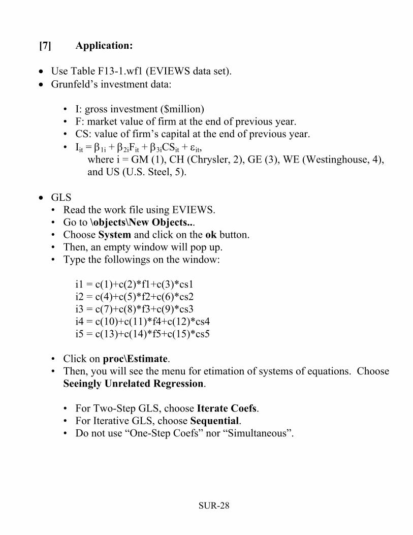
[7] Application: • Use Table F13-1.wf1 (EVIEWS data set). • Grunfeld’s investment data: • I: gross investment ($million) • F: market value of firm at the end of previous year. • CS: value of firm’s capital at the end of previous year. • Iit = β1i + β2iFit + β3iCSit + εit,
where i = GM (1), CH (Chrysler, 2), GE (3), WE (Westinghouse, 4), and US (U.S. Steel, 5).
• GLS • Read the work file using EVIEWS. • Go to \objects\New Objects... • Choose System and click on the ok button. • Then, an empty window will pop up. • Type the followings on the window: i1 = c(1)+c(2)*f1+c(3)*cs1 i2 = c(4)+c(5)*f2+c(6)*cs2 i3 = c(7)+c(8)*f3+c(9)*cs3 i4 = c(10)+c(11)*f4+c(12)*cs4 i5 = c(13)+c(14)*f5+c(15)*cs5 • Click on proc\Estimate.
• Then, you will see the menu for etimation of systems of equations. Choose Seeingly Unrelated Regression.
• For Two-Step GLS, choose Iterate Coefs. • For Iterative GLS, choose Sequential. • Do not use “One-Step Coefs” nor “Simultaneous”.
SUR-29
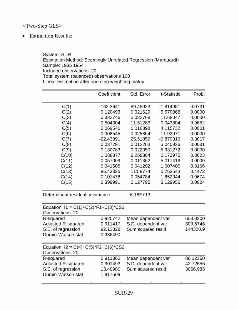
<Two-Step GLS>
• Estimation Results:
System: SUR Estimation Method: Seemingly Unrelated Regression (Marquardt) Sample: 1935 1954 Included observations: 20 Total system (balanced) observations 100 Linear estimation after one-step weighting matrix
Coefficient Std. Error t-Statistic Prob.
C(1) -162.3641 89.45923 -1.814951 0.0731C(2) 0.120493 0.021629 5.570868 0.0000C(3) 0.382746 0.032768 11.68047 0.0000C(4) 0.504304 11.51283 0.043804 0.9652C(5) 0.069546 0.016898 4.115732 0.0001C(6) 0.308545 0.025864 11.92971 0.0000C(7) -22.43891 25.51859 -0.879316 0.3817C(8) 0.037291 0.012263 3.040936 0.0031C(9) 0.130783 0.022050 5.931272 0.0000C(10) 1.088877 6.258804 0.173975 0.8623C(11) 0.057009 0.011362 5.017416 0.0000C(12) 0.041506 0.041202 1.007400 0.3166C(13) 85.42325 111.8774 0.763543 0.4473C(14) 0.101478 0.054784 1.852344 0.0674C(15) 0.399991 0.127795 3.129956 0.0024
Determinant residual covariance 6.18E+13
Equation: I1 = C(1)+C(2)*F1+C(3)*CS1 Observations: 20 R-squared 0.920742 Mean dependent var 608.0200Adjusted R-squared 0.911417 S.D. dependent var 309.5746S.E. of regression 92.13828 Sum squared resid 144320.9Durbin-Watson stat 0.936490
Equation: I2 = C(4)+C(5)*F2+C(6)*CS2 Observations: 20 R-squared 0.911862 Mean dependent var 86.12350Adjusted R-squared 0.901493 S.D. dependent var 42.72556S.E. of regression 13.40980 Sum squared resid 3056.985Durbin-Watson stat 1.917509
SUR-30
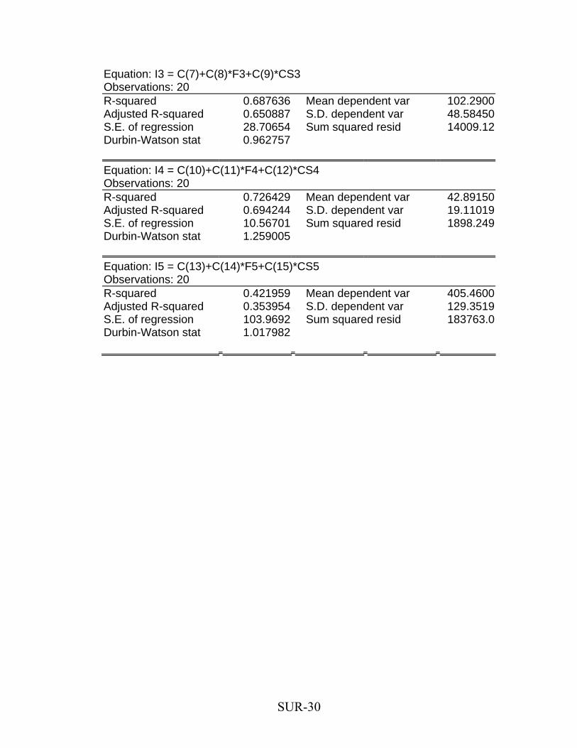
Equation: I3 = C(7)+C(8)*F3+C(9)*CS3 Observations: 20 R-squared 0.687636 Mean dependent var 102.2900Adjusted R-squared 0.650887 S.D. dependent var 48.58450S.E. of regression 28.70654 Sum squared resid 14009.12Durbin-Watson stat 0.962757
Equation: I4 = C(10)+C(11)*F4+C(12)*CS4 Observations: 20 R-squared 0.726429 Mean dependent var 42.89150Adjusted R-squared 0.694244 S.D. dependent var 19.11019S.E. of regression 10.56701 Sum squared resid 1898.249Durbin-Watson stat 1.259005
Equation: I5 = C(13)+C(14)*F5+C(15)*CS5 Observations: 20 R-squared 0.421959 Mean dependent var 405.4600Adjusted R-squared 0.353954 S.D. dependent var 129.3519S.E. of regression 103.9692 Sum squared resid 183763.0Durbin-Watson stat 1.017982
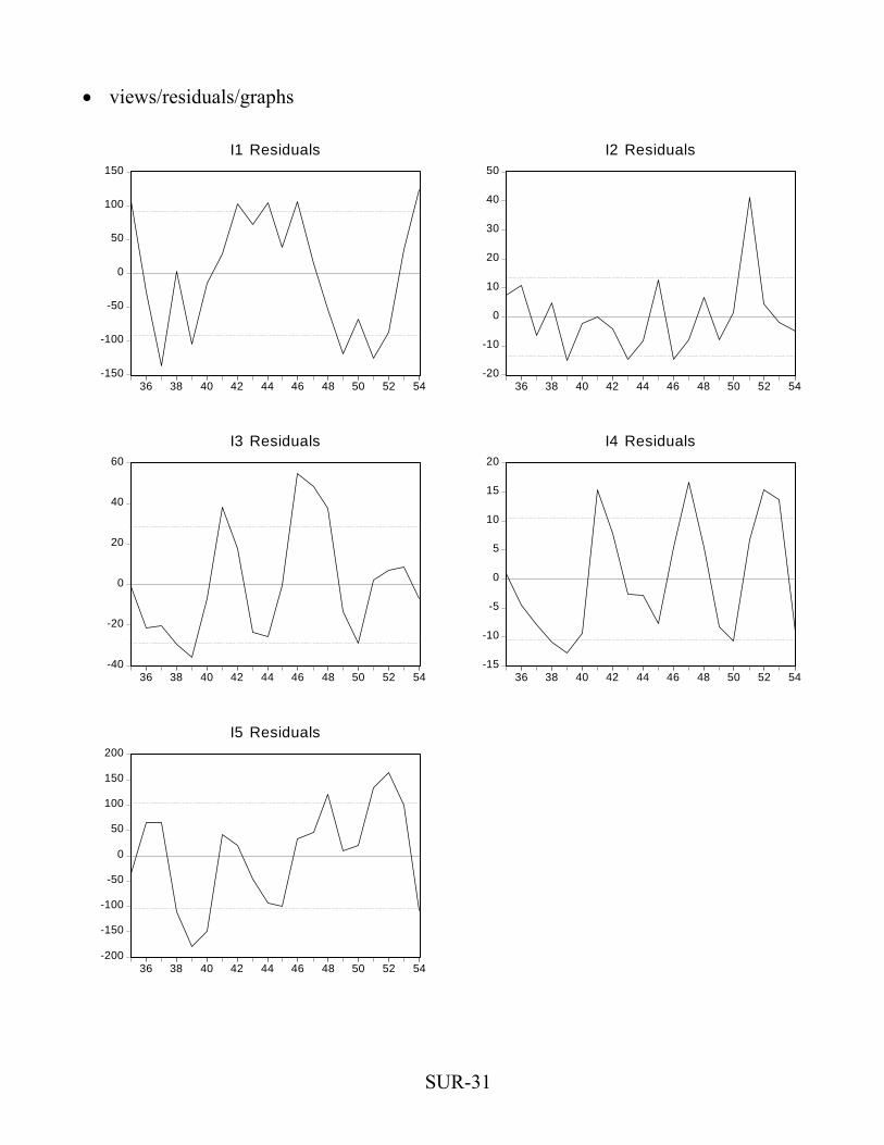
• views/residuals/graphs
-150
-100
-50
0
50
100
150
36 38 40 42 44 46 48 50 52 54
I1 Residuals
-20
-10
0
10
20
30
40
50
36 38 40 42 44 46 48 50 52 54
I2 Residuals
-40
-20
0
20
40
60
36 38 40 42 44 46 48 50 52 54
I3 Residuals
-15
-10
-5
0
5
10
15
20
36 38 40 42 44 46 48 50 52 54
I4 Residuals
-200
-150
-100
-50
0
50
100
150
200
36 38 40 42 44 46 48 50 52 54
I5 Residuals
SUR-31
SUR-32
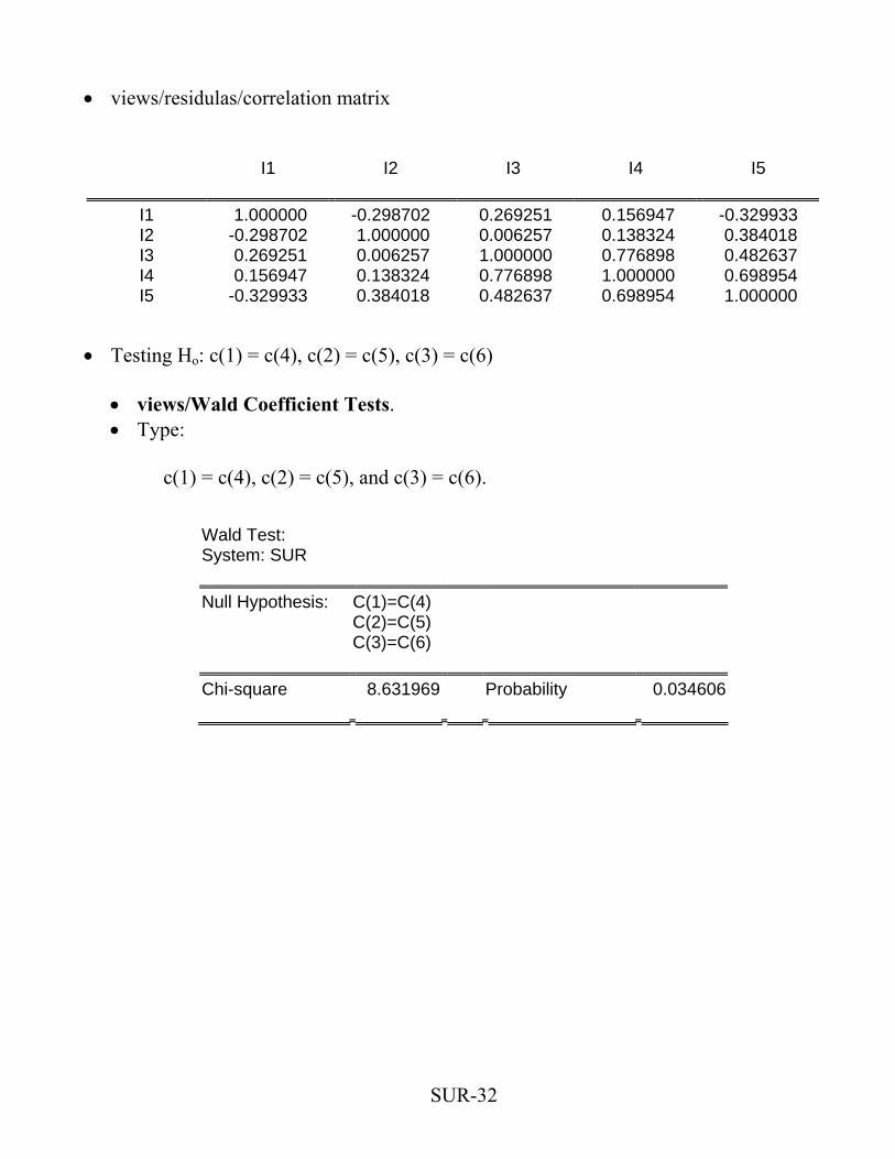
• views/residulas/correlation matrix
I1 I2 I3 I4 I5
I1 1.000000 -0.298702 0.269251 0.156947 -0.329933 I2 -0.298702 1.000000 0.006257 0.138324 0.384018 I3 0.269251 0.006257 1.000000 0.776898 0.482637 I4 0.156947 0.138324 0.776898 1.000000 0.698954 I5 -0.329933 0.384018 0.482637 0.698954 1.000000
• Testing Ho: c(1) = c(4), c(2) = c(5), c(3) = c(6) • views/Wald Coefficient Tests. • Type: c(1) = c(4), c(2) = c(5), and c(3) = c(6).
Wald Test: System: SUR
Null Hypothesis: C(1)=C(4)
C(2)=C(5) C(3)=C(6)
Chi-square 8.631969 Probability 0.034606
SUR-33
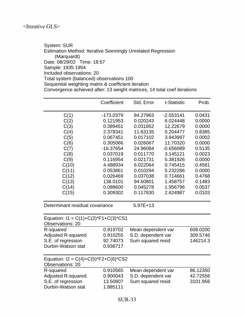
<Iterative GLS>
System: SUR Estimation Method: Iterative Seemingly Unrelated Regression (Marquardt) Date: 08/29/02 Time: 18:57 Sample: 1935 1954 Included observations: 20 Total system (balanced) observations 100 Sequential weighting matrix & coefficient iteration Convergence achieved after: 13 weight matrices, 14 total coef iterations
Coefficient Std. Error t-Statistic Prob.
C(1) -173.0379 84.27963 -2.053141 0.0431C(2) 0.121953 0.020243 6.024448 0.0000C(3) 0.389451 0.031852 12.22679 0.0000C(4) 2.378341 11.63135 0.204477 0.8385C(5) 0.067451 0.017102 3.943997 0.0002C(6) 0.305066 0.026067 11.70320 0.0000C(7) -16.37654 24.96084 -0.656089 0.5135C(8) 0.037019 0.011770 3.145121 0.0023C(9) 0.116954 0.021731 5.381926 0.0000C(10) 4.488934 6.022064 0.745415 0.4581C(11) 0.053861 0.010294 5.232286 0.0000C(12) 0.026469 0.037038 0.714661 0.4768C(13) 138.0101 94.60801 1.458757 0.1483C(14) 0.088600 0.045278 1.956796 0.0537C(15) 0.309302 0.117830 2.624987 0.0103
Determinant residual covariance 5.97E+13
Equation: I1 = C(1)+C(2)*F1+C(3)*CS1 Observations: 20 R-squared 0.919702 Mean dependent var 608.0200Adjusted R-squared 0.910255 S.D. dependent var 309.5746S.E. of regression 92.74073 Sum squared resid 146214.3Durbin-Watson stat 0.936717
Equation: I2 = C(4)+C(5)*F2+C(6)*CS2 Observations: 20 R-squared 0.910565 Mean dependent var 86.12350Adjusted R-squared 0.900043 S.D. dependent var 42.72556S.E. of regression 13.50807 Sum squared resid 3101.956Durbin-Watson stat 1.885111
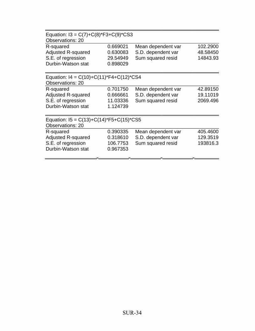
SUR-34
Equation: I3 = C(7)+C(8)*F3+C(9)*CS3 Observations: 20 R-squared 0.669021 Mean dependent var 102.2900Adjusted R-squared 0.630083 S.D. dependent var 48.58450S.E. of regression 29.54949 Sum squared resid 14843.93Durbin-Watson stat 0.898029
Equation: I4 = C(10)+C(11)*F4+C(12)*CS4 Observations: 20 R-squared 0.701750 Mean dependent var 42.89150Adjusted R-squared 0.666661 S.D. dependent var 19.11019S.E. of regression 11.03336 Sum squared resid 2069.496Durbin-Watson stat 1.124739
Equation: I5 = C(13)+C(14)*F5+C(15)*CS5 Observations: 20 R-squared 0.390335 Mean dependent var 405.4600Adjusted R-squared 0.318610 S.D. dependent var 129.3519S.E. of regression 106.7753 Sum squared resid 193816.3Durbin-Watson stat 0.967353
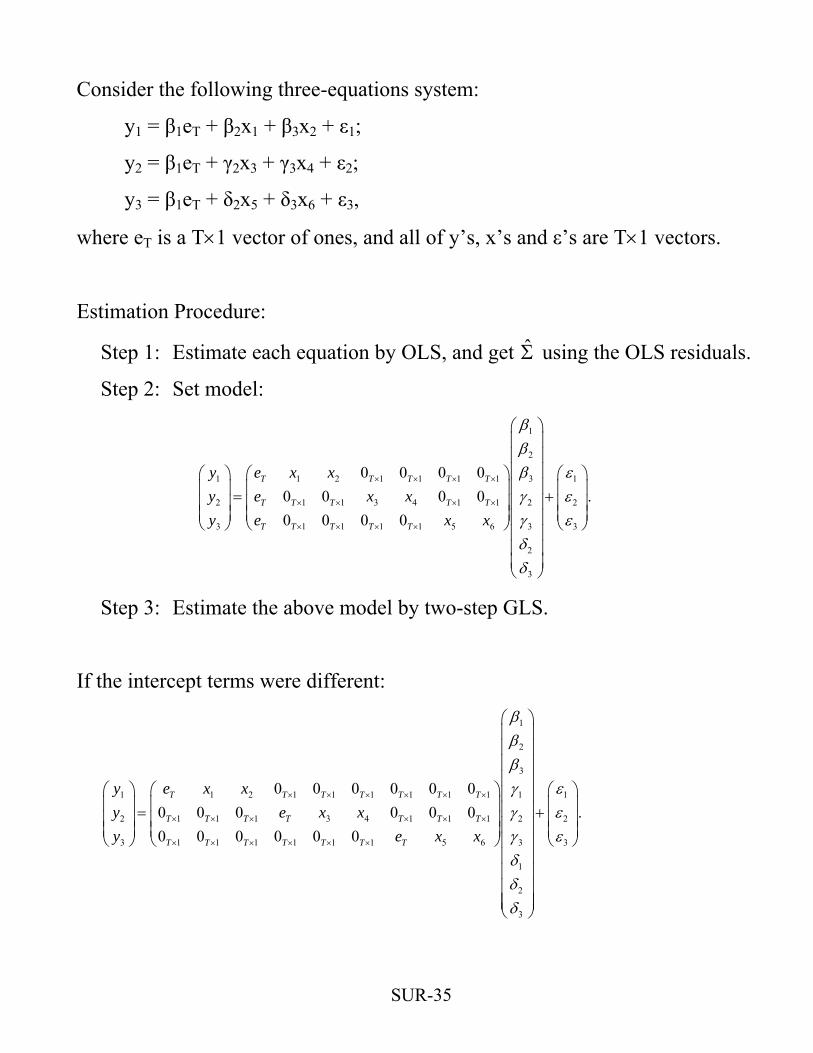
Consider the following three-equations system:
y1 = β1eT + β2x1 + β3x2 + ε1;
y2 = β1eT + γ2x3 + γ3x4 + ε2;
y3 = β1eT + δ2x5 + δ3x6 + ε3,
where eT is a T×1 vector of ones, and all of y’s, x’s and ε’s are T×1 vectors.
Estimation Procedure:
Step 1: Estimate each equation by OLS, and get Σ using the OLS residuals.
Step 2: Set model:
1
2
1 1 2 1 1 1 1 3
2 1 1 3 4 1 1 2
3 1 1 1 1 5 6 3 3
2
3
0 0 0 00 0 0 00 0 0 0
T T T T T
T T T T T
T T T T T
y e x xy e x xy e x x
ββ
1
2 .β εγ εγ εδδ
× × × ×
× × × ×
× × × ×
⎛ ⎞⎜ ⎟⎜ ⎟⎜ ⎟⎛ ⎞ ⎛ ⎞ ⎛ ⎞⎜ ⎟⎜ ⎟ ⎜ ⎟ ⎜ ⎟= +⎜ ⎟⎜ ⎟ ⎜ ⎟ ⎜ ⎟
⎜ ⎟ ⎜ ⎟ ⎜ ⎟⎜ ⎟⎝ ⎠ ⎝ ⎠ ⎝ ⎠⎜ ⎟⎜ ⎟⎜ ⎟⎝ ⎠
Step 3: Estimate the above model by two-step GLS.
If the intercept terms were different:
1
2
3
1 1 2 1 1 1 1 1 1 1 1
2 1 1 1 3 4 1 1 1 2 2
3 1 1 1 1 1 1 5 6 3 3
1
2
3
0 0 0 0 0 00 0 0 0 0 00 0 0 0 0 0
T T T T T T T
T T T T T T T
T T T T T T T
y e x xy e x xy e x
βββ
.x
γ εγ εγ εδδδ
× × × × × ×
× × × × × ×
× × × × × ×
⎛ ⎞⎜ ⎟⎜ ⎟⎜ ⎟⎜ ⎟
⎛ ⎞ ⎛ ⎞ ⎛ ⎞⎜ ⎟⎜ ⎟ ⎜ ⎟ ⎜ ⎟⎜ ⎟= +⎜ ⎟ ⎜ ⎟ ⎜ ⎟⎜ ⎟⎜ ⎟ ⎜ ⎟ ⎜ ⎟⎝ ⎠ ⎝ ⎠ ⎝ ⎠⎜ ⎟
⎜ ⎟⎜ ⎟⎜ ⎟⎜ ⎟⎜ ⎟⎝ ⎠
SUR-35
![3. SEEMINGLY UNRELATED REGRESSIONS (SUR) - …miniahn/ecn726/cn_sur.pdf · SUR-1 3. SEEMINGLY UNRELATED REGRESSIONS (SUR) [1] Examples • Demand for some commodities: yNike,t = xNike,t′βNike](https://static.fdocument.org/doc/165x107/5b2a264d7f8b9ad8298b90a2/3-seemingly-unrelated-regressions-sur-miniahnecn726cnsurpdf-sur-1-3.jpg)


![SELF-SHRINKERS TO THE MEAN CURVATURE FLOW …js/isoparametric.shrinker.final.pdf · This is a seemingly ill-posed problem since by the uniqueness theorem of Lu Wang [21], we cannot](https://static.fdocument.org/doc/165x107/60fb01b2d1ad03084b7f1a93/self-shrinkers-to-the-mean-curvature-flow-js-this-is-a-seemingly-ill-posed-problem.jpg)


![Effects of Seeding on Lysozyme Amyloid Fibrillation in the ... · Alzheimer’s disease, type 2 diabetes, and several systemic amyloidoses [1-3]. These proteins, despite their unrelated](https://static.fdocument.org/doc/165x107/5f66a2f7828269373b7d097b/effects-of-seeding-on-lysozyme-amyloid-fibrillation-in-the-alzheimeras-disease.jpg)