3 - Choosing the Right Method - Benzene Dimerekwan/computational pdfs/3 - Choosing...Choosing The...
15
Chem 106: Computational Handout 3 Choosing The Right Method: Benzene Dimer Objectives: single point energy calculations, simple scripting, dispersion, counterpoise correction In This Exercise: we will consider the T-shaped dimer of benzene, a prototype for π-stacking. This complex is bound by approximately 2.7 kcal/mol. We will calculate the binding energy as a function of the distance between the monomers and determine what the appropriate computational method in this system is. Reference: This exercise uses some data published by the Sherrill group (JPCA 2004, 108, 10200). David Sherrill (Georgia) is a leader in studying non-covalent interactions with coupled cluster methods and has published many interesting papers in this area. Background: One can consider several possible conformations for benzene dimer: Sherill and others have shown that the T-shaped and parallel-displaced geometries are roughly isoenergetic local minima, while the sandwich geometry is a transition state that is higher in energy by about 0.7 kcal/mol. Here, we will only consider the T-shaped geometry. In benzene monomer, the charge distribution is controlled by electronegativity. Carbon is more electronegative than hydrogen, so benzene’s charge distribution is roughly quadrupolar: a negative charged surface over the ring and a positively charged periphery. In the T-shaped dimer, there is a favorable interaction between the face of one ring and the edge of another. We must also consider two other effects: London dispersion (attractive, caused by instantaneously correlated fluctuations in electron density in both monomers) and van der Waals forces (repulsive, and can be thought of the cost of the extra curvature in the wave function needed to keep the orbitals orthogonal). Although electrostatic and van der Waals forces are treated accurately by most computational methods, London dispersion forces are problematic because they involve electron correlation. Until recently, this was considered a major failure of density functional theory (DFT). H H H H
-
Upload
hoangkhanh -
Category
Documents
-
view
223 -
download
0
Transcript of 3 - Choosing the Right Method - Benzene Dimerekwan/computational pdfs/3 - Choosing...Choosing The...
Chem 106: Computational Handout 3 Choosing The Right Method: Benzene Dimer
Objectives: single point energy calculations, simple scripting, dispersion, counterpoise correction
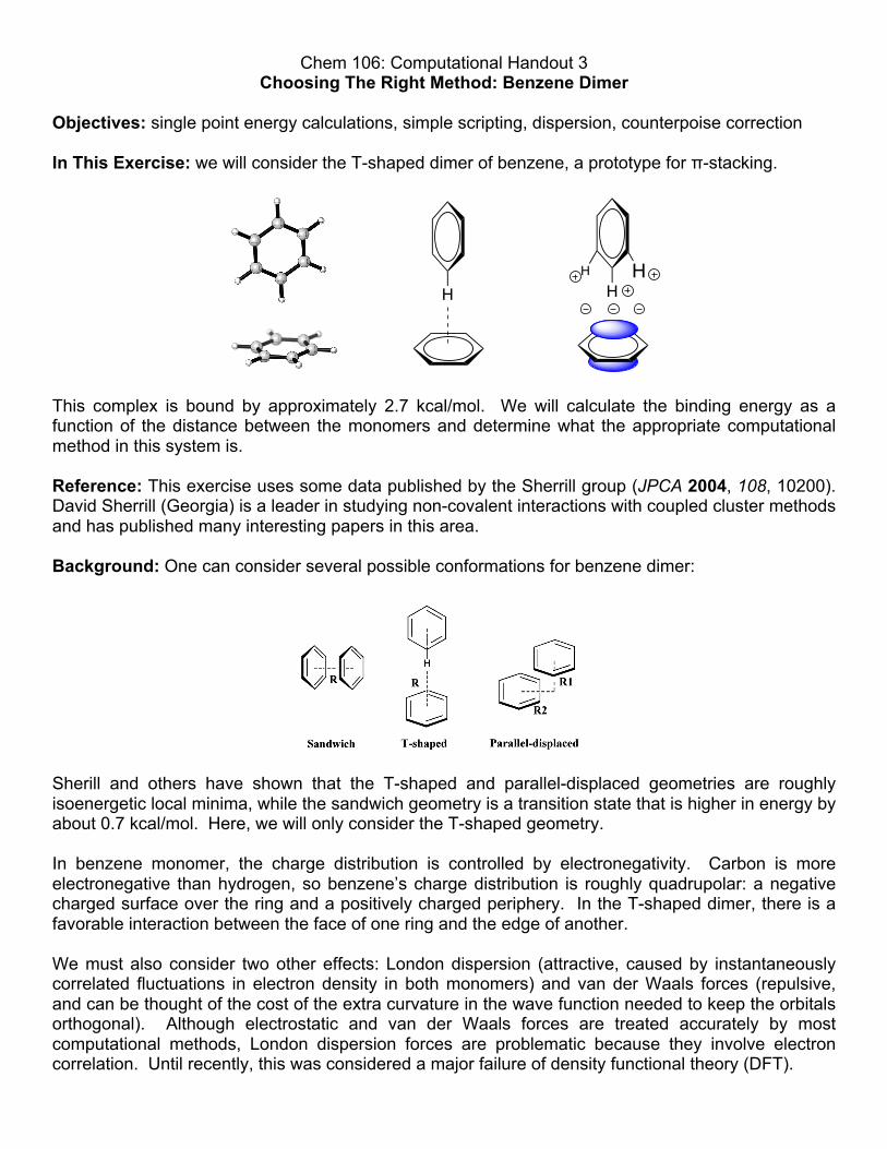
In This Exercise: we will consider the T-shaped dimer of benzene, a prototype for π-stacking.
This complex is bound by approximately 2.7 kcal/mol. We will calculate the binding energy as a function of the distance between the monomers and determine what the appropriate computational method in this system is. Reference: This exercise uses some data published by the Sherrill group (JPCA 2004, 108, 10200). David Sherrill (Georgia) is a leader in studying non-covalent interactions with coupled cluster methods and has published many interesting papers in this area. Background: One can consider several possible conformations for benzene dimer:
Sherill and others have shown that the T-shaped and parallel-displaced geometries are roughly isoenergetic local minima, while the sandwich geometry is a transition state that is higher in energy by about 0.7 kcal/mol. Here, we will only consider the T-shaped geometry. In benzene monomer, the charge distribution is controlled by electronegativity. Carbon is more electronegative than hydrogen, so benzene’s charge distribution is roughly quadrupolar: a negative charged surface over the ring and a positively charged periphery. In the T-shaped dimer, there is a favorable interaction between the face of one ring and the edge of another. We must also consider two other effects: London dispersion (attractive, caused by instantaneously correlated fluctuations in electron density in both monomers) and van der Waals forces (repulsive, and can be thought of the cost of the extra curvature in the wave function needed to keep the orbitals orthogonal). Although electrostatic and van der Waals forces are treated accurately by most computational methods, London dispersion forces are problematic because they involve electron correlation. Until recently, this was considered a major failure of density functional theory (DFT).
H HH H
Setup: Login to Odyssey. Locally, start GaussView. There are many jobs to run in this exercise. If you run into problems, you can work with the output files I got. These files are stored in chem106_calculations/benzene/out. The input files are located in the neighboring gjf folder. Further Exploration: These jobs were generated using templates and scripts in the prep folder. These can be easily modified to explore related systems or other levels of theory, but the details of this are too complicated for this exercise. If you want to pursue this, I would be happy to assist you. Examine Input Files 1. Update your local chem106_calculations git repository: cd ~/chem106_calculations git pull
2. Make a copy of the benzene folder and work with it somewhere else: cp -r ~/chem106_calculations/benzene ~/benzene cd benzene/gjf
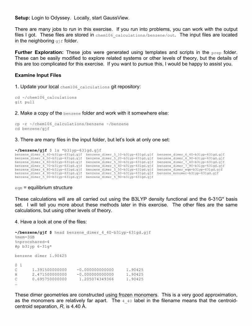
3. There are many files in the input folder, but let’s look at only one set: ~/benzene/gjf $ ls *b3lyp-631gd.gjf benzene_dimer_4_40-b3lyp-631gd.gjf benzene_dimer_5_10-b3lyp-631gd.gjf benzene_dimer_6_40-b3lyp-631gd.gjf benzene_dimer_4_50-b3lyp-631gd.gjf benzene_dimer_5_20-b3lyp-631gd.gjf benzene_dimer_6_90-b3lyp-631gd.gjf benzene_dimer_4_60-b3lyp-631gd.gjf benzene_dimer_5_30-b3lyp-631gd.gjf benzene_dimer_7_40-b3lyp-631gd.gjf benzene_dimer_4_70-b3lyp-631gd.gjf benzene_dimer_5_40-b3lyp-631gd.gjf benzene_dimer_7_90-b3lyp-631gd.gjf benzene_dimer_4_80-b3lyp-631gd.gjf benzene_dimer_5_50-b3lyp-631gd.gjf benzene_dimer_eqm-b3lyp-631gd.gjf benzene_dimer_4_90-b3lyp-631gd.gjf benzene_dimer_5_60-b3lyp-631gd.gjf benzene_monomer-b3lyp-631gd.gjf benzene_dimer_5_00-b3lyp-631gd.gjf benzene_dimer_5_90-b3lyp-631gd.gjf
eqm = equilibrium structure These calculations will are all carried out using the B3LYP density functional and the 6-31G* basis set. I will tell you more about these methods later in this exercise. The other files are the same calculations, but using other levels of theory. 4. Have a look at one of the files: ~/benzene/gjf $ head benzene_dimer_4_40-b3lyp-631gd.gjf %mem=3GB %nprocshared=4 #p b3lyp 6-31g* benzene dimer 1.90425 0 1 C 1.391500000000 -0.000000000000 1.90425 H 2.471500000000 -0.000000000000 1.90425 C 0.695750000000 1.205074349366 1.90425 …
These dimer geometries are constructed using frozen monomers. This is a very good approximation, as the monomers are relatively far apart. The 4_40 label in the filename means that the centroid-centroid separation, R, is 4.40 Å.
%nprocshared=4 means that we are requesting that 4 processors work together simultaneously to complete this particular calculation. The lack of the opt keyword means that this is a “single point energy” calculation. In English: calculate the energy of this geometry, but don’t optimize it. All the calculations use the same geometries so that their relative energies can be compared. Run Jobs 1. Update your chem106_calculations git repository on Odyssey with git pull. 2. All the files follow a common naming pattern: ~/chem106_calculations/benzene/gjf $ ls -l *4_40*.gjf | awk '{print $NF}' benzene_dimer_4_40-b3lyp-631gd-cp.gjf benzene_dimer_4_40-b3lyp-631gd.gjf benzene_dimer_4_40-b3lyp_d3bj-631gd-cp.gjf benzene_dimer_4_40-b3lyp_d3bj-631gd.gjf benzene_dimer_4_40-b3lyp_d3bj-dz.gjf benzene_dimer_4_40-b3lyp_d3bj-juldz.gjf benzene_dimer_4_40-b3lyp_d3bj-juntz.gjf benzene_dimer_4_40-b3lyp_d3bj-mayqz.gjf benzene_dimer_4_40-b3lyp_d3bj-qz.gjf benzene_dimer_4_40-b3lyp_d3bj-tz.gjf benzene_dimer_4_40-hf-631gd-cp.gjf benzene_dimer_4_40-hf-631gd.gjf benzene_dimer_4_40-m062x-631gd-cp.gjf benzene_dimer_4_40-m062x-631gd.gjf benzene_dimer_4_40-m062x-mayqz.gjf benzene_dimer_4_40-mp2-631gd-cp.gjf benzene_dimer_4_40-mp2-631gd.gjf benzene_dimer_4_40-pbe0_d3bj-631gd.gjf benzene_dimer_4_40-pbe0_d3bj-mayqz.gjf
ls -l requests a list of files with more information (take away the pipe and the stuff after it to see for yourself). We are only looking at filenames containing 4_40. We are piping the result to awk, which is printing only the last field ($NF, where NF is a special awk variable that is the number of fields). If we consider the filenames as fields separated by dashes (but not underscores), then the second field is the name of the method. Here is a legend: DFT methods: B3LYP, M06-2X, PBE0 ab initio methods: HF (Hartree–Fock), MP2 (Moller–Plesset perturbation theory, second order) Files ending in -cp mean counterpoise correction files (used later in this exercise). 3. Run the jobs ending with b3lyp-631gd.out. Examine Output Files 1. In GaussView, open up the *b3lyp-631gd.out files. Extract the electronic energies from Results…Summary. Alternatively, use grep (look for SCF Done). 2. Compute the relative energies in Excel. Reminder: 1 hartree = 627.509469 kcal/mol.
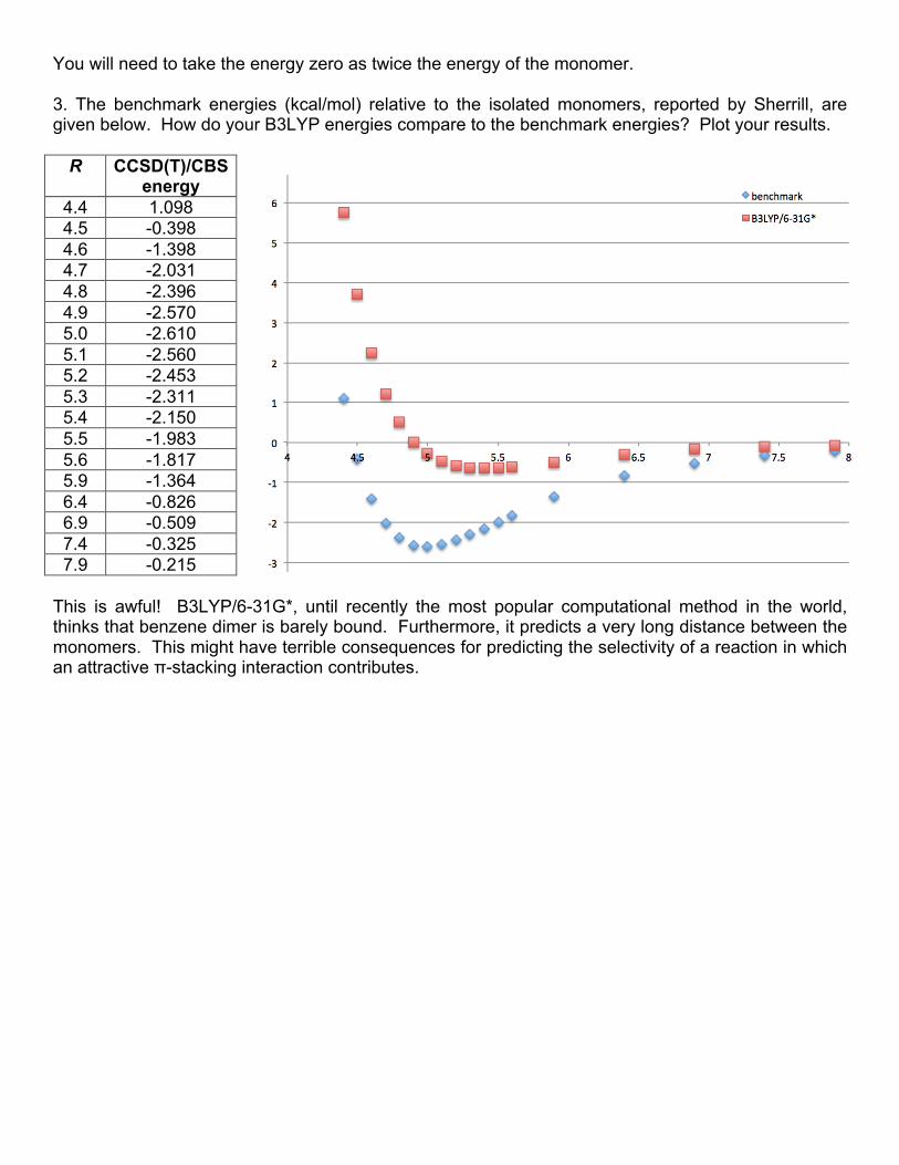
You will need to take the energy zero as twice the energy of the monomer. 3. The benchmark energies (kcal/mol) relative to the isolated monomers, reported by Sherrill, are given below. How do your B3LYP energies compare to the benchmark energies? Plot your results.
R CCSD(T)/CBS energy
4.4 1.098 4.5 -0.398 4.6 -1.398 4.7 -2.031 4.8 -2.396 4.9 -2.570 5.0 -2.610 5.1 -2.560 5.2 -2.453 5.3 -2.311 5.4 -2.150 5.5 -1.983 5.6 -1.817 5.9 -1.364 6.4 -0.826 6.9 -0.509 7.4 -0.325 7.9 -0.215
This is awful! B3LYP/6-31G*, until recently the most popular computational method in the world, thinks that benzene dimer is barely bound. Furthermore, it predicts a very long distance between the monomers. This might have terrible consequences for predicting the selectivity of a reaction in which an attractive π-stacking interaction contributes.
Counterpoise Correction See http://vergil.chemistry.gatech.edu/notes/cp.pdf for an excellent discussion. 6-31G* was popularized by John Pople (Nobel Prize, 1998) in the early 1970s and is widely used today. However, it is not appropriate for all purposes because of its small size. Basis sets are collections of mathematical functions (specifically Gaussian functions, hence the “G”) that are used to describe wavefunctions. Because wavefunctions have a cusp at the nucleus, many Gaussians must be added together to describe the true wavefunction properly. The larger the basis set, the more mathematical flexibility is available to describe the cusp. The difference between the energy obtained with a finite basis set and the energy that would be obtained with an infinite basis set is called basis set incompleteness error (BSIE). Basis set incompleteness leads to a peculiar problem called basis set superposition error (BSSE). The idea stems from the variational principle,1 which states that when more orbitals are available to describe the wavefunction, the energy goes down and becomes closer to the true energy. The intuition for the principle is as follows. The energy of the correct wavefunction is the exact ground state energy. Any approximate wavefunction can be described as a linear combination of the true ground state wavefunction and excited states. Similarly, the energy of an approximate wavefunction is a linear combination of the energies of the ground state energy (the lowest energy) and the excited state energies (higher). Therefore, any approximate wavefunction will have an energy that is larger than the true ground state wavefunction. When more orbitals are added, the approximation becomes better and better, and the energy drops. BSSE occurs when calculating the interaction energy of two monomers. It arises from the increase in effective basis set size as the interaction distance decreases. Monomers are able to “use” the basis functions from one another at short distances, but not at long distances. This inconsistency leads to an artificial over-binding of non-covalent complexes. The Boys–Bernardi counterpoise correction seeks to remove BSSE by taking the true interaction energy as:
ΔEint = EAB AB( )−EA A( )−EB B( )− ΔECPΔECP = EAB A( )−EA A( )⎡⎣ ⎤⎦+ EAB B( )−EB B( )⎡⎣ ⎤⎦
The subscripts denote the basis set: AB means placing basis functions at the locations of the atoms in the complex, regardless of whether there are atoms there or not. For example, EAB(A) is the energy of monomer A, but with basis functions at the locations of both monomers. In this case, the basis functions at the location of monomer B are called “ghost orbitals.” Effectively, the counterpoise correction takes into account the extra lowering in energy induced by the presence of the other monomer. The correction is not perfect. It can overcorrect because the orbitals in monomer A are not really completely available to monomer B in the complex due to Pauli repulsion. It also does not remove BSIE. It should be noted that intramolecular BSSE also exists and cannot be ignored. Unfortunately, it is harder to correct for because there is no obvious way to divide up the fragments. Also, both inter- and intramolecular BSSE are quite expensive to correct for. Grimme and co-workers have recently devised a “geometrical counterpoise” correction that uses a very fast atom-based strategy and
1Notallcomputationalmethodsobeythevariationalprinciple,butthisisausefulwaytothinkabouttheproblem.
several empirical parameters that seeks to solve some of these problems. Please see http://www.thch.uni-bonn.de/tc/downloads/gcp/ for more details. In the following steps, we will see what the influence of intermolecular BSSE is on the benzene dimer. 1. The B3LYP/6-31G* we calculated above shows a shallow minimum. Is this the result of underestimating the dispersion interaction, or merely an artifact of BSSE? Let’s examine the energies with the counterpoise correction. ~/benzene/gjf $ more benzene_dimer_5_40-b3lyp-631gd-cp.gjf %mem=3GB %nprocshared=4 #p counterpoise=2 b3lyp 6-31g* benzene dimer 2.90425 0 1 C(Fragment=1) 1.391500000000 -0.000000000000 2.90425 H(Fragment=1) 2.471500000000 -0.000000000000 2.90425 … C(Fragment=2) 0.000000000000 0.000000000000 -1.104250000000 C(Fragment=2) -0.000000000000 -1.205074349366 -1.800000000000 …
The input file has a new keyword counterpoise=2, which calls for a two-fragment counterpoise correction. Each atom is marked with a label to tell Gaussian whether it is in fragment 1 or 2. 2. Run the jobs ending in b3lyp-631gd-cp.gjf. 3. Let’s extract the energies again. There is no way to do this from GaussView, so we have to do it from the command-line. The counterpoise results are written out on lines like this: ~/benzene/out $ grep -A4 "Counterpoise corrected energy" benzene_dimer_5_40-b3lyp-631gd-cp.out Counterpoise corrected energy = -464.496737221051 BSSE energy = 0.000883787183 sum of monomers = -464.496624297245 complexation energy = -0.63 kcal/mole (raw) complexation energy = -0.07 kcal/mole (corrected)
grep is a tool for searching files for text. Here, we are looking for the phrase Counterpoise corrected energy in the specified file. The -A flag means that we are asking grep to show us 4 lines after each hit. 4. It will be tedious to do this one file a time, so let’s speed this up: ~/chem106_calculations/benzene/out $ grep \(corrected *b3lyp-631gd-cp.out benzene_dimer_4_40-b3lyp-631gd-cp.out: complexation energy = 7.29 kcal/mole (corrected) benzene_dimer_4_50-b3lyp-631gd-cp.out: complexation energy = 5.12 kcal/mole (corrected) benzene_dimer_4_60-b3lyp-631gd-cp.out: complexation energy = 3.52 kcal/mole (corrected) … benzene_dimer_eqm-b3lyp-631gd-cp.out: complexation energy = 0.59 kcal/mole (corrected)
This time, we only want one line per file, so we didn’t include the -A flag. We need a backslash (\) before the ( because parentheses have special meaning to grep, and we just mean a literal (. In general, placing a backslash before a character to specify the literal character is called “escaping a character.”
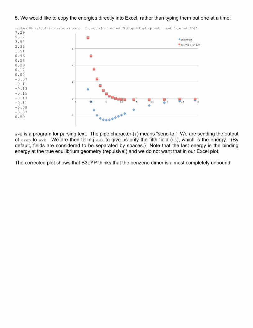
5. We would like to copy the energies directly into Excel, rather than typing them out one at a time: ~/chem106_calculations/benzene/out $ grep \(corrected *b3lyp-631gd-cp.out | awk '{print $5}' 7.29 5.12 3.52 2.36 1.54 0.96 0.56 0.29 0.12 0.00 -0.07 -0.11 -0.13 -0.15 -0.13 -0.11 -0.09 -0.07 0.59
awk is a program for parsing text. The pipe character (|) means “send to.” We are sending the output of grep to awk. We are then telling awk to give us only the fifth field ($5), which is the energy. (By default, fields are considered to be separated by spaces.) Note that the last energy is the binding energy at the true equilibrium geometry (repulsive!) and we do not want that in our Excel plot. The corrected plot shows that B3LYP thinks that the benzene dimer is almost completely unbound!
Dispersion Corrections The problem with B3LYP is that it has no ability to treat dispersion. B3LYP only uses local quantities such as the electron density and its derivatives at a particular position to calculate the energy. Because dispersion is fundamentally a non-local phenomenon of electron correlation, B3LYP is unable to correct for it. Fortunately, there are now a number of approaches to dealing with dispersion that are quite practical. See Grimme Chem. Rev. 2016, 116, 5105 for a comprehensive discussion. We will take the most popular approach, which is to add a Lennard–Jones-type correction to the energy. In particular, we will use the “-D3(BJ)” recipe of Grimme. In English, this is a dispersion correction that involves both two- and three-body dispersion, and it uses Becke–Johnson damping to prevent the correction from blowing up at short distances. 1. Let’s examine B3LYP-D3BJ/6-31G* without counterpoise correction first. Run the files ending in b3lyp_d3bj-631gd.out. 2. To speed things up, I have written a short awk script to calculate the relative energies: ~/chem106_calculations/benzene/out $ awk -f extract.awk *-b3lyp_d3bj-631gd.out benzene_dimer_4_40-b3lyp_d3bj-631gd.out -0.23 benzene_dimer_4_50-b3lyp_d3bj-631gd.out -1.77 …
This reports the energies in kcal/mol relative to the monomer. To speed up the pasting process, pipe the results to awk. The -f syntax here tells awk to run commands from a script, extract.awk, instead of the command line. Any arguments after the name of the awk script to run are treated as files to be read by awk. 3. (Optional Reading) How does the awk script work? awk takes a series of files and processes them one line at a time. Each section of an awk script has a pattern and an action. A pattern is some condition or piece of text, which if found, will trigger some code (the action). Here is the script, broken down into sections and explained: FNR == 1 { file_count++ filename[file_count] = FILENAME }
When reads the first file, it increments the special awk variables NR and FNR once per line. When it gets to the second file, NR keeps going up, but FNR starts again at 1. So, the pattern here of FNR == 1 means “if we are on the first line of a file.” FILENAME is also a special awk variable that stores the name of the current file. Here, the action is to store the filenames into an array called filename. Thus, filename[1] will contain the name of the first file, filename[2] the name of the second file, and so forth.
/SCF Done/ { if ( match(FILENAME,"monomer") > 0 ) zero=2.0*$5 energy[file_count] = $5 }
The pattern here is to look for the text SCF Done. In awk, text patterns are enclosed inside forward slashes. The action is to store the energy, the fifth field ($5), in an array called energy. In the special case that the filename contains monomer, we keep track of the “zero” of energy. END { for (i=1; i <= file_count; i++) { if ( match(filename[i], "monomer") > 0 ) continue printf "%50-s %5.2f\n", filename[i], (energy[i]-zero)*627.509469 } }
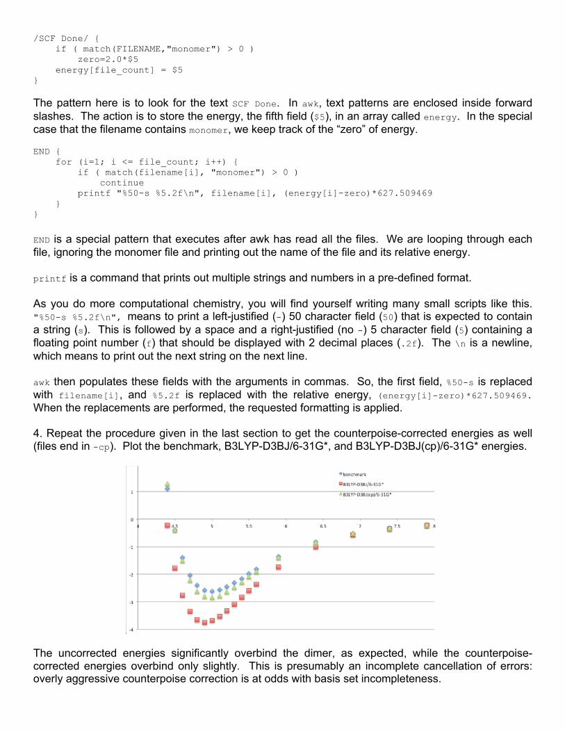
END is a special pattern that executes after awk has read all the files. We are looping through each file, ignoring the monomer file and printing out the name of the file and its relative energy. printf is a command that prints out multiple strings and numbers in a pre-defined format. As you do more computational chemistry, you will find yourself writing many small scripts like this. "%50-s %5.2f\n", means to print a left-justified (-) 50 character field (50) that is expected to contain a string (s). This is followed by a space and a right-justified (no -) 5 character field (5) containing a floating point number (f) that should be displayed with 2 decimal places (.2f). The \n is a newline, which means to print out the next string on the next line. awk then populates these fields with the arguments in commas. So, the first field, %50-s is replaced with filename[i], and %5.2f is replaced with the relative energy, (energy[i]-zero)*627.509469. When the replacements are performed, the requested formatting is applied. 4. Repeat the procedure given in the last section to get the counterpoise-corrected energies as well (files end in -cp). Plot the benchmark, B3LYP-D3BJ/6-31G*, and B3LYP-D3BJ(cp)/6-31G* energies.
The uncorrected energies significantly overbind the dimer, as expected, while the counterpoise-corrected energies overbind only slightly. This is presumably an incomplete cancellation of errors: overly aggressive counterpoise correction is at odds with basis set incompleteness.
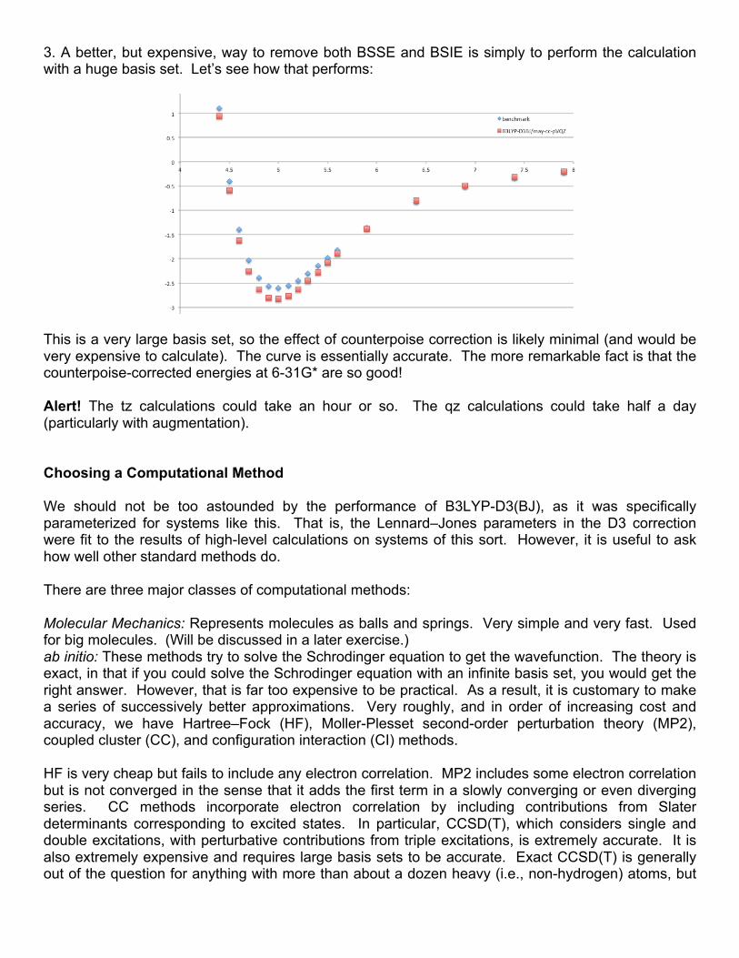
3. A better, but expensive, way to remove both BSSE and BSIE is simply to perform the calculation with a huge basis set. Let’s see how that performs:
This is a very large basis set, so the effect of counterpoise correction is likely minimal (and would be very expensive to calculate). The curve is essentially accurate. The more remarkable fact is that the counterpoise-corrected energies at 6-31G* are so good! Alert! The tz calculations could take an hour or so. The qz calculations could take half a day (particularly with augmentation). Choosing a Computational Method We should not be too astounded by the performance of B3LYP-D3(BJ), as it was specifically parameterized for systems like this. That is, the Lennard–Jones parameters in the D3 correction were fit to the results of high-level calculations on systems of this sort. However, it is useful to ask how well other standard methods do. There are three major classes of computational methods: Molecular Mechanics: Represents molecules as balls and springs. Very simple and very fast. Used for big molecules. (Will be discussed in a later exercise.) ab initio: These methods try to solve the Schrodinger equation to get the wavefunction. The theory is exact, in that if you could solve the Schrodinger equation with an infinite basis set, you would get the right answer. However, that is far too expensive to be practical. As a result, it is customary to make a series of successively better approximations. Very roughly, and in order of increasing cost and accuracy, we have Hartree–Fock (HF), Moller-Plesset second-order perturbation theory (MP2), coupled cluster (CC), and configuration interaction (CI) methods. HF is very cheap but fails to include any electron correlation. MP2 includes some electron correlation but is not converged in the sense that it adds the first term in a slowly converging or even diverging series. CC methods incorporate electron correlation by including contributions from Slater determinants corresponding to excited states. In particular, CCSD(T), which considers single and double excitations, with perturbative contributions from triple excitations, is extremely accurate. It is also extremely expensive and requires large basis sets to be accurate. Exact CCSD(T) is generally out of the question for anything with more than about a dozen heavy (i.e., non-hydrogen) atoms, but
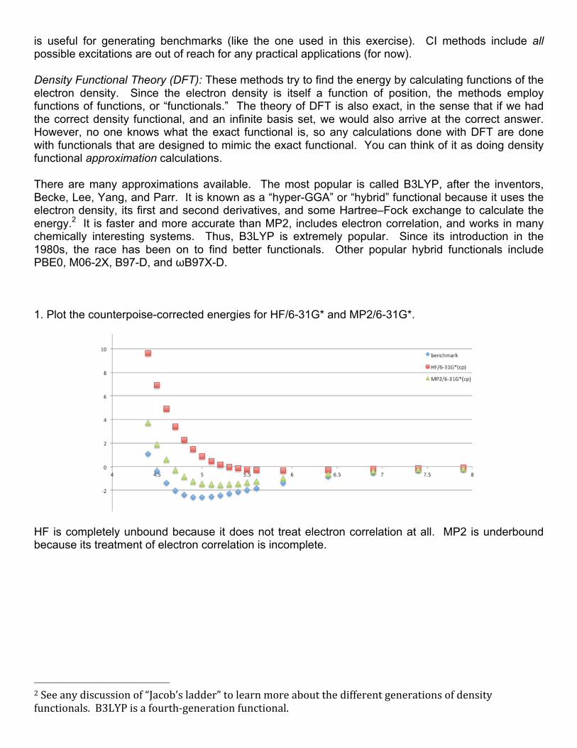
is useful for generating benchmarks (like the one used in this exercise). CI methods include all possible excitations are out of reach for any practical applications (for now). Density Functional Theory (DFT): These methods try to find the energy by calculating functions of the electron density. Since the electron density is itself a function of position, the methods employ functions of functions, or “functionals.” The theory of DFT is also exact, in the sense that if we had the correct density functional, and an infinite basis set, we would also arrive at the correct answer. However, no one knows what the exact functional is, so any calculations done with DFT are done with functionals that are designed to mimic the exact functional. You can think of it as doing density functional approximation calculations. There are many approximations available. The most popular is called B3LYP, after the inventors, Becke, Lee, Yang, and Parr. It is known as a “hyper-GGA” or “hybrid” functional because it uses the electron density, its first and second derivatives, and some Hartree–Fock exchange to calculate the energy.2 It is faster and more accurate than MP2, includes electron correlation, and works in many chemically interesting systems. Thus, B3LYP is extremely popular. Since its introduction in the 1980s, the race has been on to find better functionals. Other popular hybrid functionals include PBE0, M06-2X, B97-D, and ωB97X-D. 1. Plot the counterpoise-corrected energies for HF/6-31G* and MP2/6-31G*.
HF is completely unbound because it does not treat electron correlation at all. MP2 is underbound because its treatment of electron correlation is incomplete.
2Seeanydiscussionof“Jacob’sladder”tolearnmoreaboutthedifferentgenerationsofdensityfunctionals.B3LYPisafourth-generationfunctional.
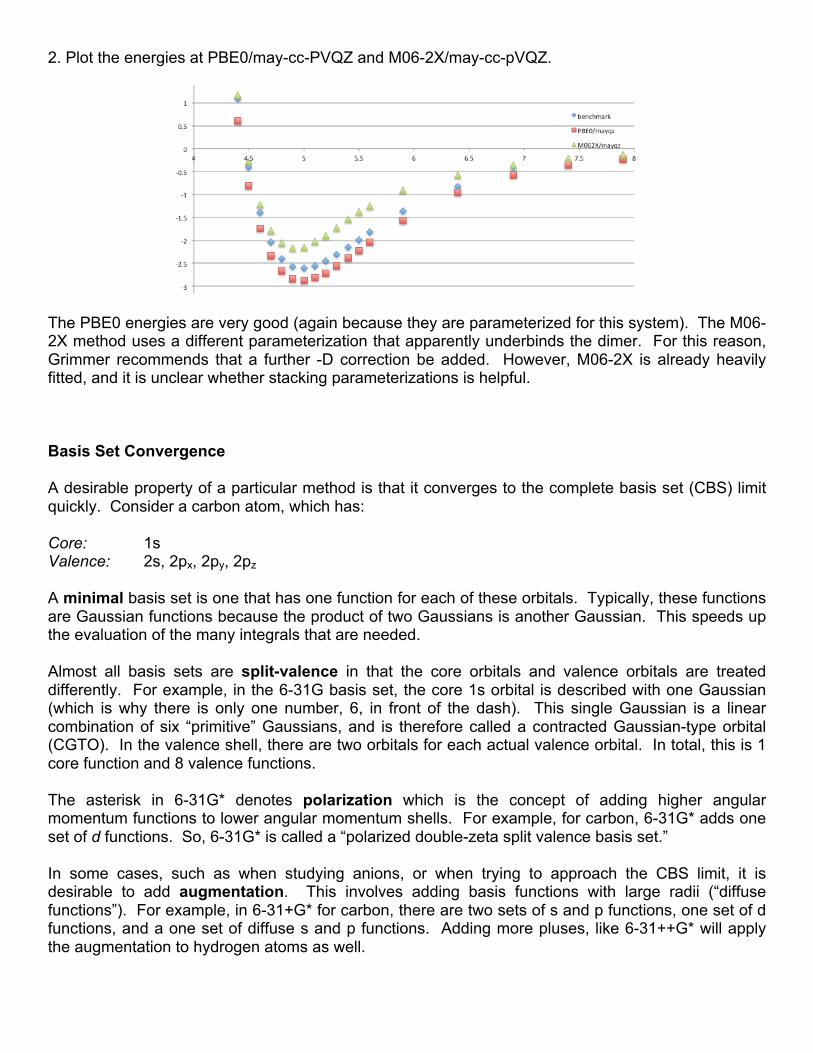
2. Plot the energies at PBE0/may-cc-PVQZ and M06-2X/may-cc-pVQZ.
The PBE0 energies are very good (again because they are parameterized for this system). The M06-2X method uses a different parameterization that apparently underbinds the dimer. For this reason, Grimmer recommends that a further -D correction be added. However, M06-2X is already heavily fitted, and it is unclear whether stacking parameterizations is helpful. Basis Set Convergence A desirable property of a particular method is that it converges to the complete basis set (CBS) limit quickly. Consider a carbon atom, which has: Core: 1s Valence: 2s, 2px, 2py, 2pz A minimal basis set is one that has one function for each of these orbitals. Typically, these functions are Gaussian functions because the product of two Gaussians is another Gaussian. This speeds up the evaluation of the many integrals that are needed. Almost all basis sets are split-valence in that the core orbitals and valence orbitals are treated differently. For example, in the 6-31G basis set, the core 1s orbital is described with one Gaussian (which is why there is only one number, 6, in front of the dash). This single Gaussian is a linear combination of six “primitive” Gaussians, and is therefore called a contracted Gaussian-type orbital (CGTO). In the valence shell, there are two orbitals for each actual valence orbital. In total, this is 1 core function and 8 valence functions. The asterisk in 6-31G* denotes polarization which is the concept of adding higher angular momentum functions to lower angular momentum shells. For example, for carbon, 6-31G* adds one set of d functions. So, 6-31G* is called a “polarized double-zeta split valence basis set.” In some cases, such as when studying anions, or when trying to approach the CBS limit, it is desirable to add augmentation. This involves adding basis functions with large radii (“diffuse functions”). For example, in 6-31+G* for carbon, there are two sets of s and p functions, one set of d functions, and a one set of diffuse s and p functions. Adding more pluses, like 6-31++G* will apply the augmentation to hydrogen atoms as well.
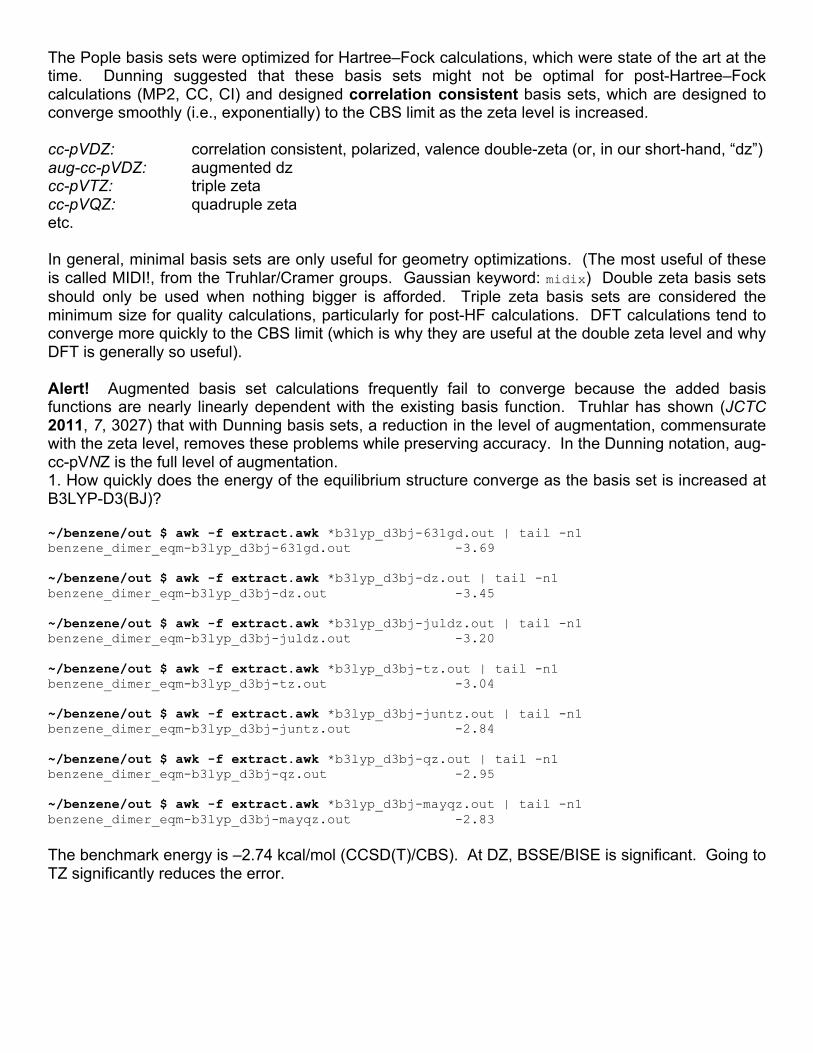
The Pople basis sets were optimized for Hartree–Fock calculations, which were state of the art at the time. Dunning suggested that these basis sets might not be optimal for post-Hartree–Fock calculations (MP2, CC, CI) and designed correlation consistent basis sets, which are designed to converge smoothly (i.e., exponentially) to the CBS limit as the zeta level is increased. cc-pVDZ: correlation consistent, polarized, valence double-zeta (or, in our short-hand, “dz”) aug-cc-pVDZ: augmented dz cc-pVTZ: triple zeta cc-pVQZ: quadruple zeta etc. In general, minimal basis sets are only useful for geometry optimizations. (The most useful of these is called MIDI!, from the Truhlar/Cramer groups. Gaussian keyword: midix) Double zeta basis sets should only be used when nothing bigger is afforded. Triple zeta basis sets are considered the minimum size for quality calculations, particularly for post-HF calculations. DFT calculations tend to converge more quickly to the CBS limit (which is why they are useful at the double zeta level and why DFT is generally so useful). Alert! Augmented basis set calculations frequently fail to converge because the added basis functions are nearly linearly dependent with the existing basis function. Truhlar has shown (JCTC 2011, 7, 3027) that with Dunning basis sets, a reduction in the level of augmentation, commensurate with the zeta level, removes these problems while preserving accuracy. In the Dunning notation, aug-cc-pVNZ is the full level of augmentation. 1. How quickly does the energy of the equilibrium structure converge as the basis set is increased at B3LYP-D3(BJ)? ~/benzene/out $ awk -f extract.awk *b3lyp_d3bj-631gd.out | tail -n1 benzene_dimer_eqm-b3lyp_d3bj-631gd.out -3.69 ~/benzene/out $ awk -f extract.awk *b3lyp_d3bj-dz.out | tail -n1 benzene_dimer_eqm-b3lyp_d3bj-dz.out -3.45 ~/benzene/out $ awk -f extract.awk *b3lyp_d3bj-juldz.out | tail -n1 benzene_dimer_eqm-b3lyp_d3bj-juldz.out -3.20 ~/benzene/out $ awk -f extract.awk *b3lyp_d3bj-tz.out | tail -n1 benzene_dimer_eqm-b3lyp_d3bj-tz.out -3.04 ~/benzene/out $ awk -f extract.awk *b3lyp_d3bj-juntz.out | tail -n1 benzene_dimer_eqm-b3lyp_d3bj-juntz.out -2.84 ~/benzene/out $ awk -f extract.awk *b3lyp_d3bj-qz.out | tail -n1 benzene_dimer_eqm-b3lyp_d3bj-qz.out -2.95 ~/benzene/out $ awk -f extract.awk *b3lyp_d3bj-mayqz.out | tail -n1 benzene_dimer_eqm-b3lyp_d3bj-mayqz.out -2.83
The benchmark energy is –2.74 kcal/mol (CCSD(T)/CBS). At DZ, BSSE/BISE is significant. Going to TZ significantly reduces the error.
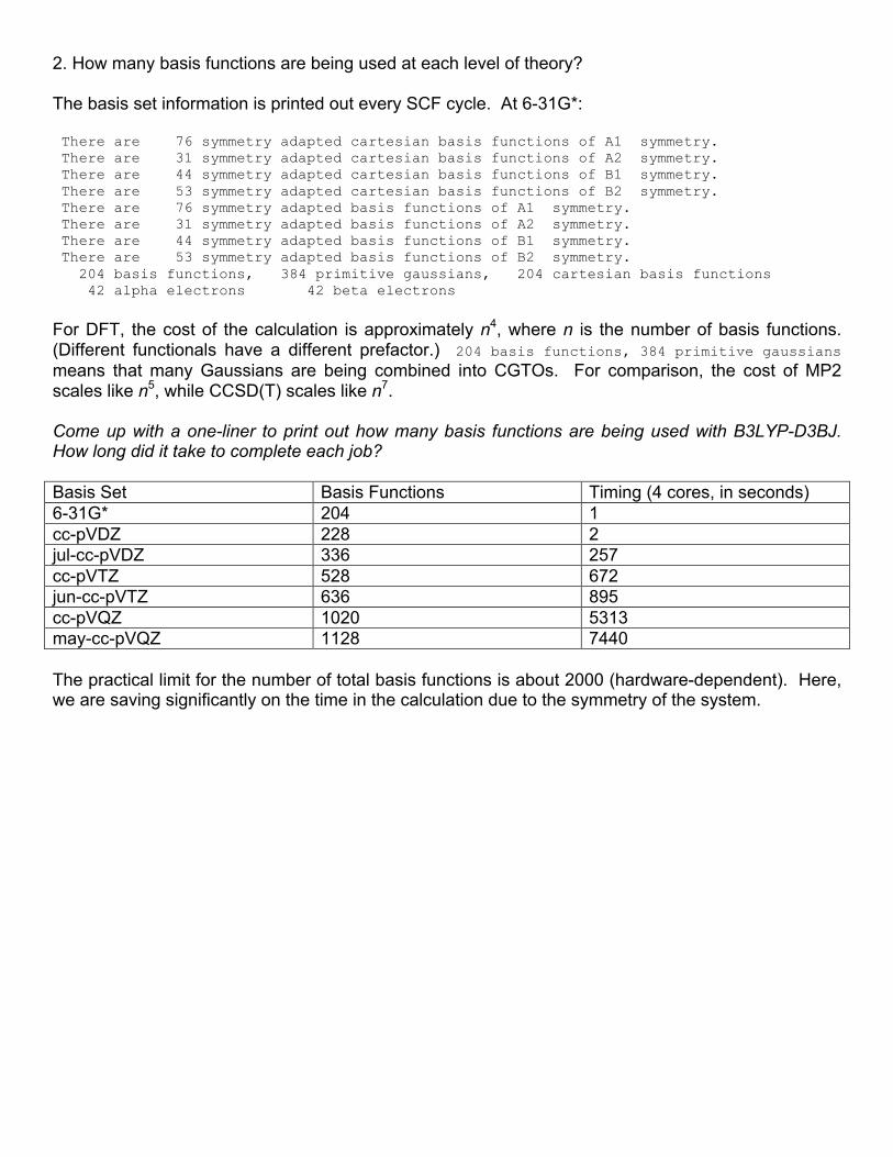
2. How many basis functions are being used at each level of theory? The basis set information is printed out every SCF cycle. At 6-31G*: There are 76 symmetry adapted cartesian basis functions of A1 symmetry. There are 31 symmetry adapted cartesian basis functions of A2 symmetry. There are 44 symmetry adapted cartesian basis functions of B1 symmetry. There are 53 symmetry adapted cartesian basis functions of B2 symmetry. There are 76 symmetry adapted basis functions of A1 symmetry. There are 31 symmetry adapted basis functions of A2 symmetry. There are 44 symmetry adapted basis functions of B1 symmetry. There are 53 symmetry adapted basis functions of B2 symmetry. 204 basis functions, 384 primitive gaussians, 204 cartesian basis functions 42 alpha electrons 42 beta electrons
For DFT, the cost of the calculation is approximately n4, where n is the number of basis functions. (Different functionals have a different prefactor.) 204 basis functions, 384 primitive gaussians means that many Gaussians are being combined into CGTOs. For comparison, the cost of MP2 scales like n5, while CCSD(T) scales like n7. Come up with a one-liner to print out how many basis functions are being used with B3LYP-D3BJ. How long did it take to complete each job? Basis Set Basis Functions Timing (4 cores, in seconds) 6-31G* 204 1 cc-pVDZ 228 2 jul-cc-pVDZ 336 257 cc-pVTZ 528 672 jun-cc-pVTZ 636 895 cc-pVQZ 1020 5313 may-cc-pVQZ 1128 7440 The practical limit for the number of total basis functions is about 2000 (hardware-dependent). Here, we are saving significantly on the time in the calculation due to the symmetry of the system.

Conclusions/Advice All calculations are imperfect to some extent due to the limitations of available methods and time. Our task in studying any particular problem is to choose a method that is informative and gives results in reasonable time. This is generally possible for many problems in organic chemistry. 1. Anchor to experiment. If you can’t anchor to experiment, anchor to ab initio in small model systems. (Approximate coupled cluster methods and composite methods can be applied to medium-sized systems.) 2. Just because a given model chemistry works for system A does not mean it will work for system B. PDDG is fine for alkane geometries, but will not give good barrier heights. 3. Modern DFTs are often heavily fitted to big experimental datasets, so it is quite possible for them to get the right answer for the wrong reasons. There is no systematic way to approach the right answer in DFT. 4. In contrast, performing CC calculations with big basis sets does systematically approach the right answer. It is simply very expensive. 5. Many computational methods are misused (B3LYP/6-31G*). Read the literature to understand the systems in which a given method is appropriate. What is the strength of the evidence to say that method X is appropriate for situation Y? 6. Dispersion corrections are obligatory (and cost essentially nothing extra). 7. Study the basis set convergence properties of your system. Are diffuse functions needed?
Eugene Kwan March 2017


![arXiv:1609.08947v2 [cond-mat.supr-con] 18 Nov 2016Figure 1. (Color online)(a) Crystal structure of) -BiPd (left), 3D Brillouin zone (top right) and 2D Brillouin zone (bottom right)](https://static.fdocument.org/doc/165x107/5f40a574b501eb25d22ead94/arxiv160908947v2-cond-matsupr-con-18-nov-2016-figure-1-color-onlinea-crystal.jpg)