Chapter 7 Specification: Choosing a Functional Form Copyright © 2011 Pearson Addison-Wesley. All...

Chapter 7

Specification: Choosing a

Functional Form

Copyright © 2011 Pearson Addison-Wesley.All rights reserved.

Slides by Niels-Hugo BlunchWashington and Lee University

7-2 © 2011 Pearson Addison-Wesley. All rights reserved.

The Use and Interpretation of the Constant Term

• An estimate of β0 has at least three components:

1. the true β0

2. the constant impact of any specification errors (an omitted variable, for example)

3. the mean of ε for the correctly specified equation (if not equal to zero)

• Unfortunately, these components can’t be distinguished from one another because we can observe only β0, the sum of the three components

• As a result of this, we usually don’t interpret the constant term

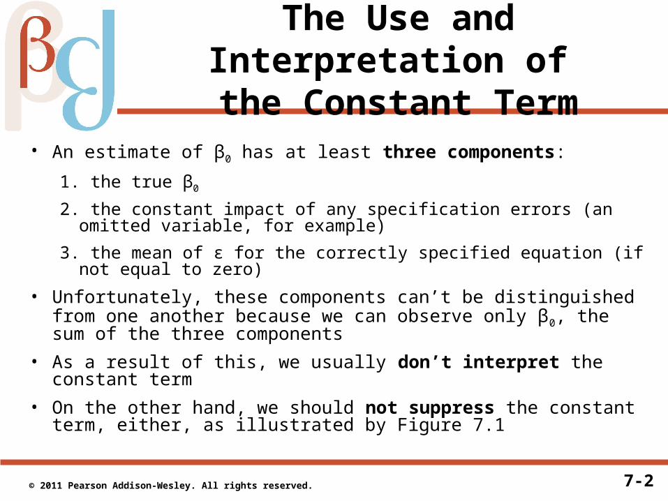
• On the other hand, we should not suppress the constant term, either, as illustrated by Figure 7.1


Figure 7.1 The Harmful Effect of Suppressing the Constant Term


Alternative Functional Forms

• An equation is linear in the variables if plotting the function in terms of X and Y generates a straight line

• For example, Equation 7.1:

Y = β0 + β1X + ε (7.1)

is linear in the variables but Equation 7.2:

Y = β0 + β1X2 + ε (7.2)

is not linear in the variables

• Similarly, an equation is linear in the coefficients only if the coefficients appear in their simplest form—they:

– are not raised to any powers (other than one)

– are not multiplied or divided by other coefficients

– do not themselves include some sort of function (like logs or exponents)


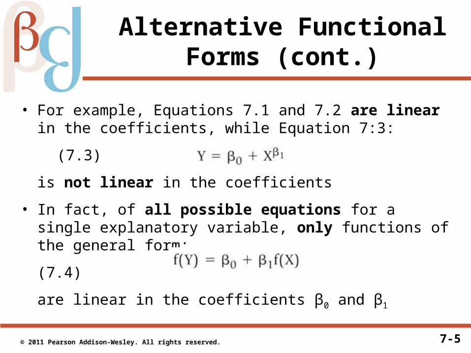
• For example, Equations 7.1 and 7.2 are linear in the coefficients, while Equation 7:3:

(7.3)

is not linear in the coefficients

• In fact, of all possible equations for a single explanatory variable, only functions of the general form:

(7.4)

are linear in the coefficients β0 and β1

Alternative Functional Forms (cont.)


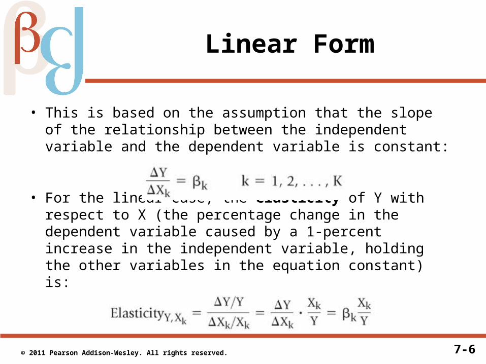
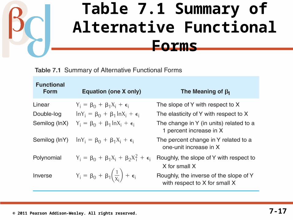
Linear Form

• This is based on the assumption that the slope of the relationship between the independent variable and the dependent variable is constant:

• For the linear case, the elasticity of Y with respect to X (the percentage change in the dependent variable caused by a 1-percent increase in the independent variable, holding the other variables in the equation constant) is:


What Is a Log?

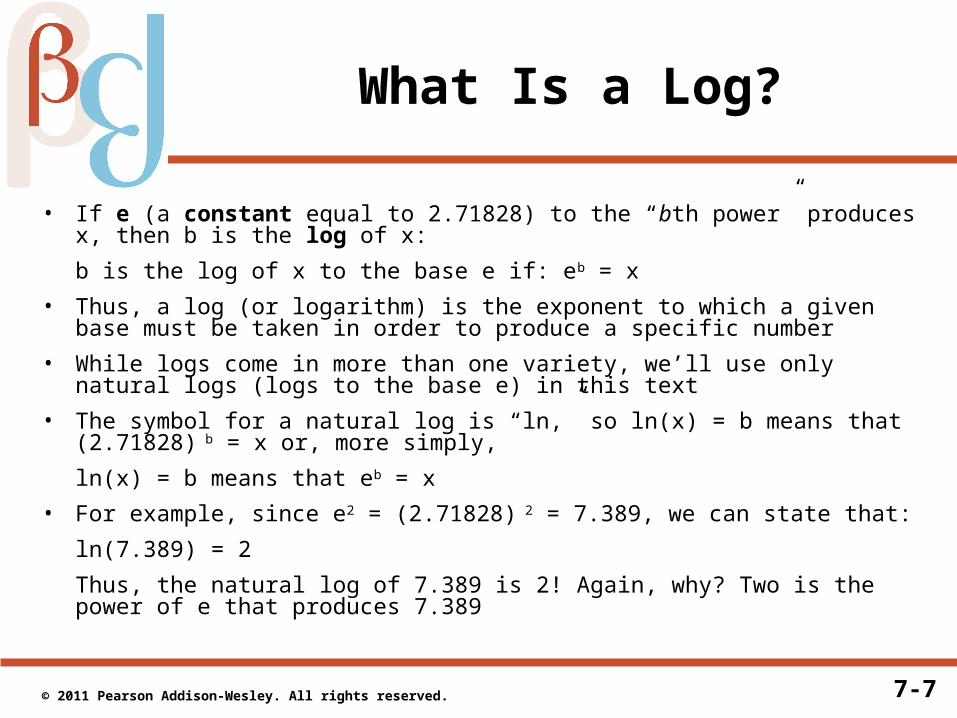
• If e (a constant equal to 2.71828) to the “bth power” produces x, then b is the log of x:

b is the log of x to the base e if: eb = x

• Thus, a log (or logarithm) is the exponent to which a given base must be taken in order to produce a specific number

• While logs come in more than one variety, we’ll use only natural logs (logs to the base e) in this text

• The symbol for a natural log is “ln,” so ln(x) = b means that (2.71828) b = x or, more simply,

ln(x) = b means that eb = x

• For example, since e2 = (2.71828) 2 = 7.389, we can state that:

ln(7.389) = 2

Thus, the natural log of 7.389 is 2! Again, why? Two is the power of e that produces 7.389


What Is a Log? (cont.)

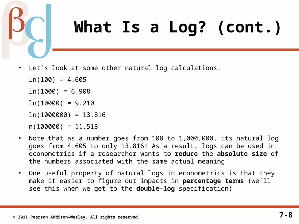
• Let’s look at some other natural log calculations:

ln(100) = 4.605

ln(1000) = 6.908

ln(10000) = 9.210

ln(1000000) = 13.816

n(100000) = 11.513

• Note that as a number goes from 100 to 1,000,000, its natural log goes from 4.605 to only 13.816! As a result, logs can be used in econometrics if a researcher wants to reduce the absolute size of the numbers associated with the same actual meaning

• One useful property of natural logs in econometrics is that they make it easier to figure out impacts in percentage terms (we’ll see this when we get to the double-log specification)


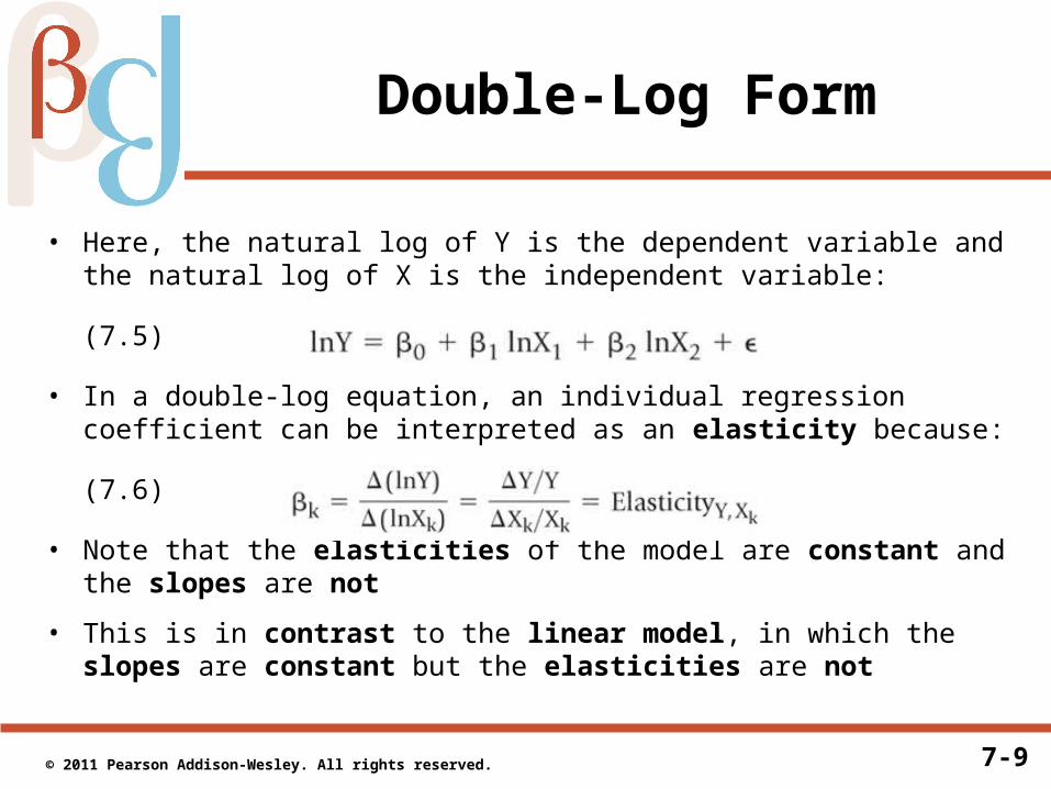
Double-Log Form

• Here, the natural log of Y is the dependent variable and the natural log of X is the independent variable:

(7.5)

• In a double-log equation, an individual regression coefficient can be interpreted as an elasticity because:

(7.6)

• Note that the elasticities of the model are constant and the slopes are not

• This is in contrast to the linear model, in which the slopes are constant but the elasticities are not


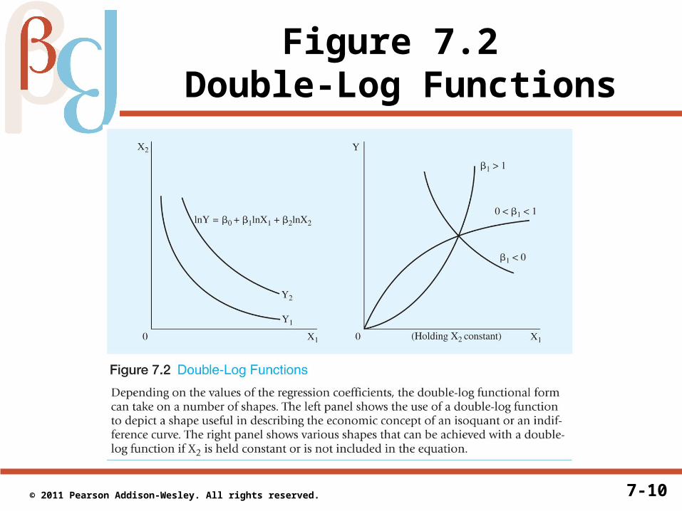
Figure 7.2 Double-Log Functions


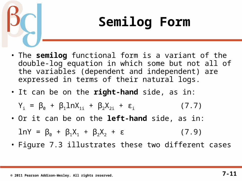
Semilog Form

• The semilog functional form is a variant of the double-log equation in which some but not all of the variables (dependent and independent) are expressed in terms of their natural logs.

• It can be on the right-hand side, as in:

Yi = β0 + β1lnX1i + β2X2i + εi (7.7)

• Or it can be on the left-hand side, as in:

lnY = β0 + β1X1 + β2X2 + ε (7.9)

• Figure 7.3 illustrates these two different cases


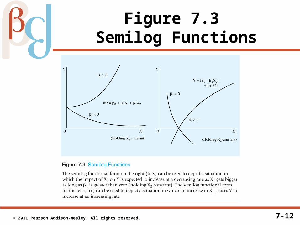
Figure 7.3 Semilog Functions


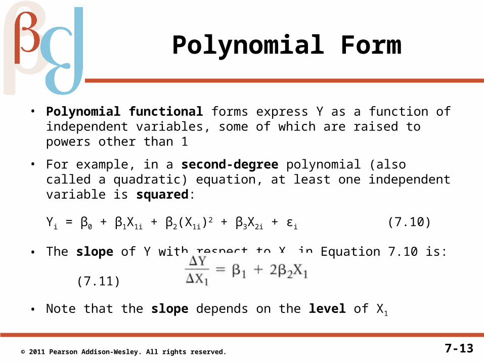
Polynomial Form

• Polynomial functional forms express Y as a function of independent variables, some of which are raised to powers other than 1

• For example, in a second-degree polynomial (also called a quadratic) equation, at least one independent variable is squared:

Yi = β0 + β1X1i + β2(X1i)2 + β3X2i + εi (7.10)

• The slope of Y with respect to X1 in Equation 7.10 is:

(7.11)

• Note that the slope depends on the level of X1


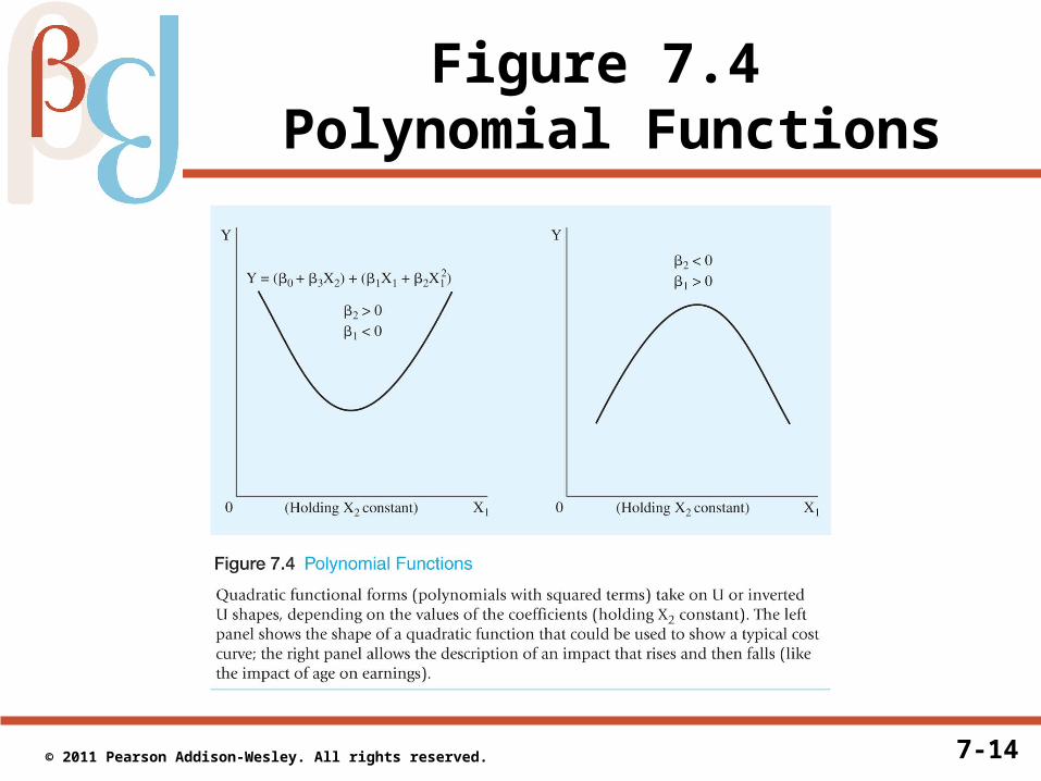
Figure 7.4 Polynomial Functions


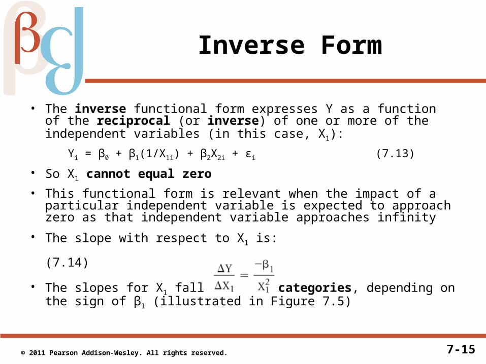
Inverse Form

• The inverse functional form expresses Y as a function of the reciprocal (or inverse) of one or more of the independent variables (in this case, X1):

Yi = β0 + β1(1/X1i) + β2X2i + εi (7.13)

• So X1 cannot equal zero

• This functional form is relevant when the impact of a particular independent variable is expected to approach zero as that independent variable approaches infinity

• The slope with respect to X1 is:

(7.14)

• The slopes for X1 fall into two categories, depending on the sign of β1 (illustrated in Figure 7.5)


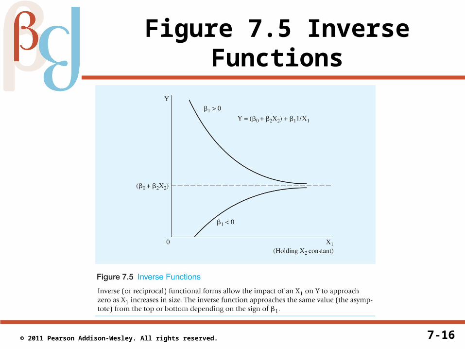
Figure 7.5 Inverse Functions


Table 7.1 Summary of Alternative Functional Forms


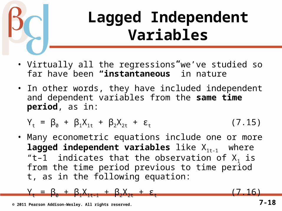
Lagged Independent Variables

• Virtually all the regressions we’ve studied so far have been “instantaneous” in nature

• In other words, they have included independent and dependent variables from the same time period, as in:

Yt = β0 + β1X1t + β2X2t + εt (7.15)

• Many econometric equations include one or more lagged independent variables like X1t-1 where “t–1” indicates that the observation of X1 is from the time period previous to time period t, as in the following equation:

Yt = β0 + β1X1t-1 + β2X2t + εt (7.16)


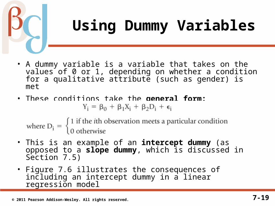
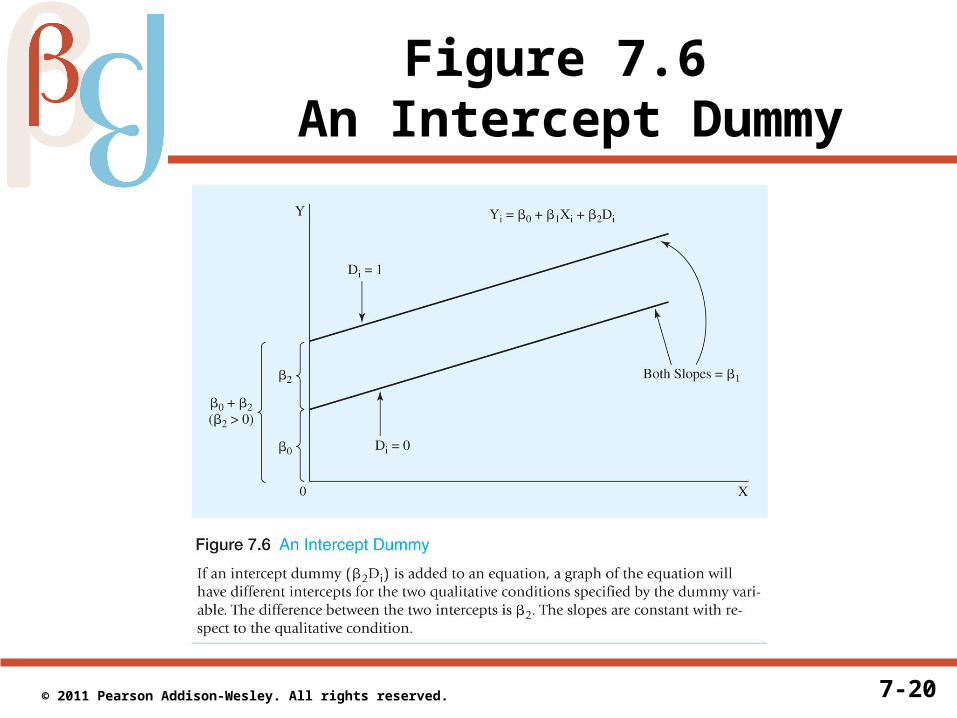
Using Dummy Variables

• A dummy variable is a variable that takes on the values of 0 or 1, depending on whether a condition for a qualitative attribute (such as gender) is met

• These conditions take the general form:

(7.18)

• This is an example of an intercept dummy (as opposed to a slope dummy, which is discussed in Section 7.5)

• Figure 7.6 illustrates the consequences of including an intercept dummy in a linear regression model


Figure 7.6 An Intercept Dummy


Slope Dummy Variables

• Contrary to the intercept dummy, which changed only the intercept (and not the slope), the slope dummy changes both the intercept and the slope

• The general form of a slope dummy equation is:

Yi = β0 + β1Xi + β2Di + β3XiDi + εi

(7.20)

• The slope depends on the value of D:

When D = 0, ΔY/ΔX = β1

When D = 1, ΔY/ΔX = (β1 + β3)

• Graphical illustration of how this works in Figure 7.7


Figure 7.7 Slope and Intercept Dummies


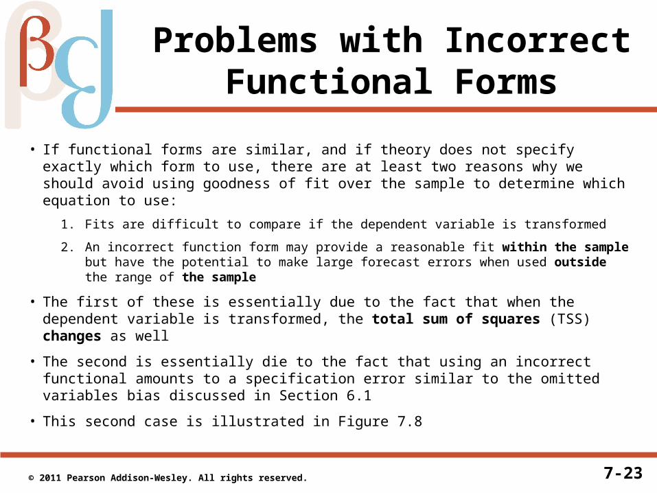
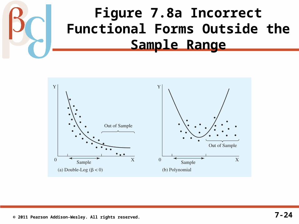
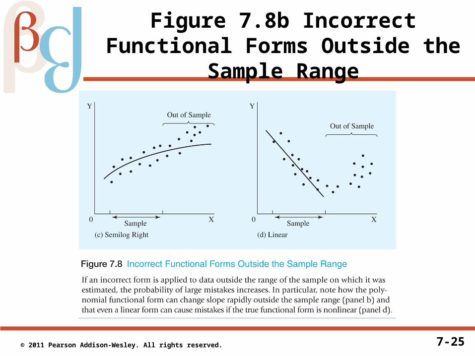
Problems with Incorrect Functional Forms

• If functional forms are similar, and if theory does not specify exactly which form to use, there are at least two reasons why we should avoid using goodness of fit over the sample to determine which equation to use:

1. Fits are difficult to compare if the dependent variable is transformed

2. An incorrect function form may provide a reasonable fit within the sample but have the potential to make large forecast errors when used outside the range of the sample

• The first of these is essentially due to the fact that when the dependent variable is transformed, the total sum of squares (TSS) changes as well

• The second is essentially die to the fact that using an incorrect functional amounts to a specification error similar to the omitted variables bias discussed in Section 6.1

• This second case is illustrated in Figure 7.8


Figure 7.8a Incorrect Functional Forms Outside the Sample Range


Figure 7.8b Incorrect Functional Forms Outside the Sample Range


Key Terms from Chapter 7

• Elasticity

• Double-log functional form

• Semilog functional form

• Polynomial functional form

• Inverse functional form

• Slope dummy

• Natural log

• Omitted condition

• Interaction term

• Linear in the variables

• Linear in the coefficients

Chapter 7 Specification: Choosing a Functional Form Copyright © 2011 Pearson Addison-Wesley. All...

Documents

Transcript of Chapter 7 Specification: Choosing a Functional Form Copyright © 2011 Pearson Addison-Wesley. All...