1ti` +iBQMQ7: BiS ii2`Mb7`QK aK `iT?QM2@ …tesi.cab.unipd.it/54371/1/Lanaro_Alberto_Tesi.pdf · M...
127
Transcript of 1ti` +iBQMQ7: BiS ii2`Mb7`QK aK `iT?QM2@ …tesi.cab.unipd.it/54371/1/Lanaro_Alberto_Tesi.pdf · M...


τ
ht


1
1.1 Human Activity Recognition
1.1.1 Sensors
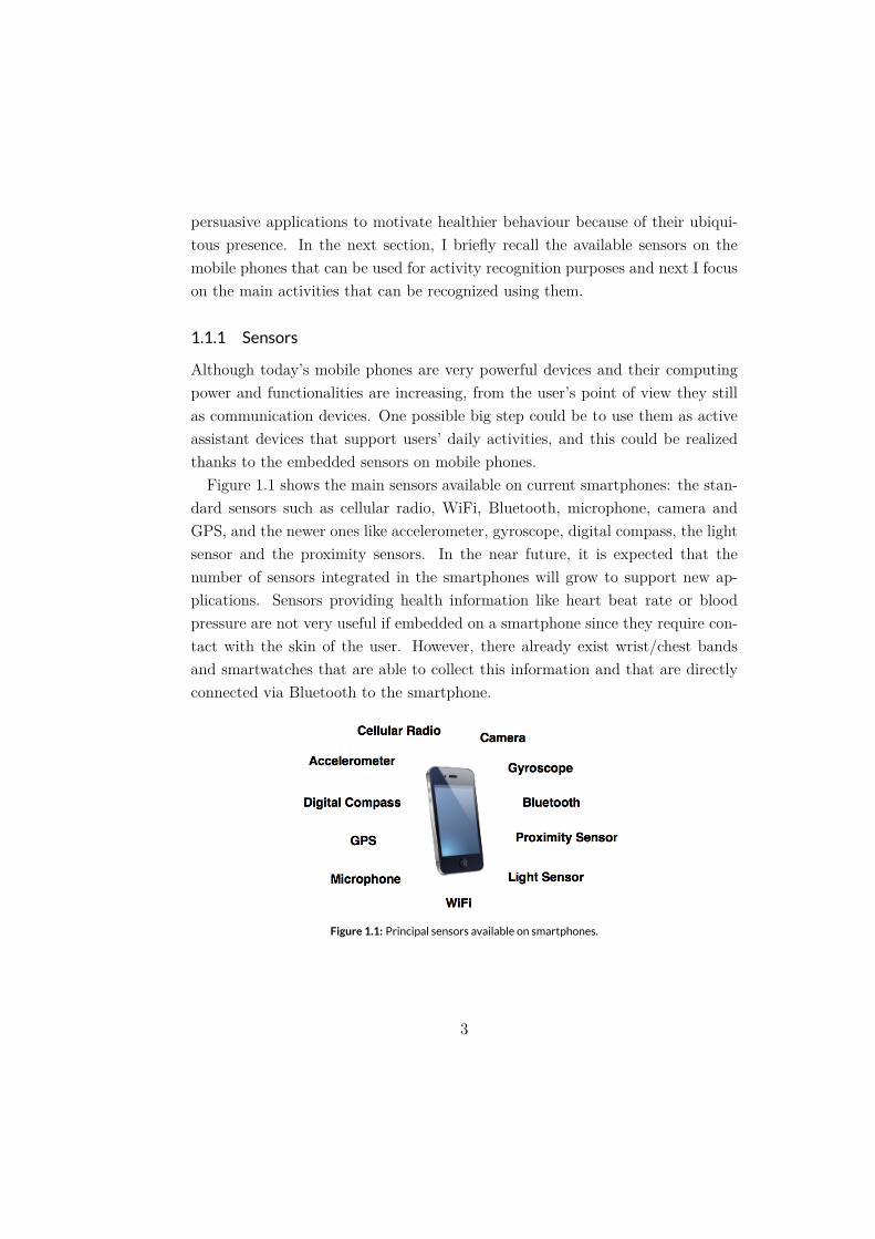
Figure 1.1: Principal sensors available on smartphones.
1.1.2 Activities and Applications
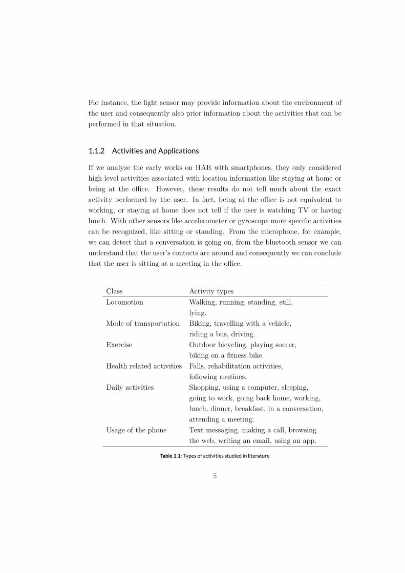
Table 1.1: Types of activities studied in literature
1.1.3 Activity Recognition Process
Activity Classification Steps
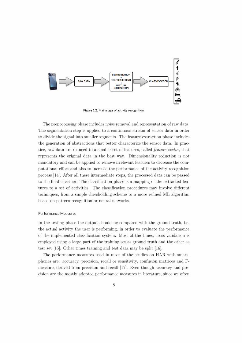
Figure 1.2:Main steps of activity recognition.
PerformanceMeasures
1.1.4 Challenges of Activity Recognition with Smartphones
Continuous Sensing
Running Classifiers on Smartphones
Phone Context Problem
Training Burden
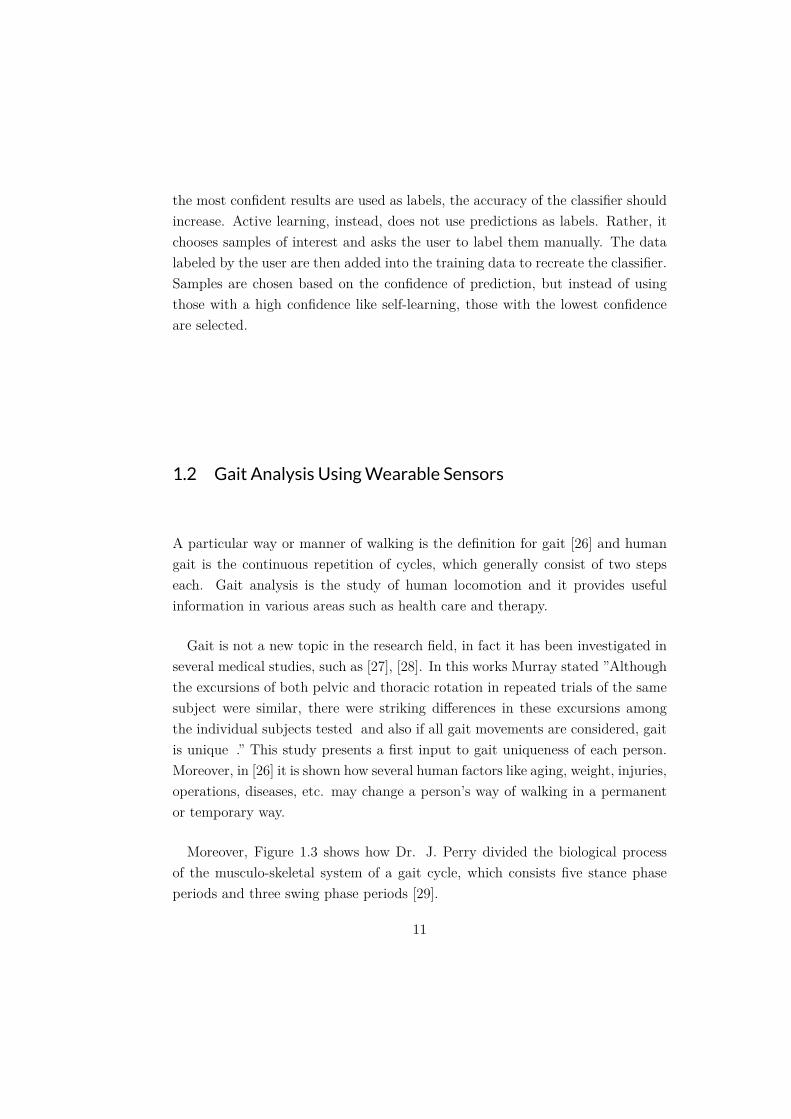
1.2 Gait Analysis UsingWearable Sensors
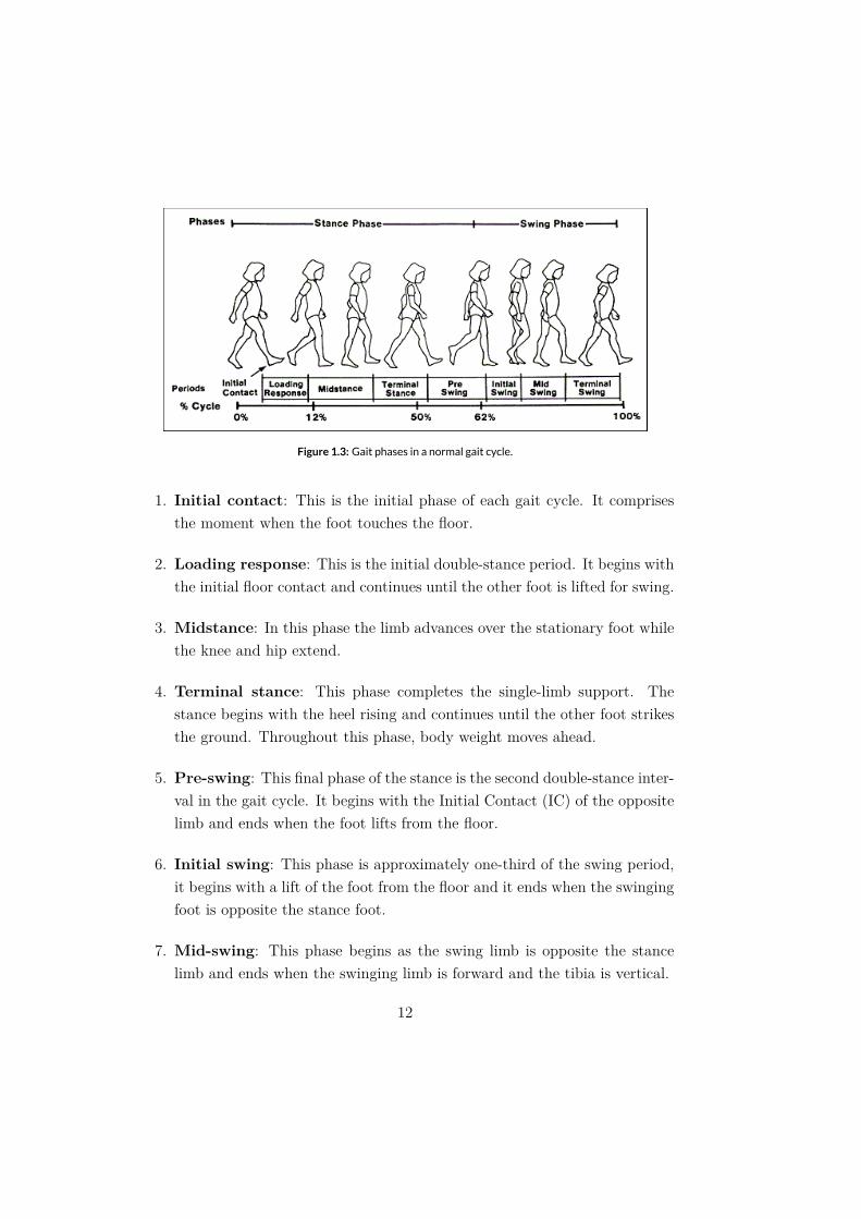
Figure 1.3: Gait phases in a normal gait cycle.

1.3 Gait Identification
1.4 Motivations and Contributions
2
5.45%

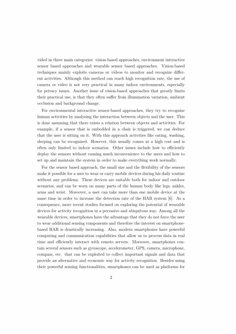
33.1 Computer Vision
3.2 Camera Calibration
3.2.1 CameraModel
R C f
C RR
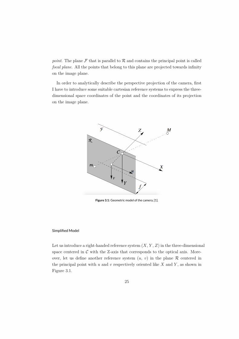
F R
Figure 3.1: Geometric model of the camera, [1].
SimplifiedModel
X Y Z
Cu v R
u v X Y
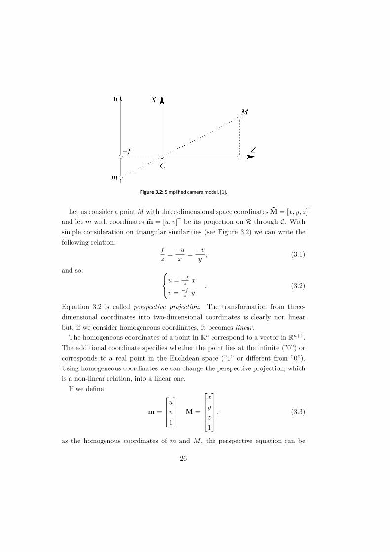
Figure 3.2: Simplified cameramodel, [1].
M M̃ = [x, y, z]⊤
m m̃ = [u, v]⊤ R C
f
z=−ux
=−vy
,
⎧⎨
⎩u = −f
z x
v = −fz y
.
Rn Rn+1
m =
⎡
⎢⎣u
v
1
⎤
⎥⎦ M =
⎡
⎢⎢⎢⎣
x
y
z
1
⎤
⎥⎥⎥⎦,
m M
z
⎡
⎢⎣u
v
1
⎤
⎥⎦ =
⎡
⎢⎣−fx−fyz
⎤
⎥⎦ =
⎡
⎢⎣−f 0 0 0
0 −f 0 0
0 0 1 0
⎤
⎥⎦
⎡
⎢⎢⎢⎣
x
y
z
1
⎤
⎥⎥⎥⎦.
zm = PM,
m ≃ PM,
≃ z P
GeneralModel
Intrinsic parameters
u
v ⎧⎨
⎩u = ku
−fz x+ u0
v = kv−fz y + v0 ,
u0 v0 ku kvu v pixel ·m−1
P =
⎡
⎢⎣−fku 0 u0 0
0 −fkv v0 0
0 0 1 0
⎤
⎥⎦ = K[I|0],
K =
⎡
⎢⎣−fku 0 u0
0 −fkv v00 0 1
⎤
⎥⎦ .
Extrinsic parameters
R t Mc
M
Mc = GM,
G =
[R t
0 1
].
m ≃ K[I|0]Mc = K[I|0]GM,
P = K[I|0]G.
G
K
[I|0]
P = K[R|t].
Normalized Coordinates
p = K−1m,
[I|0]
Scaling Factor
P γP
∀γ ∈ R \ {0}
Degrees of Freedom
P
3.2.2 Calibration
3.3 Optical Flow
I(x, t) = I(x+ v∆t, t+∆t)
I(x, t)
I(x+ v∆t, t+∆t) = I(x, t) + gradI(x, t)⊤[v∆t
∆t
].
I(x+ v∆t, t+∆t) = I(x, t) +∇I(x, t)⊤v∆t+ It(x, t)∆t,
∇I ( ∂I∂x ,∂I∂y )
⊤ ItI
∆t
∇I(x, t)⊤v + It(x, t) = 0.
(v) = (vx, vy)
∇I(x, t)⊤v
3.3.1 Optical Flow Estimation
Lucas and Kanade
v n × n
v xi ∈ W
∇I(xi, t)⊤v = −It(xi, t).
n× n
Av = b
A =
⎡
⎢⎣∇I(x1, t)⊤
∇I(xn×n, t)⊤
⎤
⎥⎦ b =
⎡
⎢⎣−It(x1, t)
−It(xn×n, t)
⎤
⎥⎦
v = A−1b = (A⊤A)−1A⊤b.
w(xi) W
Kanade, Lucas and Tomasi Feature Tracker
λmax/λmin ≃ 1 λmax λmin
min(λ1,λ2) > λth,
λth λmin
λmax
InputOutput
I(t) I(t+ 1)
I(t) v n × n
I(t+ 1)
3.3.2 Keypoints Extraction
SIFT
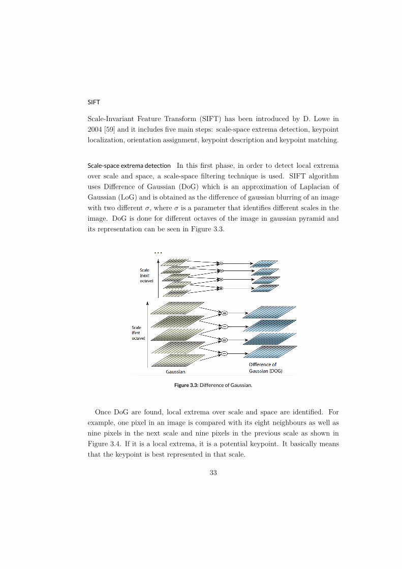
Scale-space extrema detection
σ σ
Figure 3.3: Difference of Gaussian.
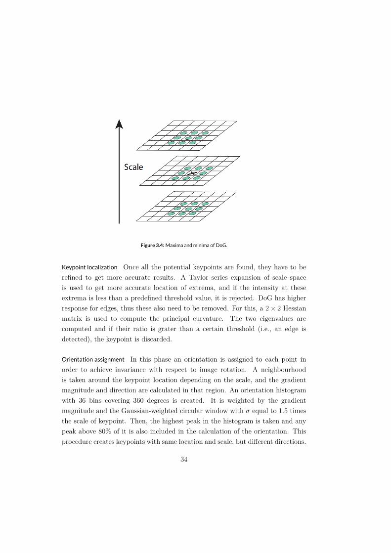
Figure 3.4:Maxima andminima of DoG.
Keypoint localization
2× 2
Orientation assignment
σ
Keypoint description 16×164×4
Keypointmatching
3.4 Motion and Structure
3.4.1 Essential Matrix
P P ′
p = K−1m p′ = K ′−1m′
P = [I|0] and P ′ = [I|0]G = [R|t]
p′⊤[t]×Rp = 0 .
E ! [t]×R,
det[t]× = 0
E
3.4.2 Essential Matrix Factorization
R U V
det(UV ⊤)URV ⊤
3 × 3 E
E = SR R S
S = [t]× ∥t∥ = 1 U Ut = [0, 0, 1]⊤ ! a
S = [t]× = [U⊤a]×
S = [U⊤a]× = U⊤[a]×U.
a ∈ R
[a]× !
⎡
⎣0 −a3 a2a3 0 −a1−a2 a1 0
⎤
⎦ ,
[a]×b = a× b
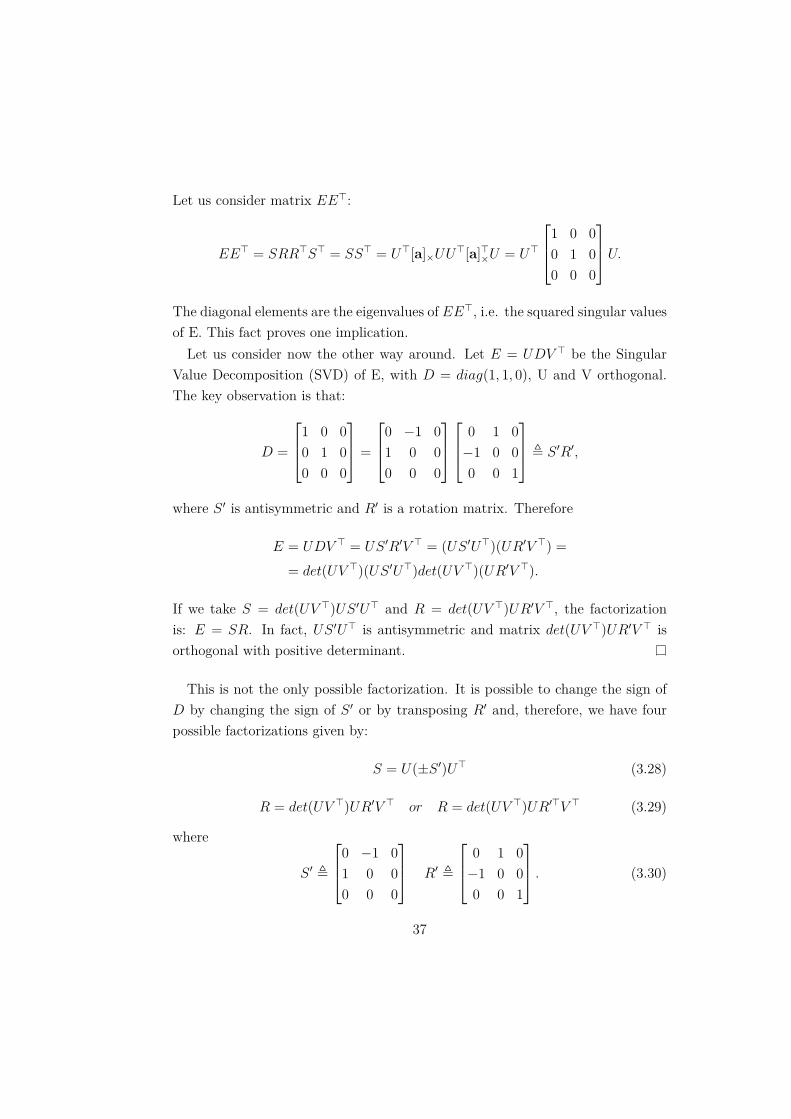
EE⊤
EE⊤ = SRR⊤S⊤ = SS⊤ = U⊤[a]×UU⊤[a]⊤×U = U⊤
⎡
⎢⎣1 0 0
0 1 0
0 0 0
⎤
⎥⎦U.
EE⊤
E = UDV ⊤
D = diag(1, 1, 0)
D =
⎡
⎢⎣1 0 0
0 1 0
0 0 0
⎤
⎥⎦ =
⎡
⎢⎣0 −1 0
1 0 0
0 0 0
⎤
⎥⎦
⎡
⎢⎣0 1 0
−1 0 0
0 0 1
⎤
⎥⎦ ! S ′R′,
S ′ R′
E = UDV ⊤ = US ′R′V ⊤ = (US ′U⊤)(UR′V ⊤) =
= det(UV ⊤)(US ′U⊤)det(UV ⊤)(UR′V ⊤).
S = det(UV ⊤)US ′U⊤ R = det(UV ⊤)UR′V ⊤
E = SR US ′U⊤ det(UV ⊤)UR′V ⊤
D S ′ R′
S = U(±S ′)U⊤
R = det(UV ⊤)UR′V ⊤ or R = det(UV ⊤)UR′⊤V ⊤
S ′ !
⎡
⎢⎣0 −1 0
1 0 0
0 0 0
⎤
⎥⎦ R′ !
⎡
⎢⎣0 1 0
−1 0 0
0 0 1
⎤
⎥⎦ .
3.4.3 Essential Matrix Computation
{(pi,p⊤i )|i = 1, · · · , n}
p⊤i Epi = 0.
vec
p′⊤i Epi = 0⇐⇒ vec(p′⊤
i Epi) = 0⇐⇒ (p⊤i ⊗ p′⊤
i )vec(E) = 0.
n
n
⎡
⎢⎢⎢⎢⎣
p⊤1 ⊗ p⊤′
1
p⊤2 ⊗ p⊤′
2
p⊤n ⊗ p⊤′
n
⎤
⎥⎥⎥⎥⎦
︸ ︷︷ ︸Un
vec(E) = 0.
Un n = 8
m× n A vec(A) mn× 1
A m×n B p× qA B mp× nq
A⊗B =
⎡
⎢⎣a11B . . . a1nB
am1B . . . amnB
⎤
⎥⎦ .

U⊤n Un
Un

44.1 Unsupervised Learning
Y = (Y1, . . . , Ym)
X = (X1, . . . , Xp) xi = (xi1, . . . , xip) i
yi(x1, y1), . . . , (xn, yn)
(X, Y )
P (X, Y )
P (Y |X)
µ x
µ(x) = argminθ
EY |XL(Y, θ),
L(Y, θ)
P (X, Y ) = P (Y |X) · P (X),
P (X) X
P (X)
P (Y |X) Y
µ(x)
N
(x1, x2, . . . , xn) p X P (X)
X
X
P (X)
P (X)
P (x)
X
P (X)
X
P (X)
P (X)
P (X, Y )
4.2 Unsupervised Clustering
4.2.1 A Taxonomy of ClusteringMethods
[0, 1] {0, 1}
Partitional clustering
Hierarchical clustering.
4.2.2 Cluster Validity Analysis
4.3 Growing Neural Gas
Rn
Rn
ξ
4.3.1 GNGPseudo-code
k
wk Rn
errork
k
INIT
ξ
s t ξ
ws wt ∥ws − ξ∥∥wt − ξ∥ k
s
ws ξ errors
errors ← errors + ∥ws − ξ∥ ,
s s
ξ ew en ew, en ∈ [0, 1]
ws ← ws + ew(ξ −ws),
wn ← wn + en(ξ −wn), ∀n ∈ Neighbours(s).
s
s t
amax
λ
r
u
u v
r u v
wr ←(wu +wv)
2.
u r v r
u v
u v
erroru ← α× erroru,
errorv ← α× errorv,
errorr ← erroru.
j β
errorj ← β × errorj.
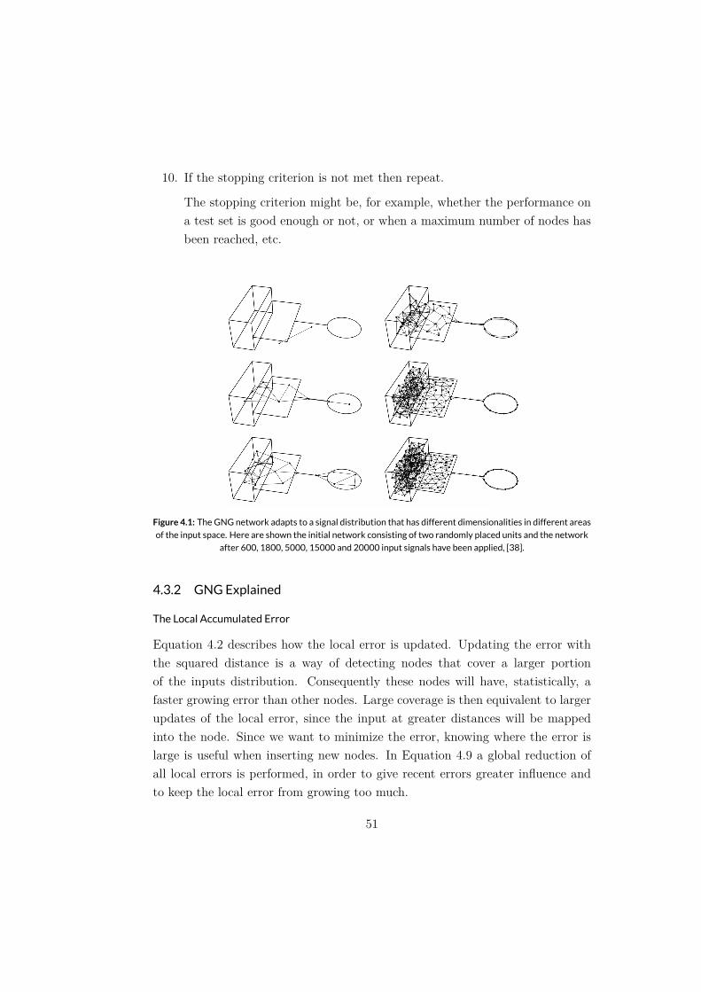
Figure 4.1: TheGNG network adapts to a signal distribution that has different dimensionalities in different areas
of the input space. Here are shown the initial network consisting of two randomly placed units and the network
after 600, 1800, 5000, 15000 and 20000 input signals have been applied, [38].
4.3.2 GNGExplained
The Local Accumulated Error
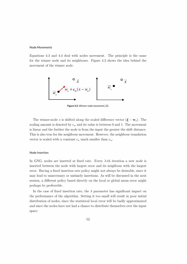
NodeMovements
Figure 4.2:Winner nodemovement, [2].
s (ξ −ws)
ew
en ew
Node Insertion
λ
λ
4.4 The GrowingWhen Required Network
4.4.1 GNG vs. GWR
4.4.2 GWRPseudo-code
A
C ⊆ A × A
p(ξ) ξ wn n
INIT
A = {n1, n2},
n1 n2 p(ξ)
C = ∅.
ξ
i
∥ξ −wi∥
s, t ∈ A
s = argminn∈A
∥ξ −wn∥
t = argminn∈A\{s}
∥ξ −wn∥ ,
wn n
s t
C = C ∪ {(s, t)},
a = exp(−∥ξ −ws∥).
a < atht
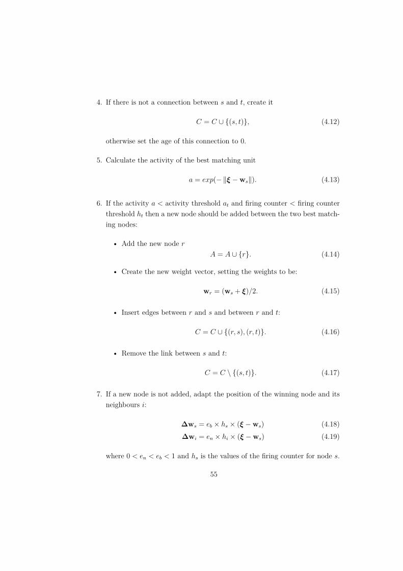
r
A = A ∪ {r}.
wr = (ws + ξ)/2.
r s r t
C = C ∪ {(r, s), (r, t)}.
s t
C = C \ {(s, t)}.
i
∆ws = eb × hs × (ξ −ws)
∆wi = en × hi × (ξ −ws)
0 < en < eb < 1 hs s
s
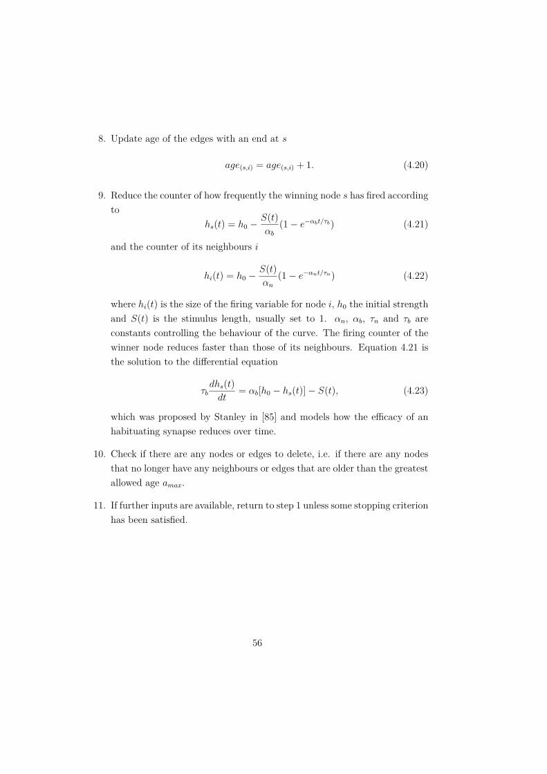
age(s,i) = age(s,i) + 1.
s
hs(t) = h0 −S(t)
αb(1− e−αbt/τb)
i
hi(t) = h0 −S(t)
αn(1− e−αnt/τn)
hi(t) i h0
S(t) αn αb τn τb
τbdhs(t)
dt= αb[h0 − hs(t)]− S(t),
amax
5
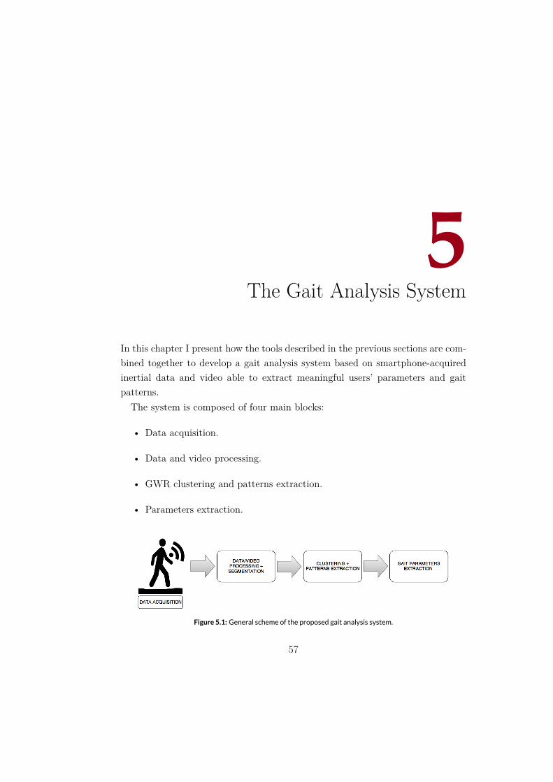
Figure 5.1: General scheme of the proposed gait analysis system.
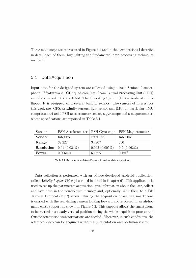
5.1 Data Acquisition
Table 5.1: IMU specifics of Asus Zenfone 2 used for data acquisition.
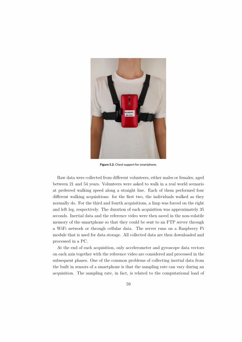
Figure 5.2: Chest support for smartphone.
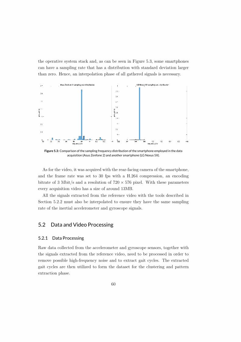
Figure 5.3: Comparison of the sampling frequency distribution of the smartphone employed in the data
acquisition (Asus Zenfone 2) and another smartphone (LGNexus 5X).
720 × 576
5.2 Data and Video Processing
5.2.1 Data Processing
Interpolation
fs = 200
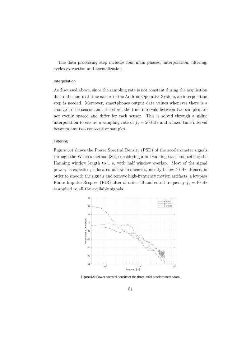
Filtering
fc = 40
100 101 102
frequency [Hz]
-50
-40
-30
-20
-10
0
10
20
30
Po
we
r S
pe
ctra
l De
nsi
ty [
dB
]
x-axis acc
y-axis acc
z-axis acc
Figure 5.4: Power spectral density of the three-axial accelerometer data.
10 10.5 11 11.5 12 12.5 13 13.5 14time [s]
4
6
8
10
12
14
16
18
m/s
2
Original signalFiltered signal
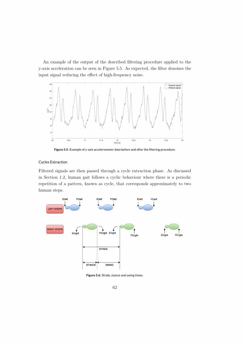
Figure 5.5: Example of y-axis accelerometer data before and after the filtering procedure.
Cycles Extraction
Figure 5.6: Stride, stance and swing times.
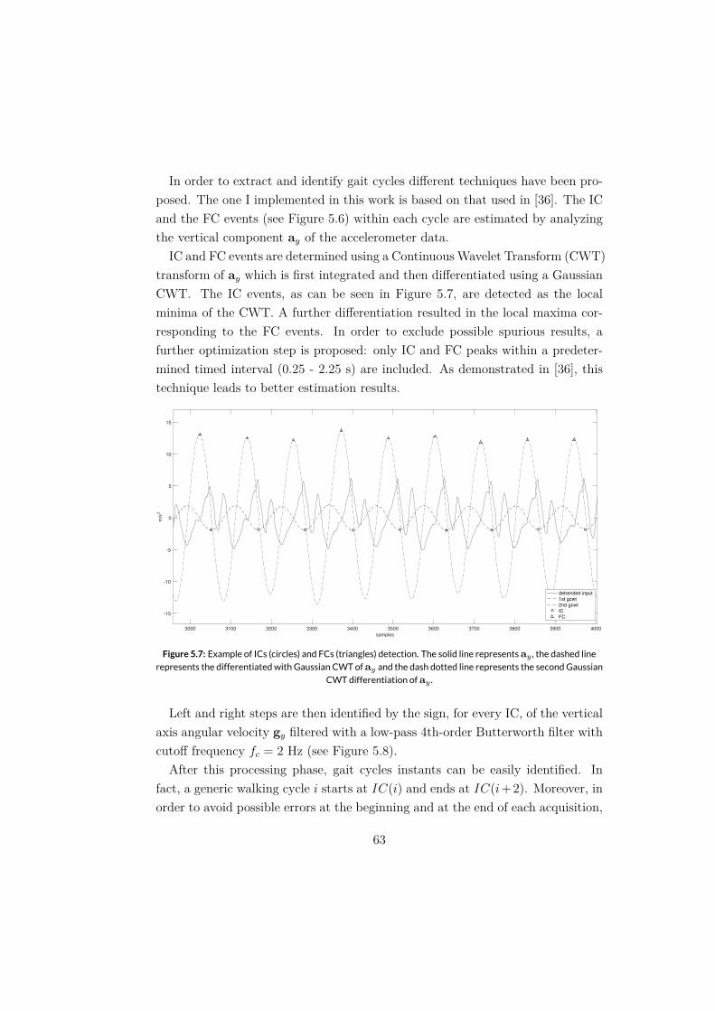
ay
ay
3000 3100 3200 3300 3400 3500 3600 3700 3800 3900 4000samples
-15
-10
-5
0
5
10
15
m/s
2
detrended input1st gcwt2nd gcwtICFC
Figure 5.7: Example of ICs (circles) and FCs (triangles) detection. The solid line representsay , the dashed linerepresents the differentiatedwith Gaussian CWT ofay and the dash dotted line represents the secondGaussian
CWT differentiation ofay .
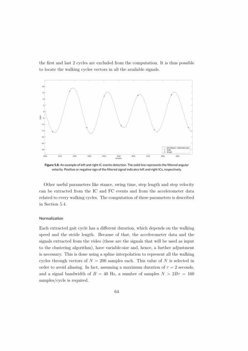
gy
fc = 2
i IC(i) IC(i+2)
3000 3100 3200 3300 3400 3500 3600 3700 3800 3900samples
-30
-25
-20
-15
-10
-5
0
5
10
15
20
deg/
s
2Hz-filtered + detrended inputICleftICright
Figure 5.8: An example of left and right IC events detection. The solid line represents the filtered angular
velocity. Positive or negative sign of the filtered signal indicates left and right ICs, respectively.
Normalization
N = 200 N
τ = 2
B = 40 N > 2Bτ = 160
5.2.2 Video Processing
OpenCV-Python
C++
C++
C/C++
C/C++ C/C++
Problem Formulation
Input
t t+ 1 It It+1
Output R
t
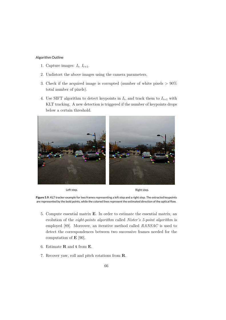
AlgorithmOutline
It It+1
It It+1
Left step. Right step.
Figure 5.9: KLT tracker example for two frames representing a left step and a right step. The extracted keypoints
are represented by the bold points, while the colored lines represent the estimated direction of the optical flow.
E
E
R t E
R
RANSAC
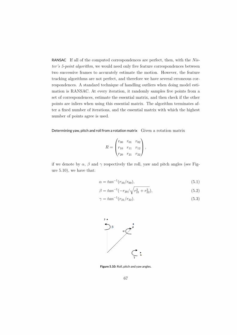
Determining yaw, pitch and roll from a rotationmatrix
R =
⎛
⎜⎝r00 r01 r02r10 r11 r12r20 r21 r22
⎞
⎟⎠ ,
α β γ
α = tan−1(r10/r00),
β = tan−1(−r20/√
r221 + r222),
γ = tan−1(r21/r22).
Figure 5.10: Roll, pitch and yaw angles.
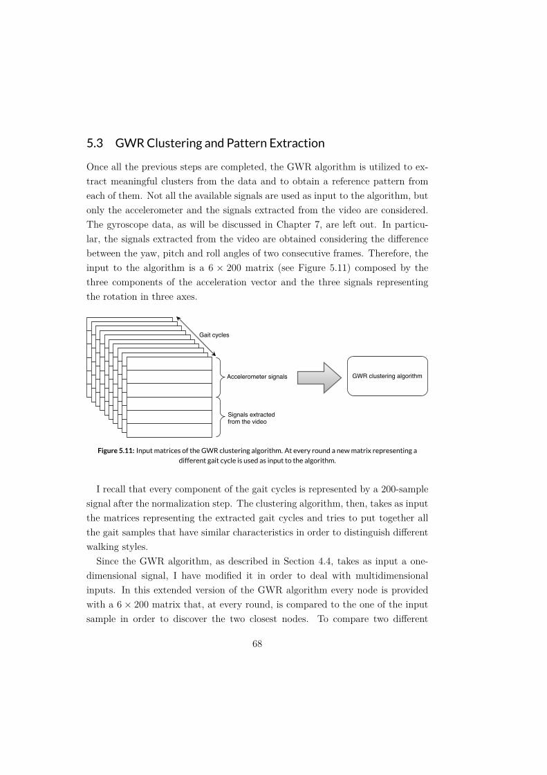
5.3 GWRClustering and Pattern Extraction
6 × 200
Figure 5.11: Input matrices of the GWR clustering algorithm. At every round a newmatrix representing a
different gait cycle is used as input to the algorithm.
6× 200
a× b I U d(I,U)
d(I,U) =
∑ai=1 ∥Ii −Ui∥
a,
Ii Ui I U
d(I,U)
5.3.1 GWRParameters
at ht
eb en
h0 S(t) αb αn τb τnh(t)
h0 = 1 S(t) = 1 αb = 1.05 αn = 1.05 τb = 3.33 τn = 14.3
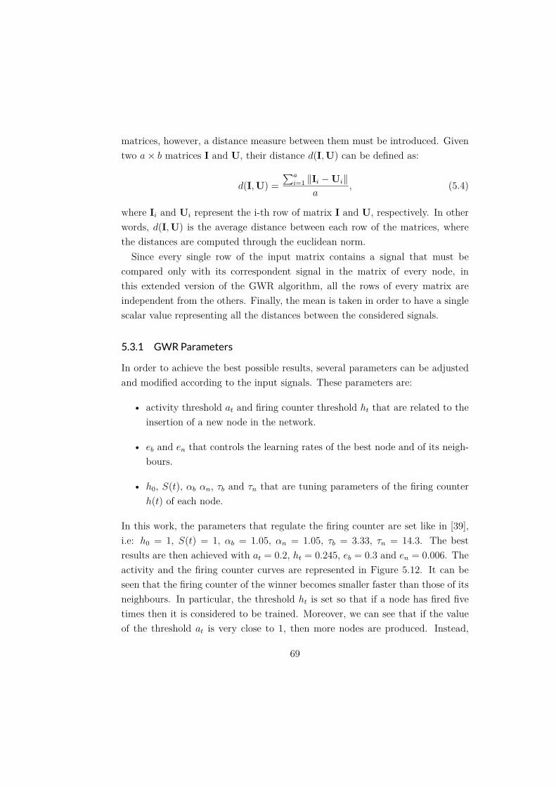
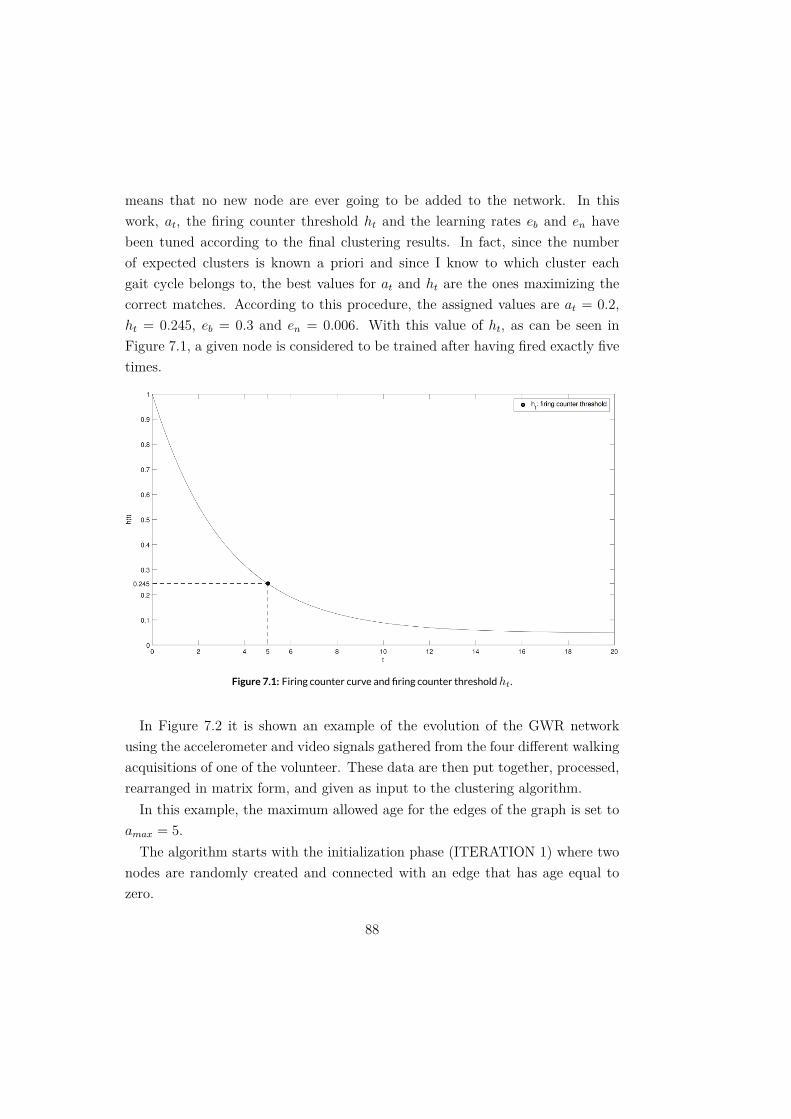
at = 0.2 ht = 0.245 eb = 0.3 en = 0.006
ht
at
at
0 2 4 6 8 10 12 14 16 18 20
|| ξ - w||
0
0.1
0.2
0.3
0.4
0.5
0.6
0.7
0.8
0.9
1
e|| ξ
- w
||
Activity curve
0 2 4 6 8 10 12 14 16 18 20
t
0
0.1
0.2
0.3
0.4
0.5
0.6
0.7
0.8
0.9
1
h(t
)
Firing counter curve for different values of τ
τ = 3.33τ = 14.3h
t
Figure 5.12: Activity curve and firing counter curve with different values of τ .
5.3.2 Pattern Extraction
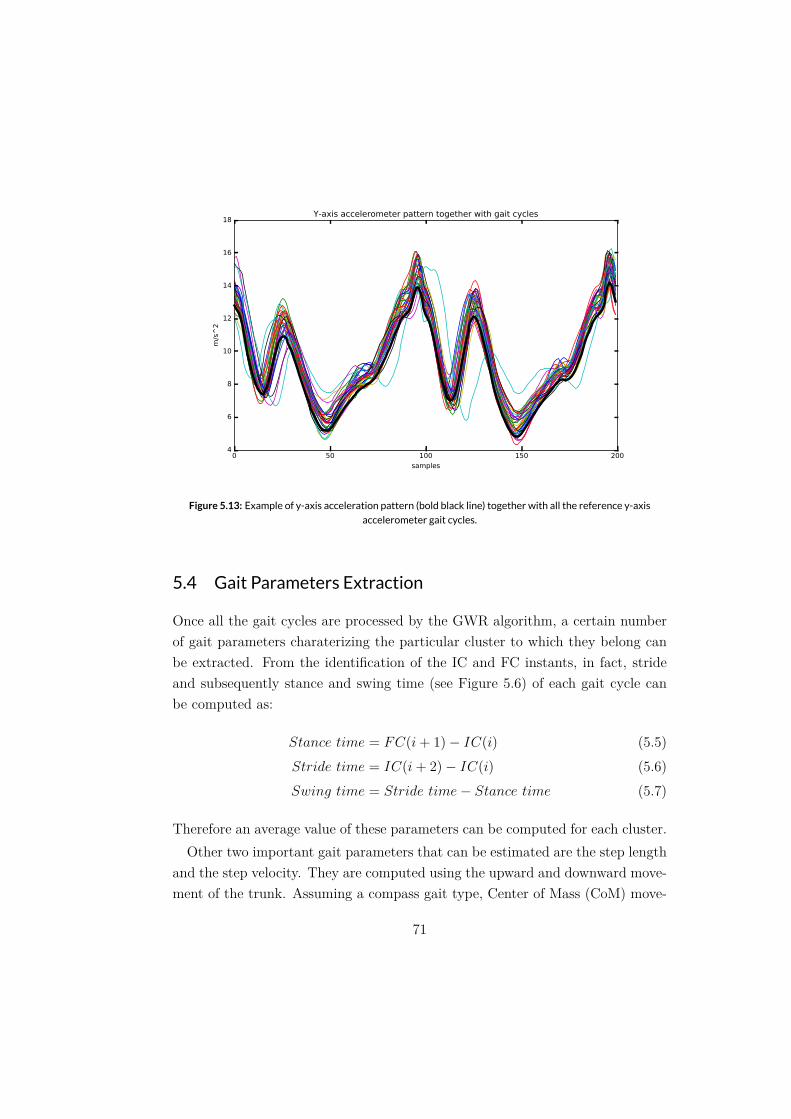
Figure 5.13: Example of y-axis acceleration pattern (bold black line) together with all the reference y-axis
accelerometer gait cycles.
5.4 Gait Parameters Extraction
Stance time = FC(i+ 1)− IC(i)
Stride time = IC(i+ 2)− IC(i)
Swing time = Stride time− Stance time
Step length = 2√2lh− h2.
h l
ay
h
l
Step velocity = Step length/Stride time.
6
6.1 Android Programming
6.1.1 Android Architecture
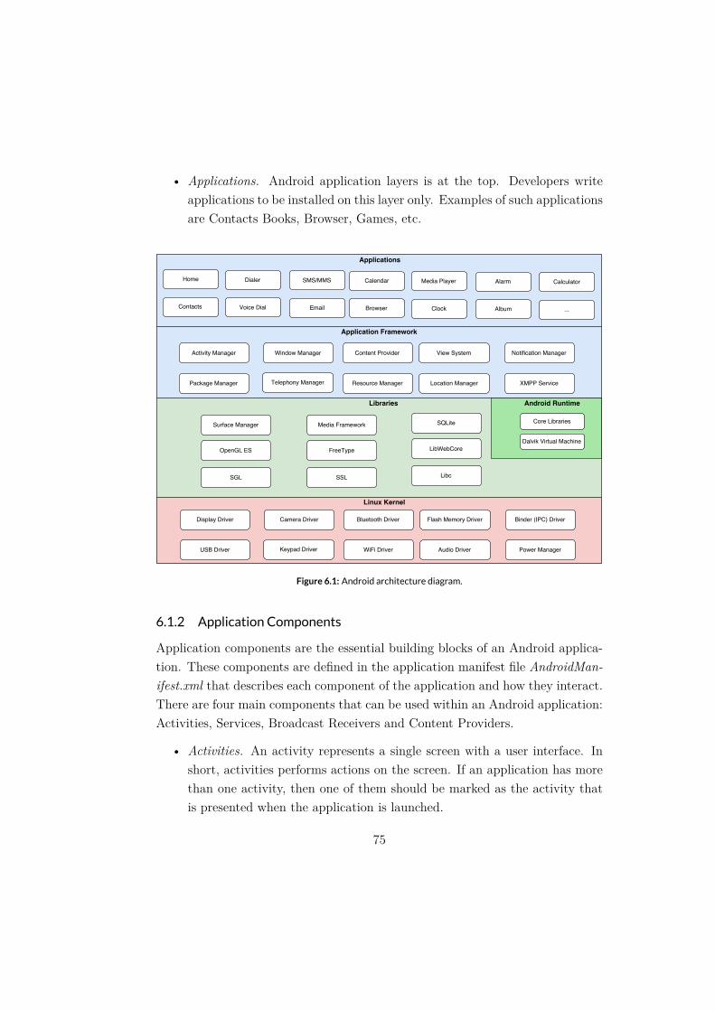
Figure 6.1: Android architecture diagram.
6.1.2 Application Components
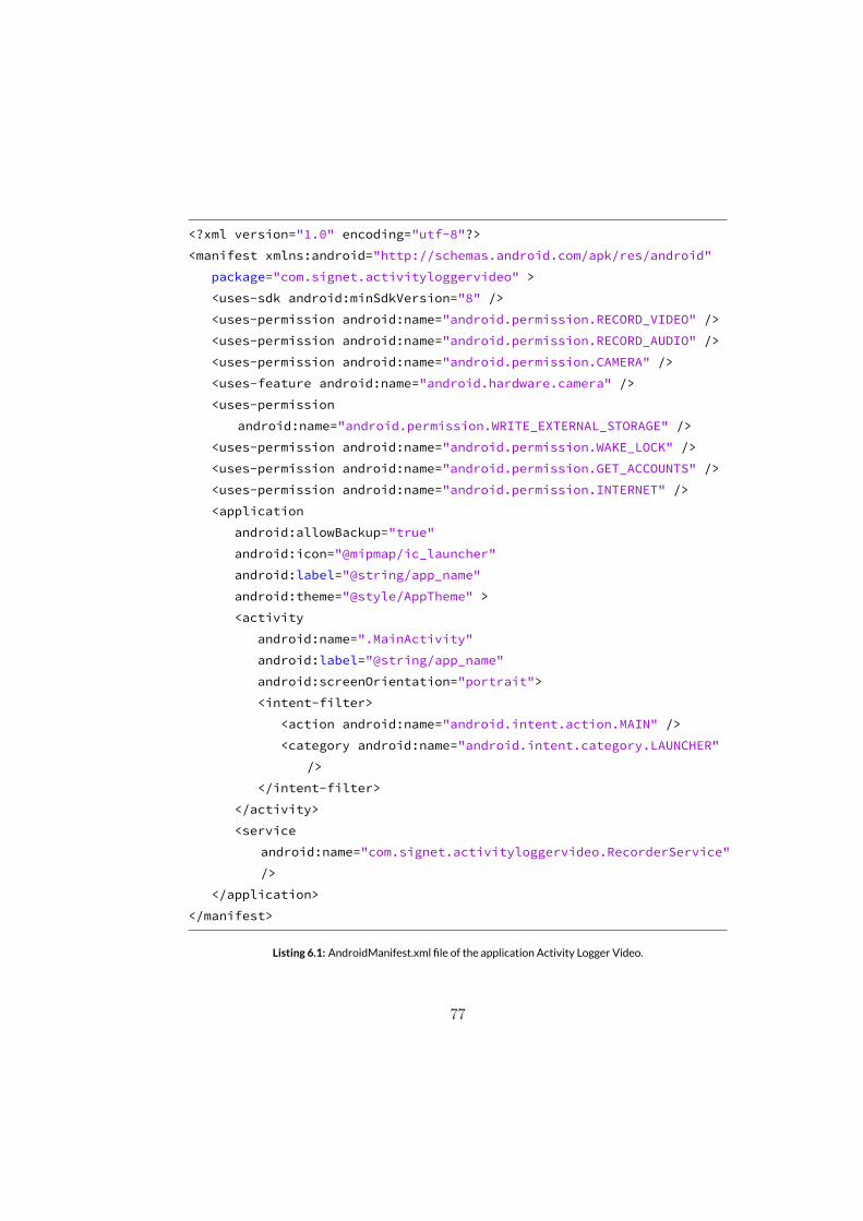
6.2 Activity Logger Video
<?xml version="1.0" encoding="utf-8"?><manifest xmlns:android="http://schemas.android.com/apk/res/android"
package="com.signet.activityloggervideo" ><uses-sdk android:minSdkVersion="8" /><uses-permission android:name="android.permission.RECORD_VIDEO" /><uses-permission android:name="android.permission.RECORD_AUDIO" /><uses-permission android:name="android.permission.CAMERA" /><uses-feature android:name="android.hardware.camera" /><uses-permission
android:name="android.permission.WRITE_EXTERNAL_STORAGE" /><uses-permission android:name="android.permission.WAKE_LOCK" /><uses-permission android:name="android.permission.GET_ACCOUNTS" /><uses-permission android:name="android.permission.INTERNET" /><application
android:allowBackup="true"android:icon="@mipmap/ic_launcher"android:label="@string/app_name"android:theme="@style/AppTheme" ><activity
android:name=".MainActivity"android:label="@string/app_name"android:screenOrientation="portrait"><intent-filter>
<action android:name="android.intent.action.MAIN" /><category android:name="android.intent.category.LAUNCHER"
/></intent-filter>
</activity><service
android:name="com.signet.activityloggervideo.RecorderService"/>
</application></manifest>
Listing 6.1: AndroidManifest.xml file of the application Activity Logger Video.
String server = "*********";String user = "*********";String pass = "*********";String serverRoad = "*********";
Listing 6.2: Strings identifying the connection parameters in the send_file_FTP class.
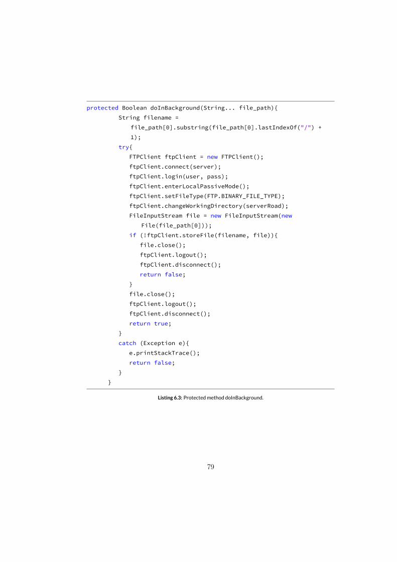
protected Boolean doInBackground(String... file_path){String filename =
file_path[0].substring(file_path[0].lastIndexOf("/") +1);
try{FTPClient ftpClient = new FTPClient();ftpClient.connect(server);ftpClient.login(user, pass);ftpClient.enterLocalPassiveMode();ftpClient.setFileType(FTP.BINARY_FILE_TYPE);ftpClient.changeWorkingDirectory(serverRoad);FileInputStream file = new FileInputStream(new
File(file_path[0]));if (!ftpClient.storeFile(filename, file)){
file.close();ftpClient.logout();ftpClient.disconnect();return false;
}file.close();ftpClient.logout();ftpClient.disconnect();return true;
}catch (Exception e){
e.printStackTrace();return false;
}}
Listing 6.3: Protectedmethod doInBackground.
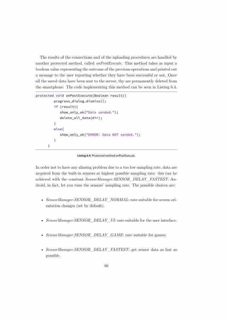
protected void onPostExecute(Boolean result){progress_dialog.dismiss();if (result){
show_only_ok("Data sended.");delete_all_data(dir);
}else{
show_only_ok("ERROR! Data NOT sended.");}
}
Listing 6.4: Protectedmethod onPostExecute.
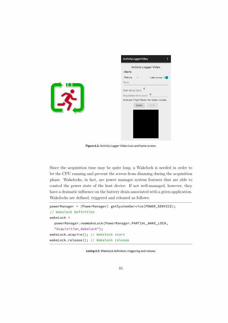
Figure 6.2: Activity Logger Video icon and home screen.
powerManager = (PowerManager) getSystemService(POWER_SERVICE);// Wakelock definitionwakeLock =
powerManager.newWakeLock(PowerManager.PARTIAL_WAKE_LOCK,"Acquisition_Wakelock");
wakeLock.acquire(); // Wakelock startwakeLock.release(); // Wakelock release
Listing 6.5:Wakelock definition, triggering and release.
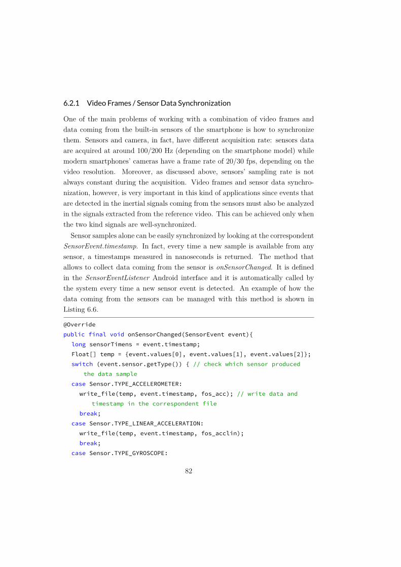
6.2.1 Video Frames / Sensor Data Synchronization
@Overridepublic final void onSensorChanged(SensorEvent event){
long sensorTimens = event.timestamp;Float[] temp = {event.values[0], event.values[1], event.values[2]};switch (event.sensor.getType()) { // check which sensor produced
the data samplecase Sensor.TYPE_ACCELEROMETER:
write_file(temp, event.timestamp, fos_acc); // write data andtimestamp in the correspondent file
break;case Sensor.TYPE_LINEAR_ACCELERATION:
write_file(temp, event.timestamp, fos_acclin);break;
case Sensor.TYPE_GYROSCOPE:
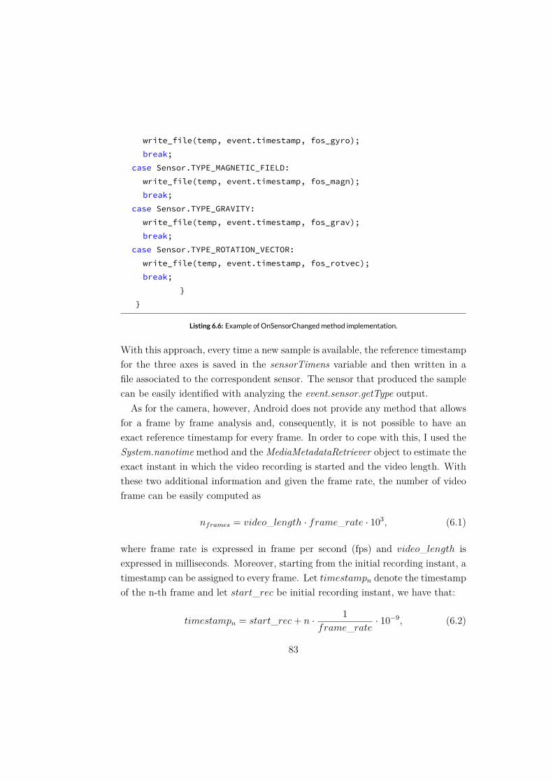
write_file(temp, event.timestamp, fos_gyro);break;
case Sensor.TYPE_MAGNETIC_FIELD:write_file(temp, event.timestamp, fos_magn);break;
case Sensor.TYPE_GRAVITY:write_file(temp, event.timestamp, fos_grav);break;
case Sensor.TYPE_ROTATION_VECTOR:write_file(temp, event.timestamp, fos_rotvec);break;
}}
Listing 6.6: Example of OnSensorChangedmethod implementation.
nframes = video length · frame rate · 103,
video length
timestampnstart rec
timestampn = start rec+ n · 1
frame rate· 10−9,
start rec
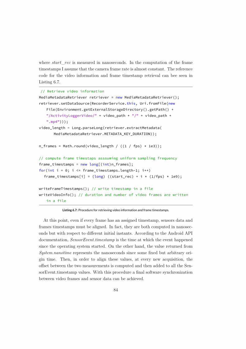
// Retrieve video informationMediaMetadataRetriever retriever = new MediaMetadataRetriever();retriever.setDataSource(RecorderService.this, Uri.fromFile(new
File(Environment.getExternalStorageDirectory().getPath() +"/ActivityLoggerVideo/" + video_path + "/" + video_path +".mp4")));
video_length = Long.parseLong(retriever.extractMetadata(MediaMetadataRetriever.METADATA_KEY_DURATION));
n_frames = Math.round(video_length / ((1 / fps) * 1e3));
// compute frame timestaps asssuming uniform sampling frequencyframe_timestamps = new long[(int)n_frames];for(int i = 0; i <= frame_timestamps.length-1; i++)
frame_timestamps[i] = (long) ((start_rec) + i * (1/fps) * 1e9);
writeFrameTimestamps(); // write timestamp in a filewriteVideoInfo(); // duration and number of video frames are written
in a file
Listing 6.7: Procedure for retrieving video information and frame timestamps.
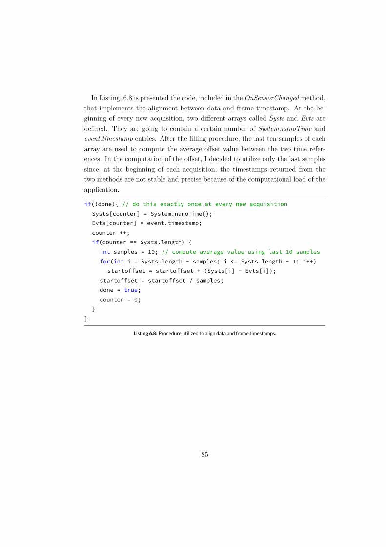
if(!done){ // do this exactly once at every new acquisitionSysts[counter] = System.nanoTime();Evts[counter] = event.timestamp;counter ++;if(counter == Systs.length) {
int samples = 10; // compute average value using last 10 samplesfor(int i = Systs.length - samples; i <= Systs.length - 1; i++)
startoffset = startoffset + (Systs[i] - Evts[i]);startoffset = startoffset / samples;done = true;counter = 0;
}}
Listing 6.8: Procedure utilized to align data and frame timestamps.

7
7.1 GWRClustering
at ∈ [0, 1] at = 1
at = 0
at ht eb en
at ht
at = 0.2
ht = 0.245 eb = 0.3 en = 0.006 ht
Figure 7.1: Firing counter curve and firing counter thresholdht.
amax = 5
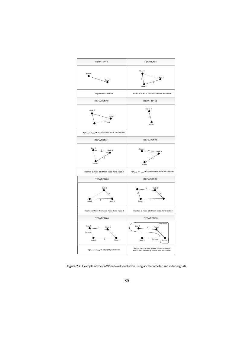
Figure 7.2: Example of the GWRnetwork evolution using accelerometer and video signals.
w2 = (w0 + ξ)/2 w0
ξ
amax
amax
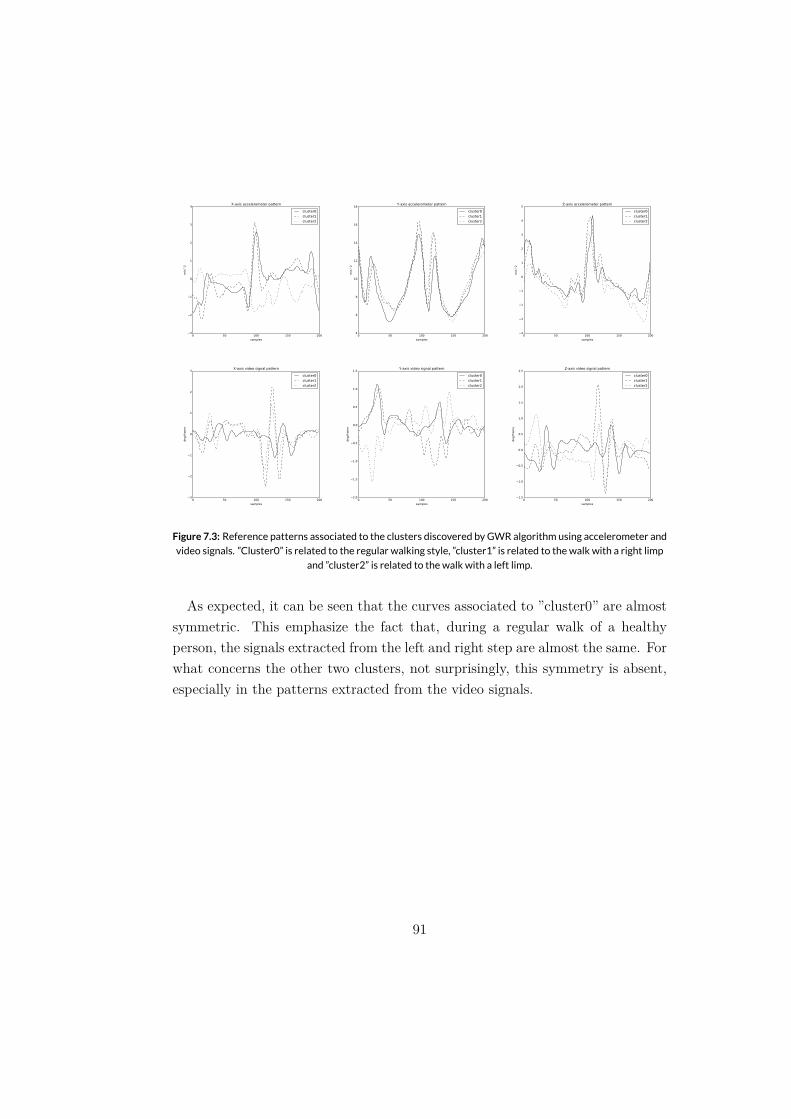
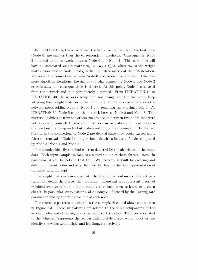
Figure 7.3: Reference patterns associated to the clusters discovered byGWR algorithm using accelerometer and
video signals. ”Cluster0” is related to the regular walking style, ”cluster1” is related to the walk with a right limp
and ”cluster2” is related to the walk with a left limp.
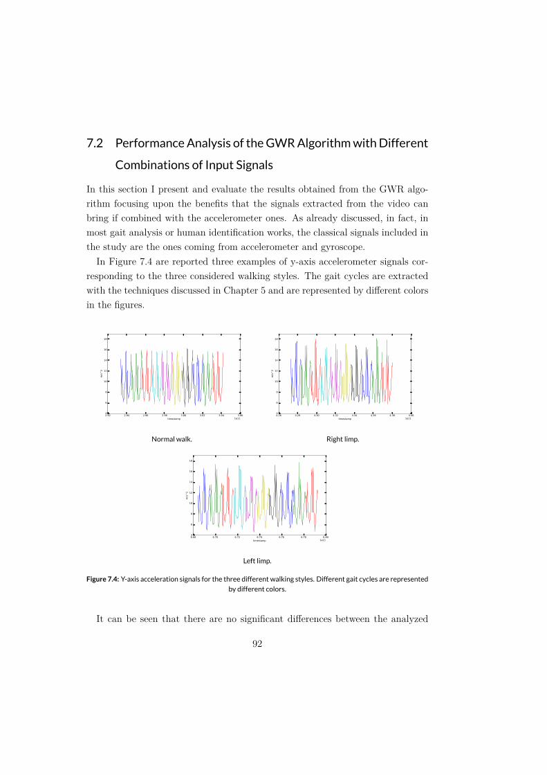
7.2 PerformanceAnalysis of theGWRAlgorithmwithDifferent
Combinations of Input Signals
Normal walk. Right limp.
Left limp.
Figure 7.4: Y-axis acceleration signals for the three different walking styles. Different gait cycles are represented
by different colors.
-30
-20
-10
0
10
20
30
40
featu
re 3
20
feature 2
Clustering results with accelerometer and video signals
0
feature 1
-20
3020100-10-20-30-40
cluster0
cluster1
cluster2
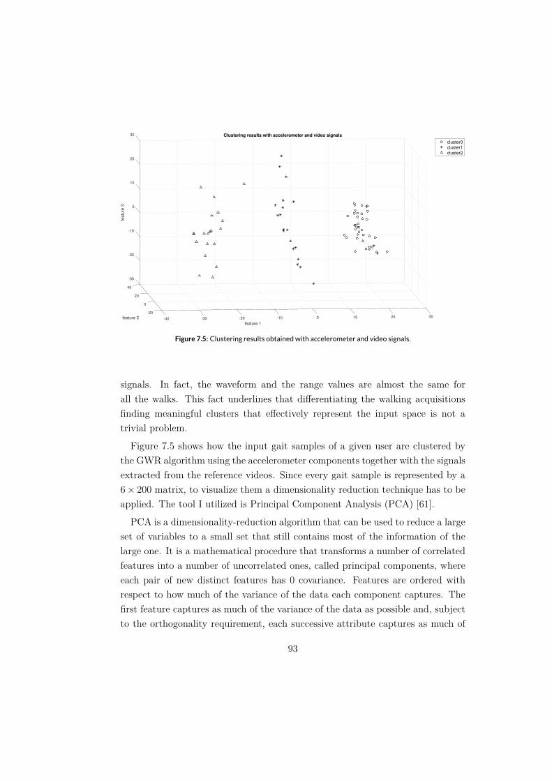
Figure 7.5: Clustering results obtainedwith accelerometer and video signals.
6× 200
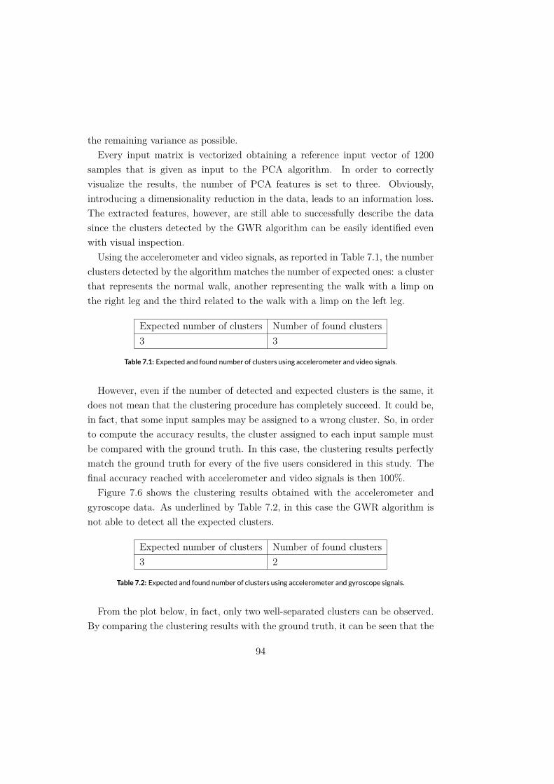
Table 7.1: Expected and found number of clusters using accelerometer and video signals.
100%
Table 7.2: Expected and found number of clusters using accelerometer and gyroscope signals.
-20-10
Clustering results with accelerometer and gyroscope signals
0
feature 2
-20
-15
-10
-5
40 10
0
featu
re 3
5
30
10
15
20
feature 1
10 200 -10 -20 30-30
cluster0
cluster1
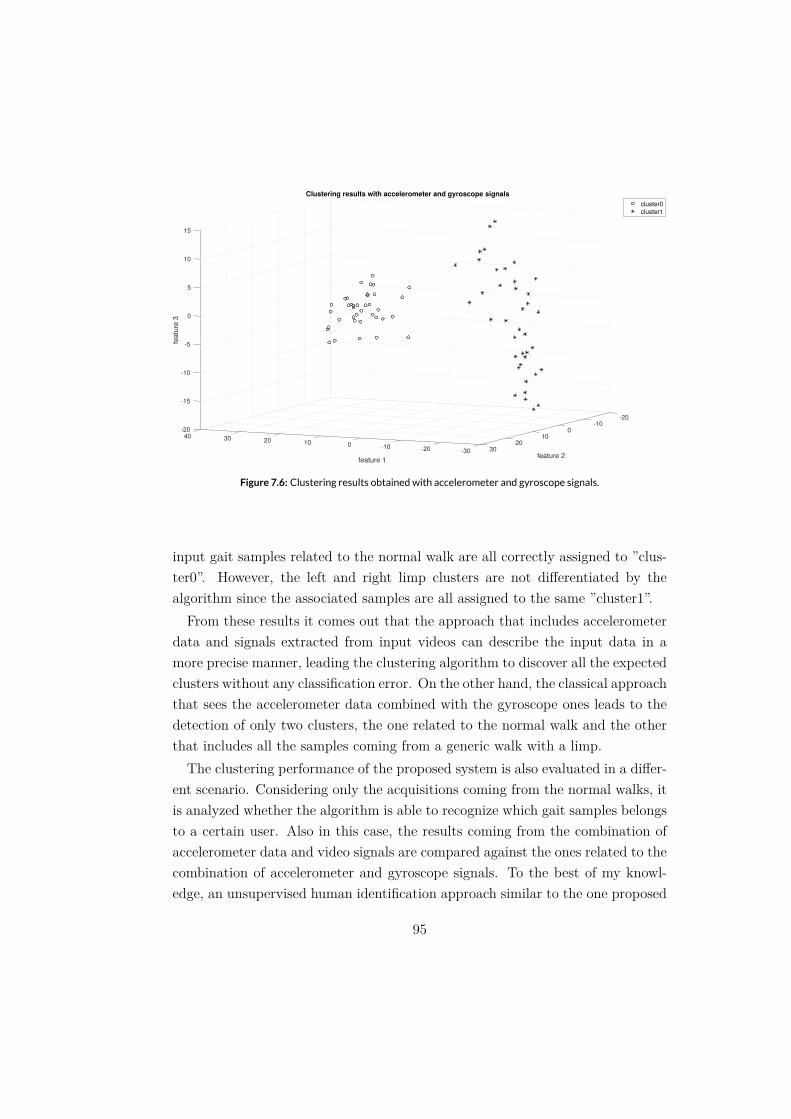
Figure 7.6: Clustering results obtainedwith accelerometer and gyroscope signals.
-40
-20
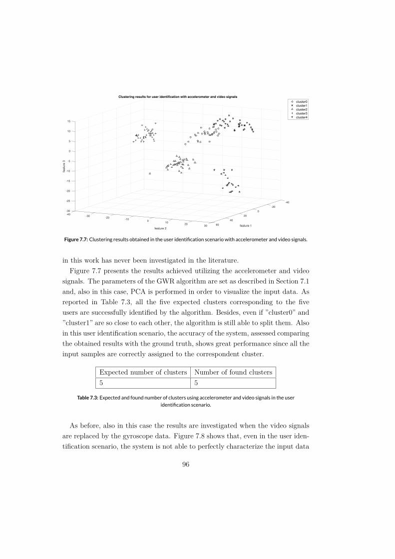
Clustering results for user identification with accelerometer and video signals
0-30
feature 1
-25
-20
-40
-15
-10
20-30
fea
ture
3 -5
0
-20
5
feature 2
10
-10
15
40010
20 6030
cluster0
cluster1
cluster2
cluster3
cluster4
Figure 7.7: Clustering results obtained in the user identification scenario with accelerometer and video signals.
Table 7.3: Expected and found number of clusters using accelerometer and video signals in the user
identification scenario.
-20
-30
-10
-20
-10
0
feature 2
0
featu
re 3
10
10-30
-20-10
feature 1
20 0
20
10
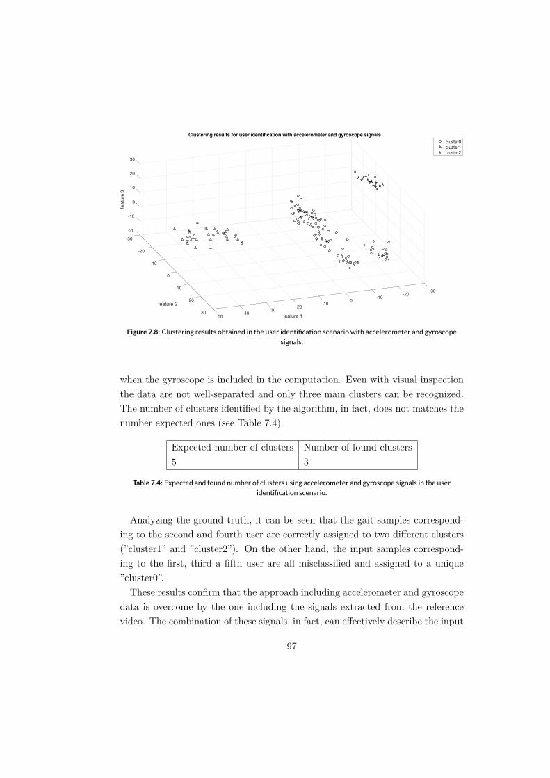
Clustering results for user identification with accelerometer and gyroscope signals
2030
30 4050
30
cluster0
cluster1
cluster2
Figure 7.8: Clustering results obtained in the user identification scenario with accelerometer and gyroscope
signals.
Table 7.4: Expected and found number of clusters using accelerometer and gyroscope signals in the user
identification scenario.
7.3 Gait parameters
± ± ± ± ±± ± ± ± ±± ± ± ± ±
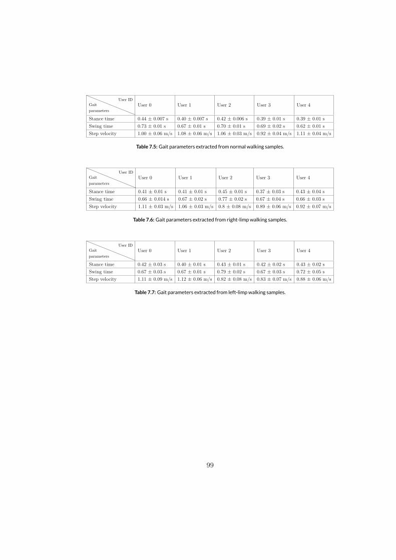
Table 7.5: Gait parameters extracted from normal walking samples.
± ± ± ± ±± ± ± ± ±± ± ± ± ±
Table 7.6: Gait parameters extracted from right-limpwalking samples.
± ± ± ± ±± ± ± ± ±± ± ± ± ±
Table 7.7: Gait parameters extracted from left-limpwalking samples.

8