UNIVERSITÀDEGLISTUDIDIPADOVA …tesi.cab.unipd.it/63312/1/Tesi_LM_P_Dal_Cin_Davide.pdf ·...

UNIVERSITÀ DEGLI STUDI DI PADOVA

Dipartimento di Fisica e Astronomia “GalileoGalilei”

Master Degree in Physics

Final Dissertation

Cosmic Microwave Background anomalies:

models and interpretation

Thesis supervisor: Candidate:

Prof. Nicola Bartolo Davide Dal Cin

Thesis co-supervisor:

Prof. Sabino Matarrese

Academic Year 2018/2019

Contents

Abstract v

1 Introduction 1

2 Λ CDM model 3

3 CMB anomalies 5

4 Non-Gaussian Landscape 94.1 Local Model . . . . . . . . . . . . . . . . . . . . . . . . . . . . 104.2 Beyond Local Model . . . . . . . . . . . . . . . . . . . . . . . . 144.3 Hemispherical power asimmetry . . . . . . . . . . . . . . . . . . 174.4 Response function and OPE expansion . . . . . . . . . . . . . . 22

5 Stochastic Inflation 275.1 Stochastic inflation in a simple two-fields

model . . . . . . . . . . . . . . . . . . . . . . . . . . . . . . . . 30

6 Proposed Model 356.1 Classical evolution . . . . . . . . . . . . . . . . . . . . . . . . . 386.2 Determination of the constants of integration . . . . . . . . . . . 406.3 Construction of the noise terms . . . . . . . . . . . . . . . . . . 43

7 Correlation functions 45

8 Conclusions and futures perspectives 61

Bibliography 63

iii

Abstract

The current standard cosmological model –the so called LambdaCDM model– provides an excellent fit to a variety of cosmological data, in primis the tem-perature anisotropies and polarization of the Cosmic Microwave Background(CMB) radiation. However, as confirmed by the latest Planck satellite data,on the largest angular scales some "anomalies" in the behaviour of the CMBfluctuations have been reported. Despite the fact that their statistical signif-icance remains at the 3-sigma level, they have been independently measuredpreviously also by the WAMP satellite, and at the moment a compelling expla-nation in terms of systematics and or foregrounds does not exist. This mightopen a window into new physics, probably related to the early Universe, sincethe largest scales where these anomalies have been reported are the most sen-sitive to the initial conditions of our universe (e.g. some of these anomalieswould hint to a small deviation from statistical isotropy, which is indeed one ofthe pillars the standard cosmological model is based on). The Thesis aims, firstof all, at providing a review of some of the most important large-scale anoma-lies that have been reported in the CMB data. Then it aims at a detailedstudy of the various cosmological mechanisms that have been proposed so farto explain such features, especially those related to inflationary models (i.e. toan early epoch of accelerated expansion – inflation–the universe went through,which gave rise to the first density perturbations, the seeds for the subsequentformation of all the structures we see in the Universe). An original goal of theThesis work would be in particular to explore possibly new solutions to thesepuzzles, trying to invoke models of inflation characterised by some amount ofprimordial non-Gaussianity. Particular attention would be dedicated in thiscontext to the so called stochastic approach to inflation, where the primordialquantum fluctuations of the fields present during the inflationary epoch arestudied via stochastic equations of motion.

v

Chapter 1

Introduction

The anomalies in the CMB are an interesting puzzle, even today an inflation-ary model that reproduces all the anomalies is not present. In this work wewill focus on the hemispherical power asymmetry. We will study both themodels proposed so far in the literature to explain the anomalies and a possi-ble explicit two-fields model which addresses the problem with the stochasticapproach. A brief summary of the topics covered:

In chapter (2) we present the most important components of the Λ − CDMmodel, and the properties that characterize it. Further references in ModernCosmology (Scott Dodelson) and The Early Universe (Kolb & Turner).

In chapter (3) we analyze the Cosmic Microwave Background (CMB) anoma-lies. These anomalies are in conflict with the standard model of Cosmology.Departures from the model were studied first by Ferreira et al. (1998), Pandoet al. (1998) and in turn, refuted by Banday et al. (2000), Komatsu et al.(2002). Other studies on such departures were made in WMAP CMB mea-surements by Bennett et al. (2003) and recently in the Planck data (PlanckCollaboration XXIII 2014, Planck Collaboration XVI 2016).

In chapter (4) we present the non Gaussian landscape picture and show somemechanisms that can reproduce the large scale hemispherical asymmetry, basedon this model. References on this are Schmidt et al. (2013), Byrnes & Tarrant(2015), Byrnes et al. (2016), Adhikari et al. (2016). These papers are basedon early proposals by Gordon et al (2005), Erickcek et al. (2008), Dvorkin etal. (2008).

In chapter (5) we outline the basic ideas and properties of the stochastic ap-proach to inflation, references on this approach are due to Vilenkin (1983) andStarobinskii (1986). To obtain confidence with the method and the evolutionequations that govern the motion of the fields in the stochastic approach, wediscuss a useful two fields model.

In chapter (6) we introduce the model chosen in this thesis. We then dis-cuss and justify an approximation of which our model is endowed. Thanks to

1

2 CHAPTER 1. INTRODUCTION

this, approximated solutions of the system of Langevin equations are found;also the classical behavior and the noise term are presented.

In chapter (7) the definition of the ζ variable is presented and the two pointfunction is computed at the leading order in the approximation introduced in(6).

In chapter (8) conclusions are shown and future perspectives discussed.

Chapter 2

Λ CDM model

The ΛCDM (Lambda cold dark matter) or Lambda-CDMmodel is a parametriza-tion of the Big Bang cosmological model in which the universe contains threemajor components: first, a cosmological constant denoted by Lambda andassociated with dark energy; second, the postulated cold dark matter (abbre-viated CDM); and third, ordinary matter. It is frequently referred to as thestandard model of Big Bang cosmology because it is the simplest model thatprovides a reasonably good account of the following properties of the cosmos:

1. The existence and structure of the cosmic microwave background (CMB);

2. The large-scale structure in the distribution of galaxies;

3. The abundances of hydrogen (including deuterium), helium, and lithium;

4. The accelerating expansion of the universe observed in the light fromdistant galaxies and supernovae.

The model assumes that general relativity is the correct theory of gravity oncosmological scales. It emerged in the late 1990s as a concordance cosmology,after a period of time when disparate observed properties of the universe ap-peared mutually inconsistent and there was no consensus on the makeup of theenergy density of the universe. The ΛCDM model can be extended by addingcosmological inflation, quintessence and other elements that are current areasof speculation and research in cosmology. As stated previously the letter Λ(lambda) represents the cosmological constant, which is currently associatedwith a vacuum energy or dark energy in empty space that is used to explainthe contemporary accelerating expansion of space against the attractive effectsof gravity. A cosmological constant has negative pressure, p = −ρc2 1, whichcontributes to the stress-energy tensor that, according to the general theory ofrelativity, causes accelerating expansion.The fraction of the total energy density of our ("compatible flat") universethat is dark energy, ΩΛ, is estimated to be 0.669 ± 0.038 based on the 2018Dark Energy Survey results using Type Ia Supernovae or 0.6847±0.0073 based

1We choose as an example an equation of state with w = −1, we underline that to havean expansion the request is w < − 1

3 .

3

4 CHAPTER 2. Λ CDM MODEL

on the 2018 release of Planck satellite data. Another important constituentis dark matter, that is postulated in order to account for gravitational effectsobserved in very large-scale structures (the "flat" rotation curves of galaxies,the gravitational lensing of light by galaxy clusters and enhanced clusteringof galaxies) that cannot be accounted for by the quantity of observed matter.Cold dark matter as currently hypothesized is:

1. Non-baryonic:It consists of matter other than protons and neutrons (and electrons, byconvention, although electrons are not baryons).

2. Cold:It’s kinetic energy is far less than the mass energy at the epoch of freeze-out (thus neutrinos are excluded, being non-baryonic but not cold).

3. Dark:It is not charge under U(1)EM , so it can not interact with photons.

4. Collision-less:The dark matter particles interact with each other and other particlesonly through gravity and possibly the weak force.

5. Stable or long-lived:It has a constant decay time longer than the age of the Universe, so itcan form a relic abundance that can reach us.

Dark matter constitutes about 26.8% of the mass-energy density of the uni-verse. The remaining 4.8% comprises all ordinary matter observed as atoms,chemical elements, gas and plasma, the stuff of which visible planets, starsand galaxies are made. Also, the energy density budget includes a very smallfraction of relic neutrinos and radiation, the so called cosmic microwave back-ground (CMB), discovered in 1965.The CMB offers us a look at the universe when it was only 300,000 years old.The photons in the cosmic microwave background last scattered off electronsat redshift 1100; since then they have traveled freely through space. They aretherefore the most powerful probes of the early universe. In fact up to nowthere has been spent a lot of effort to study in detailed the structure of theCMB. In particular from our first 25 years of surveying the CMB we learnedthat the early universe was very smooth. No anisotropies were detected in theCMB. We are now moving on. We have discovered anisotropies in the CMB,indicating that the early universe was not completely smooth. Recently somestatistical properties (anomalies) in the CMB were found, in tension with thestandard model of cosmology that up to now gave an excellent fit to the CMBanisotropies. Is in fact the main purpose of this work to search for some newsolutions of these interesting puzzles, trying to invoke some models of inflation.Before discussing the models which explain some of the anomalies present inthe CMB, is instructive to explain what the anomalies are.

Chapter 3

CMB anomalies

The CMB is well described by a black-body function with T = 2.725K. An-other observable quantity inherent in the CMB is the variation in temperaturefrom one part of the sky to another. Since the first detection of these temper-ature anisotropies by the COBE satellite, there has been intense activity tomap the sky at increasing level of sensitivity and angular resolution.WMAP and Planck satellites have led to a stunning confirmation of the "Stan-dard model of cosmology". Nevertheless some departures from such modelwere found, first in WMAP and recently in Planck data. Such departures leadto several claims of unexpected statistical properties (anomalies) in the CMBfluctuations. While many of these are significant only at the 2− 3σ level andcould easily be the result of statistical flukes, it is still interesting to specu-late whether they may share a common physical cosmological origin. Firstwe list the six most debated anomalies and then we will investigate whethernon-Gaussianiy alone may be the origin of one of these anomalies. The sixrelevant anomalies are [4]:

1. Local estimates of the angular power spectrum on large scales where theWMAP first-year data indicated an asymmetry of power between twohemispheres on the sky (Eriksen et al. 2004, Hansen et al. 2004). Thishemispherical asymmetry has subsequently been modelled by a dipolarmodulation of an isotropic sky (Eriksen et al. 2007, Hoftuft et al. 2009),and detected at the 2 − 3σ level detection for scales l < 60 in PlanckCollaboration XVI (2016).

2. While the dipolar modulation is detected only on large scales, the spatialdistribution of power on the sky has been shown to be correlated over amuch wider range of multipoles (Hansen et al. 2009, Axelsson et al. 2013,Planck Collaboration XVI 2016). By estimating the power spectrum inlocal patches on the sky for a given multipole range, one can create amap of the corresponding power distribution. Even for an isotropic andGaussian sky, such a map always exhibits a random dipole component.However, it has been shown that the directions of these dipole compo-nents from multipoles between l = 2 to l = 1500 are significantly morealigned in the Planck data than in random Gaussian simulations. Thedirections of these dipoles are close to the direction of the best fit large

5

6 CHAPTER 3. CMB ANOMALIES

scale dipolar modulation of the anomaly 1. But note that anomalies 1and 2 are very different: 1 is present at large scales as an anomalouslylarge dipolar modulation amplitude, whereas anomaly 2 is present atsmaller scales where the amplitude of the observed dipolar modulationis consistent with that expected in the random Gaussian simulations,yet the preferred directions of the dipolar power distribution are alignedbetween multipoles.

3. In Vielva et al. (2004) it was shown that the wavelet coefficients forangular scales of about ' 10 on the sky have an excess kurtosis, whilethe skewness is consistent with zero. The excess kurtosis was shown tooriginate from a cold spot in the southern Galactic hemisphere. How-ever, when masking the spot with a disk of 5 radius, the kurtosis of themap was found to be consistent with Gaussian simulations. The posi-tion of the cold spot on the sky is in the hemisphere where the dipolarmodulation in 1 is positive. Must also be noticed that the cold spot issurrounded by a symmetric hot ring.

4. The Planck andWMAP power spectrum of CMB temperature anisotropyat large scales (l < 30) appears to trend significantly below the val-ues consistent with the best fit cosmological model. In particular, thequadrupole is very low and a dip in the spectrum is observed aroundl ' 21. The low large-scale spectrum could well be a statistical fluctua-tion at these scales where the cosmic variance is large, but the significanceis still at the 2− 3σ level.

5. The quadrupole and octopole appear to be aligned and similarly domi-nated by their respective high-m components (Tegmark et al. 2003).

6. The Cl for the lowest even multipoles has been found to be consistentlylower than for odd multipoles. The significance of this parity anomalyhas been reported to be at the 2 − 3σ level (Planck Collaboration XVI2016).

The correlation between some of these anomalies was studied by Muir et al.(2018) and hence these anomalies were shown to a large degree to be sta-tistically independent. Most of the effort made in the study of the anoma-lies concentrate only on the hemispherical power asymmetry or, at most, inexplaining two anomalies simultaneously. Such models are based on earlierproposals which stated that the properties of the observed CMB sky could bemodelled by the presence of a long-wavelength fluctuation field that modulatesotherwise isotropic and Gaussian fluctuations.In particular, Adhikari et al.[1] have undertaken a systematic and general studyof the power asymmetry expected in the CMB if the primordial perturba-tions are non-Gaussian and exist on scales larger than those we can observe.The analysis focused both on local and non-local models of primordial non-Gaussianity and the method developed is quite general for describing devia-tions from statistical isotropy in a finite subvolume of an otherwise isotropic

7

(but non-Gaussian) large volume. When local non-Gaussianity is invoked,the observed scale dependence of the power asymmetry anomaly can be re-covered by the introduction of two bispectral indices. In Byrnes et al.[8], iscomputed the response of the two-point function to a long-wavelength pertur-bation in models characterized by a local-like bispectrum. However, in all ofthese works only the effects of the second order terms fNL in the primordialnon-Gaussianity have been studied in detail and the main focus was on thelarge-scale power asymmetry. Only recently, in Adhikari et al. [2], it was shownthat large scale power asymmetry may arises in models with local trispectrawith strong scale dependent τNL amplitude. Alternative inflationary modelshave also been proposed to explain other CMB anomalies, such as the lack ofpower at large angular scales and the CMB multipoles alignment [18]. Typi-cally in this case, the models rely on deviations from the usual slow-roll phasein a period immediately before the observable 60 e-folds. In fact, the anomalieson the largest scales could provide hints about the conditions that led to theinflationary dynamics (in the observable window) given that they appear onthe largest scales that will ever be observable.However, the majority of those inflationary models proposed to date to explainthe CMB anomalies have encountered some difficulties. In fact, it seems withour journey knowledge very difficult to construct an inflationary model thatcan reproduce all anomalies and satisfying all today’s bounds. Neverthelessrecently work on this was made by Bartolo et al. [4], even if an inflationarymodel does not appear. Therefore, in this work, we prefer to consider oneanomaly, the hemispherical power asymmetry, and look for toy-models thatcan naturally reproduce it. In particular, inspired by the papers of Adhikari[1], [2] and Byrnes [8], [9], [11] we search for non-Gaussian models, where thenon-Gaussianity is the origin of the above mentioned anomaly in the data.In this perspective it seems natural to review in more detail the fundamentalpapers of Adhikari and Byrnes to better understand the property that unitesthe two articles, the non-Gaussian Landscape.

8 CHAPTER 3. CMB ANOMALIES

Chapter 4

Non-Gaussian Landscape

Inflation is the leading scenario explaining the generation of primordial per-turbations [10]. The observable primordial perturbations probe physics duringthe last αobs ∼ 60 e-foldings of inflation after the horizon exit of the largestobservable modes. Inflation may however have lasted much longer, so that theobservable part of the universe would constitute only a fraction of the entireinflating patch. Long-wavelength perturbations generated before the horizonexit of the largest observable scales average to constants over our observablepatch. Since these contributions are different in different parts of the inflatingregion, variances in the physical properties of patches smaller than the entireinflating region are generated. This leads to a landscape picture where thestatistics of perturbations within a horizon patch depend on the location ofthe patch itself. In a general model we can have αtot > αobs; this implies thatit is not possible to make firm predictions for the observable signatures in ourhorizon patch but one is led to consider probabilities of different signatures. Itturns out that, especially in non-Gaussian models, the differences between theentire inflating patch and a random patch with the size of our observable uni-verse can be significant. Indeed one can calculate the distribution of expecteddeviations from isotropy in our observed sky from any model with isotropicbut non-Gaussian primordial fluctuations. This means that the observationof a violation of the isotropy in our observable universe is "spontaneous", dueto the fact that we concentrate in a subvolume of a larger universe with non-Gaussian fluctuations. But a violation of isotropy, even if apparent, means aprivileged direction. This is a property that characterizes the hemisphericalpower asymmetry as the latter is parameterized as a dipole modulation. Infact the observed C.M.B power asymmetry can be reproduced in models en-dowed of non-Gaussian primordial fluctuations, in particular is no more neededthe enhancing of the amplitude of superhorizon fluctuations. In fact the mostcommon method for introducing a dipolar power modulation is to postulatethe existence of a large-amplitude superhorizon fluctuation in a spectator fieldduring inflation that then alters the power spectrum on smaller scales via local-type non-Gaussianity: the Erickcek-Kamionkowski-Carroll (EKC) mechanism[17]. Now we review the paper of Adhikari where he studied the effects ofnon-Gaussian primordial perturbations on the CMB, starting with the localmodel.

9

10 CHAPTER 4. NON-GAUSSIAN LANDSCAPE

4.1 Local ModelWe assume that, at some early time (after reheating but prior to the release ofthe cosmic microwave background radiation), a large volume of the Universe(Vl) contains adiabatic fluctuations described by isotropic but non-Gaussianstatistics [1]. Since observations are made in a smaller volume, Vs << Vl thatcorresponds in size to our presently observable Hubble volume, we have tounderstand how the statistics of fluctuations in this volume are influenced bythe fluctuations in the large volume. To start we will consider the usual localmodel with constant fNL for simplicity.We can assume that the Bardeen potential Φ is a non-Gaussian field describedby the local model:

Φ(x) = φ(x) + fNL(φ(x)2− < φ(x)2 >

), (4.1)

where φ(x) is a Gaussian random field. When the large volume is only weaklynon-Gaussian, the power spectrum observed in our sky, PΦ,s(k,x), will berelated to the mean power spectrum in the large volume, Pφ(k), by:

PΦ,s(k,x) = Pφ(k)

[1 + 4fNL

∫d3kl(2π)3

φ(kl)eikl·x], (4.2)

where the radial integration for kl is confined to |kl| < πrcmb

, being the CMBspectrum the quantity of interest. The power spectrum Pφ and the amplitudeof non-Gaussianity fNL appearing on the right-hand side of Eq.(4.2) are thosedefined in the large volume.We refer to the paper [1] for the definition of the inhomogeneous power spec-trum; here we only outline the main steps for the derivation of formula (4.2).To obtain this equation, Adhikari starts from the two point function for thevariable Φ. In particular, as stated above, thanks to the weak non Gaussianityonly the linear term in fNL is significant in the power spectrum of the Φ vari-able. When averaging on the entire universe the result is the isotropic powerspectrum Pφ but, if we consider the mean value on a small volume, one of thevariables present in the expectation value is no more stochastic and takes aparticular value. This explains the presence of the field φ(kl) appearing in theintegral. The power spectrum in Eq.(4.2) can depend on the position x withinVs because an individual realization (local value) of the fluctuations φ(kl) canbe nonzero, since the variable is no more stochastic. If we consider the aver-age statistics in the large volume (equivalent to averaging over all regions ofsize Vs), then the term proportional to fNL in Eq.(4.2) averages to zero since< φ(kl) >Vl= 0. In that case we recover the isotropic power spectrum of Vl.To see the effects of the in-homogeneous power spectrum on the CMB we canstart expanding the power spectrum through a multipole expansion:

PΦ,s(k, n) = Pφ(k)

[1 + fNL

∑LM

gLMYLM(n)

], (4.3)

where YLM is a spherical harmonic and n is the direction of observation on thelast scattering surface. To find the expansion coefficients gLM we make use of

4.1. LOCAL MODEL 11

the plane wave expansion:

eikl·x = 4π∑LM

iLjL(klx)Y ∗LM(kl)YLM(n) , (4.4)

where jL is a spherical Bessel function of the first kind and x = xn specifiesthe position of the observed fluctuation: for the CMB x = rcmb is the comovingdistance to the last scattering surface. Eq.(4.2) then implies that:

gLM = 16πiL∫|kl|<π

x

d3kl(2π)3

φ(kl)jL(klx)Y ∗LM(kl) . (4.5)

The quantity gLM has a fixed value in any single volume Vs, but when averagedover all small volumes in Vl, < gLM >Vl= 0 due to the property of the φ(kl)seen before. The expected covariance, on the other hand, is non-zero:

< gLMg∗L1M1

>Vl = 256π2(−1)L1iL+L1

∫|kl|<π

x

d3kl(2π)3

jL(klx)Y ∗LM(kl)×

×∫|k1l|<π

x

d3k1l

(2π)3jL1(k1lx)YL1M1(k1l) < φ(kl)φ∗(k1l) >Vl . (4.6)

We exploit the following relation:

< φ(kl)φ∗(k1l) >Vl= (2π)3δ(kl − k1l)Pφ(kl) ,

and we integrate over kl.Using the orthogonality condition of the sphericalharmonics we get:

< gLMg∗L1M1

>Vl =32

πδLL1δMM1

∫ πx

0

dklk2l j

2L(klx)Pφ(kl)

= 64πδLL1δMM1

∫ πx

0

dklklj2L(klx)Pφ(kl) , (4.7)

where in the last line we have defined the dimensionless power spectrum as:Pφ(k) =

k3Pφ(k)

2π2 .We have again used the subscript Vl to indicate the ensemble average over thevalues of gLM in the full volume Vl. Due to the dependence of the upper limitof integration from the size of the small volume, both the individual valuesof gLM and their variances depend on it. We can now study the monopoleand dipole contributions from non-Gaussian cosmic variance to the modulatedcomponent of the power spectrum in a small volume.

Mono-pole modulation (L=0)

The power-spectrum amplitude shift A0 in the parametrization of Eq.(4.3) is:

PΦ(k) = Pφ(k)[1 + A0] = Pφ(k)

[1 + fNL

g00

2√π

], (4.8)


where A0 can be either positive or negative but has a lower bound A0 ≥ −1.From the previous discussion, it is clear that g00 is Gaussian distributed withzero mean and variance given by:

< g200 >= 64π

∫dklkl

[sin(klx)

klx

]2

Pφ(kl) . (4.9)

Therefore, the distribution of the monopole power modulation amplitude A0

also follows a normal distribution for small values of A01, with zero mean and

standard deviation given by:

σmonofNL=

1

2√π|fNL|2 < g2

00 >12 . (4.10)

The expression for < g200 > is sensitive to the infrared limit of the integral.

That is, all super-Hubble modes can contribute and hence an infrared cut offmust be used. In particular, the observed value of fNL is, in general, shiftedfrom the mean value in the large volume.For a constant fNL, the effect of the monopole modulation is to change thepower-spectrum amplitude on all scales and therefore is not observationallydistinguishable from the “bare” value of the power-spectrum amplitude.The probability distribution for the monopole modulation, as stated above,follows a normal distribution, namely:

pN(A0, σmono) =

1√2πσmono

exp

(− A2

0

2σ2mono

), (4.11)

where the variance has contributions from the Gaussian realization and thenon-Gaussian coupling to the realization of long wavelength modes: σ2

mono =σ2fNL

+σ2G. The term σG is the contribution coming from the Gaussian realiza-

tion. In computing σmonofNLthe necessary infrared cutoff has already been set by

the value of Nextra that can be related to the number of superhorizon e-foldsof inflation. This is, in our simple example, the prediction for the distributionof monopole shift due to non Gaussian modulation. What we see is that thevariance of the distribution of monopole modulations receives a contributionfrom the non-Gaussian coupling to the long wavelenght modes. This contribu-tion is of fundamental importance since the fNL factor is not observable andtherefore it can be increased as to widen the probability distribution and thusmaking the presence of high monopole values shift less anomalous with respectto the Gaussian case. This degree of freedom will be very useful in the case ofthe dipole power asymmetry, as we will see.

Dipole modulation L=1

The dipole modulation of the power spectrum in the parametrization of Eq.(4.3) is given by:

PΦ(k, n) = Pφ(k)

[1 + fNL

M=1∑M=−1

g1MY1M(n)

]. (4.12)

1Follows from the weakly non-Gaussianity assumption in the large volume.

4.1. LOCAL MODEL 13

Since we are interested in the dipole modulation of the observed power spec-trum in the CMB sky, the above equation should be obtained from Eq.(4.2)by absorbing the (unobservable) monopole shift to the observed power spec-trum. On the right-hand side of the previous equation Pφ(k) is the observedisotropic power spectrum and fNL is the observed amplitude of local non-Gausianity within our Hubble volume. This holds also for higher correlationfunctions, for example for the bispectrum we have [1]:

< Φ(k1)Φ(k2)Φ(k3) >= (2π)3δ(~k1 + ~k2 + ~k3)Bobs(k1, k2, k3) , (4.13)

where:

Bobs(k1, k2, k3) = 2fNL(1 + fNLg00)Pφ(k1)Pφ(k2) + sym . (4.14)

Since the observed isotropic power spectrum is P obsΦ = Pφ(1 + fNLg00), insert-

ing this expression in the previous equation one obtains the shift of the fNLfrom the bare to the observed value, namely f obsNL = fNL/(1 + fNLg00) 2.Returning to the monopole modulation, the g1M coefficients are Gaussian dis-tributed with zero mean and variance:

< g1Mg∗1M >= 64π

∫dklkl

[sin(klx)

(klx)2− cos(klx)

klx

]2

Pφ(kl) . (4.15)

If we pick a direction ~di in which to measure the dipole modulation Ai suchthat:

PΦ(k) = Pφ(k)[1 + 2Aicos(θ)] , (4.16)

where cos(θ) = d · n, then the contribution to the dipole from the non-Gaussianity is ANGi = 1

4

√3πfNLg10, which is normally distributed with zero

mean and standard deviation:

σfNL =1

4

√3

π|fNL| < g2

10 >12 . (4.17)

The above discussion about the distribution of the dipole asymmetry Ai as-sumes that we measure Ai in a fixed direction ~d. However, we have no apriori choice of direction ~d in most situations. This is especially true whenconsidering a power asymmetry that is generated by the random realization ofsuperhorizon perturbations as opposed to a single exotic perturbation mode.This means that possible observations of dipole power modulations are nec-essarily reported using the amplitude of dipole modulation in the directionof the maximum modulation. We can obtain this amplitude considering anythree orthonormal directions (d1, d2, d3) on the CMB sky and measuring thecorresponding three dipole modulation amplitudes (A1, A2, A3) along the threeselected directions for each sky. The amplitude of modulation for the CMB

2Abuse of notation fobsNL is the fNL in (4.12).


sky is then given by A =√A2

1 + A22 + A2

3. Clearly then, A follows the χdistribution with three degrees of freedom:

pχ(A, σ) =

√2

π

A2

σ3exp

(− A2

2σ2

), (4.18)

where σ2 = σ2fNL

+ σ2G. What we can do now is to test the analytic calcula-

tions for monopole and dipole power modulations using numerical realizationsof CMB maps. In particular with (4.11) and (4.18) we predict the possiblevalues of dipole and monopole modulations that could be present in the CMB.In particular in this formulas, the presence of σfNL plays the role of widen thedistribution and makes the high value of the dipole modulation less anomalousrespect to the Gaussian case. Clearly the values of σfNL depends on the par-ticular fNL and so equations (4.11) and (4.18). But we can turn over this viewand use the observed asymmetry for parameter estimation of the non-Gaussianamplitude fNL. Combining fNL constraints from bispectrum and power asym-metry measurements we can evaluate the Bayesian evidence for fNL 6= 0. Inour simple examples, the observed CMB power asymmetry only provides weakevidence for non-Gaussianity on large scales [1].

4.2 Beyond Local ModelUp to now we have discussed in detail the effect of local-type non-Gaussianitywith constant fNL that couples superhorizon modes across the CMB sky to theobservable modes. Of course, the anomaly is found to be scale dependent andso this explanation can be considered only an approximation. In particular, toget closer to reality, both the amplitude of the asymmetry and the amplitudeof non-Gaussianity must sharply decrease on smaller scales.A more detailed study is necessary for scale dependent modulations, as theasymmetry we want to reproduce is strongly scale dependent. To addressthe question of how to generate a scale dependent modulations, we will firstdemonstrate that such modulations are a generic feature of non-Gaussian mod-els other than the local model. In fact one can easily extend the inhomoge-neous power spectrum calculation in the presence of local non-Gaussianity toother bispectrum shapes. We can start considering that a Fourier mode of theBardeen potential is given by [1]:

Φ(~k) = φ(~k) +fNL

2

∫d3~q1

(2π)3

∫d3~q2φ(~q1)φ(~q2)N2(~q1, ~q2, ~k)δ(~k− ~q1− ~q2) + . . . ,

where, as before, φ is a Gaussian field. The kernel N2 can be chosen to generateany desired bispectrum and the dots represent higher order terms in powersof φ. Considering only the generic quadratic term, the power spectrum insub-volumes can be computed as in the case of the local bispectrum, and weget:

PΦ,S(k, ~x) = Pφ(k)

[1 + 2fNL

∫d3~kl

(2π)3φ(~kl)N2(~kl,−~k,~k)eı

~kl·~x

].

4.2. BEYOND LOCAL MODEL 15

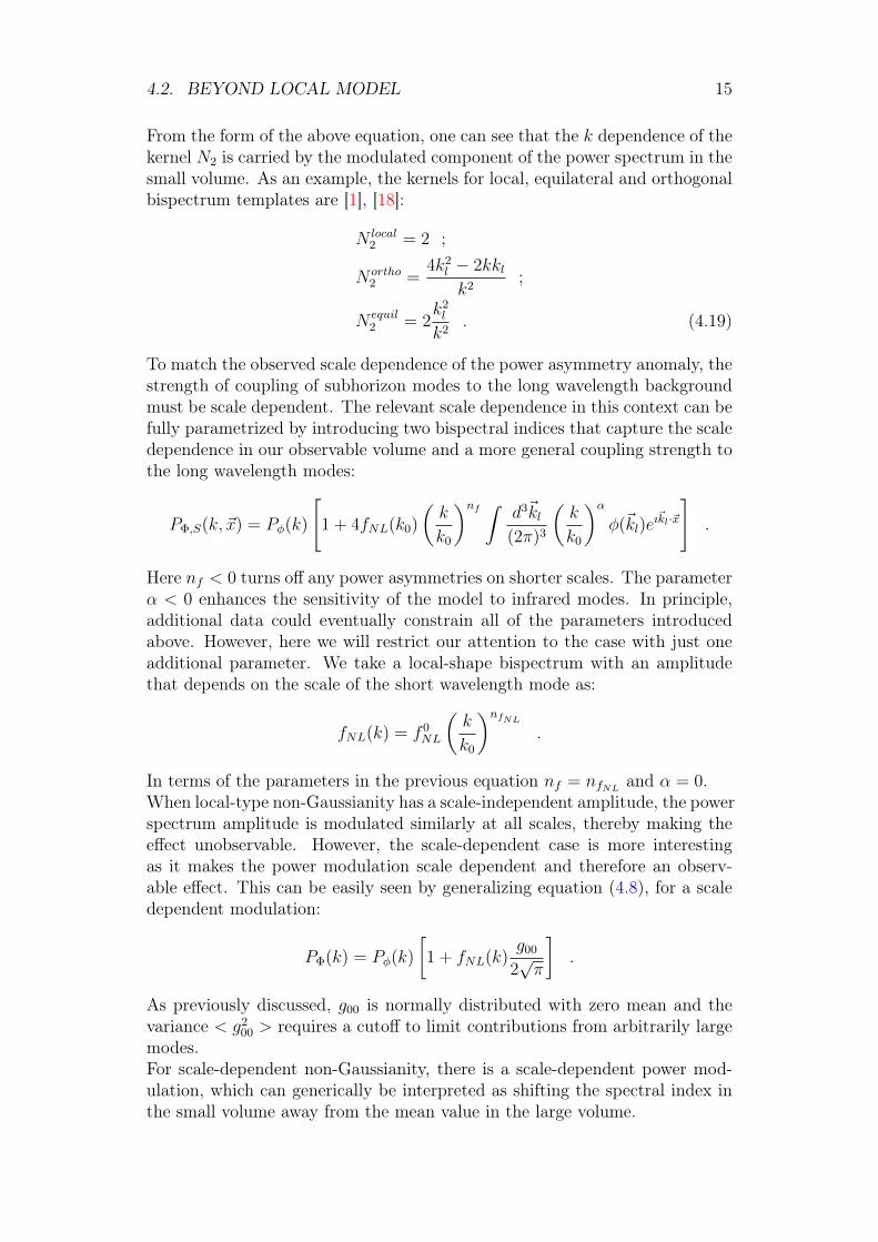
From the form of the above equation, one can see that the k dependence of thekernel N2 is carried by the modulated component of the power spectrum in thesmall volume. As an example, the kernels for local, equilateral and orthogonalbispectrum templates are [1], [18]:

N local2 = 2 ;

N ortho2 =

4k2l − 2kklk2

;

N equil2 = 2

k2l

k2. (4.19)

To match the observed scale dependence of the power asymmetry anomaly, thestrength of coupling of subhorizon modes to the long wavelength backgroundmust be scale dependent. The relevant scale dependence in this context can befully parametrized by introducing two bispectral indices that capture the scaledependence in our observable volume and a more general coupling strength tothe long wavelength modes:

PΦ,S(k, ~x) = Pφ(k)

[1 + 4fNL(k0)

(k

k0

)nf ∫ d3~kl(2π)3

(k

k0

)αφ(~kl)e

ı~kl·~x

].

Here nf < 0 turns off any power asymmetries on shorter scales. The parameterα < 0 enhances the sensitivity of the model to infrared modes. In principle,additional data could eventually constrain all of the parameters introducedabove. However, here we will restrict our attention to the case with just oneadditional parameter. We take a local-shape bispectrum with an amplitudethat depends on the scale of the short wavelength mode as:

fNL(k) = f 0NL

(k

k0

)nfNL.

In terms of the parameters in the previous equation nf = nfNL and α = 0.When local-type non-Gaussianity has a scale-independent amplitude, the powerspectrum amplitude is modulated similarly at all scales, thereby making theeffect unobservable. However, the scale-dependent case is more interestingas it makes the power modulation scale dependent and therefore an observ-able effect. This can be easily seen by generalizing equation (4.8), for a scaledependent modulation:

PΦ(k) = Pφ(k)

[1 + fNL(k)

g00

2√π

].

As previously discussed, g00 is normally distributed with zero mean and thevariance < g2

00 > requires a cutoff to limit contributions from arbitrarily largemodes.For scale-dependent non-Gaussianity, there is a scale-dependent power mod-ulation, which can generically be interpreted as shifting the spectral index inthe small volume away from the mean value in the large volume.


In this paper we have seen how the presence of non Gaussian primordial pertur-bations that exist, with no special features, on scales larger than those we canobserve, modulate the power spectrum observed in sub-volume. We have seendifferent modulations that can be either scale independent or dependent. Inthe case of a scale dependent non-Gaussianity of the localtype this is sufficientto generate a dipole power asymmetry at large scales without invoking exoticsuperhorizon fluctuations. In particular the model considers only the secondorder term fNL as primordial non Gaussianity, neglecting possible higher or-der. The value for fNL chosen to make the observed power asymmetry nolonger anomalous is consistent with the rather weak large-scale constraint, butis well above the scale-independent bound [1].At this point one can wonder what are the effects of possible higher ordermodulations. To address this question we follow Adhikari, who showed thatlarge scale power asymmetry may arise in models with local trispectra withstrong scale dependent τNL amplitude [2]. So in the next section we review indetail his paper.

4.3. HEMISPHERICAL POWER ASIMMETRY 17

4.3 Hemispherical power asymmetry from scaledependent tri-spectrum

We have just seen the general relationship between statistical anisotropies ob-served in a finite volume when the curvature fluctuations on larger scale arecoupled to those on smaller scales [2]. Moreover there has been a lot of effortsto model the observed statistical anisotropies in the CMB. The models canroughly can be categorized into two groups in which:

1. There is an explicit breaking of statistical isotropy , which means a pre-ferred direction in the Universe.

2. The statistical isotropy breaking is spontaneous due to some stochasticmodulating field or primordial non-Gaussianity.

In his work [2], Adhikari, uses a framework where the observed power asym-metry arises spontaneously as the result of looking at a sub-volume of a largerspace whose fluctuations are described by isotropic but non-Gaussian statis-tics. In a non-Gaussian model, the dipolar modulation of the Fourier spacetwo-point function is described by the collapsed limit of the Fourier space four-point function (the trispectrum) of primordial fluctuations.Moreover he studied the effect of a scale-dependent trispectrum in the CMBfluctuations by calculating the induced nonGaussian covariance of modulationestimators. This approach is similar to the previous one, in fact previouslywe have seen the link between the presence in the variance of a non Gaussianmodulation and the resulting less anomaly of a presence of a power modulationin the CMB. Still this approach is more general, since such formalism allowsto simultaneously consider the effect on the modulations expected in the CMBpolarization and forecast the improvement in trispectrum constraints whenadding polarization data. To see that this formalism, namely a modulationfrom a scale-dependent primordial trispectrum, can explain the hemispheri-cal power asymmetry we start from the multipole moments of temperature orpolarization fluctuations, which depend on the primordial potential Φ(~k) asfollows:

axlm = 4π(−ı)l∫

d3~k

(2π)3Φ(~k)gxl (k)Y ∗lm(k) , (4.20)

where gxl (k) is the CMB transfer function with x = T,E describing tempera-ture and E-mode polarization fluctuations respectively.Here we will write down the general expressions for the covariances of modula-tion estimators in the presence of a trispectrum. To see this we start definingthe dipole modulation estimators using l, l + 1 correlations as follows:

∆Xwx0 (l) =

1

(2l + 1)√Cwwl Cxx

l+1

l∑m=−l

aw∗lmaxl+1,m ; (4.21)

∆Xwx1 (l) =

1

(2l + 1)√Cwwl Cxx

l+1

l∑m=−l

aw∗lmaxl+1,m+1 ; (4.22)


where w, x can be either T, E and Cls are the CMB angular power spectrumof the best-fit cosmology. Similar estimators can be defined for higher-ordermodulations, by considering l, l+ 2 correlations: for example, for quadrupolarmodulation. If the primordial fluctuations are Gaussian, the covariance of thedipole modulation estimators is given by:

< ∆Xwx∗M (l)∆Xyz

M ′(l′) >G=

δM,M ′δl,l′

2l + 1

Cwyl Cxz

l+1√Cwwl Cxx

l+1Cyyl′ C

zzl′+1

, (4.23)

where M,M ′ = 0, 1. The two estimators ∆X0(l) and ∆X1(l) contain three de-gree of freedom that determine the amplitude and direction of the dipole mod-ulation. The estimator ∆XM measures a possible dipole modulation present inthe primordial power spectrum in models that generate a CMB power asym-metry by explicitly changing the power spectrum. In this case the means of∆XM are non-zero: < ∆XM(l) >6= 0.The situation is different in models where the primordial fluctuations havesignificant non-Gaussianity. In this case it is possible that global isotropy isrespected, i.e. < ∆XM(l) >= 0, but the expected cosmic variance of CMBdipolar modulation increases. In fact the increment is due to the presence ofthe non Gaussian contribution.We can calculate this contribution to the covariance that depends on a partic-ular configuration of the CMB trispectrum:

< ∆Xwx∗M (l)∆Xyz

M ′(l′) >nG= δM,M ′

∑m,m′ < awlma

x∗l+1,m+Ma

y∗l′m′a

zl′+1,m′+M ′ >c

(2l + 1)(2l′ + 1)√Cwwl Cxx

l+1Cyyl′ C

zzl′+1

,

(4.24)where the subscript c indicates connected part of the trispectrum. To computethe CMB four-point function we follow the method in W. Hu (2001) [5], [6],which constructs the CMB trispectrum from a “reduced trispectrum” that au-tomatically enforces the trispectrum to have rotation, parity and permutationsymmetries. The CMB four-point function can be written using Wigner-3jsymbols, as:

< awl1m1axl2m2a

yl3m3a

zl4m4 > =

∑LM

Pwl1xl2yl3zl4

(L)

(l1 l2 Lm1 m2 −M

)×

×(l3 l4 Lm3 m4 M

)(−1)M + (l2 ↔ l3) + (l2 ↔ l4)

(4.25)

where:

Pwl1xl2yl3zl4

(L) =T wl1xl2yl3zl4(L) + (−1)L+l1+l2T xl2wl1yl3zl4

(L) + (−1)L+l3+l4T wl1xl2zl4yl3(L)+

+ (−1)l1+l2+l3+l4T xl2wl1zl4yl3(L) . (4.26)

The reduced CMB trispectrum T depends on the model of primordial trispec-trum. In this work, we will consider a scale-dependent local τNL trispectrum:


[7]

T (~k1, ~k2, ~k3, ~k4) = τNL

(k2k4

k2p

)nP (k1)P (k3)P (|~k1 − ~k2|) + permutations ,

where the index n describes the scale dependence of the trispectrum ampli-tude of the otherwise local-type trispectrum, and kp is the pivot at which theamplitude is τNL; we take kp = 0.05Mpc−1. Similar to the calculation for theconstant τNL trispectrum, we obtain [6]:

T wl1xl2yl3zl4(L) = τNLhl1l2Lhl3l4L

∫dr1r

21α

wl1

(r1, n)βxl2(r1)

∫dr2r

22α

yl3

(r2, n)×

×βzl4(r2)FL(r1, r2) (4.27)

where:

hl1l2L =

√(2l1 + 1)(2l2 + 1)(2L+ 1)

4π

(l1 l2 L0 0 0

). (4.28)

We define:

αwl (r, n) =2

π

∫dkk2

(k

kp

)ngwl (k)jl(kr) ; (4.29)

βxl (r) = 4π

∫dk

kP (k)gwl (k)jl(kr) ; (4.30)

FL(r1, r2) = 4π

∫dK

KP (K)jL(Kr1)jL(Kr2) , (4.31)

and the jl are spherical Bessel functions. Note that the angular power spectrumcan be written as an integral over the comoving distance r, using the quantitiesαl(r) and βl(r) defined above:

Cwxl =

∫drr2αwl (r, 0)βxl (r) . (4.32)

Adhikari numerically evaluated the reduced trispectrum of equation (4.27) al-lowing him to compute the non-Gaussian covariances, for the dipole modula-tion estimators [2]. The full covariance matrix for dipole modulation estimators(including the fsky scaling for partial sky coverage and the noise power spectra)is given by:

C =< ∆Xwx∗M (l)∆Xyz

M ′(l′) >

=1

(2l + 1)fsky

δM,M ′√Cwwl Cxx

l+1Cyyl′ C

zzl′+1

[δl,l′C

wyl Cxz

l+1+

+1

2l′ + 1

∑m,m′

< awlmax∗l+1,m+Ma

y∗l′m′a

zl′+1,m′+M ′ >c

], (4.33)

where w, x, y, z can be T,E, while M,M ′ = 0, 1 and Cwyl = Cwy

l,cmb + Cwyl,noise.

The noise power spectrum for Planck is approximated using the specifications


for two channels as in S.Galli [21], with fsky = 0.65. For numerical evaluations,Adhikari used camb A. Lewis [22] to obtain the transfer functions gl(k) usingPlanck 2015 best-fit cosmological parameters P.A.R. Ade [23].In the rest of the work [2], Adhikari has numerically evaluated these covari-ances obtaining a fiducial set of scale dependent trispectrum parameters3 thatcan explain the observed hemispherical power asymmetry at large scales andstudied how including polarization and higher-order modulations could im-prove model constraints. Moreover he discussed the non-Gaussian covarianceof angular power spectra generated by a scale-dependent primordial trispec-trum and how it could bias the reconstruction of the spectral index of thepower spectrum. So, by using a scale-dependent local-type trispectrum whichhas a large collapsed-limit signal i.e. in which long-wavelength modes aresignificantly coupled to small scale modes, the following primary results areobtained:

1. Two of the large-scale CMB temperature anomalies — the hemisphericalpower asymmetry and the power deficit at large scales — can be well-modeled by such model;

2. Such a trispectrum has other modulating effects on the temperature andpolarization fluctuations that can be used to improve constraints on thescale-dependent trispectrum parameters;

3. If we require the trispectrum amplitude and parameters be large enoughto explain both the hemispherical power asymmetry and the power deficitat large scales, then we find that the non-Gaussian covariance betweenthe measured angular power spectra of the CMB can be large enough tosignificantly bias the inference of cosmological parameters.

What we have seen so far, is that in both papers of Adhikari [1], [2], the mainidea to explain the hemispherical power asymmetry is to use the non-Gaussianlandscape picture, namely the influence of long-wavelength modes to the ob-served statistic in sub-volumes. In fact in both articles these modes are used tomodulate the variance of the expected dipole modulation making less anoma-lous the presence of a power asymmetry in the CMB data. Nevertheless bothpapers don’t address the issue of an inflationary model that can explain thepower asymmetry, in fact in both articles they assume the form of the Bardeenpotential or directly a particular trispectrum. But if we would find an infla-tionary model that gives us a particular form of the Bardeen potential or aparticular trispectrum we will be able to predict, thanks to the acquired skills,the most probable value of the power modulation expected in a random patchof our universe, with typical size our Hubble volume. This give us a completeand robust recipe to tackle the problem of the hemispherical power asymmetry.So, now what we want to do is try to see if there could be some inflationarymodel that can give us the trispectrum used by Adhikari [2]. The choice ofthe model is not simple, due to both the presence of a plethora of models inliterature, and the fact that is difficult to find a one to one connection between

3Fiducial parameters τNL = 2 · 104 and n = −0.68.


the previous trispectrum and a class of models that can generate it.We will be obliged to choose a particular model, as a general calculation isa hard obstacle; hence is useful to review some papers where an inflationarymodel is used to explain the power asymmetry. In this way we will start learn-ing which models can work and which fail in reproducing the power asymmetry.Fundamental works on this arguments were made by Byrnes [8], [9], [11].


4.4 Response function and OPE expansionIn the letters [8] and [9] Byrnes reports results for a special set of inflation-ary scenarios which can accommodate the hemispherical asymmetry. Byrnesstarts from the work of Aiola et al.[3], who demonstrated that the asymme-try could be approximately fit by a position-dependent power-spectrum at thelast-scattering surface of the form:

Pobs(k) =k3P (k)

2π2(1 + 2A(k)p · n) , (4.34)

where p represents the direction of maximal asymmetry, n is the line-of-sightfrom Earth, and A(k) is an amplitude which Aiola et al. [3] found to scaleroughly like k−0.5. Byrnes tries to see how an inflationary model can produce anasymmetry which replicates this scale dependence. Furthermore in his works[8] and [9], Byrnes, choosing a primordial bispectrum which is compatible withthe modulation A(k), provides an analysis of the CMB temperature bispec-trum generated by this scale- and shape-dependent primordial bispectrum. Todo this, he introduced an explicit model which can be contrived to match allcurrent observations and also serves as an useful example showing the compli-cations which are encountered. To learn how we can generate the asymmetry,we start denoting the field with scale-dependent fluctuations by σ, and takeit to substantially dominate the bispectrum for the observable curvature per-turbation ζ. The ζ two-point function can depend on σ, or alternatively onany combination of σ and other Gaussian fields. The question to be resolvedis how P (k), the power spectrum of curvature perturbations, responds to along-wavelength background of σ modes denoted δσ(~x).We can answer to the previous question thanks to the fact that this responsecan be computed using the operator product expansion ("OPE") [8], and isexpressed in terms of the ensemble averaged two- and three-point functions ofthe inflationary model. We focus on models in which the primary effect is dueto the amplitude of the long-wavelength background rather than its gradients.Since the perturbation is small it is possible to write:

P (k, ~x) = P (k) (1 + δσ(~x)ρσ(k) + . . . ) . (4.35)

We call ρσ(k) the "response function". The OPE gives [8] :

ρσ(k) ' 1

P (k)

[Σ−1(kL)

]σλBλ(k, k, kL) if k >> kL , (4.36)

where a sum over λ is implied, and Σαβ and Bβ are spectral functions forcertain mixed two- and three point correlators of ζ with the light fields of theinflationary model, which we collectively denote δφα4:

< δφα(~k1)δφβ(~k2) > = (2π)3δ(~k1 + ~k2)Σαβ ;

< δφα(~k1ζ(~k2)ζ(~k3) > = (2π)3δ(~k1 + ~k2 + ~k3)Bα .

4In our framework the sum in (4.36) includes only the σ fields.

4.4. RESPONSE FUNCTION AND OPE EXPANSION 23

In the special case of a slow-roll model in which a single field generates allperturbations, it can be shown that the right-hand side of (4.36) is related tothe reduced bispectrum:

ρσ(k) =12

5fNL(k, k, kL) k >> kL ,

where fNL is defined by:

6

5fNL(k1, k2, k3) =

B(k1, k2, k3)

P (k1)P (k2) + 2cyclic perms.

To proceed further, in (4.36) appear long wavelength background modes thatwe model in this way [9]:

δσ(~x) ≈ EP12σ (kL) cos

(~kL · ~x+ θ

),

where E labels the ‘exceptionality’ of the amplitude, with E = 1 being typicaland E >> 1 being substantially larger than typical. We assume the wavenum-ber kL to be fixed. The phase θ will vary between realizations, and the Earthis located at ~x = 0.The last-scattering surface is at comoving radius xls; evaluating (4.36) on thissurface at physical location ~x = xlsn and assuming α = xlskL

2π< 1 so that the

wavelength associated with kL is somewhat larger than xls, we get:

P (k, ~x) = P (k)

(1− C(k) + 2A(k)

~x · kLxls

+ . . .

). (4.37)

To obtain the last formula, we expand the argument of the back-ground modes,since by assumptions the argument is less than 1.The quantities A(k) and C(k) are determined in terms of the response ρσ andlong-wavelength back-ground by:

A(k) = παEP12σ (kL)ρσ(k) sin θ ;

C(k) = −A(k)cos θ

πα sin θ.

Both A and C share the same scale-dependence, so it is possible to use C(k) toexplain the lack of power on large scales. If so, the model could simultaneouslyexplain two anomalies—although this would entail a stringent constraint onα in order that C(k) does not depress the power spectrum too strongly atsmall l. After having presented the general formulas for the determinationof the response function and, thanks to this, the prediction of the particularscale dependence of the modulation A(k) it’s time now to construct explicitlysome inflationary models that, due to the fact that have a large and negativeη-parameter, can generate a scale dependent modulation that match the scaledependence found by Aiola et al. Starting with the single field model (we havethat when one field dominates the two- and three-point functions of ζ) thebispectrum is equal in squeezed and equilateral configurations [24]. Therefore:

ρσ =12

5fNL(k, k, kL) =

12

5fNL(k, k, k) ,


and since the scale dependence of the asymmetry is determined by the scaledependence of the response function we have in this case that the asymmetryscales in the same way as the equilateral configuration fNL(k, k, k). If thescaling is not too large it can be computed using [7]:

d ln |fNL|d ln k

=5

6fNL

√r

8

M3PV′′′

3H2,

where r < 0.1 is the tensor-to-scalar ratio. To achieve strong scaling we re-quire m3

PV′′′

3H2 >> 1. But within a few e-foldings this will typically generate anunacceptably large second slow-roll parameter ησ, defined by:

ησ =M2

PV′′

3H2.

Therefore it will spoil the observed near scale-invariance of the power spec-trum. As a specific example, a self-interacting curvaton model was studiedin [11]. This gave rise to many difficulties, including logarithmic running offNL(k, k, k) with k, which is not an acceptable fit to the scale dependence ofA(k). Even worse, because the scale dependence of fNL is large only when fNLis suppressed below its natural value, both the trispectrum amplitude gNL andthe quadrupolar modulation of the power spectrum were unacceptable. So inconclusion, the usual models of inflation with a single fields are not good toreproduce the hemispherical asymmetry, at least with this approach, due tothe many difficulties cited above. We must therefore think of other possiblescenarios in which the asymmetry can be reproduced. The immediate exten-sion is to study multi-field models.In multiple-source scenarios there is more flexibility. If different fields con-tribute to the power spectrum and bispectrum it need not happen that a largeησ necessarily spoils scale-invariance. In these scenarios ρσ no longer scaleslike the reduced bispectrum, but rather like its square-root. Therefore:

d lnA

d ln k≈ 1

2

d ln |fNL(k, k, k)|d ln k

≈d ln

(PσP

)d ln k

≈ 2ησ − (ns − 1) , (4.38)

where P is the dimensionless power spectrum, ns − 1 ' −0.03 is the observedscalar spectral index and ησ was defined previously. If we can achieve a con-stant ησ ≈ −0.25 while observable scales are leaving the horizon, then it ispossible to produce an acceptable power-law for A(k), further references [8],[29]. A simple potential with large constant ησ is:

W (φ, σ) = V (φ)

(1− 1

2

m2σσ

2

M4P

).

The inflaton φ is taken to dominate the energy density and therefore drivesthe inflationary phase. Initially σ lies near the hilltop at σ = 0, so its kineticenergy is subdominant and ε ≈ M2

PV2φ /V

2; here ε is the conventional slow-roll parameter. As inflation proceeds σ will roll down the hill satisfying thefollowing equation:

dσ(N)

dN= − Wσ

3H2=

1

3H2V (φ)

σm2σ

M4P

.

4.4. RESPONSE FUNCTION AND OPE EXPANSION 25

On the right hand side, a part for the σ field, we recognize the ησ parameter.The integration of the above equation yields:

σ(N) = σ∗e−ησN ,

where ‘*’ denotes evaluation at the initial time and N measures the number ofsubsequent e-folds. To keep the σ energy density subdominant we must pre-vent it rolling to large field values, which implies that σ∗ must be chosen to bevery close to the hilltop. But the initial condition must also lie outside the dif-fusion dominated regime, meaning the classical rolling should be substantiallylarger than quantum fluctuations in σ. This requires | dσ

dN| >> H∗

2π. In combina-

tion with the requirement that σ remains subdominant in the observed powerspectrum, we find that σ∗ should be chosen so that |σ∗| >

√ε∗PMP/|ησ|.

For typical values of ε = 10−2 and ησ = −0.25 this requires |σ(60)| > 100MP

which is much too large. The problem can be ameliorated by reducing ε∗,but then σ contributes significantly to ε during the inflationary period. Thisreduces the bispectrum amplitude to a tiny value, or causes σ to contaminatethe power spectrum and spoil its scale invariance [8]. To avoid these problems,we consider a potential in which the effective mass of the σ field makes a rapidtransition. An example is:

W = W0

(1 +

ηφ2

φ2

M2P

)(1 +

ησ(N)

2

σ2

M2P

),

where ησ(N) is chosen to be -0.25 while observable scales exit the horizon, laterrunning rapidly to settle near -0.08. We take the transition to occur roughly16 e-folds after the largest observable scales exited the horizon [8]. The field φwill dominate the Gaussian part of ζ and its mass should be chosen to matchthe observed spectral index.The most urgent question is whether the bispectrum amplitude is compati-ble with present constraints for f localNL ,f equiNL , which are weighted averages overthe bispectrum amplitude on groups of related configurations. At present, thestrongest constraints apply to f localNL which averages over modestly squeezedconfigurations. To determine the response of these estimators Byrnes con-structs a Fisher estimate [8]. He numerically computes ∼ 5× 106 bispectrumconfigurations for the above potential covering the range from l ∼ 1 to l ∼ 7000and uses these to predict the observed angular temperature bispectrum. For achoice of parameter values which generate the correct amplitude and scaling ofA(k), he finds that a Planck-like experiment would measure order-unity values,

f localNL = 0.25 ; f equiNL = 0.6 ; f orthoNL = −1.0 .

These estimates are one to two orders of magnitude smaller than possible es-timates based on the EKC mechanism [17] and are easily compatible withpresent-day constraints. We presented this works because is a viable scenariofor which seek an inflationary explanation of the asymmetry. In fact in thispaper much less tension with observation than would be expected on the ba-sis of EKC mechanism is involved, also the difficulty that one can have in


constructing a model in agreement with the stringent bound from Planck arecaught. In fact, to build a successful model we have been forced to make anumber of arbitrary choices, including the initial and final values of the σ mass,and the location and rapidity of the transition. Anyway the line of the thesisis to use the stochastic approach to inflation and an implementation of the ηprocedure is not simple in this framework, so we do not pursue in the followingthis scenario. From this paper we learn that a single field model of inflation isnot capable to reproduce the correct power asymmetry, so we are forced to usemulti-field scenario. In particular using multi-field scenario we evade anothervery important problem. In fact in the adiabatic single field models it is wellknown that the long-wavelength contributions amount to simply shifting thelocal time coordinate. The situation is different if more than one light dy-namical scalar is present during inflation and in this case the long-wavelengthmodes are no more gauge modes and the previous problem is not present.So the next step is to study the properties of a multi-fields system, the simpleone consist in two fields, in stochastic inflation. In the next chapter we explainthe main properties of the stochastic approach to inflation and present an ar-ticle with whom we try our-self with a two fields model in this scenario [13].

Chapter 5

Stochastic Inflation

The simpler models of inflation are implemented through the use of a scalarfield whose dynamics is governed by a classical Klein-Gordon equation [20].This field is moving on a expanding back-ground field metric that we choosein this case to be a FRLW metric with a De Sitter expansion.Not only the classical evolution is important but also the quantum nature ofthe scalar field leads to very interesting physics and the stochastic approachis the natural framework to study it. The approach consists in splitting thescalar field in momentum space into long and short wavelength modes.Starting from the Heisenberg operator equation of motion for the scalar field,the evolution of the long wavelength part satisfies a classical, but stochastic,equation of motion. The quantum effects, in the form of short wavelengthmodes, build up a noise term, as we will explain below. The field satisfies:

∇µ∇µφ+∂V

∂φ= 0 .

The scalar field may be written φ = φlong + φshort, or more explicitly:

φ = φlong(~x, t)+1

(2π)32

∫d3kθ(k−εaH)

(akφk(t)e

−ı~k·~x + a†kφ∗k(t)e

ı~k·~x), (5.1)

where φlong(~x, t) contains only modes such that k << aH; a†k, ak are the usualcreation and annihilation operators, ε is a constant much smaller than 1, andθ stands for the step function.Usually inflation takes place in regions where the scalar field potential is notvery steep and thus the short wavelength part satisfies the mass less equation:

∇µ∇µφshort = 0 .

Thus the short wavelength modes can be taken as:

φk =H√2k

(1

aH+ı

k

)exp

(ık

aH

).

From this, Starobinskii derives the equation of motion for the long wavelength"coarse-grained" part which, in the slow-rolling approximation, reads:

φlong(~x, t) = − 1

3H

∂V

∂φlong+ f(~x, t) , (5.2)

27

28 CHAPTER 5. STOCHASTIC INFLATION

where the spatial gradient of φlong has been neglected since it is sub-dominatfor modes k << aH and hence the evolution of the coarse-grained field can befollowed in each domain independently [14], [15] where:

f(~x, t) =1

(2π)32

∫d3kδ(k − ks)ks

(akφk(t)e


ı~k·~x)

, (5.3)

where ks = εaH stands for the inverse of the coarse-grained domain radius.According to this picture the universe is described by the value of the field indifferent coarse-grained domains of comoving size k−1

s ' (εa1H1)−1.With the inflationary expansion, an initial domain gets divided into sub do-mains, after one Hubble time-step. The magnitude of the coarse-grained field φin these smaller domains is determined by both the classical and the noise partsappearing in the right-hand side of equation (5.2). The classical force "pushes"the field down the potential in all the subdomains, whereas the stochastic forceacts with different strengths and arbitrary direction in different subdomains.This process repeats itself in all subsequent Hubble time-steps.The results of this process is that in the new subdomains the field takes ondifferent values: in those where the classical "drag" overwhelms the stochas-tic "push" the field goes down the potential and inflation will eventually end,yielding a domain like our present universe.However, in those domains where the opposite happens there will be regionswhere the stochastic force is greater than the classical one. In this case we canobtain the so called Linde’s eternal inflation picture, for more information [27].

A very crucial step in order to be able to obtain the correlation function in thestochastic approach, consists in calculate the auto-correlation function for thenoise term [12]. The auto-correlation is:

< f(~x, t)f(~y, t′) >=1

(2π)3

∫d3k

∫d3pδ(p− ks(t′))ks(t′)δ(k − ks(t))×

× ks(t) <(akφk(t)e


ı~k·~x) (apφp(t

′)e−ı~p·~y + a†pφ∗p(t′)eı~p·~y

)> ,

(5.4)

the only term that survive is ak, a†p, using the commutation relation for theannihilation operators this term gives a delta Dirac term δ(~k− ~p). Integratingin ~p we get:

< f(~x, t)f(~y, t′) >=1

(2π)3

∫d3kδ(k − ks(t′))ks(t′)δ(k − ks(t))ks(t)×

×φk(t)φ∗k(t′)eı~k·(~x−~y) , (5.5)

applying the Dirac delta on itself we get δ(ks(t) − ks(t′)). This term can betreated using the property of the Dirac delta and we get δ(t−t′)

εH2a. This implies,

thanks to the delta, the fact that t = t′. Finally we obtain:

< f(~x, t)f(~y, t′) >=1

(2π)3

δ(t− t′)εH2a

(εHa)2

∫d3kδ(k − ks(t))|φk(t)|2eı

~k·(~x−~y) .

(5.6)

29

We used the form of the short-wave length to compute the modulus square.Finally we obtain 1:

< f(~x, t)f(~y, t′) >=H3

4π2j0(ks(t)|~x− ~y|)δ(t− t′) , (5.7)

this is the form of the correlation in the noise for spatially separated points.To be noticed the white noise property in time. The previous relations arequite general, they hold for a general scalar field, minimally coupled to grav-ity, undergoing a slow rollover transition towards a state of lower energy. Thechoice for the scale factor is not crucial for the results. More general acceler-ated expansion laws can be considered; the previous equations will continueto hold provided that we include some numerical coefficients characteristic ofthe considered expansion [16].If we are interested on one particular domain, say with comoving coordinate ~x,then only the delta term remains and at this point one could attempt to studythe probability distribution P (φ, t) for the coarse-grained field φ by means ofthe Fokker-Planck equation. To be complete, due to the time dependence ofthe Hubble parameter, it has been proposed that a more fundamental timevariable, in the Langevin equation, is given by α ∝ ln(a) =

∫dtH(t) [25].

After having introduced the main properties of the stochastic approach to in-flation, namely the division of the field in short and long components, and theevolution of the latter through a stochastic equation of motion of the Langevintype where the noise term is made through the short part of the field. Clearlyup to now, all arguments were made strictly apply to a single field model.When more than one fields are present, we have a system of Langevin equa-tions that are coupled together, rather that two separated equations.As we saw previously, a model of at least two fields is necessary if we wantto reproduce the power asymmetry. So is natural, to move the first steps alsowith the stochastic approach, to review the paper of Matarrese [13], where hestudied a two fields model of inflation in the stochastic approach. Even if inthis paper, the Fokker-Planck equation is solved for a particular model thatwe will see, and Matarrese did not concentrate on the Langevin equation, wereviewed this paper because from this we can capture the difficulty in findinga general solution, and the potential used in this work is very similar to our,and we will understand why this happens.As stated above in Matarrese’s article they concentrate on the Fokker-Planckequation; in our work we will rather concentrate on spatial correlations whichcould be derived from the Langevin-type equation. For completeness one canstudy correlations between different coarse-grained domains using the func-tional form of the Fokker-Planck equation, even if this road is very complexand not very useful.

1We can neglect the ε term present in the final formula, since ε is small by assumption.


5.1 Stochastic inflation in a simple two-fieldsmodel

Inflationary models with more than one scalar fields have been studied withdifferent aims in recent years. In the work [13] the model chosen consistsin a two fields model where one is a free massless field and the inflaton hasan exponential potential, therefore leading to power-law inflation. In spite ofits simplicity, the model displays a number of interesting features, such as themultiplicative effects produced by the inflaton fluctuations on the motion of themassless field, which is expected to occur also in more complicated multiple-field models. Moreover the main statistical properties of the distribution at thedifferent scales of interest are studied. The joint probability for the two fieldsis always found to be non-Gaussian; however, in order that the non-Gaussianfeatures are quantitatively relevant it is necessary that the system starts itsstochastic evolution from a state with an energy density comparable to thePlanck one.To see this interesting property of the model we can proceed as follow: forthe multiplicative effects we have to derive the equations which govern thedynamics of a two scalar-fields system during inflation within the stochasticapproach, specializing our analysis to the axion (massless field) dynamics ina power-law inflation. Then, for the non-Gaussian property of the model,we have to solve the Fokker-Planck equation which governs the evolution ofthe joint probability distribution for our two-field system. Starting from themultiplicative features, as we have seen previously for the evolution of a scalarfield, either the inflaton or any other scalar field in the theory, is described by aLangevin-type equation for a coarse-grained variable. This is usually written interms of the proper time t, but as previously mentioned a better time variableto use is given by α = ln(a/a0) [25]. In terms of the number of e-folding andconsidering the stochastic evolution inside a single coarse grained domain, wehave the system:

dφ

dα= −∂φV

3H2+H

2πηφ(α) ;

dχ

dα= −∂χV

3H2+H

2πηχ(α) ; (5.8)

where H2 = (8π/3m2P )V (φ, χ) with mP the Planck mass; ηφ and ηχ are

Gaussian noises with zero mean and correlation functions < ηφ(α)ηφ(α′) >=δ(α− α′) equal for χ, as previously seen for a single coarse domain.Moreover the two noise terms are assumed to be an-correlated. The twoLangevin equations are said to be of multiplicative type since the coefficientsof the noise terms depend on the random variable itself. The previous systemcan be rewitten in the following way:

∂φ

∂τ= −fφ(φ, χ) + gφ(φ, χ)ηφ(τ) ;

∂χ

∂τ= −fχ(φ, χ) + gχ(φ, χ)ηχ(τ) ; (5.9)

5.1. STOCHASTIC INFLATION IN A SIMPLE TWO-FIELDS MODEL 31

where τ = t, α and the f terms denote the classical force and the g termsthe amplitude of the stochastic noise. The 4 terms are given in the previousequation for the case τ = α and change in the case t = τ . From them we canderive the associated Fokker-Planck equation for the joint probability Pφχ. Inthe so called Stratonovich approach this is given by:

∂Pφχ∂τ

=∂

∂φ

(fφPφχ +

gφ2

∂

∂φ(gφPφχ)

)+

∂

∂χ

(fχPφχ +

gχ2

∂

∂χ(gχPφχ)

).

(5.10)Note that there are no cross-derivative terms because the noise terms for φand χ are statistically independent. The individual probabilities for φ and χcan be obtained from Pφχ integrating it with respect to χ or φ, respectively.In general, the Fokker-Planck equation for the joint probability is very difficultto solve for an arbitrary potential V (φ, χ); the system of Langevin equationsis also very hard to solve and in general the equations are coupled. However,both considerably simplify in particular cases. In our case we take the χ field tobe a massless field whose contribution to the total energy density is negligible;in such a case H, the Hubble rate, is function of φ only. Moreover the classicalforce term for χ, fχ, in the Langevin equations, vanishes and the remainingfactors become only functions of φ. Thus, the Langevin equation for φ becomesχ independent. On the contrary, the diffusion coefficient for χ is a function ofφ. This means that the equation for χ depends on the φ field. In other wordsthe χ field is affected by the φ field but the contrary does not happen. In theMatarrese’s paper the inflaton field φ has the following potential:

V (φ) = M4 exp

(−λφσ

),

where σ = mP/√

8π and we have defined φ so that φf = 0 at the end ofinflation. As originally derived by Lucchin and Matarrese [28], this kind ofpotential leads to power-law inflation. The second field χ is taken to be amassless field during inflation. This model exactly describes the dynamics ofthe axion in a power-law inflation. Moreover, Matarrese et al. discuss theconstraints that the isocurvature axion perturbation model imposes on theparameters of the theory. They find that for a set of parameters, this model iscosmologically interesting [13]. Without wasting time, we immediately focuson the equations to be solved for our system:

dφ

dα= λσ +

(M4

4(3− λ2/2)π2σ2

)1/2

e−(λφ/2σ)ηφ(α) ;

dχ

dα=

(M4

4(3− λ2/2)π2σ2

)1/2

e−(λφ/2σ)ηχ(α) . (5.11)

It can also be useful to define the classical configuration, that obtained whenthe noise terms are set to zero:

φcl(α) = λσ(α− αf ) ; χcl(α) = χ0 .


The system of equations can be solved exactly thanks to the following changeof variable:

φ→ Φ =4πσ2

√6− λ2

M2λexp

(λφ

2σ− λ2α

2

),

in fact, thanks to this the first equation of the previous system is reduced toa non multiplicative equation with vanishing force term and hence easily solv-able. Moreover in this system of coordinate, namely (Φ, χ), performing thefollowing change of time variable θ = 1−e−(λ2α)

λ2 and introducing the dimension-less variable ζ = λχ/2σ the Fokker-Planck equation can be solved exactly. Infact the equation reduces to:

∂PΦζ

∂θ=∂2PΦζ

∂Φ2+

1

Φ2

∂2PΦζ

∂ζ2. (5.12)

Must be noticed that the ζ diffusion coefficient becomes singular as Φ→ 0, thiswill cause the divergence of the statistical moments of the ζ or χ field, as wewill see. The general solution of this equation is given by a linear superpositionof modes of the type:

PΦζ = K(Φ0)

∫ ∞0

∫ +∞

−∞dkdµ

2πC(µ)e(−µ2θ)e−ık(ζ−ζ0)Fkµ(Φ) ,

where C(µ) is an arbitrary function of µ that can be set using the initialcondition and in the same way also the overall K constant. In particularFkµ(Φ) satisfies the equation:

∂2Fkµ(Φ)

∂2Φ2+

(µ2 − k2

Φ2

)Fkµ = 0 ,

whose solution is Fkµ(Φ) ≈√

ΦCν(µΦ), having denoted by Cν any set of so-

lutions of the Bessel equation and ν = ±√k2 + 1

4. Among these solutions,

we must choose those which satisfy the correct boundary conditions. Theboundary condition have to be imposed at Φ = 0 and our lack of knowledgeof the physics at the Planck scale makes it hard to determine it. There aretwo possibility: first a reflecting boundary condition that preserve the over allnormalization of the probability, the other possibility is an absorbing bound-ary condition which has a non vanishing probability flux toward the Planckenergy. Between this two possibilities we choose the first one, the reflectingboundary condition. This corresponds to ∂ΦPΦζ |Φ=0 = 0, which is satisfiedonly by the Bessel functions Jν(µΦ); with ν > 1/2 or ν = −1/2. The initialcondition is PΦζ(θ = 0) = δ(Φ−Φ0)δ(ζ − ζ0), with this we set the constant ofthe linear super position. We obtain for the joint probability distribution:

PΦζ =

∫ ∞0

dµ

2πe−(µ2θ)µ

√ΦΦ0

(∫ ∞−∞

dke−ık(ζ−ζ0)Jνk(µΦ0)Jνk(µΦ)+

− 1

δ(0)

[J1/2(µΦ0)J1/2(µΦ)− J−1/2(µΦ0)J−1/2(µΦ)

]), (5.13)

5.1. STOCHASTIC INFLATION IN A SIMPLE TWO-FIELDS MODEL 33

where δ(0) formally is introduced because of the normalization and νk =√k2 + 1/4. The integration over µ can be performed [26]:

PΦζ =

√ΦΦ0

4πθexp

(−Φ2 + Φ2

0

4θ

)∫ ∞−∞

dke−ık(ζ−ζ0)Iνk

(ΦΦ0

2θ

)+

− 1

δ(0)

[I1/2

(ΦΦ0

2θ

)− I−1/2

(ΦΦ0

2θ

)], (5.14)

where Iνk denote the modified Bessel functions. It can be seen, by integratingthe previous equation with respect to ζ , that the individual probability for Φis [26]:

PΦ =1√4πθ

[exp

(−(Φ− Φ0)2

4θ

)+ exp

(−(Φ + Φ0)2

4θ

)], (5.15)

which corresponds to a Gaussian process with reflecting boundary conditionat Φ = 0, as expected. Of course, due to the nonlinear transformation from Φback to the original field variable, the φ distribution is non-Gaussian. For theindividual probability for ζ we have [26]:

Pζ =1

2π

∫ ∞−∞

dke−ık(ζ−ζ0) exp

(−Φ2

0

4θ

)(Φ2

0

4θ

)1/4+νk/2 Γ(3/4 + νk/2)

Γ(1 + νk)×

×M(

3

4+νk2

; 1 + νk;Φ2

0

4θ

)+

1

2πδ(0)erfc

(Φ0

2√θ

), (5.16)

where M denotes the Kummer function and erfc the complementary errorfunction. The last term in the previous equation corresponds to a uniformprobability contribution of infinitesimal amplitude which arises as a resultof the imposition of the reflecting boundary condition at Φ = 0 where thediffusion coefficient of ζ diverges. As a consequence, all the even moments of χare infinite and the odd ones vanish. Nevertheless, we can build up physicallymeaningful finite quantities by considering the dimensionless ratios:

< (χ− χ0)2n >

< (χ− χ0)2 >n=

3

2n+ 1

[erfc

(Φ0

2√θ

)]1−n

,

for any α > 0. This result implies that the axion distribution is non Gaussianat any time α > 0 and for any set of initial conditions. Even though dis-tributions with infinite moments are perfectly well defined one might wonderwhether these infinities can be somehow regularized. This is the case in whichthe probability with absorbing boundary condition is considered. Matarresestudied the moment of the χ field using the probability distribution comingfrom absorbing boundary condition. This is obtained from the previous dis-tribution neglecting the Dirac delta term. His primary goal was to study theχ field distribution inside our observable Universe, which is the relevant onefor the problem of structure formation. In this case Matarrese expanded theargument of the Kummer function present in the probability density functionfor ζ, since for scale inside our observable Universe holds Φ2

0

4θ>> 1 . He found


that, for scales inside our observable Universe, the distribution looks prettyGaussian. On the other hand, on much larger scales the value of Φ0 can bechosen in such a way that the initial energy density associated to the inflatonin the coarse-grained domain is as large as the Planck energy density, whichmakes the factor Φ2

0

4θof order unity, giving rise again to a truly non-Gaussian

behavior.Moreover in the rest of the work Matarrese et al. integrate numerically thesystem of the Langevin equations and they evaluate the joint probability dis-tribution for the fields as an average over the realizations: this allows them tostudy the statistical properties of the model for different initial conditions.We have seen how this article is fundamental for those who study the dynam-ics of a two-field system in the stochastic approach. What we’ve learned fromMatarrese’s article is that the big-scale statistic for the two fields φ and χis non-Gaussian. In the previous chapters we have seen how this property isfundamental for a model that tries to explain the hemispherical power asym-metry, moreover this model does not have the defect that the long wavelenghtmodes are gauge modes being a multi-field model. Furthermore, the choiceof the exponential potential leads to analytical results which should not beunderestimated for a non-numerical master’s thesis. However this model has aflaw, that of being a single clock model. In fact our main aim is to explain thepower asymmetry that affects the larger scales, which can be studied by deltaN formula and the correlation functions on these scales can be obtained withthis method. But this poses a problem because the χ subdominant field willnot enter in H and therefore will not contribute to the correlation functions.This leads us to consider an extension of this model, which can be done byadding a mass term to the χ field and abandoning the assumption of singleclock in a way that we will see in the next chapter.

Chapter 6

Proposed Model

We start from a model with two fields, in particular we choose the followingpotential:

V (φ, χ) = M4 exp

(−λφσ

)+m2χ2

2, σ =

mp√8π

, (6.1)

where the χ field is supposed massive but light1. In this way, in usual slowroll approximation, the χ field gives a small but non negligible contribution tothe Hubble parameter and through the Langevin equation of motion couplesdirectly to the φ field (the inflaton). The contribution of the χ field to H issupposed to be smaller respect than the contribution from φ. To compare thetwo contribution, we have to redefine the χ field in this way χ = λχ

σ. From

this redefinition we get a new "mass" term m2χ = m2 σ2

λ2 . To obtain that thecontribution from φ is the dominant one we have to impose M4 >> m2

χ, sincethe fields take similar value. We will see where this condition appears in therest of the work. The Langevin equations for the two coarse grained fields arethe following :

dφ

dα= −∂φV

3H2+H

2πηφ ;

dχ

dα= −∂χV

3H2+H

2πηχ. (6.2)

where H is the Hubble parameter. This system of equations is valid in theslow regime. In particular, in this approximation, the Hubble rate becomesH2 = V

3σ2 . Moreover α is the number of e-foldings and the ~x dependence issuppressed for convenience. Inserting the potential in the above system weget:

dφ

dα= λσM4 exp

(− λφ

σ

)1

M4 exp

(−λφσ

)+

m2χχ

2

2

+1

2σ√

3π×

×

√M4 exp

(−λφσ

)+m2χχ

2

2ηφ ; (6.3)

1Moreover λ is constant and dimensionless, yet the scaleM is constant but dimension-full.

35

36 CHAPTER 6. PROPOSED MODEL

dχ

dα= −

m2χχ

M4 exp

(−λφσ

)+

m2χχ

2

2

+1

2σ√

3π

√M4 exp

(−λφσ

)+m2χχ

2

2ηχ .

(6.4)

Performing the following non linear change of variable Φ = exp(λφσ2

), the systembecomes:

dΦ

dα=λ2

2Φ

1

1 +m2χχ

2Φ2

2M4

+Φλ

2σ

M2

2σ√

3πΦ

√1 +

m2χχ

2Φ2

2M4ηφ ;

dχ

dα= − χΦ2

1 +m2χΦ2χ2

2M4

m2χ

M4+

M2

2σ√

3πΦ

√1 +

m2χχ

2Φ2

2M4ηχ . (6.5)

At the denominator there is the term m2χ

M4 that is small by assumption; thissuggests an expansion in the equation of motion. As a result we get thefollowing approximate expression:

dΦ

dα=λ2Φ

2

(1−

m2χχ

2Φ2

2M4

)+

λM2

4σ2√

3π

(1 +

m2χχ

2Φ2

4M4

)ηφ ;

dχ

dα= −

m2χ

M4χΦ2

(1−

m2χΦ2χ2

2M4

)+

M2

2σ√

3πΦ

(1 +

m2χΦ2χ2

M44

)ηχ . (6.6)

At the lowest order in the expansion we get the equation of motion for atheory where the χ field is "effectively" mass-less and sub dominant in H.With "effectively" mass-less we mean that the drift term for χ is suppressedwith respect to the diffusion term. In other words, at the lowest order we havea single field clock model and at the leading order we perturb it through thepresence of χ field. Now we can think to expand also the field in power of m2

χ

M4

in this way:

Φ = Φ0 +m2χ

M4Φ1 ;

χ = χ0 +m2χ

M4χ1 . (6.7)

For the lowest order system we get:

dΦ0

dα=λ2Φ0

2+

λM2

4σ2√

3πηφ ;

dχ0

dα= +

M2

2σ√

3πΦ0

ηχ . (6.8)

While for the leading order we obtain:

dΦ1

dα=λ2Φ1

2− λ2χ2

0Φ30

4+λM2χ2

0Φ20

16σ2√

3πηφ ;

Φ0dχ1

dα+ Φ1

dχ0

dα= −χ0Φ3

0 +M2Φ2

0χ20

8σ√

3πηχ . (6.9)

37

The solution for the system (6.8) is:

Φ0(~x, α) = expλ2(α− α0)

2

(C +

∫ α

α0

dα′ exp

(− λ2α′

2

)λM2

4σ2√

3πηφ(~x, α′)

);

χ0(~x, α) =

∫ α

α0

dα′M2

2σ√

3πΦ0

ηχ(~x, α′) +D . (6.10)

The solution for the system (6.9) is:

Φ1(~x, α) = expλ2(α− α0)

2

(C +

∫ α

α0

dα′ exp

(− λ2α′

2

)(− λ2χ2

0Φ30

4+

+λM2χ2

0Φ20

16σ2√

3πηφ(~x, α′)

));

χ1(~x, α) =

∫ α

α0

dα′ − χ0Φ20 +

M2Φ0χ20

8σ√

3πηχ −

Φ1

Φ0

M2

2σ√

3πΦ0

ηχ + D . (6.11)


6.1 Classical evolutionIn this section we try to solve the classical evolution equation. Essentially thesystem of equation is composed in the following form:

H =M2

Φσ√

3

√1 +

m2χχ

2Φ2

2M4;

dΦ

dα=λ2

2

Φ

1 +m2χχ

2Φ2

2M4

;

dχ

dα= − χΦ2

1 +m2χΦ2χ2

2M4

m2χ

M4. (6.12)

where is used the same notation as before. Essentially this system is the sameas (6.5) unless the noise term. We can proceed further in this way:

dΦ

dχ= − M4λ2

2m2χΦχ

. (6.13)

Solving the phase space evolution is simple and we get:

χ = exp

(−m2χΦ2

λ2M4

). (6.14)

Inserting the above formula in the equation for the evolution of the Φ field weobtain:

dΦ

dα=λ2

2

Φ

1 +m2χ exp

(− 2m2

χΦ2

λ2M4

)Φ2

2M4

. (6.15)

We can solve the last equation by separating the variables:∫dΦ

1

Φ+

m2χ

2M4Φ exp

(−

2m2χΦ2

λ2M4

)=

∫dαλ2

2. (6.16)

Finally we get the following solution:

ln Φ− λ2

8exp

(−m2χ2Φ2

λ2M4

)=λ2

2α + C . (6.17)

This equation implicitly defines Φ as a function of α, and consequently through(6.14) also of χ. This equation will be useful later, when we will compute thecorrelation functions. The usefulness of (6.17) resides in the fact that in thisway we have actually a single field model where the effect of the χ is enclosedin the exponential term in (6.17).For future calculations is very important to obtain the classical evolution. Todo this we start from equation (6.12) expanding both the left and right handside of the two equations:

dΦ0

dα+m2χ

M4

dΦ1

dα=λ2

2Φ0 +

(λ2

2Φ1 −

λ2χ20Φ3

0

4

)m2χ

M4;

Φ0dχ0

dα+

(Φ0dχ1

dα+ Φ1

dχ0

dα

)m2χ

M4= −χ0Φ3

0

m2χ

M4.

6.1. CLASSICAL EVOLUTION 39

Then we separate the system of equations, obtaining:

dΦ0

dα=λ2

2Φ0 ;

dχ0

dα= 0 .

So it is clear that χ at the classical level and lowest order is independent ontime. At the leading order we get:

dΦ1

dα=λ2

2Φ1 −

λ2χ20Φ3

0

4;

dχ1

dα= −χ0Φ2

0 .

The solutions of the above systems are given by:

Φ0(α) = C exp

(λ2(α− α0)

2

);

χ0(α) = D .

and

Φ1(α) = exp

(λ2(α− α0)

2

)(C −

∫ α

α0

dα′ exp

(−λ

2α′

2

)λ2χ2

0Φ30

4

)= exp

(λ2(α− α0)

2

)(C +

D2C3

4exp

(−λ

2α0

2

))+

− D2C3

4exp

(3λ2(α− α0)

2

)exp

(−λ

2α0

2

);

we define C1 =C +D2C3

4D2 = D2 exp

(−λ

2α0

2

);

χ1(α) =E −∫ α

α0

dα′χ0Φ20 .

A useful check consists in verifying if the above formulas can be obtained from(6.10) and (6.11) setting the noise term to zero; a quick look shows us howthis happens. To complete the system we have to find the evolution for theHubble rate. From (6.12) we have:

H(α) =M2

Φσ√

3

√1 +

m2χχ

2Φ2

2M4. (6.18)

Expanding in the usual way we obtain:

H0 +m2χ

M4H1 =

M2

√3σ(Φ0 +

m2χ

M4 Φ1

)(1 +m2χχ

20Φ2

0

4M4

). (6.19)

Expanding again, finally we get:

H0 +m2χ

M4H1 =

M2

√3σΦ0

(1 +

m2χ

M4

(χ2

0Φ20

4− Φ1

Φ0

)). (6.20)


6.2 Determination of the constants of integra-tion

The determination of the coupling constant is a tricky task. A possible way toobtain it, is to use the slow-roll equations of motion for the Φ and χ combinedwith the usual slow-roll parameters. In fact the latter parameters, when theirvalues are about 1, define the end of the inflationary phase.At this point the value of the fields at the ending of the inflationary phase canbe set with the slow-roll parameters. Thanks to this we can obtain an explicitexpression for the constant of integration. The solutions of the systems ofclassical equations are:

Φ0(αend) = C exp

(λ2(αend − α0)

2

);

χ0(αend) = D ;

where αend is the time of the ending of the inflationary phase and α0 is thetime at which the largest scale exits the horizon during inflation.For the leading order we get:

Φ1(αend) = exp

(λ2(αend − α0)

2

)(C −

∫ αend

α0

dα′ exp

(−λ

2α′

2

)λ2χ2

0Φ30

4

)= exp

(λ2(αend − α0)

2

)(C +

D2C3

4exp

(−λ

2α0

2

))− D2C3

4×

× exp

(3λ2(αend − α0)

2

)exp

(−λ

2α0

2

);

We define:

C1 = C +D2C3

4D2 = D2 exp

(−λ

2α0

2

);

χ1(αend) = E −∫ αend

α0

dα′χ0Φ20 .

To obtain the constant of integration we start from the potential of the modelbecause, in the slow-roll approximation, the slow-roll parameters are definedthrough the potential term. In fact we define the following slow-roll parameters[30]:

ε = εφ + εχ ; εφ =m2P

2

(U ′

W

)2

; εχ =m2P

2

(V ′

W

)2

; (6.21)

where:

W = U(φ)+V (χ) = M4e−λφσ +

m2

2χ2 ; U ′ =

dU

dφ; V ′ =

dV

dχ. (6.22)

We start from this definitions of the φ and χ parameters, since are the correctones for dimensional reasons. In fact if we would define εφ through d

dΦ2, the

2Φ = exp(λφ/2σ).

6.2. DETERMINATION OF THE CONSTANTS OF INTEGRATION 41

slow-roll parameter becomes dimensional and no more dimensionless. Since ingeneral we expand in power of m2

χ/M4, we get two contributions for each ε

parameters, namely:

ε = ε0 +m2χ

M4ε1 = εφ0 + εχ0 +

m2χ

M4

(εφ1 + εχ1

).

Since we have an explicit expression for Φ and χ fields, is useful to translate theabove parameters in function of this fields. In this way we will get an explicitexpression for the constant of integration, using the end of the inflationaryphase. To achieve the form of the slow-roll parameters, we start replacing andexpanding the potential term:

W (Φ, χ) = W0(Φ0, χ0) +m2χ

M4W1(Φ, χ) ,

making clear the previous term:

W (Φ, χ) =M4

Φ20

+m2χ

M4

(M4χ

20

2− 2M4 Φ1

Φ30

).

Then we have to redefine the ε parameters. We start from εφ:

εφ =m2P

2

(− λ

2σ

ΦU ′(Φ)

W (Φ, χ)

)2

; U ′(Φ) =dU

dΦ; U(Φ) =

M4

Φ2.

Now we can obtain the various contributions for each ε term. We start from:

εφ =λ2m2

P

8σ2Φ2

[−2M4/Φ3

M4

Φ2 +m2χχ

2

2

]2

=λ2m2

P

8σ2Φ2

− 2

Φ(

1 +m2χ

2M4χ2Φ2)2

=λ2m2

P

2σ2

(1−

m2χ

M4χ2

0Φ20

).

For χ we get:

εχ =λ2m2

P

2σ2

[m2χχ

M4

Φ2 +m2χχ

2

2

]2

=λ2m2

P

2σ2

[m2χ

M4χ0Φ2

0

(1−

m2χ

2M4χ2

0Φ20

)]2

= O(m4χ

M8

);

V (χ) =m2χχ

2

2;

From this two contributions we obtain:

εφ0 =λ2m2

P

2σ2; εφ1 = −λ

2m2P

2σ2χ2

0Φ20 ;

εχ0 = 0 ; εχ1 = 0 . (6.23)


We see that the contribution to the slow-roll parameter ε from the χ field is ofhigher order, in fact both εχ0 and εχ1 are zero. Now, to obtain the constant ofintegration is useful to start from the time αend. This moment is the time atwhich the slow-roll parameter are of the order of unity. In fact the end of theinflationary phase happens when ε ≈ 1. This condition is achieved when:

εφ0 +m2χ

M4εφ1 ≈ 1 ;

Due to the fact that λ is fixed the εφ condition gives a relation between theconstants of integration of χ0 and Φ0.This means that one constant will be function of the other one. This degener-acy is due to the fact in a two fields model there are a proliferation of possibleending conditions and this is a consequence of the fact that, the phase-spacebecomes two-dimensional and there are an infinite number of possible classicaltrajectories in fields space. This condition is different in the single field case, infact the end of inflation takes place at a fixed value of the inflaton field whichin turn corresponds to a fixed energy density. Inserting the expression for χ0

and Φ0 we get from the ε condition, the following relation:

D2C2e(λ2N ) =M4

m2χ

(1− 1

λ24π

), (6.24)

where N = αend − α0. From this formula we see, for example, how the D con-stant is links to the C one, but clearly to obtain an expression for C we haveto use other in formations, that may came from the spectral index for example.

6.3. CONSTRUCTION OF THE NOISE TERMS 43

6.3 Construction of the noise termsA very crucial ingredient, for the correlation function, is the noise term. Thenoise term ηφ is a Gaussian noise term whose amplitude is fixed by the rmsfluctuation of the scalar field at Hubble radius crossing, in particular it haszero mean and autocorrelation function given by:

< ηφ(~x, α)ηφ(~x′, α′) >= j0(qs(α)|~x− ~x′|)δ(α− α′) . (6.25)

We also define the coarse–grained domain size through the comoving wave–numberqs(α) = εH(α)a(α), being ε a number smaller than one and

H(α) = H(φcl(Φcl(α))χcl(α))

with Φcl(α) and χcl(α) the classical solutions of the Langevin equations (i.e.,those obtained with the noise term “switched” off). Finally the scale–factora(α) is obtained by integration of H(α).Why (6.25) should be the correct formula? We can answer to this questionin two steps. As previously seen the noise term is made by a combinationof the fine-grained part of the inflaton field. The fine-grained term is wellapproximated by the convolution of a free massless field with the followingwindow function θ(k − qs(α))3. This choice uniquely implies the appearanceof the Bessel and delta function. What remains is set by dimensional analysis;in particular since ηφ is dimension-less the auto correlation function must bedimension-less. From this constrain we get that the only term that can appearin (6.25) is a constant C. We set C = 1.Up to now we have not mentioned the noise term for the χ field. In facthere there is a subtlety: from the equation of motion the noise term ηχ hasdimensionM−1, since the productHηχ must be dimension-less due the adimen-sionality of χ. So the auto-correlation function for the noise ηχ has dimensionM−2. The correct dimensional factor in front is obtained taking into accountthe initial redefinition of the χ:

< ηχ(~x, α)ηχ(~x′, α′) >=λ2

σ2j0(qs(α)|~x− ~x′|)δ(α− α′) . (6.26)

In our approximation the fine-grained components of the fields are treated asfree even when χ and φ interact; thus we assume < ηφηχ > = 0. Now we haveall tools to calculate the correlation function of the ζ variables.

3θ is the step function.

Chapter 7

Correlation functions

To compute the correlation function we have to introduce the ζ variable, thatis the usual curvature perturbation on constant energy density hyper-surfaces.It’s defined as follows (at the linear order):

ζ(~x, α) = −ψ +H(α)ρ(1)

ρ, (7.1)

where ψ is a perturbation of the metric tensor, ρ(1) is the perturbation in theenergy fluid and H is the Hubble rate. Since our primary goal is try to explainthe hemispherical power asymmetry, we are mostly interested on largest scaleprobes by CMB. We can follow their evolution via the δN formula1. Applyingthe formula we get:

ζ(~x, α) ' δΦ(~x, α∗)∂α

∂Φcl,∗+ δΦ2(~x, α∗)

∂2α

∂Φ2cl,∗

+ δΦ3(~x, α∗)∂3α

∂Φ3cl,∗

, (7.2)

the fact that the χ field does not appear in (7.2) is due to the fact thatthe number of e-folding depends only on Φ thanks to (6.17)2. This is notthe "truth" curvature perturbation, namely the one which derives from theinflaton field. In fact, as we will see in this coordinate, at the lowest orderζ, as defined in (7.2), is a random Gaussian field. Instead, due to the nonlinear relation between Φ and φ, the statistic of the inflaton field is alwaysnon-Gaussian and the same thing holds for the "truth" ζ.So the result that we will derive from now, and for example equation (7.2), arestrictly valid in the coordinate (Φ, χ).To give an idea of the difficulty to go from Φ to φ we show the calculation forthe linear level. We start in this way:

ζφ(~x) = δφ(~x, α∗)∂α

∂φcl,∗,

1To be consistent we should write δα formula.2δΦ = Φ− Φcl, where Φcl is the classical solution of the equation of motion

45

46 CHAPTER 7. CORRELATION FUNCTIONS

then we have to express φ in function of Φ via Φ = exp(λφσ2

). We get thefollowing identities:

∂α

∂φcl,∗=

∂α

∂Φcl,∗

∂Φcl

∂φcl,∗=

∂α

∂Φcl,∗

λΦcl,∗

2σ;

δφ(~x) =2σ

λln

(δΦ(~x)

Φcl

+ 1

).

It is easy to see how (7.2) is highly non trivially related to ζφ. After thisdeparture we return on the road for evaluating the derivative of the number ofe-folding α via (6.17). We have to evaluate the right hand side of (7.2) at theinitial time α∗ on a hyper-surface of constant curvature. The initial time ischosen to be the time at which the scale of interest crosses the horizon duringinflation.Instead the ζ variable is defined on a final hyper-surface of constant energyat time α. For our purposes the final time is chosen to be the time at whichinflation ends; in this way we can calculate the primordial correlation functions.To start, we can evaluate the derivative of the number of e-folding via equation(6.17). We get:

∂α

∂Φcl,∗=

2

λ2Φcl,∗+m2χΦcl,∗

M4λ2exp

(−m2χ2Φ2

cl,∗

λ2M4

). (7.3)

Subsequently we expand the fields in power of m2χ

M4 , obtaining in this way twocontributions:

∂α

∂Φcl,∗=

2

λ2Φ0,cl

+m2χ

M4λ2

(Φ0,cl −

2Φ1,cl

Φ20,cl

). (7.4)

From this we can evaluate the derivative:

∂2α

∂Φ2cl,∗

= − 2

λ2Φ20,cl

+m2χ

M4λ2

(1 +

4Φ1,cl

Φ30,cl

), (7.5)

and finally:∂3α

∂Φ3cl,∗

=4

λ2Φ30,cl

−12m2

χ

M4λ2

Φ1,cl

Φ40,cl

. (7.6)

Now we move toward the calculation of the ζ variable. In the usual expansionin m2

χ

M43 we get two contributions: one at the lowest order and one at the

leading order.

ζ0 +m2χ

M4ζ1 =

(δΦ0,∗ +

m2χ

M4δΦ1,∗

)(2

λ2Φ0,cl,∗+

m2χ

M4λ2

(Φ0,cl,∗ −

2Φ1,cl,∗

Φ20,cl,∗

))+

+

(δΦ0,∗ +

m2χ

M4δΦ1,∗

)2(− 2

λ2Φ20,cl,∗

+m2χ

M4λ2

(1 +

4Φ1,cl,∗

Φ30,cl,∗

))+

+

(δΦ0,∗ +

m2χ

M4δΦ1,∗

)3(4

λ2Φ30,cl,∗−

12m2χ

M4λ2

Φ1,cl,∗

Φ40,cl,∗

). (7.7)

3With ∗ we mean evaluation at α∗, with 0, 1 we mean the expansion order, with cl theclassical field.

47

We can then separate the two contributions:

ζ0 = δΦ0,∗2

λ2Φ0,cl,∗− δΦ2

0,∗2

λ2Φ20,cl,∗

+ δΦ30,∗

4

λ2Φ30,cl,∗

. (7.8)

Rewriting the last formula we obtain:

ζ0 = ζg +3fNL

5ζ2g +

9gNL25

ζ3g , (7.9)

where the following parameters are used:

ζg =2δΦ0,∗

λ2Φ0,cl,∗;

fNL = −5

3

λ2

2;

gNL =25

9

λ4

2.

This is the usual local model expansion of the ζ curvature perturbation in termsof a Gaussian field4. To train ourselves, we compute the power spectrum forζg in order to completely determine the statistic, since correlation functionof ζ0 will be determined only via the auto-correlation function of ζg. Theauto-correlation function for ζg is the following:

< ζg(~x, α)ζg(~x+ ~r, α′) >=4

λ4Φcl0 (α∗)Φcl

0 (α′∗)< δΦ0(~x, α∗)δΦ0(~x+ ~r, α′∗) > .

(7.10)Inserting the expression for δΦ0 in the last equation we get:

(7.10) =4λ2M4

16σ43π2λ4C2

∫ α∗

α0

∫ α′∗

α0

dα1dα2 exp

(− λ2α1

2

)exp

(− λ2α2

2

)×

× < ηφ(~x, α1)ηφ(~x+ ~r, α2) > (7.11)

We focus on the last term, namely the noise term:

< ηφ(~x, α1)ηφ(~x+ ~r, α2) >=1

(2π)3

∫d~k

∫d~k1 exp(ı~k · ~x)×

× exp(ı(~x+ ~r) · ~k1) < ηφ(~k, α1)ηφ(~k1, α2) > . (7.12)

The Fourier transform of the auto-correlation function of the noise is given by:

< ηφ(~k, α1)ηφ(~k1, α2) >= δ(α1 − α2)δ(~k + ~k1)2π2

kqs(α1)δ(k − qs(α1)) . (7.13)

So we get the following result for (7.10):

(7.10) =M4

6σ4λ2C2

∫d~k

(2π)3

e−ı~k·~r

k

∫ min(α∗,α′∗)

α0

dα1 exp(−λ2α1)δ(k − qs(α1))

qs(α1).

(7.14)

4This holds in the (Φ, χ) coordinate.


Since qs(α) is a function of H and a, we have to expand it in power of m2χ

M4 ,obtaining:

qs(α) = k0 exp

((α− α0)

(1− λ2

2

))+ k0

m2χ

M4

(D2C2

2exp

((α− α0)×

×(

1 +λ2

2

))− C1

Cexp

((α− α0)

(1− λ2

2

))), (7.15)

where k0 = εH(α0)a(α0). For using the well known formula for the Dirac deltafunction we have to calculate the zero of the function qs(α)− k. The functionis null for qs(α) = k. The equation is not solvable exactly but we can find anapproximate solution in the following way. First we rewrite the above equationin this way:

exp

((α+ − α0)

(1− λ2

2

))=

k

k0

−m2χ

M4

(D2C2

2exp

((α+ − α0)

(1 +

λ2

2

))+

− C1

Cexp

((α+ − α0)

(1− λ2

2

))),

where α+ is the solution of qs(α+) = k. At this point we have to find thesolution at the lowest level. Than we insert it in formula for the zero at theleading order. At the lowest order we get:

α+ − α0 =1

1− λ2

2

ln

(k

k0

), (7.16)

while at the leading order we obtain:

(α+ − α0)

(1− λ2

2

)= ln

k

k0

−m2χ

M4

D2C2

2

(k

k0

) 1+λ2

2

1−λ22 − C1

C

k

k0

.

We can expand the last formula in the usual way obtaining:

(α+ − α0)

(1− λ2

2

)= ln

(k

k0

)−m2χ

M4

D2C2

2

(k

k0

) λ2

1−λ22 − C1

C

. (7.17)

This is the final formula. We need only to compute the derivative of qs(α)evaluated at α+ for the formula of the Dirac delta:

dqs(α)

dα

∣∣∣∣α+

= k

(1− λ2

2

)1 +λ2

1− λ2

2

D2C2

2

m2χ

M4

(k

k0

) λ2

1−λ22

.

Now finally we can use the Dirac formula obtaining:

(7.10) =M4e−λ

2α0

6σ4λ2C2

∫d~k

(2π)3

e−ı~k·~r

k

1

k2(1− λ2

2)

1− λ2

1− λ2

2

D2C2

2

m2χ

M4

(k

k0

) λ2

1−λ22

×(k

k0

)− λ2

1−λ22

1 +λ2

1− λ2

2

m2χ

M4

D2C2

2

(k

k0

) λ2

1−λ22 − C1

C

,

(7.18)

49

where the radial integration are bound between [k0, qs(min(α∗, α′∗))]. The time

α0 is the time at witch we start to resolve the Langevin equation; for our pur-poses is the time at witch the largest scale crosses the horizon during inflation.From the last relation we can read the power spectrum for ζg:

Pζg(k) =H2(α0)

2σ2λ2

1

k3(1− λ2

2)

(k

k0

)− λ2

1−λ22

(1− C1

C

m2χ

M4

λ2

1− λ2

2

), (7.19)

where we have to include the second term at the next order in the expansion.Now we continue calculating the expression for the ζ1 variable. We get:

ζ1(~x, α∗) = δΦ1,∗2

λ2Φcl0,∗

+ δΦ0,∗

(Φcl

0,∗

2λ2−

2Φcl1,∗

λ2Φ20,∗,cl

)− 4

λ2Φ20,∗,cl

δΦ1,∗δΦ0,∗+

+ δΦ20,∗

(1

λ2+

4Φ1,∗,cl

λ2Φ30,∗,cl

)+ 12δΦ1,∗δΦ

20,∗

1

λ2Φ30,∗,cl− δΦ3

0,∗12Φ1,∗,cl

λ2Φ40,∗,cl

. (7.20)

At the leading order of the power spectra of the curvature perturbation wehave:

< ζ(~x, α∗)ζ(~x+ ~r, α′∗) >=< ζ0(~x, α∗)ζ1(~x+ ~r, α′∗) > +

+ < ζ1(~x, α∗)ζ0(~x+ ~r,α′∗) > . (7.21)

To evaluate last formula we need the expression for δΦ1. This is a long ex-pression, here we have kept only the important terms. In particular the term1/Φ0 present in χ0 is very hard to treat. We treat it in an approximate wayexpanding it around it’s classical value. This approximation simplify consider-ably the calculation since all the linear terms in ηχ are dropped because theyappear only in combination with ηφ, and the two fields are supposed Gaussianand hence uncorrelated. To evaluate the previous power spectrum are neededonly the linear terms in δΦ present in ζ1 and ζ0. The terms in δΦ2 and δΦ3

give corrections to the power spectrum. Considering the first term:

< ζ0(~x, α∗)ζ1(~x+ ~r, α′∗) >=4

λ4Φ0(α∗)Φ0(α′∗)< δΦ0(~x, α∗)δΦ1(~x+ ~r, α′∗) > +

+ < δΦ0(~x+ ~r, α′∗)δΦ0(~x, α∗) >

(Φ0(α′∗)

2λ2− 2Φ1(α′∗)

λ2Φ20(α′∗)

)2

λ2Φ0(α∗).


The expression for δΦ1 is:

δΦ1(~x, α) = e

(λ2(α−α0)

2

) ∫ α

α0

dα′e−(

λ2α′2

)−λ

2e

(3λ2(α′−α0)

2

)4

[∫ α′

α0

∫ α′

α0

∫ α′

α0

dα1dα2dα3×

×K3 exp

(−λ

2

2(α1 + α2 + α3)

)ηφ(α1)ηφ(α2)ηφ(α3)

(D2 +

∫ α′

α0

∫ α′

α0

dβ1dβ2Y2×

× ηχ(β1)ηχ(β2)

Φcl0 (β1)Φcl0 (β2)− 2Y 2 ηχ(β1)ηχ(β2)

Φ20,cl(β1)Φcl0 (β2)

∫ β1

α0

dα4 exp

(−λ

2α4

2

)Kηφ(α4)

)+ 3C×

×∫ α′

α0

∫ α′

α0

dα1dα2K2 exp

(−λ

2

2(α1 + α2)

)ηφ(α1)ηφ(α2)

(D2 +

∫ α′

α0

∫ α′

α0

dβ1dβ2Y2×




∫ β1

α0

dα4 exp

(−λ

2α4

2

)Kηφ(α4)

)+

+ 3C2

∫ α′

α0

dα1 exp

(−λ

2α1

2

)Kηφ(α1)

(D2 +

∫ α′

α0

∫ α′

α0

dβ1dβ2Y2 ηχ(β1)ηχ(β2)

Φcl0 (β1)Φcl0 (β2)+

− 2Y 2 ηχ(β1)ηχ(β2)


∫ β1

α0

dα4 exp

(−λ

2α4

2

)Kηφ(α4)

)+ C3

(∫ α′

α0

∫ α′

α0

dβ1dβ2Y2×




∫ β1

α0

dα4 exp

(−λ

2α4

2

)Kηφ(α4)

)]+

+e(λ

2(α′−α0))λM2

16σ2√

3πηφ(~x, α′)

[D2C2 +D22C

∫ α′

α0

dα1 exp

(−λ

2

2α1

)Kηφ(α1)+

+D2

∫ α′

α0

∫ α′

α0

dα1dα2 exp

(−λ

2

2(α1 + α2)

)K2ηφ (α1) ηφ (α2) +

∫ α′

α0

∫ α′

α0

dα1dα2×

× Y 2C2

(ηχ (α1) ηχ (α2)

Φcl0 (α1) Φcl0 (α2)− 2

ηχ (α1) ηχ (α2)

Φ20,cl (α1) Φcl0 (α2)

∫ α1

α0

dα4 exp

(−λ

2α4

2

)Kηφ(α4)

)+ 2C

∫ α′

α0

∫ α′

α0

dα1dα2Y2

(ηχ (α1) ηχ (α2)

Φcl0 (α1) Φcl0 (α2)− 2


Φ20,cl (α1) Φcl0 (α2)

×

×∫ α1

α0

dα4 exp

(−λ

2α4

2

)Kηφ(α4)

)∫ α′

α0

dβ1 exp

(−λ

2

2β1

)Kηφ (β1) +

+

∫ α′

α0

∫ α′

α0

dα1dα2Y2

(ηχ (α1) ηχ (α2)

Φcl0 (α1) Φcl0 (α2)− 2


Φ20,cl (α1) Φcl0 (α2)

∫ α1

α0

dα4 exp

(−λ

2α4

2

)×

×∫ α′

α0

Kηφ(α4)

)∫ α′

α0

dβ1dβ2 exp

(−λ

2

2(β1 + β2)

)K2ηφ (β1) ηφ (β2)

], (7.22)

where the ~x dependence is suppressed in the noise term and we define K =λM2

4σ2√

3πand Y = M2

2σ√

3π. We start from the first term:

< δΦ1(~x+ ~r, α′∗)δΦ0(~x, α∗) >4

λ4Φ0(α∗)Φ0(α′∗). (7.23)

51

There are various terms in the above formula, we start from the three linearterms in ηφ present in (7.22):

4

λ4C2

∫ α′∗

α0

dα exp

(−λ

2α

2

)−λ2

4exp

(3λ2(α− α0)

2

)∫ α

α0

dα1

∫ α

α0

dα2×

×∫ α

α0

dα3

∫ α∗

α0

dα′ exp

(−λ

2α′

2

)K4D2 exp

(−λ

2(α1 + α2 + α3)

2

)×

× < ηφ(~x+ ~r, α1)ηφ(~x+ ~r, α2)ηφ(~x+ ~r, α3)ηφ(~x, α′) > .

To proceed further we have to evaluate the correlation term. Each fields presentabove is a Gaussian field, so to evaluate the previous term we use the Wick’stheorem:

< ηφ(~x+ ~r, α1)ηφ(~x+ ~r, α2)ηφ(~x+ ~r, α3)ηφ(~x, α′) >=

= δ(α1 − α2)δ(α3 − α′)j0(qs(α3)r) + α3 ↔ α2+ α3 ↔ α1 .

Since the variables α1,2,3 are mute variables the three terms give the samecontribution:

4

λ4C2

∫ α′∗

α0

dα exp

(−λ

2α

2

)−λ2

4exp

(3λ2(α− α0)

2

)∫ α

α0

dα1

∫ α

α0

dα2

∫ α

α0

×

× dα3

∫ α∗

α0

dα′ exp

(−λ

2α′

2

)K4D2 exp

(−λ

2(α1 + α2 + α3)

2

)3δ(α1 − α2)×

× δ(α3 − α′)j0(qs(α3)r) .

Using the delta integration we get:

−3K4D2(2π)2

λ2C2

∫ α′∗

α0

dα

∫ min(α∗,α′∗)

α0

dα′ exp

(−λ

2α

2

)exp

(3λ2(α− α0)

2

)×

× exp(−λ2α′

)j0(qs(α

′)r)

∫ α

α0

dα1 exp(−λ2α1

).

Now, after Fourier transforming we obtain:

−3K4D2(2π)22π2

λ2C2

∫d~k

(2π)3

e−ı~k·~r

k

∫ min(α∗,α′∗)

α0

dα′ exp(−λ2α′)×

× δ(k − qs(α′))qs(α′)

f(α′∗, α0) ,

where:

f(α′∗, α0) =

∫ α′∗

α0

dα exp

(−λ

2α

2

)exp

(3λ2(α− α0)

2

)∫ α

α0

dα1 exp(−λ2α1)

).

Using the delta Dirac formula, in this case in the comoving wave number, weneed only the lowest order in m2

χ/M4 in qs(α). We get:

−3πK4D2e−λ2α0

λ2C2

∫d~k

e−ı~k·~r

k3(1− λ2

2)

(k

k0

)− λ2

1−λ22 f(α′∗, α0) ,


where k0 = εH(α0)a(α0) and the radial integration are bound between [k0,qs(min(α∗, α

′∗))]. Finally we compute the explicit form of f(α′∗, α0):∫ α′∗

α0

dα exp

(−λ

2α

2

)exp

(3λ2(α− α0)

2

)−1

λ2

(e−λ

2α − e−λ2α0

)=

=− exp

(−3λ2α0

2

)λ2

∫ α′∗

α0

dα(1− exp

(λ2(α− α0)

))=

=− exp

(−3λ2α0

2

)λ2

(α′∗ − α0 −

1

λ2

(exp

(λ2(α′∗ − α0)

)− 1))

.

α′∗ in the previous equation is a function of k, since α′∗ is the time at whichthe scale of interest k exits the horizon during inflation5. We now consider thenext term:

− K4Y 2

C4λ2

∫ α′∗

α0

dα′e−λ2α′

2 exp

(3λ2(α′ − α0)

2

)∫ α∗

α0

dγe−λ2γ

2

∫ α′

α0

∫ α′

α0

∫ α′

α0

∫ α′

α0

∫ α′

α0

× dα1dα2dα3dβ1dβ2 exp

(−λ

2(α1 + α2 + α3)

2

)exp

(−λ

2(β1 + β2 − 2α0)

2

)×

× < ηφ(~x+ ~r, α1)ηφ(~x+ ~r, α2)ηφ(~x+ ~r, α3)ηφ(~x, γ)ηχ(~x+ ~r, β1)ηχ(~x+ ~r, β2) >(7.24)

concentrating on the correlation term:

< ηφ(~x+ ~r, α1)ηφ(~x+ ~r, α2)ηφ(~x+ ~r, α3)ηφ(~x, γ)ηχ(~x+ ~r, β1)ηχ(~x+ ~r, β2) >=

=λ2

σ2δ(β1 − β2) (δ(α1 − α2)j0(qs(α3)r)δ(α3 − γ) + α2 ↔ α3+ α2 ↔ γ) .

To obtain the last term we use the fact that ηφ and ηχ are uncorrelated fieldsand hence, as before, the permutation terms that appear due to Wick’s theoremgive the same contribution:

− 3K4Y 2

C4σ2

∫ α′∗

α0

dα′e−λ2α′

2 exp

(3λ2(α′ − α0)

2

)∫ α∗

α0

dγe−λ2γ

2

∫ α′

α0

∫ α′

α0

∫ α′

α0

×

×∫ α′

α0

∫ α′

α0

dα1dα2dα3dβ1dβ2 exp

(−λ

2(α1 + α2 + α3)

2

)×

× exp

(−λ

2(β1 + β2 − 2α0)

2

)δ(β1 − β2)δ(α1 − α2)j0(qs(α3)r)δ(α3 − γ) .

Integrating the last expression with the Dirac delta we obtain:

− 3K4Y 2(2π)3

C4σ2

∫ α′∗

α0

dα′e−λ2α′

2 exp

(3λ2(α′ − α0)

2

)∫ min(α∗,α′∗)

α0

dγe−λ2γ×

× j0(qs(γ)r)

∫ α′

α0

∫ α′

α0

dα1dβ1 exp(−λ2α1

)exp

(−λ2(β1 − α0)

).

5α′∗ − α0 = 1

1−λ2

2

ln(kk0

)

53

Fourier transforming we get the following expression:

−6π2K4Y 2e−λ2α0

C4σ2

∫d~ke−ı

~k·~r 1

k3(1− λ2

2)

(k

k0

)− λ2

1−λ22 f(α′∗, α0) ,


′∗))]. Moreover we have:

f(α′∗, α0) =

∫ α′∗

α0

dα′e−λ2α′

2 exp

(3λ2(α′ − α0)

2

)∫ α′

α0

∫ α′

α0

dα1dβ1 exp(−λ2α1)×

× exp(−λ2(β1 − α0)) .

Integrating the last formula in α1 and β1:

f(α′∗, α0) =2e−

3λ2α02

λ4

∫ α′∗

α0

dα′ cosh(λ2(α′ − α0))− 1 =

=2e−

3λ2α02

λ4

(1

λ2sinh(λ2(α′∗ − α0))− α′∗ + α0

),

as before α′∗ is a function of k.Then we consider the next term:

6K4Y 2

C4λ2

∫ α′∗

α0

dα′e−λ2α′

2 exp

(3λ2(α′ − α0)

2

)∫ α∗

α0

dγe−λ2γ

2

∫ α′

α0

∫ α′

α0

∫ α′

α0

∫ α′

α0

×

×∫ β1

α0

dα1dα2dβ1dβ2dα4 exp

(−λ

2(α1 + α2)

2

)exp

(−λ

2(2β1 + β2 − 3α0)

2

)×

× exp

(−λ

2α4

2

)< ηφ(~x+ ~r, α1)ηφ(~x+ ~r, α2)ηφ(~x+ ~r, α4)ηφ(~x, γ)×

× ηχ(~x+ ~r, β1)ηχ(~x+ ~r, β2) > . (7.25)

Following the same reasoning as before we get:

18K4Y 2(2π)3

C4σ2

∫ min(α∗,α′∗)

α0

dγe−λ2γj0(qs(γ)r)

∫ α′∗

α0

dα′e−λ2α′

2 ×

× exp

(3λ2(α′ − α0)

2

)∫ α′

α0

dα1e−λ2α1

∫ α′

α0

dβ1 exp

(−3λ2(β1 − α0)

2

).

After Fourier transforming we obtain:

36π2K4Y 2e−λ2α0

C4σ2

∫d~k

e−ı~k·~r

k3(1− λ2

2)

(k

k0

)− λ2

1−λ22 g(α′∗, α0) ,



g(α′∗, α0) =

∫ α′∗

α0

dα′e−λ2α′

2 exp

(3λ2(α′ − α0)

2

)∫ α′

α0

∫ α′

α0

dα1dβ1 exp(−λ2α1)×

× exp

(−3λ2

2(β1 − α0)

).


Integrating in α1 and β1:

g(α′∗, α0) = e−3λ2α0

2

∫ α′∗

α0

dα′2

3λ4

(e−

3λ2(α′−α0)2 + eλ

2(α′−α0) − e−λ2(α′−α0)

2 − 1

).

Finally we get:

g(α′∗, α0) = e−3λ2α0

22

3λ4

(1

λ2eλ

2(α′∗−α0) +2

λ2e−

λ2(α′∗−α0)

2 − 2

3λ2e−

3λ2(α′∗−α0)

2 +

− 7

3λ2− α′∗ + α0

).

Proceeding further, the next term is:

<−3K2

λ2

∫ α′∗

α0

∫ α∗

α0

dα′dα1e−λ

2α12 e−

λ2α′2 exp

(3λ2(α′ − α0)

2

)∫ α′

α0

dαe−λ2α

2 ×

× ηφ(~x+ ~r, α)ηφ(~x, α1)

(D2 +

∫ α′

α0

∫ α′

α0

dβ1dβ2C−2Y 2×

× exp

(−λ

2(β1 + β2 − 2α0)

2

)ηχ(~x+ ~r, β1)ηχ(~x+ ~r, β2)

)> .

Evaluating the correlation terms and omitting some steps we get:

−3K2e−λ2α0

2λ2

∫d~k

e−ı~k·~r

k3(1− λ2

2)

(k

k0

)− λ2

1−λ22 g(α′∗, α0) ,



g(α′∗, α0) =e−λ2α0

2

[D2

λ2

(eλ

2(α′∗−α0) − 1)− 2πY 2

C2σ2(α′∗ − α0) +

+2πY 2

C2σ2λ2

(eλ

2(α′∗−α0) − 1)]

.

We continue on the road to evaluate (7.23), the next term to calculate is:

2Y 2K2

λ2C2

∫ α′∗

α0

∫ α∗

α0

dα′dα1e−λ

2α′2 exp

(3λ2(α′ − α0)

2

)e−

λ2α12

∫ α′

α0

∫ α′

α0

dβ1dβ2×

× exp

(−λ

2(2β1 + β2 − 3α0)

2

)∫ β1

α0

dα2e−λ

2α22 < ηφ(~x+ ~r, α2)ηφ(~x, α1) > ×

× < ηχ(~x+ ~r, β1)ηχ(~x+ ~r, β2) > , (7.26)

for the correlation term we use the fact that the two fields are uncorrelatedand the result is

< ηφ(~x+ ~r, α2)ηφ(~x, α1)ηχ(~x+ ~r, β1)ηχ(~x+ ~r, β2) > =λ2

σ2δ(β1 − β2)×

× δ(α1 − α2)j0(qs(α1)r) .

55

Finally we obtain, omitting some steps:

2πY 2K2e−λ2α0

C2σ2

∫d~k

e−ı~k·~r

k3(1− λ2

2)

(k

k0

)− λ2

1−λ22 m(α′∗, α0) ,



m(α′∗, α0) =2e−

λ2α02

3λ4

[2e−

λ2(α′∗−α0)

2 + eλ2(α′∗−α0) − 3

].

Now we turn to the last 5 terms that must be calculated, the next one is:

K2D2

λ4

∫ α′∗

α0

∫ α∗

α0

dα′dαe−λ2α′

2 e−λ2α

2 eλ2(α′−α0) < ηφ(~x+ ~r, α′)ηφ(~x, α) > .

(7.27)

The correlation term is then:

< ηφ(~x+ ~r, α′)ηφ(~x, α) >= δ(α′ − α)j0(qs(α′)) .

We finally get:

2πK2D2

λ4

∫ min(α′∗,α∗)

α0

dα′e−λ2α0j0(qs(α

′)r) .

After Fourier transforming we obtain:

4π3K2D2e−λ2α0

λ4

∫d~k

e−ı~k·~r

(2π)3

1

k3(1− λ2

2),


′∗))]. We pass to next term:

K4D2

λ4C2

∫ α′∗

α0

∫ α∗

α0

dα′dαe−λ2α

2 e−λ2α′

2 eλ2(α′−α0)

∫ α′

α0

∫ α′

α0

dα1dα2×

× exp

(−λ

2(α1 + α2)

2

)< ηφ(~x+ ~r, α′)ηφ(~x+ ~r, α1)ηφ(~x+ ~r, α2)ηφ(~x, α) > .

(7.28)

The correlation term is:

< ηφ(~x+ ~r, α′)ηφ(~x+ ~r, α1)ηφ(~x+ ~r, α2)ηφ(~x, α) >=

δ(α′ − α)j0(qs(α′)r)δ(α1 − α2) + δ(α′ − α1)j0(qs(α)r)δ(α2 − α) + 1↔ 2 .

In this case only the last two terms give the same contributions; instead thefirst gives a different contribution:

(2π)2K4D2e−λ2α0

λ4C2

[ ∫ min(α′∗,α∗)

α0

dα′j0(qs(α′)r)

∫ α′

α0

dα1e−λ2α1+

+ 2

∫ α′∗

α0

dα′∫ min(α′∗,α∗)

α0

dαe−λ2αj0(qs(α)r)

].


The next step, as usual, is performing a Fourier transformation:

πK4D2e(−2λ2α0)

λ4C2

[ ∫d~k

e−ı~k·~r

k3(1− λ2

2)

1

λ2

−( k

k0

)− λ2

1−λ22 + 1

+

+ 2(α′∗ − α0)

∫d~k

e−ı~k·~r

k3(1− λ2

2)

(k

k0

)− λ2

1−λ22

],


′∗))]. The next term is:

K2Y 2

λ4C2

∫ α′∗

α0

∫ α∗

α0

dα′dαe−λ2α′

2 e−λ2α

2 eλ2(α′−α0)

∫ α′

α0

∫ α′

α0

dα1dα2×

× exp

(−λ

2(α1 + α2 − 2α0)

2

)< ηφ(~x+ ~r, α′)ηφ(~x, α)ηχ(~x+ ~r, α1)ηχ(~x+ ~r, α2) > .

(7.29)

Using the fact that the fields are uncorrelated, the correlation term gives:

< ηφ(~x+ ~r, α′)ηφ(~x, α)ηχ(~x+ ~r, α1)ηχ(~x+ ~r, α2) > =λ2

σ2δ(α1 − α2)×

×δ(α′ − α)j0(qs(α′)r) .

As usual, integrating and Fourier transforming, we get:

πe(−λ2α0)K2Y 2

λ4C2σ2

∫d~k

e−ı~k·~r

k3(1− λ2

2)

1−(k

k0

)− λ2

1−λ22

,


′∗))]. Continuing with the calculation, the next term is:

− 4Y 2K4

λ4C4

∫ α′∗

α0

∫ α∗

α0

∫ α′

α0

∫ α′

α0

∫ α1

α0

∫ α′

α0

dα′dαdα1dα2dα3dβ1e−λ

2α′2 e−

λ2α2 ×

× eλ2(α′−α0) exp

(−λ2 (2α1 + α2 − 3α0)

2

)e−

λ2α32 e−

λ2β12 < ηφ(~x+ ~r, α′)ηφ(~x, α)×

× ηφ(~x+ ~r, α3)ηφ(~x+ ~r, β1)ηχ(~x+ ~r, α1)ηχ(~x+ ~r, α2) > . (7.30)

We then evaluate the correlation term:

< ηφ(~x+ ~r, α′)ηφ(~x, α)ηφ(~x+ ~r, α3)ηφ(~x+ ~r, β1)ηχ(~x+ ~r, α1)ηχ(~x+ ~r, α2) >=

λ2

σ2δ(α1 − α2)

(δ(α′ − α)j0(qs(α

′)r)δ(α3 − β1) + δ(α′ − α3)δ(β1 − α)j0(qs(α)r)+

+ α3 ↔ β1)

.

57

As before, the two last terms give the same contributions while the first termgives a different contribution:

− 4(2π)3Y 2K4e(−λ2α0)

λ2C4σ2

[ ∫ min(α∗,α′∗)

α0

dα′j0(qs(α′)r)

∫ α′

α0

dα1 exp

(−3λ2(α1 − α0)

2

)×

×∫ α′

α0

dβ1e−λ2β1 + 2

∫ α′∗

α0

dα′∫ min(α∗,α′∗)

α0

dαe−λ2αj0(qs(α)r)×

×∫ α′

α0

dα1 exp

(−3λ2(α1 − α0)

2

)]. (7.31)

Repeating the usual steps we obtain:

− 8π2Y 2K4e(−2λ2α0)

λ2C4σ2

[ ∫d~k

e−ı~k·~r

k3(1− λ2

2)

2

3λ4

((k

k0

)− 5λ2

2−λ2

−(k

k0

)− 3λ2

2−λ2

+

−(k

k0

)− λ2

1−λ22 + 1

)+ m(α′∗, α0)

∫d~k

e−ı~k·~r

k3(1− λ2

2)

(k

k0

)− λ2

1−λ22

], (7.32)



m(α′∗, α0) =4

3λ2

(2

3λ2

(exp

(−3λ2(α′∗ − α0)

2

)− 1

)+ (α′∗ − α0)

).

Finally we consider the last term that must be calculated:

− Y 2K4

λ4C4

∫ α′∗

α0

∫ α∗

α0

∫ α′

α0

∫ α′

α0

∫ α′

α0

∫ α′

α0

dα′dαdα1dα2dβ2dβ1e−λ

2α′2 e−

λ2α2 ×

× eλ2(α′−α0) exp

(−λ2 (α1 + α2 − 2α0)

2

)e−

λ2β22 e−

λ2β12 < ηφ(~x+ ~r, α′)ηφ(~x, α)×

× ηφ(~x+ ~r, β2)ηφ(~x+ ~r, β1)ηχ(~x+ ~r, α1)ηχ(~x+ ~r, α2) > . (7.33)

Repeating the usual steps:

−2π2Y 2K4e(−2λ2α0)

λ2C4σ2

[ ∫d~k

e−ı~k·~r

k3(1− λ2

2)

1

λ4

( k

k0

)− 2λ2

1−λ22 − 2

(k

k0

)− λ2

1−λ22 + 1

+

+n(α′∗, α0)

∫d~k

e−ı~k·~r

k3(1− λ2

2)

(k

k0

)− λ2

1−λ22

],

(7.34)


′∗))]. Moreover we have

n(α′∗, α0) =2

λ2

(1

λ2

(exp

(−λ2(α′∗ − α0)

)− 1)

+ (α′∗ − α0)

).


To complete the calculation of the power spectrum, we need only the last term:

< δΦ0(~x+ ~r, α′∗)δΦ0(~x, α∗) >

(Φcl

0 (α′∗)

2λ2− 2Φcl

1 (α′∗)

λ2Φ20(α′∗)

)2

λ2Φcl0 (α∗)

. (7.35)

Inserting the expressions for the various terms present in the previous equationwe obtain:[

1 + D2

2λ4eλ

2(α′∗−α0) − 2C1

λ4C3

]∫ α′∗

α0

∫ α∗

α0

dα′dαK2 exp

(−λ

2(α′ + α)

2

)×

× < ηφ(~x+ ~r, α′)ηφ(~x, α) > .

Integrating and performing a Fourier transformation we get:[1 + D2

4λ4eλ

2(α′∗−α0) − C1

λ4C3

]K2

∫d~k

e−ı~k·~r

k3(1− λ2

2)

(k

k0

)− λ2

1−λ22 ,


′∗))]. Completed the calculation of the power spectrum, we now

proceed in the studying of the results just obtained.Thanks to the Wiener-Khintchine theorem, the two point function can bewritten in function of the power spectra of the curvature perturbation at theleading order as:

< ζ(~x, α∗)ζ(~x+ ~r, α′∗) >=1

(2π)3

∫d3ke−ı

~k·~rPζ1(k) .

In (7.21) we have calculated only the first term, the second one gives an analogcontribution with the replacement of α′∗ with α∗. So, collecting all termscalculated so far, we obtain the full term for the power spectra Pζ1(k) at theleading order:

Pζ1(k) =(2π)3[

1

k3(1− λ2

2 )

(k

k0

)− λ2

1−λ22

(−3πK4D2e−λ

2α0

λ2C2f(α′∗, α0)− 6π2K4Y 2e−λ

2α0

C4σ2×

×f(α′∗, α0) +36π2K4Y 2e−λ

2α0

C4σ2g(α′∗, α0)− 3K2e−λ

2α0

2λ2g(α′∗, α0) +

2πY 2K2e−λ2α0

C2σ2×

×m(α′∗, α0)

)+πe−λ

2α0K2Y 2

λ4C2σ2

1

k3(1− λ2

2 )

1−(k

k

)− λ2

1−λ22

− 8π2Y 2K4e−2λ2α0

λ2C4σ2×

×[

2

3λ41

k3(1− λ2

2 )

((k

k0

)− 5λ2

2−λ2

−(k

k0

)− 3λ2

2−λ2

−(k

k0

)− λ2

1−λ22 + 1

)+m(α′∗, α0)

k3(1− λ2

2 )×

×(k

k0

)− λ2

1−λ22

]− 2π2Y 2K4e−2λ

2α0

λ2C4σ2

[1

λ41

k3(1− λ2

2 )

((k

k0

)− 2λ2

1−λ22 − 2

(k

k0

)− λ2

1−λ22

+1

)+

n(α′∗, α0)

k3(1− λ2

2 )

(k

k0

)− λ2

1−λ22

]+

[1 + D2

4λ4eλ

2(α′∗−α0) − C1

λ4C3

]K2 1

k3(1− λ2

2 )×

×(k

k0

)− λ2

1−λ22 +

πK4D2e−2λ2α0

λ4C2

(1

k3(1− λ2

2 )

1

λ2

1−(k

k0

)− λ2

1−λ22

+ 2(α′∗ − α0)×

× 1

k3(1− λ2

2 )

(k

k0

)− λ2

1−λ22

)]+

4π3K2D2e−λ2α0

λ41

k3(1− λ2

2 )+

+same term but with α′∗ ↔ α∗ , (7.36)

59

where the functions in the above formula are:

f(α′∗, α0) =− exp

(−3λ2α0

2

)λ2

(α′∗ − α0 −

1

λ2

(exp

(λ2(α′∗ − α0)

)− 1))

;

f(α′∗, α0) =2e−

3λ2α02

λ4

(1

λ2sinh(λ2(α′∗ − α0))− α′∗ + α0

);

g(α′∗, α0) =e−3λ2α0

22

3λ4

(1

λ2eλ

2(α′∗−α0) +2

λ2e−

λ2(α′∗−α0)

2 − 2

3λ2e−

3λ2(α′∗−α0)

2 +

− 7

3λ2− α′∗ + α0

);

g(α′∗, α0) =e−λ2α0

2

[D2

λ2

(eλ

2(α′∗−α0) − 1)− 2πY 2

C2σ2(α′∗ − α0) +

+2πY 2

C2σ2λ2

(eλ

2(α′∗−α0) − 1)]

;

m(α′∗, α0) =2e−

λ2α02

3λ4

[2e−

λ2(α′∗−α0)

2 + eλ2(α′∗−α0) − 3

];

m(α′∗, α0) =4

3λ2

[2

3λ2

(exp

(−3λ2(α′∗ − α0)

2

)− 1

)+ (α′∗ − α0)

];

n(α′∗, α0) =2

λ2

[1

λ2

(exp

(−λ2(α′∗ − α0)

)− 1)

+ (α′∗ − α0)

]. (7.37)

α′∗(k) and α∗(k′) are functions of the comoving wave-vector. In general the

above two moments are different, since the time of horizon crossing is differentfor different scales. But for the two point function, the two scales present arethe same and so the second contribution is equal to the one just calculated.For example, to see the scale dependence of the above functions we have toreplace α′∗ − α0 = 1

1−λ2

2

ln(kk0

).

The above functions are very different among them. For example, the linearcontribution in α′∗ gives a logarithmic correction to the power spectrum, the ex-ponential term gives a power law correction and finally the sinh term present inf gives two different power law contributions, in fact sinh(ln(x)) = 1

2(x−1/x).

The most interesting contribution is the logarithmic one. In fact this correc-tion can be understood as a modification of the spectral index of curvatureperturbation.Moreover the complete power spectra is the sum of the power spectra at thelowest and leading order in m2

χ/M4, namely:

Pζ(k) = Pζg(k) +m2χ

M4Pζ1(k) , (7.38)

where the form of the first term is shown in equation (7.19) and the second onein (7.36). To see the effect of the logarithmic correction, we insert the formof (7.19) and we select the first term in (7.36) and only the linear term in α′∗present in f 6.

6This approximation is made only to see the logarithmic correction to the power spectrum


We insert the previous contributions (7.19) and (7.36), we get:

M4e−λ2α0

6σ4λ2C2

1

k3(1− λ2

2)

(k

k0

)− λ2

1−λ22 +

m2χ

M4

(k

k0

)− λ2

1−λ22

3πK4D2e−5λ2α0

2

λ4C2(1− λ2

2)k3×

× 1

1− λ2

2

ln

(k

k0

).

We can collect the first term7:

M4e−λ2α0

6σ4λ2C2

1

k3(1− λ2

2)

(k

k0

)− λ2

1−λ22

1 +m2χ

λ2

(1− λ2

2)

D2e−3λ2α0

2

128σ4π3ln

(k

k0

) .

The previous equation can be obtained from the following power spectra:

M4e−λ2α0

6σ4λ2C2

1

k3(1− λ2

2)

(k

k0

)− λ2

1−λ22

+m2χ

λ2

(1−λ22 )

D2e− 3λ2α0

2

128σ4π3

,

from this we see that the spectral index is:

ns = − λ2

1− λ2

2

+m2χ

λ2

1− λ2

2

D2e−3λ2α0

2

2πm4P

.

The first contribution comes from the lowest order expansion, the second onecomes from the leading order and is the contribution to the curvature per-turbation from the χ field. Yet the leading order correction depends on theexplicit form of the D variable. The spectral index is an observational quantity,so in can be constraint by experiments. This means that ideally we could putconstraints on the parameters of the theory. Why ideally? Ideally because thespectral index is a function of all the parameters present in the model namelyM and m mass of the χ field enclosed in mχ. A degeneration in the parame-ters evaluation is present and more observational quantities are needed for anestimation of the model parameters.

7K = λM2

4σ2√3π

Chapter 8

Conclusions and futuresperspectives

In this work we started to study the problem of anomalies present in theCMB, with particular emphasis on the hemispherical power asymmetry. Wefollowed a step by step approach, faithfully following some very important ar-ticles for the study of the power asymmetry anomaly. These articles gave ussolid modeling and statistical bases, on how long fluctuations affect statisticson small scales. In fact we saw how the properties of non-Gaussiannity andmulti-source are fundamental for a model that tries to reproduce the poweranomaly. Guided by these stakes, we have chosen to analyze a two-field modelwith separable variables, in which the inflaton has an exponential potentialwhile the second field is characterized by having only a mass term.At this point, once chosen the model and introduced the stochastic approachto inflation, we started studying the equation of motion for the two fields. Werealised that Langevin’s system of equations was too complex to be solved ina closed form. This led us to discuss an approximation of our model. In thisperspective, we found an approximate solution of the system of initial equa-tions. The accuracy of this solution is determined by the expansion parameter,i.e. m2

χ

M4 . In this thesis we stopped at the leading order, but future works couldstudy the effects of the successive order or look for a general solution valid foreach order.Again in this approximation we began to study correlation functions. We haveintroduced the function ζ and to obtain an explicit expression in function ofthe fields, since we are interested in the larger scales, we have used the deltaN formula. Obtained the explicit form of the function ζ and calculated thederivatives of the number of e-folding as required by the delta N formula. Wehave derived the two points function of ζ, both at the lowest order in m2

χ

M4 andto the leading order.We have noticed how the corrections to the leading order modify the spectralindex of curvature perturbations. However the correlation function we need isthe four-point one. As we have seen the presence of a non-empty trispectrumwith large collapsed limit can generate the hemispherical power asymmetry.The next step would be to calculate the trispectrum and the bispectrum in

61

62 CHAPTER 8. CONCLUSIONS AND FUTURES PERSPECTIVES

this model. Another possible interesting correction to study would be to seethe effects of the terms δΦ2 and δΦ3 on the power spectrum.

Bibliography

[1] Saroj Adhikari Large-scale anomalies in the cosmic microwave backgroundas signatures of non-Gaussianity. (1508.06489) .

[2] Saroj Adhikari Statistical anisotropies in temperature and polarization fluc-tuations from a scale-dependent trispectrum. (1805.00037).

[3] S. Aiola et al. Microwave Background Correlations from Dipole AnisotropyModulation. (1506.04405) .

[4] F. K. Hansen et al. Isotropic non-Gaussian gNL-like toy models that repro-duce the Cosmic Microwave Background anomalies. (1806.08531).

[5] Takemi Okamoto and Wayne Hu The Angular Trispectra of CMB Temper-ature and Polarization. (0206155).

[6] Wayne Hu The Angular Trispectrum of the CMB. (0105117).

[7] Christian T. Byrnes et al. Scale-dependent non-Gaussianity probes infla-tionary physics (1007.4277).

[8] Christian T. Byrnes et al. The hemispherical asymmetry from a scale-dependent inflationary bispectrum. (1511.03129).

[9] Christian T. Byrnes et al. Implications of the CMB power asymmetry forthe early universe. (1601.01970).

[10] Sami Nurmi et al. A non-Gaussian landscape. (1301.3128).

[11] Christian T. Byrnes Scale-dependent non–Gaussianity and the CMBPower Asymmetry. (1502.07339.)

[12] Soo-Jong Rey Dynamics of inflationary phase transition.

[13] Silvia Mollerach et al. Stochastic inflation in a simple two-fiel model. Phys-ical Review D.

[14] D.S. Salopek Stochastic inflation and nonlinear gravity. Physical ReviewD.

[15] D.S. Salopek Nonlinear evolution of long-wavelength metric fluctuationsin inflationary models. Physical Review D.

63

64 BIBLIOGRAPHY

[16] Antonello Ortolan et al. Non-Gaussian perturbations from inflationarydynamics. Physical Review D.

[17] Adrienne L. Erickcek et al. A Hemispherical Power Asymmetry from In-flation. (0806.0377).

[18] Christopher Gordon et al. Spontaneous Isotropy Breaking: A Mechanismfor CMB Multipole Alignments. (0509301).

[19] E. Nelson, and S. Shandera, Phys. Rev. D 91, 1502.01009.

[20] Alejandro Gangui Cosmic Microwave Background Anisotropies and The-ory of the Early Universe. (Doctor Philosophiae).

[21] S. Galli Phys. Rev. D90, 063504 (2014), (1403.5271).

[22] A. Lewis Astrophys. J. 538, 473 (2000),(9911177).

[23] P. A. R. Ade et al. (Planck) Astron. Astrophys. 594, A13 (2016),(1502.01589).

[24] Z. Kenton , The squeezed limit of the bispectrum in multi-field inflation(1507.08629).

[25] A. Vilenkin, Phys. Rev. D 27.A. A. Starobinskii, Field Theory Quantum Gravity and Strings.

[26] I.S. Gradshteyn Table of integrals, series, and products.

[27] Linde A.D. Particles physics and inflationary cosmology. (1990).

[28] F. Lucchin & S. Matarrese, Phys. Rev. D 32, (1985).

[29] Z. Kenton et al.Generating the cosmic microwave background power asym-metry with gNL Phys.Rev. D92 (1504.05736).

[30] Filippo Vernizzi & David Wands Non-Gaussianities in two-field inflation(0603799).

UNIVERSITÀDEGLISTUDIDIPADOVA …tesi.cab.unipd.it/63312/1/Tesi_LM_P_Dal_Cin_Davide.pdf ·...

Documents

Transcript of UNIVERSITÀDEGLISTUDIDIPADOVA …tesi.cab.unipd.it/63312/1/Tesi_LM_P_Dal_Cin_Davide.pdf ·...