1.270J Logistics and Distribution Systems

Inventory and EOQ Models

Agenda

{ Inventory { Reasons for holding inventory { Dimensions of inventory models

{ EOQ-type models { Basic model { EPQ model { Planned backorders { Quantity discounts

1

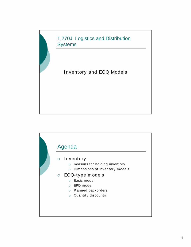
Inventory

inventory supply demand

Inventory = cumulative supply – cumulative demand

Why hold inventories?

{ The transaction motive { Economies of scale: production, transportation,

discount, replenishment, … { Competition purpose

{ The precautionary motive { Demand uncertainty: unpredictable events { Supply uncertainty: lead time, random

yield, … { The speculative motive

{ Fluctuating value: ordering cost, selling price { Demand increase: seasonality, promotion, …

2

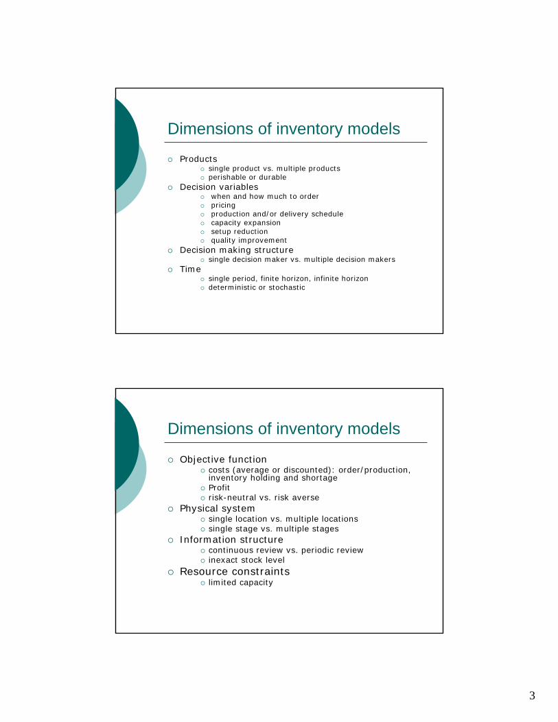
Dimensions of inventory models

{ Products{ single product vs. multiple products{ perishable or durable

{ Decision variables{ when and how much to order{ pricing{ production and/or delivery schedule{ capacity expansion{ setup reduction{ quality improvement

{ Decision making structure{ single decision maker vs. multiple decision makers

{ Time{ single period, finite horizon, infinite horizon{ deterministic or stochastic

Dimensions of inventory models

{ Objective function{ costs (average or discounted): order/production,

inventory holding and shortage{ Profit{ risk-neutral vs. risk averse

{ Physical system{ single location vs. multiple locations{ single stage vs. multiple stages

{ Information structure{ continuous review vs. periodic review{ inexact stock level

{ Resource constraints{ limited capacity

3

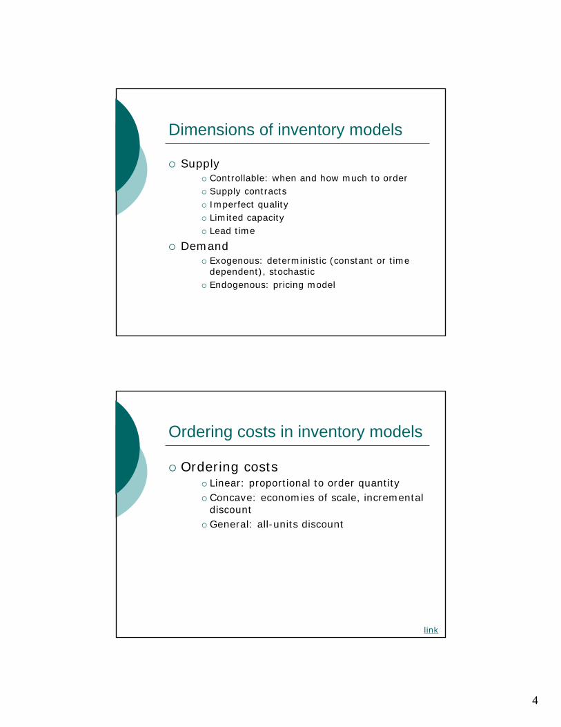
Dimensions of inventory models

{ Supply { Controllable: when and how much to order { Supply contracts { Imperfect quality { Limited capacity { Lead time

{ Demand{ Exogenous: deterministic (constant or time

dependent), stochastic { Endogenous: pricing model

Ordering costs in inventory models

{ Ordering costs { Linear: proportional to order quantity { Concave: economies of scale, incremental

discount{ General: all-units discount

link

4

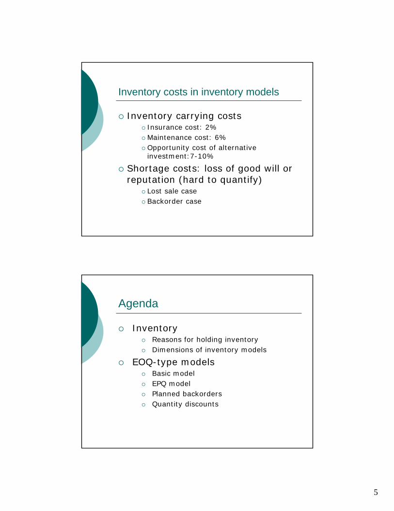
Inventory costs in inventory models

{ Inventory carrying costs { Insurance cost: 2% { Maintenance cost: 6% { Opportunity cost of alternative

investment:7-10%

{ Shortage costs: loss of good will or reputation (hard to quantify)

{ Lost sale case { Backorder case

Agenda

{ Inventory { Reasons for holding inventory { Dimensions of inventory models

{ EOQ-type models { Basic model { EPQ model { Planned backorders { Quantity discounts

5

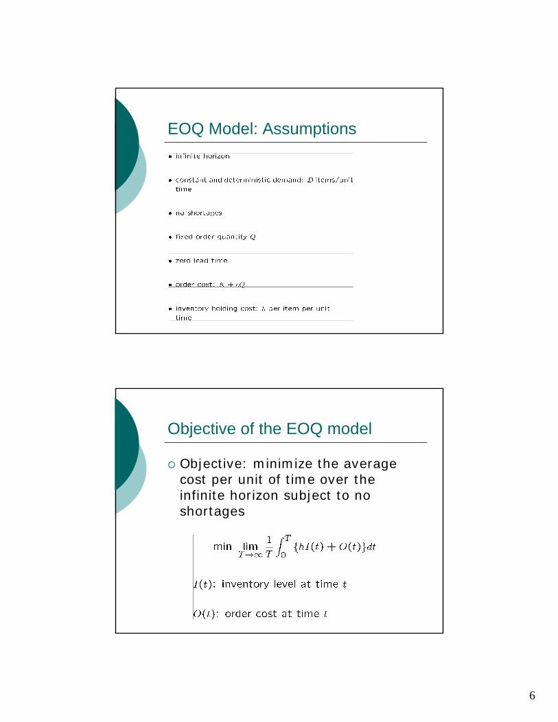
EOQ Model: Assumptions

Objective of the EOQ model

{ Objective: minimize the average cost per unit of time over the infinite horizon subject to no shortages

6

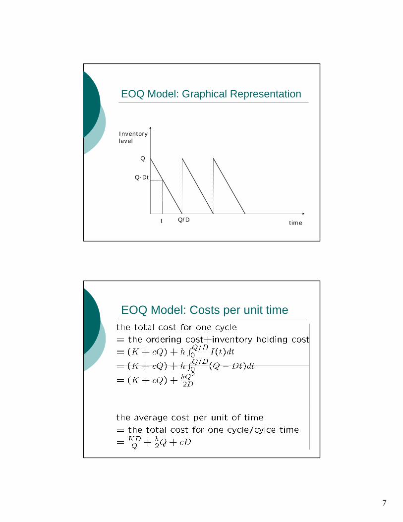
EOQ Model: Graphical Representation

Inventory level

Q

Q-Dt

t Q/D time

EOQ Model: Costs per unit time

7

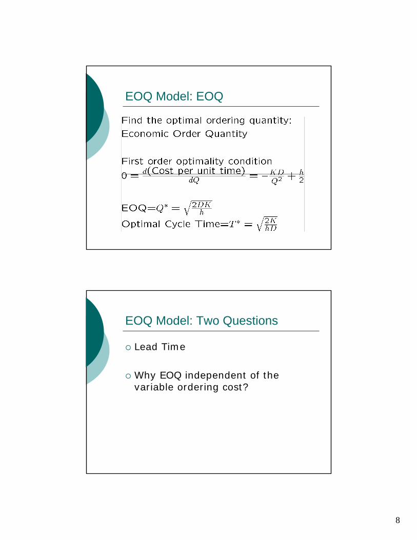
EOQ Model: EOQ

EOQ Model: Two Questions

{ Lead Time

{ Why EOQ independent of the variable ordering cost?

8

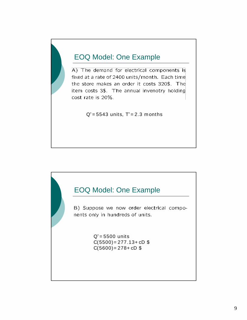
EOQ Model: One Example

Q*=5543 units, T*=2.3 months

EOQ Model: One Example

Q*=5500 units C(5500)=277.13+cD $ C(5600)=278+cD $

9

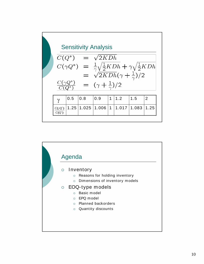
Sensitivity Analysis

1.251.0831.01711.0061.0251.25

21.51.210.90.80.5γ *

*

( )

( )

C Q

C Q

γ

Agenda

{ Inventory { Reasons for holding inventory { Dimensions of inventory models

{ EOQ-type models { Basic model { EPQ model { Planned backorders { Quantity discounts

10

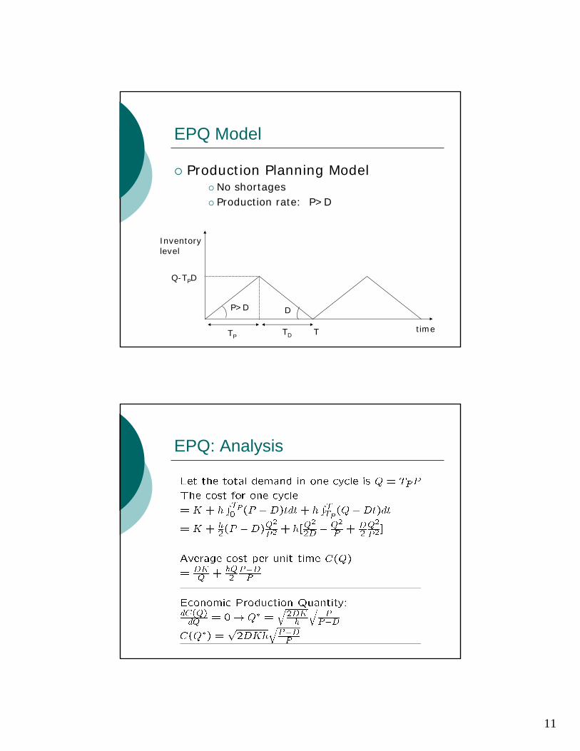
EPQ Model

{ Production Planning Model { No shortages { Production rate: P>D

Inventory level

Q-TPD

P>D D

TP TD T time

EPQ: Analysis

11

Agenda

{ Inventory { Reasons for holding inventory { Dimensions of inventory models

{ EOQ-type models { Basic model { EPQ model { Planned backorders { Quantity discounts

EOQ Model: Planned Backorder

{ Let π be the shortage cost per item per unit of time

Inventory level

s

s-Dt

Q

time

t

(Q-s)/D s/D

12

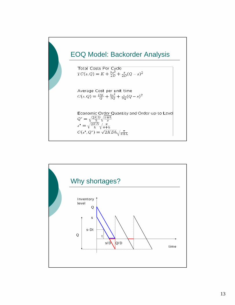
EOQ Model: Backorder Analysis

Why shortages?

Inventory level

time

s

t

Q/D

s-Dt

s/D

Q

Q

13

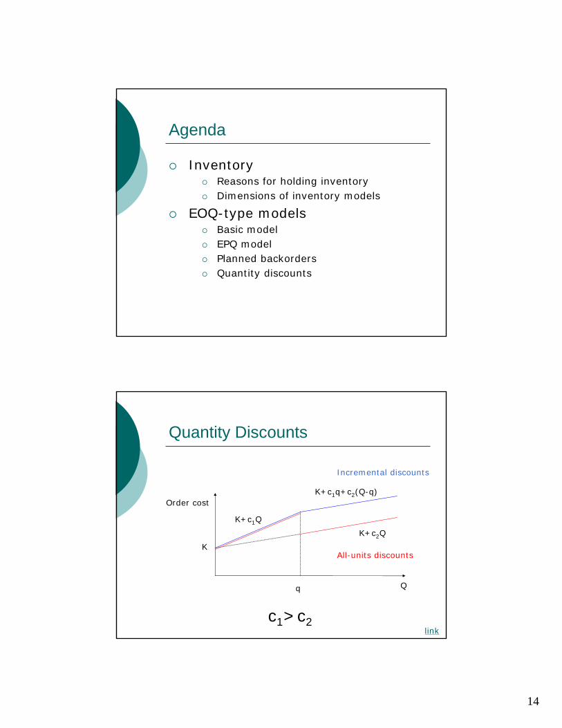
Agenda

{ Inventory { Reasons for holding inventory { Dimensions of inventory models

{ EOQ-type models { Basic model { EPQ model { Planned backorders { Quantity discounts

Quantity Discounts

Incremental discounts

K+c1q+c2(Q-q) Order cost

K+c1Q

K+c2Q

K All-units discounts

Qq

c1>c2 link

14

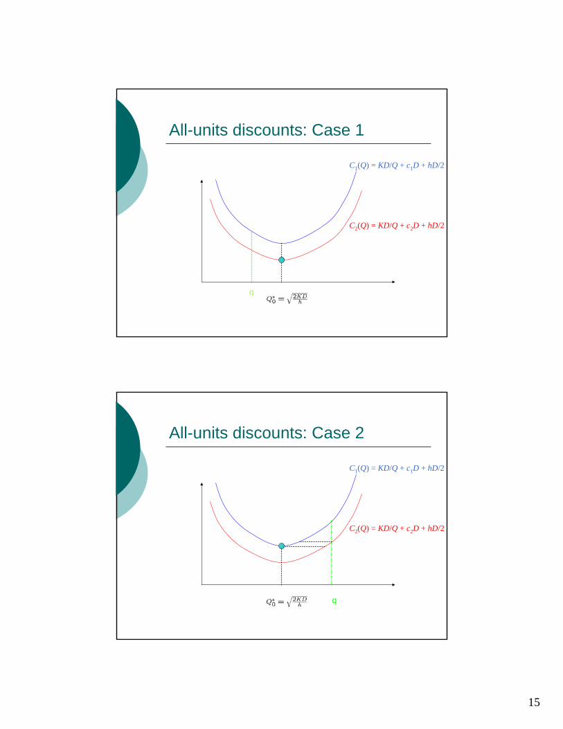
All-units discounts: Case 1

C1(Q) = KD/Q + c1D + hD/2

C2(Q) = KD/Q + c2D + hD/2

q

All-units discounts: Case 2

C1(Q) = KD/Q + c1D + hD/2

C2(Q) = KD/Q + c2D + hD/2

q

15

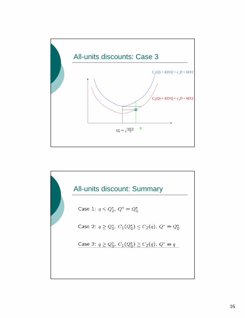
All-units discounts: Case 3

C1(Q) = KD/Q + c1D + hD/2

C2(Q) = KD/Q + c2D + hD/2

q

All-units discount: Summary

16

MIT OpenCourseWarehttp://ocw.mit.edu

ESD.273J / 1.270J Logistics and Supply Chain Management Fall 2009

For information about citing these materials or our Terms of Use, visit: http://ocw.mit.edu/terms.