11.7 Levinson’s Theorem . . . . . . . . . . . . . . . . . . . . . . . . . . . . . . . 278

11.8 Breit-Wigner Resonances . . . . . . . . . . . . . . . . . . . . . . . . . . . . 278

11.9 The Classical Limit . . . . . . . . . . . . . . . . . . . . . . . . . . . . . . . 280

12 Elements of Formal Scattering Theory 283

12.1 Scattering States . . . . . . . . . . . . . . . . . . . . . . . . . . . . . . . . 283

12.2 Properties of the Scattering States . . . . . . . . . . . . . . . . . . . . . . 285

12.3 Integral Equation for ψ(+)~p (~x) . . . . . . . . . . . . . . . . . . . . . . . . . 287

12.4 Coordinate Space Representation of the Lippmann-Schwinger Equation . . 290

12.5 Asymptotic Behavior . . . . . . . . . . . . . . . . . . . . . . . . . . . . . . 293

12.6 The Lippmann-Schwinger Equation as Operator Equation . . . . . . . . . 294

12.7 The Lippmann-Schwinger Equation for the Bound State . . . . . . . . . . 298

12.8 The Low Equation . . . . . . . . . . . . . . . . . . . . . . . . . . . . . . . 299

12.9 Unitarity Relations . . . . . . . . . . . . . . . . . . . . . . . . . . . . . . . 301

12.10S-Operator . . . . . . . . . . . . . . . . . . . . . . . . . . . . . . . . . . . 302

12.11Energy Conservation . . . . . . . . . . . . . . . . . . . . . . . . . . . . . . 303

12.12Unitarity of the S-Operator . . . . . . . . . . . . . . . . . . . . . . . . . . 305

12.13Transition Operator . . . . . . . . . . . . . . . . . . . . . . . . . . . . . . . 306

12.14Cross Section . . . . . . . . . . . . . . . . . . . . . . . . . . . . . . . . . . 308

12.15Scattering of Identical Spinless Particles . . . . . . . . . . . . . . . . . . . 309

12.16The Gellman-Goldberger Relation . . . . . . . . . . . . . . . . . . . . . . . 310

1

Chapter 12

Elements of Formal Scattering

Theory

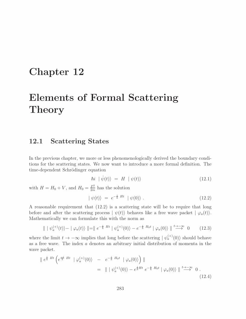
12.1 Scattering States

In the previous chapter, we more or less phenomenologically derived the boundary condi-tions for the scattering states. We now want to introduce a more formal definition. Thetime-dependent Schrodinger equation

~i | ψ(t)〉 = H | ψ(t)〉 (12.1)

with H = H0 + V , and H0 =P 2

2mhas the solution

| ψ(t)〉 = e−i~

Ht | ψ(0)〉 . (12.2)

A reasonable requirement that (12.2) is a scattering state will be to require that longbefore and after the scattering process | ψ(t)〉 behaves like a free wave packet | ϕa(t)〉.Mathematically we can formulate this with the norm as

‖ | ψ(+)a (t)〉− | ϕa(t)〉 ‖=‖ e− i

~Ht | ψ(+)

a (0)〉 − e−i~

H0t | ϕa(0)〉 ‖ t→−∞−→ 0 (12.3)

where the limit t→ −∞ implies that long before the scattering | ψ(+)a (0)〉 should behave

as a free wave. The index a denotes an arbitrary initial distribution of momenta in thewave packet.

‖ e i~

Ht(

e−i~

Ht | ϕ(+)a (0)〉 − e−

i~

H0t | ϕa(0)〉)

‖

= ‖ | ψ(+)a (0)〉 − e

i~Ht e−

i~

H0t | ϕa(0)〉 ‖ t→−∞−→ 0 .

(12.4)

283

Thus, we can define a scattering state as

| ψ(+)a 〉 = s− lim

t→−∞e

i~

Ht e−i~

H0t | ϕa〉 = Ω(+) | ϕa〉 (12.5)

where we defined the Møller operator

Ω(+) := s− limt→−∞

W (t) = s− limt→−∞

ei~

Ht e−i~

H0t . (12.6)

In order to show the existence of the Møller operator, we have to show the convergence.Let t2 < t1 < 0 and consider

‖ [W (t2)−W (t1)] ϕa ‖ = ‖∫ t2

t1

dtdW (t)

dtϕa ‖

≤ |∫ t2

t1

dt ‖ dW (t)

dtϕa ‖ |

= |∫ t2

t1

dt ‖ e i~

Ht 1

~(H −H0) e

− i~

H0t ϕa ‖ |

= |∫ t2

t1

dt1

~‖ V e−

i~

H0t ϕa ‖ |

= |∫ t2

t1

dt1

~‖ V ϕa(t) ‖ | .

(12.7)

The existence of the integral means that the norm ‖ · ‖ has to fall off at least as 1|t|1+ε .

We already showed that a free wave packet decays as 1|t|3/2

. If V only exists in a finite

range, one only has to integrate over a finite region, and then the fall-off in t is sufficient.To show this, let us consider the norm in (12.7) separately.

‖ V ϕa(~r) ‖2 =

∫

d3x V 2(~x) | ϕa(~x, t) |2 (12.8)

We assume that V is square integrable, i.e., a vector in the Hilbert space. If, e.g., Vis local and real, e.g., e−µr/r, this is certainly fulfilled. (V square integrable means∫

d3x V 2(~x) <∞.) Then (12.8) becomes

∫

d3x V 2(~x) | ϕa(~x, t) |2 ≤∫

d3x | V (~x) |2 | ϕa(~x, t) |2

≤∫

d3x V 2(~x)c

t3

=c

t3

∫

d3x V 2(x) =c

t3· c′

(12.9)

284

and thus

‖ V ϕa(~r) ‖ ≤ c

| t |3/2 . (12.10)

For the original estimate (12.7) then follows

|∫ t2

t1

dt1

~‖ V ϕa(t) ‖ | ≤ |

∫ t2

t1

dtc

~

1

| t |3/2 ≤ | 1

| t2 |1/2− 1

| t1 |1/2| t→−∞−→ 0 .(12.11)

Thus, for square-integrable potentials, the Møller operator exists. If V ≡V (~r), thenV ∼ 1

r3/2+ε in order to be square integrable. It can actually be shown (Kupsch-Sandhastheorem) that the Møller operators exist if the potential

| V (~r) | ≤ c

r1+ε(12.12)

for r ≥ R, i.e., falls off for large r faster than the Coulomb potential. We can alwaysexpand a wave packet | ϕa〉 ∈ H with respect to plane waves

| ϕa〉 =

∫

d3p | ~p〉〈~p | ϕa〉 =

∫

d3p | ~p〉 ϕa(~p) . (12.13)

The scattering state is then given by

| ψ(+)〉 = Ω+ | ϕa〉

=

∫

d3p Ω+ | ~p 〉 ϕa(~p)

=

∫

d3p | ~p 〉(+) ϕa(~p)

(12.14)

where we define

Ω(+) | ~p 〉 = | ~p 〉(+) . (12.15)

Here that states | ~p 〉(+) correspond to the scattering states. The distribution functionϕa(~p) is the same for the free wave packet and the scattering state, only the ”basis vectors”change when going to scattering states.

12.2 Properties of the Scattering States

In (12.6) we have defined the Møller operator as limit for t→ −∞ of the operator

W (t) := ei~

Ht e−i~H0t . (12.16)

285

To investigate properties of the Møller operator, we consider

limt→∞

‖ (W (t)− Ω+)ϕ ‖ = limt→∞

(‖ W (t)ϕ ‖ − ‖ Ω+ϕ ‖) = 0 , (12.17)

from which follows (since W (t) unitary)

limt→−∞

‖W (t)ϕ ‖ = ‖ Ω(+)ϕ ‖ = ‖ ϕ ‖ (12.18)

from which we can extract that

〈ϕ | ϕ〉 = 〈Ω(+)ϕ | Ω(+)ϕ〉 = 〈ϕ | (Ω(+))† Ω(+) | ϕ〉 , (12.19)

or since | ϕ〉 is an arbitrary state

(Ω(+))† Ω(+) = 1 . (12.20)

The Møller operator is an isometric operator (preserves the norm); however, it is not aunitary operator, i.e., a left inverse does not exist. Next we consider

(+)〈~p ′ | ~p 〉(+) = 〈Ω(+)~p ′ | Ω(+)~p 〉 = 〈~p ′ | (Ω(+))† Ω(+) | ~p 〉= 〈~p ′ | ~p 〉 = δ(~p ′ − ~p ) .

(12.21)

(12.21) shows that the scattering solutions are normalized to a δ-function in the same waythe plane waves are. For further studying the properties of the states | p〉(+), we rewriteΩ(+) as

Ω(+) = s− limt→−∞

ei~

Ht e−i~

H0t

= s− limt→−∞

ei~

H(t−τ) e−i~

H0(t−τ)

= e−i~

Hτ Ω(+) ei~

H0τ .

(12.22)

Differentiating with respect to τ and evaluating at τ = 0 leads to

0 =i

~HΩ(+) − i

~Ω(+) H0

from which the so-called ”intertwining relation” results:

HΩ(+) = Ω(+) H0 . (12.23)

Applying (12.23) on a plane wave state | ~p〉 givesHΩ(+) | ~p 〉 = Ω(+) H0 | ~p 〉

= Ω(+) P2

2m| ~p 〉

=p2

2mΩ(+) | ~p 〉 ,

(12.24)

286

from which follows

H | ~p 〉(+) =p2

2m| ~p 〉(+) , (12.25)

which states that the full scattering solution | ~p 〉(+) multiplied with H gives the sameenergy as the free solution | ~p 〉 multiplied with H0. This also means that the full solutionbehaves at large distances similar to the free solution, a boundary condition which wejust imposed in the previous chapter. We also showed that | ~p 〉(+) are eigenstates to thefull Hamiltonian H .

Going to the coordinate space representation should give the results of the previous chap-ter. For the free Schrodinger equation, we have

〈~x | H0 | ~p 〉 =

∫

d3x′ 〈~x | H0 | ~x ′〉〈~x ′ | ~p 〉

=

∫

d3x′ 〈~x | − ~2

2m∇2 δ(~x− ~x ′) | ~x ′〉〈~x ′ | ~p 〉

= − ~2

2m∇2 〈~x | ~p 〉 =

p2

2m〈~x | ~p 〉

(12.26)

where 〈~x | ~p 〉 = 1(2π~)3/2

exp(

i~~p · ~x

)

. In a similar fashion, we obtain

〈~x | H | ~p 〉(+) =

(

− ~2

2m∇2 + V

)

〈~x | ~p 〉(+) =p2

2m〈~x | ~p 〉(+) (12.27)

or with 〈~x | ~p 〉(+) = ψ†~p(~x)

(

− ~2

2m∇2 + V

)

ψ†~p(~x) =

p2

2mψ†~p(~x) , (12.28)

which is the stationary Schrodinger equation for positive energies. Again, the eigenstatesare not normalizable. However, here this is a consequence; in the considerations of theprevious chapter it had to be an assumption. We still will have to show that | ~p 〉(+) =Ω(+) | ~p 〉 has the correct asymptotic behavior.

12.3 Integral Equation for ψ(+)~p (~x)

Before being able to set up an integral equation, we have to prove the following statement.Given a function g(t), then for ε > 0

limt→−∞

g(t) = − limε→0

∫ −∞

0

dt′ ε eεt′g(t′) . (12.29)

287

We start from the right-hand side

−∫ −∞

0

dt′ ε eεt′g(t′) = −

∫ −∞

0

d

dt′(eεt

′) g(t′) dt′

= g(0) +

∫ −∞

0

dt′ eεt′ dg(t′)

dt′.

(12.30)

As a remark, the limit and the integral operation can be interchanged if both convergeseparately. Thus we have

limε→0

(−ε)∫ −∞

0

dt′ eεt′g(t′) = lim

ε→0

[

g(0) +

∫ −∞

0

dt′ eεt′ dg(t′)

dt′

]

= g(0) + g(−∞) − g(0)

= g(−∞) .

(12.31)

With this ”Abel Limit”, we replace the limit with respect to t by a limit ε → 0. Nowwe consider the operators

Ω(+) = W (−∞) = − limε→0

∫ −∞

0

ε eεtW (t) dt

= − limǫ→0

∫ −∞

0

ε eεt εi~

Ht e−i~H0t dt

= − limε→0

ε

∫ −∞

0

ei~

Ht e−i~(H0+iε)t dt .

(12.32)

Applying this on a state | ~p 〉 yields

Ω(+) | ~p 〉 = − limε→0

ε

∫ −∞

0

dt ei~

(H−E−iε)t | ~p 〉

= limε→0

εi~(H − E − iε)

| ~p 〉

= limε→0

iε~

E + iε−H| ~p〉 = lim

ε→0iε G(z) | ~p〉

(12.33)

where in the last step ~ ≡ 1 was set and z = E + iε. The function

G(z) =1

z −H(12.34)

288

is called the Resolvent of H . With (12.33) the scattering state can be written as

| ~p 〉(+) = Ω(+) | ~p 〉 = limε→0

iε G(E + iε) | ~p〉 . (12.35)

G(E + iε) contains the full Hamiltonian in the denominator and cannot be treated in theform (12.35). Therefore, we want to split to equation in such a way that H0 and V are inseparate pieces. We define the free Resolvent as

G0(z) =1

z −H0(12.36)

and consider

G−10 (z) − G−1(z) = (z −H0) − (z −H) = −H0 + H = V . (12.37)

Multiplying (12.37) from the left with G0(z) and the right with G(z) gives

G0(z) [G−10 (z) − G−1(z)] G(z)

= G(z) − G0(z) = G0(z) V G(z) ,

from which follows

G(z) = G0(z) + G0(z) V G(z) . (12.38)

The relation (12.38) is called Hilbert identity or Second Resolvent equation, andhas already the typical form of an integral equation. Multiplying (12.37) from the rightwith G0(z) gives a different form of the Hilbert identity, namely

G(z) = G0(z) + G(z) V G0(z) . (12.39)

By comparison of the last terms in (12.38) and (12.39), we find G0(z) V G(z) =G(z) V G0(z). Applying (12.38) on a free state | ~p 〉 gives

G(E + iε) | ~p 〉 = G0(E + iε) | ~p 〉 + G0(E + iε) V G(E + iε) | p〉

iε G(E + iε) | ~p 〉 =iε

E + iε− p2

2m

| ~p 〉 + iε G0(E + iε) V G(E + iε) | ~p 〉 ,

(12.40)

where H0 | ~p 〉 = p2

2m| ~p 〉. Carrying out the lim ε→ 0 gives

limε→0

iε G(E + iε) | ~p 〉 = | ~p 〉(+) = | ~p 〉 + G0(E + i0) V | ~p 〉(+) . (12.41)

Eq. (12.41) is the Lippmann-Schwinger equation for states, and its exists ifV | ~p 〉(+) is a vector out of the Hilbert space, i.e., V is square integrable. The interpre-tation of (12.41) is that the full scattering state | ~p 〉(+) is the sum of an incident plane

289

wave | ~p 〉 and a ”perturbation” G0 V | ~p 〉(+), which is caused by the potential V . Fromthis we can deduce that (12.41) has the form of the boundary condition as postulated in(11.26). Applying the form (12.39) of the Hilbert identity leads to

| ~p 〉(+) = iε G(E + iε) | ~p 〉 = iε [1 +G(E + iε)V ] G0(E + iε) | ~p 〉= [1 +G(E + iε)V ] | ~p 〉= Ω(+) | ~p 〉 ,

(12.42)

from which we deduce a representation of Ω(+) as

Ω(+) = 1 +G(E + iε) V . (12.43)

However, this representation is not very useful since G(E + iε) is not known.

12.4 Coordinate Space Representation of the Lippmann-

Schwinger Equation

For obtaining a coordinate space representation, we have to form

〈~x | ~p 〉(+) = 〈~x | ~p 〉 +

∫

d3x′∫

d3x′′ 〈~x | G0(E + i0) | ~x ′〉〈~x ′ | V | ~x ′〉〈~x ′′ | ~p〉(+)

ψ(+)~p =

1

(2π~)3/2e

i~

~p·~x +

∫

d3x′∫

d3x′′ G(+)0 (~x, ~x ′) V (~x ′, ~x ′′) ψ

(+)~p (~x ′′) .

(12.44)

If V (~x ′, ~x ′′) is assumed to be local, i.e., V (~x ′, ~x ′′) = V (~x ′) δ(~x ′, ~x ′′), this reduces to

ψ(+)~p (~x) =

1

(2π~)3/2e

i~

~p·~x +

∫

d3x′ G(+)0 (~x, ~x ′) V (~x ′) ψ

(+)~p (~x ′) . (12.45)

This is an integral equation, valid for local potentials. The same equation is obtained bysolving the stationary Schrodinger equation.

We still have to determine the coordinate space representation of the free Green function

290

G(+)0 (~x, ~x ′):

G(+)0 = 〈~x | G0(E + i0) | ~x ′〉 = 〈~x | 1

E + i0−H0| ~x ′〉

=

∫

d3p′ 〈~x | 1

E + i0 −H0

| ~p 〉〈| ~p ′ | ~x ′〉

=

∫

d3p′ 〈~x | ~p ′〉〈~p ′ | ~x ′〉 1

E + i0− p′22m

=

∫

d3p′1

(2π~)3e

i~

~p ′·(~x−~x ′) 1

E + i0− p′22m

.

(12.46)

Considering that ~p = ~p ′ and using spherical coordinates leads to

G(+)0 (~x, ~x ′) =

1

(2π~)3

∫ ∞

0

∫ 1

−1

∫ 2π

0

dp p2 d cos θ dϕ ei~

p(x−x′) cos θ 1

E + i0− p2

2m

=m

2π2~2

∫ ∞

0

dp p2e

i~

p(x−x′) − e−i~

p(x−x′)

ip | x− x′ |1

2mE + i0− p2

=m

2π2~2

∫ ∞

−∞

dp p1

2mE + i0− p2e

i~

p(x−x′)

i | x− x′ |

=m

2π2~2

∫ ∞

−∞

dp p1

2mE~2

+ i0− k2eip(x−x′)

i | x− x′ | ,

(12.47)

where we used p = ~k in the last relation. The integrand has poles for positive energiesfor 2mE

~2− ~

2k2 = 0, and the poles are located at

~k1/2 = ±√2mE + iε (12.48)

from which follows

~k1 = +√2mE + iε

~k2 = −√2mE − iε .

(12.49)

291

Im

Re-i

+i

ε

ε2mE 2mE- +

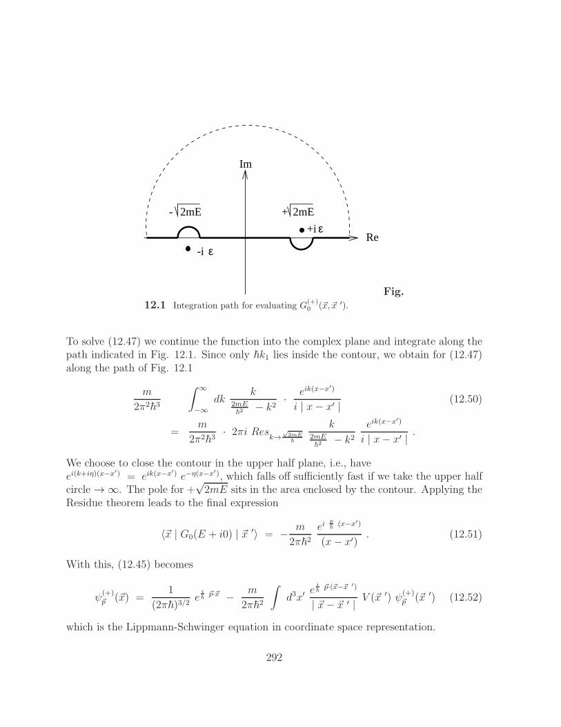
Fig.

12.1 Integration path for evaluating G(+)0 (~x, ~x ′).

To solve (12.47) we continue the function into the complex plane and integrate along thepath indicated in Fig. 12.1. Since only ~k1 lies inside the contour, we obtain for (12.47)along the path of Fig. 12.1

m

2π2~3

∫ ∞

−∞

dkk

2mE~2

− k2· eik(x−x′)

i | x− x′ | (12.50)

=m

2π2~3· 2πi Res

k→√2mE~

k2mE~2

− k2eik(x−x′)

i | x− x′ | .

We choose to close the contour in the upper half plane, i.e., haveei(k+iη)(x−x′) = eik(x−x′) e−η(x−x′), which falls off sufficiently fast if we take the upper halfcircle → ∞. The pole for +

√2mE sits in the area enclosed by the contour. Applying the

Residue theorem leads to the final expression

〈~x | G0(E + i0) | ~x ′〉 = − m

2π~2

eip~

(x−x′)

(x− x′). (12.51)

With this, (12.45) becomes

ψ(+)~p (~x) =

1

(2π~)3/2e

i~

~p·~x − m

2π~2

∫

d3x′e

i~

~p·(~x−~x ′)

| ~x− ~x ′ | V (~x′) ψ

(+)~p (~x ′) (12.52)

which is the Lippmann-Schwinger equation in coordinate space representation.

292

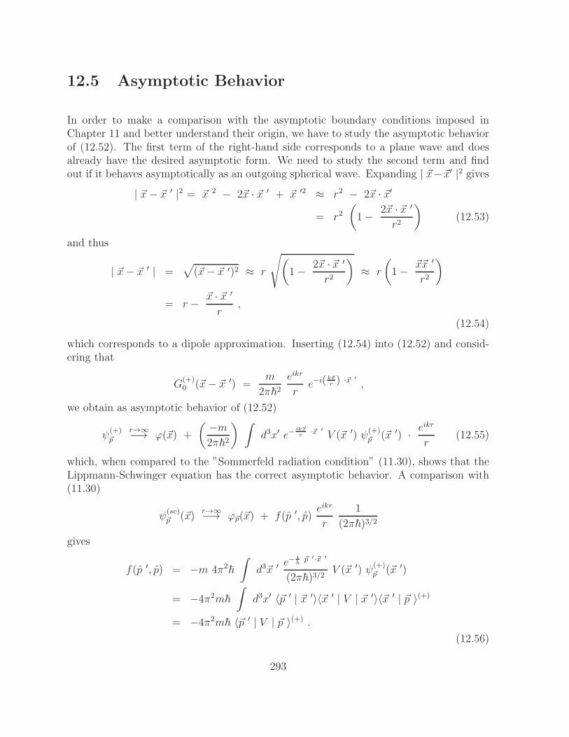
12.5 Asymptotic Behavior

In order to make a comparison with the asymptotic boundary conditions imposed inChapter 11 and better understand their origin, we have to study the asymptotic behaviorof (12.52). The first term of the right-hand side corresponds to a plane wave and doesalready have the desired asymptotic form. We need to study the second term and findout if it behaves asymptotically as an outgoing spherical wave. Expanding | ~x−~x′ |2 gives

| ~x− ~x ′ |2 = ~x 2 − 2~x · ~x ′ + ~x ′2 ≈ r2 − 2~x · ~x′

= r2(

1− 2~x · ~x ′

r2

)

(12.53)

and thus

| ~x− ~x ′ | =√

(~x− ~x ′)2 ≈ r

√

(

1− 2~x · ~x ′

r2

)

≈ r

(

1− ~x~x ′

r2

)

= r − ~x · ~x ′

r,

(12.54)

which corresponds to a dipole approximation. Inserting (12.54) into (12.52) and consid-ering that

G(+)0 (~x− ~x ′) =

m

2π~2

eikr

re−i( k~x

r ) ·~x ′,

we obtain as asymptotic behavior of (12.52)

ψ(+)~p

r→∞−→ ϕ(~x) +

( −m2π~2

)∫

d3x′ e−ik~xr

·~x ′V (~x ′) ψ

(+)~p (~x ′) · eikr

r(12.55)

which, when compared to the ”Sommerfeld radiation condition” (11.30), shows that theLippmann-Schwinger equation has the correct asymptotic behavior. A comparison with(11.30)

ψ(sc)~p (~x)

r→∞−→ ϕ~p(~x) + f(p ′, p)eikr

r

1

(2π~)3/2

gives

f(p ′, p) = −m 4π2~

∫

d3~x ′ e− i

~~p ′·~x ′

(2π~)3/2V (~x ′) ψ

(+)~p (~x ′)

= −4π2m~

∫

d3x′ 〈~p ′ | ~x ′〉〈~x ′ | V | ~x ′〉〈~x ′ | ~p 〉(+)

= −4π2m~ 〈~p ′ | V | ~p 〉(+) .

(12.56)

293

In order to solve for f(p ′, p), one must first solve the Lippmann-Schwinger equation toobtain | ~p 〉(+). Similar to the considerations following (11.91), one can consider solvingfor f(p ′, p ) only in an approximate fashion and expand | ~p 〉(+) =| p〉 + · · · . If oneconsiders only the first term in the expansion, one obtains the Born approximation for

the scattering amplitude

f(p ′, p )Born = −4π2m~ 〈~p ′ | V | ~p 〉 . (12.57)

12.6 The Lippmann-Schwinger Equation as Operator

Equation

In its general form (12.52) can be written as

| ψ(+)~p 〉 = | ϕp〉 + G

(+)0 V | ψ(+)

p 〉 . (12.58)

Multiplying (12.58) with V and defining V | ψ(+)p 〉 = T | ϕp〉 yields

T | ϕp〉 = V | ϕp〉 + V G(+)0 T | ϕp〉 . (12.59)

Since the plane waves | ϕp〉 form a complete set of states, (12.59) is valid as operatorequation:

T = V + V G(+)0 T , (12.60)

which is the Operator Lippmann-Schwinger Equation or t-matrix equation.In its momentum space representation (12.60) reads

〈~p ′ | T | ~p 〉 = 〈~p ′ | V | ~p〉 +

∫

d3p′′ d3p′′′ 〈~p ′ | V | ~p ′′〉〈~p ′′ | G(+)0 | ~p ′′′〉〈~p ′′′ | T | ~p 〉

= 〈~p ′ | V | ~p 〉 +

∫

d3p′′ 〈~p ′ | V | ~p ′′〉 1

E + iε− p′′2

2m

〈~p ′′ | T | ~p 〉 .

(12.61)

This is an integral equation of Fredholm type, and one has to solve for all values of p′′,i.e., off-the-energy-shell. However, one needs for the calculation of physical observablesonly the values for which p′′2

2m= E = p2

2m, i.e., one needs only the on-shell values. The

reason for this is that for the calculation of cross sections only the asymptotic expansionwas used (compared structure of proofs in Chapter 11). The terminology is as follows:Matrix elements for which

p′2 = p2 = p20 are called on− shell ,

294

those for which

p′2 6= p2 = p20 are called half − shell ,

and those for which

p′2 6= p2 6= p20 are called fully − off − shell .

Here p20 is defined via the incoming energy Ep0 =p202m

. In terms of the t-matrix, (12.56)can be written as

f(p ′, p ) = −4π2m~ 〈~p ′ | T | ~p 〉 . (12.62)

Let us consider the propagator G(+)0 in (12.61). If we write it as

〈~p ′ | G(+)0 | ~p 〉 =

δ(~p ′ − ~p )

E + iε− p′2

2m

= δ(~p ′ − ~p )

[

PE − p2

2m

− iπ δ

(

E − p2

2m

)

]

, (12.63)

where we used the Cauchy Principal value

1

x+ iε=

Px

− iπ δ(x) (12.64)

then we can consider the approximation

〈~p ′ | G(+)0 | ~p 〉 ≈ δ(~p ′ − p′)(−iπ) δ

(

E − p2

2m

)

, (12.65)

which is called k-matrix Born approximation.

The Lippmann-Schwinger equation (12.60) is an integral equation of Fredholm type and

can, in principal, be solved by iteration (Neumann series) if the kernel V G(+)0 is small,

so that the convergence of the series is secured. In terms of (12.60), this iteration can bewritten out as

T (1)(z) = V

T (2)(z) = V + V G(+)0 V

T (3)(z) = V + V G(+)0 V G

(+)0 V .

(12.66)

295

In general this series can be written as

T (z) =∞∑

n=1

V (G(+)0 (z)V )n−1 = V

∑

n=0

(G(+)0 (z)V )n (12.67)

and is called Born Series.

We could have also started from the Lippmann-Schwinger equation for states as given in(12.58). If we define as zeroth order to the full solution | ψ(+)

~p 〉0 := | ϕ~p〉, the free solution,then we obtain in first order iteration

| ψ(+)~p 〉1 = | ϕ~p〉 + G

(+)0 V | ϕ~p〉 (12.68)

and in general in n-th order

| ψ(+)~p 〉n =

n∑

ν=0

(G(+)0 V )ν | ϕ~p〉 . (12.69)

If this series converges for n → ∞, we obtain in this way a solution for (12.58), whichreads

| ψ(+)~p 〉 =

∞∑

ν=0

(G(+)0 V )ν | ϕ~p〉 (12.70)

and one can say: If the series (12.70) converges, then the vector defined by the seriesis a proper scattering state. As we have seen in (12.56), the scattering amplitude can bewritten as

fE(p′, p) = −4π2m~ 〈ϕ~p ′ | V | ψ(+)

~p 〉 .

Inserting (12.70) yields

fE(p′, p) = −4π2m~

∞∑

ν=0

〈ϕ~p ′ | V (G(+)0 V )ν | ϕ~p〉 . (12.71)

Thus, the scattering amplitude can be written as a series

fE(p′, p) =

∞∑

i=1

f(i)E (p′, p)

f(i)E (p′, p) = −4π2m~ 〈ϕ~p′ | V (G(+)

0 V )(i−1) | ϕ~p〉 .(12.72)

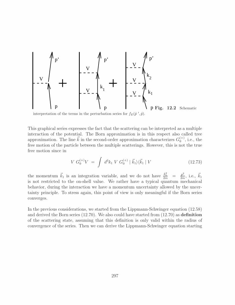
Here (i) counts the power of V . The first Born approximation for the scattering ampli-tude, sometimes called the Born approximation, is linear in the potential. It is useful toconsider a graphical representation of (12.72).

296

V

V

V

V

V

V

p

p’

p

k

p’ p’

p

k

k

1

2

1

Fig. 12.2 Schematic

interpretation of the terms in the perturbation series for fE(p′, p).

This graphical series expresses the fact that the scattering can be interpreted as a multipleinteraction of the potential. The Born approximation is in this respect also called treeapproximation. The line ~k in the second-order approximation characterizes G

(+)0 , i.e., the

free motion of the particle between the multiple scatterings. However, this is not the truefree motion since in

V G(+)0 V =

∫

d3k1 V G(+)0 | ~k1〉〈~k1 | V (12.73)

the momentum ~k1 is an integration variable, and we do not havek212m

= p2

2m, i.e., ~k1

is not restricted to the on-shell value. We rather have a typical quantum mechanicalbehavior, during the interaction we have a momentum uncertainty allowed by the uncer-tainty principle. To stress again, this point of view is only meaningful if the Born seriesconverges.

In the previous considerations, we started from the Lippmann-Schwinger equation (12.58)and derived the Born series (12.70). We also could have started from (12.70) as definitionof the scattering state, assuming that this definition is only valid within the radius ofconvergence of the series. Then we can derive the Lippmann-Schwinger equation starting

297

from (12.70).

| ψ(+)~p 〉 =

∞∑

ν=0

(G(+)0 V )ν | ϕ~p〉

= | ϕ~p〉 + G(+)0 V

∞∑

ν=1

(G(+)0 V )ν−1 | ϕ~p〉

= | ϕ~p〉 + G(+)0 V

∞∑

ν=0

(G(+)0 V )ν | ϕ~p〉

= | ϕ~p〉 + G(+)0 V | ψ(+)

p 〉 .(12.74)

This shows that we ”summed up” the Born series. However, we do not obtain an explicitsolution on the right-hand side, but rather the unknown function again. This indicatesthat in general we do not obtain a closed solution for the scattering state but rather anintegral equation.

We can interpret this in a slightly different way. As we shall see, the Born series con-verges for sufficiently high energies. In that region (12.70) is a reasonable definition andwithin the radius of convergence the Born series and the Lippmann-Schwinger equationare equivalent. This stays valid for all other energies and thus determines the continuationof the definition (12.70) to energy regions, where the series does not exist.

It is appropriate to describe this approach here since it shows how one obtains an integralequation by summing up multiple interactions of V . This procedure is important withrespect to quantum field theory. There the usual practice leads to a Dyson series (aninfinite series corresponding to the Born series, represented by Feynman diagrams).

Summing up this series gives an integral equation, which resembles in its form theLippmann-Schwinger equation, the Bethe-Salpeter equation, which, however, has amuch more complicated structure.

12.7 The Lippmann-Schwinger Equation for the Bound

State

If we assume that V supports a bound state | ψb〉 at E = Eb < 0, then the Schrodingerequation reads

(H0 + V ) | ψb〉 = Eb | ψb〉 (12.75)

298

or

(H0 −Eb) | ψb〉 = −V | ψb〉 . (12.76)

Since Eb < 0, there is no regular solution for the case V = 0 and we can write

| ψb〉 =1

Eb −H0V | ψb〉 , (12.77)

which is the homogeneous Lippmann-Schwinger equation for | ψb〉. Evaluating the freeGreen’s function for E = Eb < 0 (12.51), we see that 〈~x | ψb〉 ≡ ψb(~x ) has the correct

exponential fall-off behavior, namely proportional to e−√

2m|Eb| |x−x′||x−x′|

.

12.8 The Low Equation

When deriving the Lippmann-Schwinger equation for states or operators, we started fromthe Hilbert identity given by (12.38). Now we want to start from the alternative form(12.39), namely

G(z) = G0(z) + G(z) V G0(z) .

Similar to Section 12.3, we apply (12.39) on a free state | ~p 〉, multiplying with iε andconsider the limit ε→ 0.

iε G(E + iε) | ~p 〉 =iε

E + iε− p2

2m

| ~p 〉 + G(E + iε) Viε

E + iε p2

2m

| ~p 〉 . (12.78)

Taking the limit ε → 0 gives

| ~p 〉(+) = | ~p 〉 + G(E + iε) V | ~p 〉 , (12.79)

which is the Low equation for states (corresponding to (12.41)). Multiplying with Vand taking into account the definition V | p〉(+) = T | p〉 gives

V | ~p 〉(+) = T | p〉 = (V + V G V ) | ~p 〉 (12.80)

or as operator equation

T = V + V G V . (12.81)

For practical calculations, the Low equation is not particularly useful, since it containsthe full resolvent G(z). If we assume that the Hamiltonian H has bound states with

299

H | ψb〉 = Eb | ψb〉 and a continuous spectrum, then we can write the spectral decompo-sition of G(z) as

1

E ± iε −H=

∑

b

| ψb〉1

E ± iε−Eb〈ψb |

+

∫

d3p | ψ(+)~p 〉 1

E ± iε−H〈ψ(+)

~p | .

(12.82)

G(z) is a holomorphic function for Im 6= 0, and G(z) has poles at the binding energiesEb. Inserting (12.82) into (12.81) leads to

〈~p ′ | T | ~p 〉 = 〈~p ′ | V | ~p 〉 +∑

b

〈~p ′ | V | ψb〉〈ψb | V | ~p 〉E − Eb

+

∫

d3k〈~p ′ | T † | ~k 〉〈~k | T− | ~p 〉

E ± iε− Ek,

(12.83)

where the subscript ± refers to ±iε in G(E ± iε). If E > 0, then there are no boundstates and the discrete sum over b vanishes. If E < 0 is allowed, then 〈~p ′ | T | ~p 〉 haspoles by E = Eb, and the residue is separable. [Remark: A function f(~q ′, ~q ) is calledseparable if f(q′, q) = f1(q

′) f2(q).] The residue can be written as

〈~p ′ | V | ψb〉 = 〈~p ′ | (H −H0) | ψb〉 = (E − E~p )〈~p ′ | ψb〉= (E − E~p ) ψb(~p

′) ,

(12.84)

where ψb(~p′) is the bound state wave function for E = Eb. Thus, if E < 0 is close to

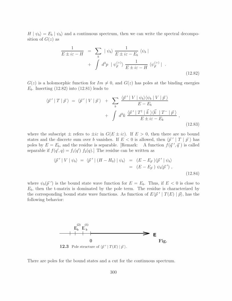
Eb, then the t-matrix is dominated by the pole term. The residue is characterized bythe corresponding bound state wave functions. As function of E〈~p ′ | T (E) | ~p〉, has thefollowing behavior:

EE(1)

b b

E0

(2)

Fig.

12.3 Pole structure of 〈~p ′ | T (E) | ~p 〉.

There are poles for the bound states and a cut for the continuous spectrum.

300

12.9 Unitarity Relations

When considering only positive energies, the sum over b vanishes in (12.83). Let usconsider the difference of T (+) and T (−) as obtained from (12.83) under the assumptionthat V is hermitian.

〈~p′ | T (+)(E) −T (−)(E) | ~p〉 = 〈~p′ | T (+)(E) | ~p〉 − 〈~p′ | T (−)(E) | ~p〉

=

∫

d3k〈~p′ | T (+)(E) | ~k〉[

1

E −Ek + iε− 1

E − Ek − iε

]

〈~k | T (−)(E) | ~p〉.

(12.85)

Using the Cauchy principal value 1x±iε

= Px

∓ iπδ(x), we obtain

〈~p′ | T (+)(E) −T (−)(E) | ~p 〉 (12.86)

= −2πi

∫

d3k〈~p′ | T (+)(Ek) | ~k〉δ(E − Ek)〈~k | T (−)(Ek) | ~p〉

= −2πi

∫ ∞

0

dk k2∫

dΩk〈~p′ | T (+)(Ek) | ~k〉δ(k′′ − k)m

k〈~k | T ()(Ek) | ~p〉

(12.87)

In the last relation we used δ(ax) = 1|a|δ(x), δ(ϕ(x))] =

∑

i1

|ϕ′(ai)|δ(x − ai), where ai are

the roots of the equation ϕ(x) = 0, and E = p′′2

2m.

Eq. (12.87) is called the off-shell unitarity relation, since in general | ~p |6=| ~p ′ |6=| ~k |.

For elastic scattering, i.e., | ~p |=| ~p′ |, Eq. (12.87) simplifies to

〈~p′ | T (+)(Ep) − T (−)(Ep) | ~p 〉 (12.88)

= −2πi m p

∫

dΩk〈~p ′ | T (+)(Ep) | ~k 〉〈~k | T (−)(Ep) | ~p 〉

which is usually referred to as on-shell unitarity relation.

If we restrict ourselves to the forward direction, i.e., ~p ′ = ~p, or equivalently θ = 0, withθ being the angle between ~p ′ or ~p, we obtain

〈~p | T (+)(E) − T (−)(E) | ~p 〉 = 〈~p | T (+) | ~p 〉 − 〈~p | T (+) | ~p 〉∗= 2i Im 〈~p | T (+) | ~p 〉

(12.89)

301

and with (12.89)

Im 〈~p | T (+)(E) | ~p 〉 = −π mp∫

dΩk | 〈~p | T (+)(E) | k〉 |2 . (12.90)

Eq. (12.90) is referred to as optical theorem and provides a non-linear relation betweenthe imaginary part of T in forward direction and the absolute value of T integrated overall angles.

12.10 S-Operator

In (12.4) the scattering state was defined via its behavior for large negative times, i.e.,long before the scattering event.

| ψ(+)a 〉 = s− lim

t→−∞eiHt e−iH0t | ϕa〉 = Ω(+) | ϕa〉 .

In order to completely characterize the scattering event, we need to have the behavior of| ψ(+)

a 〉 for large positive t, i.e.,

| ψ(+)a (t)〉 = e−iHt | ψ(+)

a (0)〉 = e−iHtΩ(+) | ϕa〉 . (12.91)

One of the basic boundary condition was that long after the scattering, the state | ψ(+)a (t)〉

should again behave as a free wave. Thus, in order to characterize the scattering, we shouldconsider the probability coefficients | 〈ϕb(t) | ψa

(+)(t) |2 for large times t. Here | ϕb(t)〉 isa free wave.

Define

Sab = limt→−∞

〈ϕb(t) | ψ(+)a (t)〉

= limt→∞

〈e−iH0t ϕb | e−iHt ψ(+)a 〉

= limt→∞

〈eiHt e−H0t ϕb | ψ(+)a 〉

= 〈Ω(−) ϕb | ψ(+)a 〉 = 〈ψ(−)

b | ψ(+)a 〉

(12.92)

with

Ω(−) := limt→∞

eiHt e−iH0t (12.93)

and

Ω(−) | ϕb〉 := | ψ(−)b 〉 (12.94)

302

which characterizes the outgoing scattering state. The existence of Ω(−) is guaranteed,since the proofs of Section 12.1 never explicitly used the limit t→ ∞. Thus, the transitionprobability from an incoming state to an outgoing state is given by

S2ab = | 〈ψ(−)

b | ψ(+)a |2 . (12.95)

With

Sab = 〈ψ(−)b | ψ(+)

a 〉 = 〈Ω(−) ϕb | Ω(+) ϕa〉= 〈ϕb | Ω(−)† Ω(+) | ϕa〉 := 〈ϕb | S | ϕa〉

(12.96)

we define the scattering operator (S-matrix)

S = Ω(−)† Ω(+) . (12.97)

Using the explicit definition of the Møller operators, it can be easily seen that S is unitary.Furthermore, the existence of S depends on the existence of the Møller operators.

12.11 Energy Conservation

In (12.23) the intertwining relation was given as

HΩ(±) = Ω(±) H0 .

Its complex conjugate equation reads

(Ω(±))† H = H0 Ω±† .

From the isometry property of the Møller operators, Ω(±)† Ω(±) = 1, follows

(Ω(±))† H Ω(±) = H0 . (12.98)

The last equation leads to the interpretation that Ω(±) can be considered as an operatorwhich transforms H into H0. From this point of view, we have to conclude that Ω(±)

cannot be unitary. If it would be, then H and H0 would have to have the same spectrum.

303

Since H0 has only a continuous spectrum, H could not have bound states, which is clearlynot the case. We can say that Ω(±) is then and only then unitary, if H does not havebound states.

Let us consider

SH0 = Ω(−)† Ω(+) H0 = Ω(−)† H Ω(+)

= H0 Ω(−)† Ω(+) = H0S ,

(12.99)

which shows that [S,H0] = 0. We also have

H0 | ~p 〉 = Ep | ~p 〉SH0 | ~p 〉 = Es S | ~p 〉 = H0S | ~p〉 , (12.100)

which means that | ~p 〉 as well as S | ~p 〉 are eigenstates of H0 with the same eigenvalueEp. For the expectation values for H0 in the initial state (before the scattering) and thefinal state (after the scattering), we find

〈ψ(−)b | H0 | ψ(−)

b 〉 = 〈Sψ(+)a | H0 | Sψ(+)

a 〉= 〈ψ(+)

a | S†H0S | ψ(+)a 〉

= 〈ψ(+)a | S†S H0 | ψ(+)

a 〉= 〈ψ(+)

a | H0 | ψ(+)a 〉

(12.101)

H0 has a complete spectrum of non-normalizable eigenstates | ~p 〉, thus S can berepresented in these states. From [S,H0] = 0 follows

0 = 〈~p ′ | [H0, S] | ~p 〉 = 〈~p ′ | H0S | ~p 〉 − 〈~p ′ | SH0 | ~p 〉= (Ep′ − Ep)〈~p ′ | S | ~p 〉 .

(12.102)

From this follows that 〈~p ′ | S | ~p 〉 6= 0 only if Ep′ = Ep. Therefore, we can write

Sp′p = 〈~p ′ | S | ~p 〉 = δ(Ep′ − Ep)〈p′ | S | p〉 (12.103)

where p = ~p/ | ~p |. This means Sp′p is defined on-shell.

304

12.12 Unitarity of the S-Operator

In order to show that S as defined in (12.97) is unitary, we have to show that

S†S = SS† = 1 . (12.104)

The first relation is easy and we use that Ω(+)† Ω(±) = 1:

〈Ω(±)ϕ | Ω(±)ϕ〉 = limt′→∓∞

limt→∓∞

〈eiHt′ e−iH0t′ ϕ | eiHt e−iH0t ϕ〉t′=t= lim

t→∓∞〈eiHt e−iH0t ϕ | eiHt eiH0t ϕ〉

= 〈ϕ | 1 | ϕ〉 = ‖ ϕ ‖2 .

(12.105)

In order to show the other relation, we need to consider the mapping properties of Ω(±)†.Applied on a scattering state, it gives

Ω(±)† | ψ(±)a 〉 = Ω(±)† Ω(±) | ϕa〉 = | ϕa〉 . (12.106)

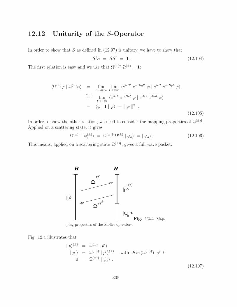
This means, applied on a scattering state Ω(±)†, gives a full wave packet.

|p>

|p>

b

(+)

(+)

(+)

Ω

Ω

H H

|ψ >Fig. 12.4 Map-

ping properties of the Møller operators.

Fig. 12.4 illustrates that

| p〉(±) = Ω(±) | ~p 〉| ~p 〉 = Ω(±)† | ~p 〉(±) with Ker(Ω(±)†) 6= 0

0 = Ω(±)† | ψn〉 .(12.107)

305

Thus Ω(±) Ω(±)† = Pc, a projection operator on the continuous spectrum. Now consider

S†S = (Ω(−)†Ω(+))†(Ω(−)†Ω(+)) = Ω(+)†Ω(−)Ω(−)† Ω(+)

= Ω(+)† PcΩ(+) = 1

SS† = (Ω(−)†Ω(+))(Ω(−)†Ω(+))† = Ω(−)†Ω(+)Ω(+)†Ω(−)

= Ω(−)†Pc Ω(−) = 1 .

(12.108)

As a remark: S is only unitary on the whole Hilbertspace H if the states | p〉(+) spanthe entire space of scattering states.

Let us now consider the probability of scattering into all possible final states

∫

d3p | 〈~p | S | ϕa〉 |2 =

∫

d3p 〈~p | S | ϕa〉∗〈~p | S | ϕa〉

=

∫

d3p 〈ϕa | S† | ~p 〉〈~p S | ϕa〉

= 〈ϕa | S†S | ϕa〉 = ‖ ϕa ‖2 .

(12.109)

Thus, the probability is conserved in the scattering process.

12.13 Transition Operator

In (12.96) the scattering operator was defined as the transition probability

Sba = 〈ψ(−)b | ψ(+)

a 〉

= 〈ϕb | ψ(+)a 〉 + 〈 1

Ea − iε−HV ϕb | ψ(+)

a 〉 ,

(12.110)

where we used the Low equation (12.79) for the last step. One also has

〈ϕb | ψ(+)a 〉 = 〈ϕb | ϕa〉 + 〈ϕb | G0(Ea + iε) V | ψ(±)

a 〉 .

= δba +1

Ea − Eb − iε〈ϕb | V | ψ(+)

a 〉

(12.111)

306

Inserting (12.111) into (12.110) leads to

Sba = δba +

[

1

Eb −Ea + iε− 1

Eb −Ea − iε

]

〈ϕb | V | ψ(+)a 〉

= δba − 2πi δ(Eb − Ea) 〈ϕb | T (+)(Ea) | ϕa〉= δba − 2πi δ(Eb − Ea) T

(+)ab (Ea) .

(12.112)

This suggests that the S operator can be split into two parts according to

S = 1 − 2πi τ (+) (12.113)

where

τ(±)ba := δ(Eb −Ea) T

(±)ba (12.114)

describes the scattering. For the interaction V = 0 follows S = 1.

Thus, τ±ba describes the scattering process and has to appear in the differential crosssection. Thus for scattering relevant quantity is S − 1, where the scattering in forwarddirection is subtracted. Due to the δ function δ(Eb−Ea), τ

(±)ba is only defined for Eb = Ea,

i.e., on-shell. Another way to formulate this is that the S operator only defines the on-shell elements of the T operator. However, this is not enough to define an operator – onehas to know the matrix elements for all momenta. From the unitarity of the S operatorfollows

SS† = (1− 2πiτ (+))(1+ 2πiτ (−))

= 1− 2πi(τ (+) − τ (−)) + 4π2 τ (+)τ (−)

(12.115)

and from there

τ (+) − τ (−) = −2πi τ (+)τ (−)

δ(Eb − Ea)(T(+)ba − T

(−)ba ) = −2πi

∑

α

δ(Eb −Ea) δ(Ea −Eα) T(+)bα T (−)

αa

(12.116)

and for E0 = Ea

T(+)ba − T

(−)ba = −2πi

∑

α

δ(Eb − Eα) T(+)bα T (−)

αa (12.117)

307

or explicitly

〈~p | T+(Ep)− T (−)(Ep) | ~p 〉 = −2πi

∫

d3k δ(Ep − Eα)

〈~p | T (+)(Ep) | ~k 〉〈~k | T (−)(Ep) | ~p 〉(12.118)

which is the on-shell unitarity relation already derived in (12.89). However, (12.118)contains less information than the unitarity relations derived in Section 12.9, which aregiven fully-off-shell.

12.14 Cross Section

The cross section should describe the probability that under given initial conditions some-thing is scattered into the direction of ~p ′, where the forward direction should be sub-tracted. This probability is obviously given by S − 1 and can be defined as

dW = d3p′ | −2πi〈~p ′ | T | ϕ~p 〉 |2= p′2 dp′ dΩ~p ′ | −2πi〈~p ′ | T | ϕ~p 〉 |2

= m√2mE ′ dE ′ dΩ~p 4π2 | 〈~p ′ | T | ϕ~p 〉 |2

(12.119)

where p2 = 2mE has been used. Next we need to consider

| 〈~p ′ | T (Ep) | ϕ~p 〉 |2 =

∣

∣

∣

∣

∫

d3p 〈~p ′ | T (Ep) | ~p 〉 ϕp0(~p )

∣

∣

∣

∣

2

=

∣

∣

∣

∣

∫

d3p δ(E ′ −Ep)〈p′ | T (Ep) | p〉 ϕp0(~p )

∣

∣

∣

∣

2

.

(12.120)

For ϕp0(~p ) being a wave packet which is sharply peaked at ~p = ~p0 and 〈p′ | T (Ep) | p〉being a slowly varying function, we can write

|〈~p ′ | T (Ep) | ϕ~p 〉 |2 ≃ | 〈p′ | T (Ep0) | p〉 |2∫

d3p δ(E ′ − Ep) ϕp0(~p ) |2

and thus

dW ≈ 4π2 mp0 dΩ dE | 〈p′ | T (Ep0) | p〉 |2∫

d3p δ(E ′ − Ep) ϕp0(~p ) |2

= 4π2 mp0 dΩ dE | 〈p′ | T (Ep0) | p〉 |2 I(Ep) .

(12.121)

308

Needed is the scattering into a definite solid angle dΩ, thus one can integrate over theenergy

dW (Ω) = 4π2 mp0 dΩ | 〈p′ | T (Ep0) | p0〉2∫

dE ′ I(E) . (12.122)

The energy δ-function can be written asδ(E ′ − E) = m

p0δ(| ~p′ | − | ~p0 |) leading to another factor m

p0in 12.122.

The differential cross section was defined as the flux scattered into a specific solid angledΩ divided by the incoming flux:

dσ =dW (Ω)

W0

=(2π)4 mp0 · m

p0ρ0 ∆t | 〈p′ | T (Ep0) | pa |2 dΩ

ρ0 ∆t

(12.123)

from which follows

dσ

dΩ= (2π)4 m2 | 〈p′ | T (Ep0) | p0〉 |2 = | f(p′, p) |2 (12.124)

which gives the relation between the on-shell t-matrix and the scattering amplitude. Forthe total cross section this leads to

σtot =

∫

dΩdσ

dΩ= (2π)4m2

∫

dΩ|〈p′|T (Ep0)|p〉|2. (12.125)

12.15 Scattering of Identical Spinless Particles

For identical particles the states have to be symmetric (or antisymmetric) under theexchange of the two particles. Interchanging particle labels corresponds to replacing~p = (p, θ, φ) by −~p = (p, π − θ, φ + π). Similarly, the scattering amplitude has to besymmetric (antisymmetric) under the exchange of 1 and 2, i.e., we have to consider

f(p′, p) ± f(−p′, p) = f(θ, φ) ± f(π − θ, φ+ π) , (12.126)

Since for spinless particles, the interaction is rotationally invariant around the axis alongthe incoming momentum ~p, we drop the dependence on φ and have

dσ

dΩ= | fp(θ) + fp(π − θ) |2

= | fp(θ) |2 + | fp(π − θ) |2 + 2Re(f ∗(θ) f(π − θ)) .

(12.127)

309

First, the differential cross section for the scattering of two identical spinless particlesis symmetric around 90o. Second, dσ

dΩcontains three terms, the cross sections for the

amplitudes for scattering into the direction (θ, φ) for particles interference from z = −∞and z = +∞ and an influence term, which is a typical quantum mechanical effect, sinceone must add amplitudes and not intensities.

Next, we consider the scattering of two identical spin 12particles interacting via a spin-

independent potential. Since their spin is a good quantum number, we consider S = 0 andS = 1 states separately. The total wave function must be antisymmetric. For S = 0, χs=0

is antisymmetric, thus the spatial part must be symmetric. Thus, we obtain for the crosssection in the singlet state

dσsdΩ

= | f(θ) + f(π − θ) |2 (12.128)

For S = 1, χs=1 is symmetric, thus the spatial part must be antisymmetric, and we obtain

dσtdΩ

= | f(θ) − f(π − θ) |2 . (12.129)

Eqs. (12.128) and (12.129) assume that the scattering particles are in a definite spinstate, i.e., beam and target are polarized. If this is not the case, i.e., if beam as well astarget are unpolarized, i.e., spins are randomly oriented, then we must average over therandom spin orientations. This corresponds to the assumption that the four spin states,S = 0, ms = 0, S = 1, ms = ±1, 0 occur with equal frequency. Then the unpolarized

differential cross section is given by

dσ

dΩ(unpol) =

1

4

dσsdΩ

+3

4

dσtdΩ

. (12.130)

12.16 The Gellman-Goldberger Relation

The Gellman-Goldberger relation or two-potential formula is particularly appropriatewhen the interaction between the projectile and the target decomposes naturally into twoparts: V = V0 + V1. This division is especially useful if the scattering wave functionunder the action of one part can be obtained exactly, while the effect of the other canbe treated in the same approximation. In this sense, the formula leads to the so-called”distorted-wave Born approximation” and, in other circumstances, to the method of the”final state interaction.”

Let us assume that the interaction potential V = V0 + V1. Then, the corresponding LSequation reads

T = (V0 + V1) + (V0 + V1) G0T

= (V0 + V1) + V0 G0T + V1 G0T (12.131)

310

As a reminder, from (12.58) we had for the scattering state

| ~p 〉(+) = | ~p 〉 + G0V | ~p 〉(+)

from which follows

| ~p 〉(+) = (1−G0V )−1 | ~p 〉 = Ω(+) | ~p 〉 . (12.132)

From the relation (12.39), we obtained the Low equation in the form

| ~p 〉(+) = | ~p 〉 + GV | ~p 〉 = (1 +GV ) | ~p 〉 = Ω(+) | p〉 (12.133)

So we have the different representations of the Møller operator

Ω(+) = (1−G0V )−1 = (1 +GV ) = 1 + G0T . (12.134)

Multiplying (12.131) from the left with Ω(+)†0 := (1− V0G0)

−1 gives

(1− V0G0)−1 (1− V0G0)T = (1− V0G0)

−1 V0 + (1− V0G0)−1 V1 (12.135)

+ (1− V0G0)−1 V1G0T

T = T0 + (1− V0G0)−1 V1 (1 +G0T )

(12.136)

where we used that T0 = V0 + V0 G0T0 as exact solution of the Hamiltonian H0 + V0.Using the relations (12.134), one obtains

T = T0 + Ω(−)†0 V1 Ω(+) (12.137)

where Ω(+) is the Møller operator for the full scattering problem. Eq (12.137) is the so-called ”two-potential formula.” The first term is the scattering amplitude for the potentialV0 alone; in many cases, it is either known or calculable. The second term incorporatesthe effect of the ”residual potential ”V1 and must often be treated approximately. If theinteraction V1 is sufficiently weak, it can be treated in a first order approximation, whichmeans here Ω(+) ≈ Ω

(+)0 so that

T ≈ T0 + Ω(−)†0 V1 Ω

(+)0 (12.138)

311

or in terms of matrix elements

〈~p ′ | T | ~p 〉 := Tfi = 〈~p ′ | T0 | ~p 〉 + (−)〈~p0 ′ | V1 | ~po〉(+) . (12.139)

The second term is a generalization of the Born approximation in which distorted wavefunctions | p0〉(+) are used to calculate the scattering due to V1 in the presence of V0. It isoften called the distorted wave Born approximation. For instance, in the scatteringof protons from nuclei, one might choose V0 to be the Coulomb potential and V1 the short-range nuclear force. Then the second term in (12.139) approximates the scattering due tothe nuclear force, taking account of the Coulomb repulsion and the consequent reductionin the amplitude of the wave function at small separations. See Ch. Elster, L. C. Liuand R. M. Thaler, “A Practical calculational method for treating Coulomb scattering inmomentum space,” J. Phys. G 19, 2123 (1993).

312