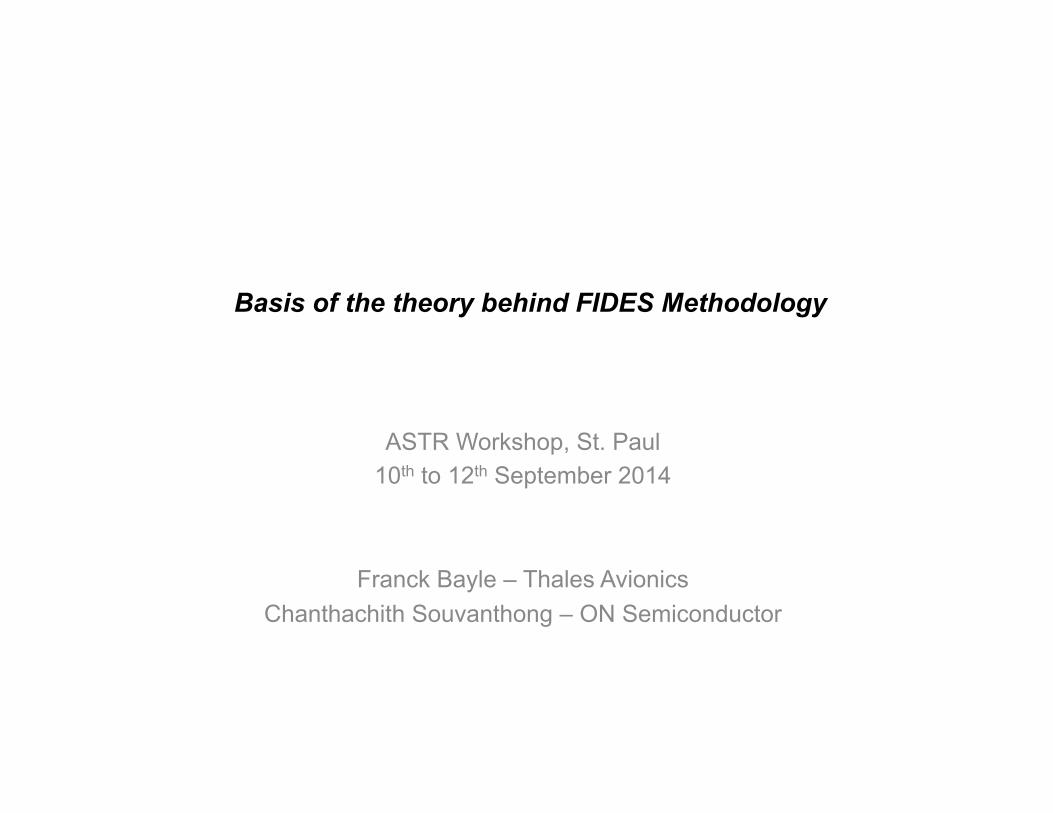
Basis of the theory behind FIDES Methodology

ASTR Workshop, St. Paul 10th to 12th September 2014

Franck Bayle – Thales Avionics Chanthachith Souvanthong – ON Semiconductor

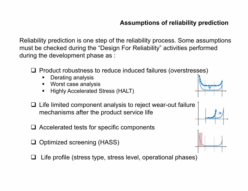
Assumptions of reliability prediction

Reliability prediction is one step of the reliability process. Some assumptions must be checked during the “Design For Reliability” activities performed during the development phase as :

q  Product robustness to reduce induced failures (overstresses) §  Derating analysis §  Worst case analysis §  Highly Accelerated Stress (HALT)

q  Life limited component analysis to reject wear-out failure mechanisms after the product service life

q  Accelerated tests for specific components

q  Optimized screening (HASS)

q  Life profile (stress type, stress level, operational phases)

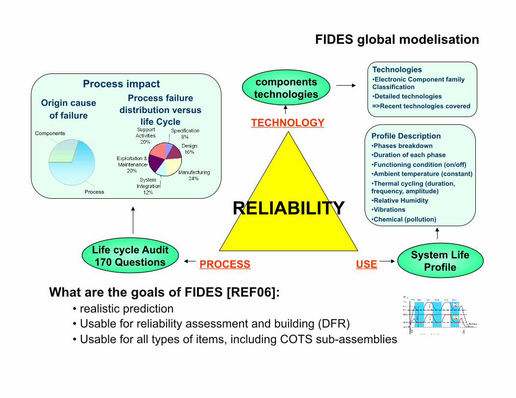
RELIABILITY

TECHNOLOGY

PROCESS USE

What are the goals of FIDES [REF06]: •  realistic prediction •  Usable for reliability assessment and building (DFR) •  Usable for all types of items, including COTS sub-assemblies

Life cycle Audit 170 Questions

components technologies

System Life Profile

Technologies • Electronic Component family Classification • Detailed technologies =>Recent technologies covered

Profile Description • Phases breakdown • Duration of each phase • Functioning condition (on/off) • Ambient temperature (constant) • Thermal cycling (duration, frequency, amplitude) • Relative Humidity • Vibrations • Chemical (pollution)

Process

Components

Origin cause of failure

Process failure distribution versus

life Cycle

Process impact

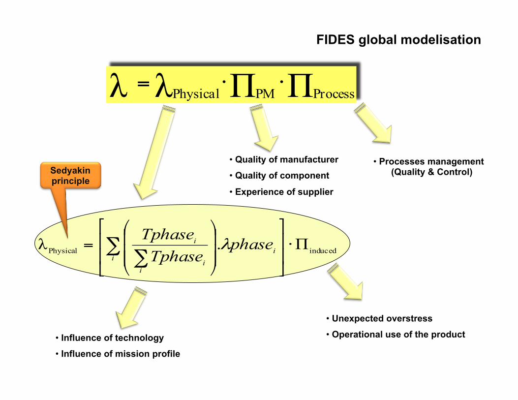
FIDES global modelisation

FIDES global modelisation

ΠΠλλ ProcessPMPhysical ⋅⋅=

•  Unexpected overstress

•  Operational use of the product

•  Quality of manufacturer

•  Quality of component

•  Experience of supplier

•  Processes management (Quality & Control)

inducedPhysical Π.λ ⋅⎥⎥

⎦

⎤

⎢⎢

⎣

⎡

⎟⎟⎟

⎠

⎞

⎜⎜⎜

⎝

⎛= ∑

∑ii

ii

i phaseTphaseTphase

λ

•  Influence of technology

•  Influence of mission profile

Sedyakin principle

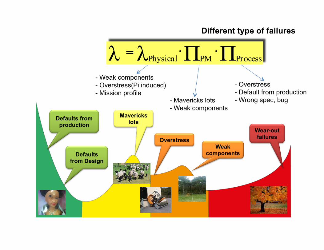
Different type of failures

Defaults from production

Defaults from Design

Wear-out failures

Weak components

Overstress

Mavericks lots

ΠΠλλ ProcessPMPhysical ⋅⋅=

- Overstress - Default from production - Wrong spec, bug - Mavericks lots

- Weak components

- Weak components - Overstress(Pi induced) - Mission profile

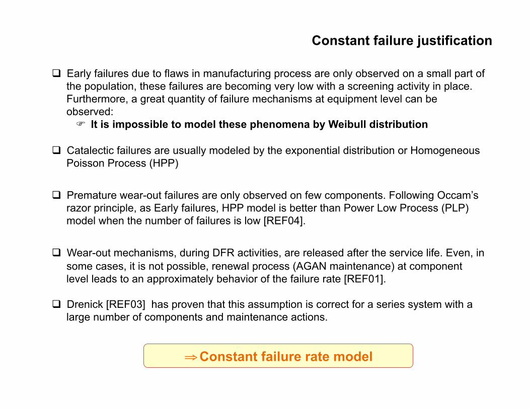
Constant failure justification

q  Early failures due to flaws in manufacturing process are only observed on a small part of the population, these failures are becoming very low with a screening activity in place. Furthermore, a great quantity of failure mechanisms at equipment level can be observed: F  It is impossible to model these phenomena by Weibull distribution

q  Catalectic failures are usually modeled by the exponential distribution or Homogeneous

Poisson Process (HPP)

q  Premature wear-out failures are only observed on few components. Following Occam’s razor principle, as Early failures, HPP model is better than Power Low Process (PLP) model when the number of failures is low [REF04].

q  Wear-out mechanisms, during DFR activities, are released after the service life. Even, in

some cases, it is not possible, renewal process (AGAN maintenance) at component level leads to an approximately behavior of the failure rate [REF01].

q  Drenick [REF03] has proven that this assumption is correct for a series system with a large number of components and maintenance actions.

⇒ Constant failure rate model

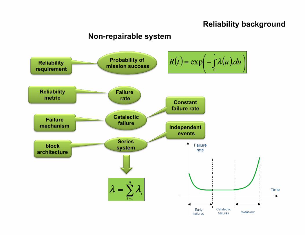
Non-repairable system

Probability of mission success

∑=

=n

ii

1λλ

Reliability requirement

Reliability metric

Failure rate

Failure mechanism

Catalectic failure

( ) ( ) ⎟⎠⎞

⎜⎝⎛−= ∫

t

duutR0

.exp λ

block architecture

Series system

Reliability background

Constant failure rate

Independent events

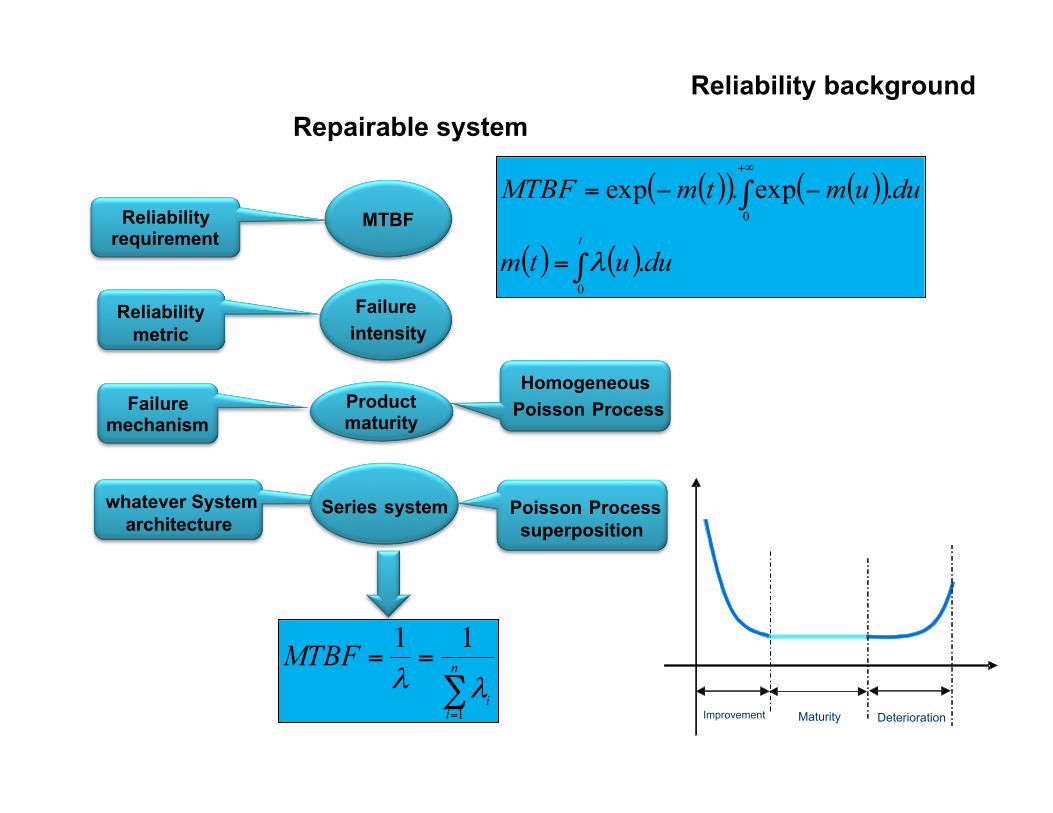
Repairable system

MTBF

∑=

== n

ii

MTBF

1

11

λλ

Reliability requirement

Reliability metric

Failure intensity

Failure mechanism

Product maturity

( )( ) ( )( )

( ) ( )∫

∫

=

−−=+∞

t

duutm

duumtmMTBF

0

0

.

.exp.exp

λ

whatever System architecture

Series system

Reliability background

Homogeneous Poisson Process

Poisson Process superposition

Maturity Deterioration Improvement

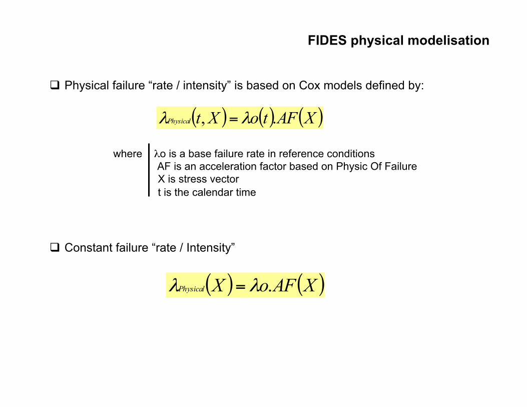
FIDES physical modelisation

q  Physical failure “rate / intensity” is based on Cox models defined by:

( ) ( ) ( )XAFtoXtPhysical ., λλ =

where λo is a base failure rate in reference conditions AF is an acceleration factor based on Physic Of Failure X is stress vector t is the calendar time

q  Constant failure “rate / Intensity”

( ) ( )XAFoXPhysical .λλ =

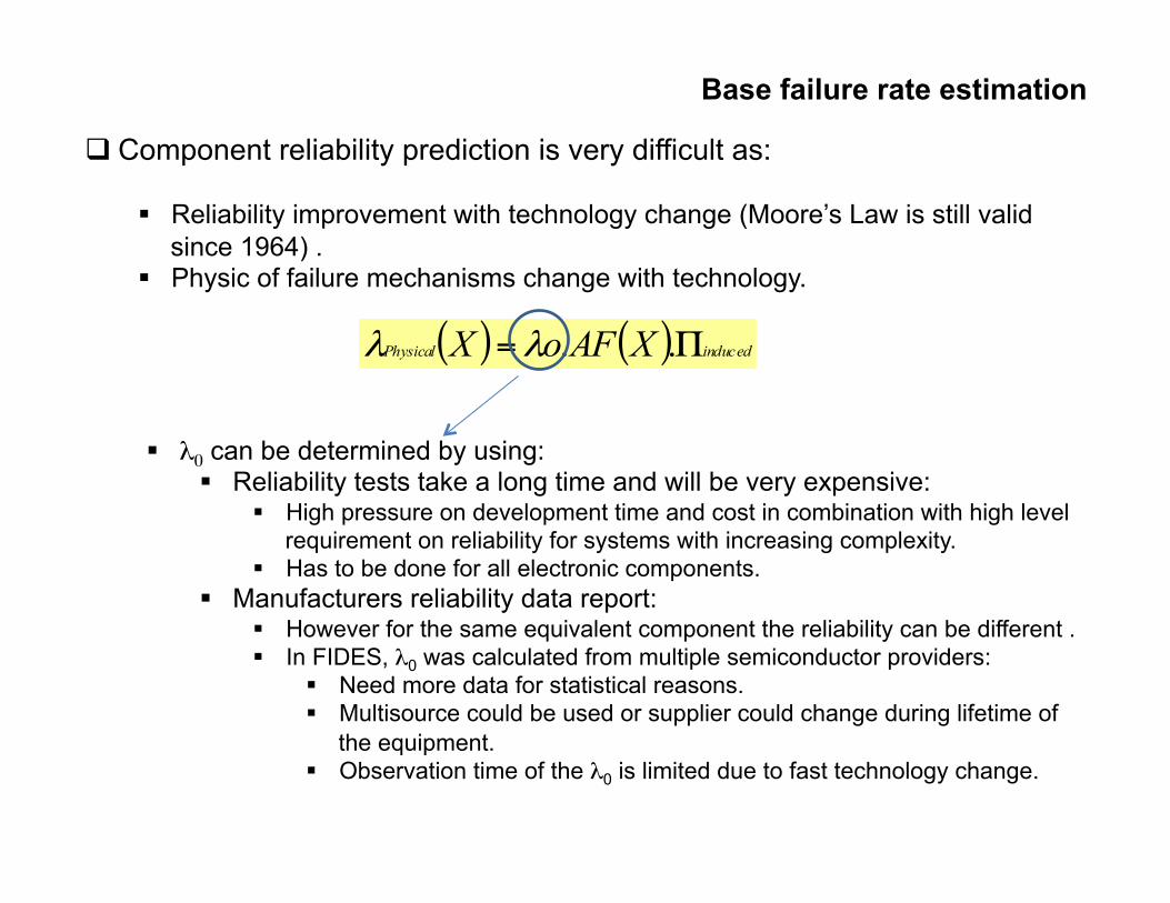
Base failure rate estimation

q Component reliability prediction is very difficult as:

§  Reliability improvement with technology change (Moore’s Law is still valid since 1964) .

§  Physic of failure mechanisms change with technology.

( ) ( ) inducedPhysical XAFoX Π= ..λλ

§  λ0 can be determined by using: §  Reliability tests take a long time and will be very expensive:

§  High pressure on development time and cost in combination with high level requirement on reliability for systems with increasing complexity.

§  Has to be done for all electronic components. §  Manufacturers reliability data report:

§  However for the same equivalent component the reliability can be different . §  In FIDES, λ0 was calculated from multiple semiconductor providers:

§  Need more data for statistical reasons. §  Multisource could be used or supplier could change during lifetime of

the equipment. §  Observation time of the λ0 is limited due to fast technology change.

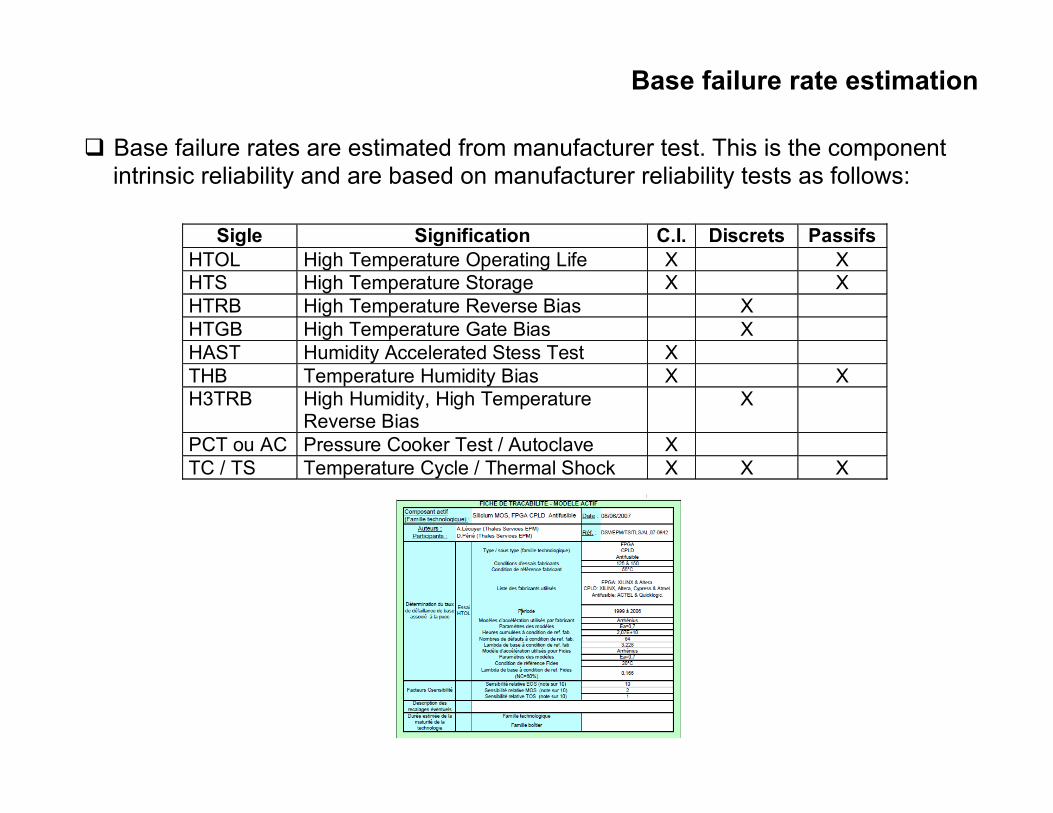
Base failure rate estimation

q  Base failure rates are estimated from manufacturer test. This is the component intrinsic reliability and are based on manufacturer reliability tests as follows:

Sigle Signification C.I. Discrets PassifsHTOL High Temperature Operating Life X XHTS High Temperature Storage X XHTRB High Temperature Reverse Bias XHTGB High Temperature Gate Bias XHAST Humidity Accelerated Stess Test XTHB Temperature Humidity Bias X XH3TRB High Humidity, High Temperature

Reverse BiasX

PCT ou AC Pressure Cooker Test / Autoclave XTC / TS Temperature Cycle / Thermal Shock X X X

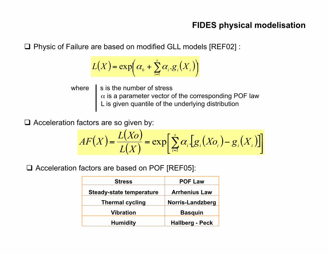
FIDES physical modelisation

q  Physic of Failure are based on modified GLL models [REF02] :

( ) ( )⎟⎠⎞⎜

⎝⎛ += ∑

=

s

iiii XgXL

10 .exp αα

where s is the number of stress α is a parameter vector of the corresponding POF law L is given quantile of the underlying distribution

q  Acceleration factors are so given by:

( ) ( )( )

( ) ( )[ ]⎥⎦⎤

⎢⎣⎡ −== ∑

=

s

iiiiii XgXog

XLXoLXAF

1.exp α

q  Acceleration factors are based on POF [REF05]:

Stress POF Law

Steady-state temperature Arrhenius Law

Thermal cycling Norris-Landzberg

Vibration Basquin

Humidity Hallberg - Peck

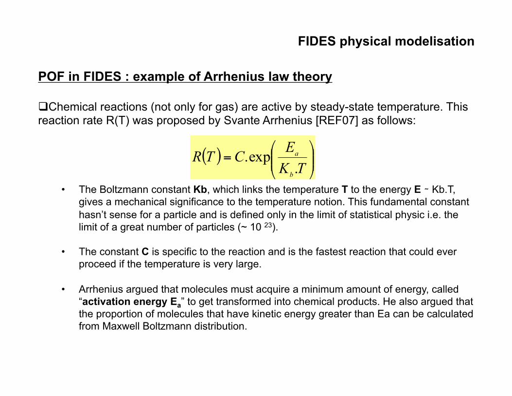
FIDES physical modelisation

POF in FIDES : example of Arrhenius law theory q Chemical reactions (not only for gas) are active by steady-state temperature. This reaction rate R(T) was proposed by Svante Arrhenius [REF07] as follows:

•  The Boltzmann constant Kb, which links the temperature T to the energy E ∼ Kb.T, gives a mechanical significance to the temperature notion. This fundamental constant hasn’t sense for a particle and is defined only in the limit of statistical physic i.e. the limit of a great number of particles (~ 10 23).

•  The constant C is specific to the reaction and is the fastest reaction that could ever proceed if the temperature is very large.

•  Arrhenius argued that molecules must acquire a minimum amount of energy, called “activation energy Ea” to get transformed into chemical products. He also argued that the proportion of molecules that have kinetic energy greater than Ea can be calculated from Maxwell Boltzmann distribution.

( ) ⎟⎟⎠

⎞⎜⎜⎝

⎛=

TKECTRb

a

.exp.

FIDES physical modelisation

High activation energy

Low activation energy

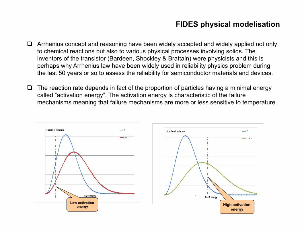
q  Arrhenius concept and reasoning have been widely accepted and widely applied not only to chemical reactions but also to various physical processes involving solids. The inventors of the transistor (Bardeen, Shockley & Brattain) were physicists and this is perhaps why Arrhenius law have been widely used in reliability physics problem during the last 50 years or so to assess the reliability for semiconductor materials and devices.

q  The reaction rate depends in fact of the proportion of particles having a minimal energy called “activation energy”. The activation energy is characteristic of the failure mechanisms meaning that failure mechanisms are more or less sensitive to temperature

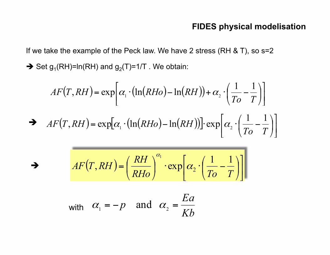
If we take the example of the Peck law. We have 2 stress (RH & T), so s=2 è Set g1(RH)=ln(RH) and g2(T)=1/T . We obtain:

( ) ( ) ( )( ) ⎥⎦

⎤⎢⎣

⎡⎟⎠

⎞⎜⎝

⎛ −⋅+−⋅=TTo

RHRHoRHTAF 11lnlnexp, 21 αα

è ( ) ( ) ( )( )[ ] ⎥⎦

⎤⎢⎣

⎡⎟⎠

⎞⎜⎝

⎛ −⋅⋅−⋅=TTo

RHRHoRHTAF 11explnlnexp, 21 αα

è ( ) ⎥⎦

⎤⎢⎣

⎡⎟⎠

⎞⎜⎝

⎛ −⋅⋅⎟⎠

⎞⎜⎝

⎛=TToRHo

RHRHTAF 11exp, 2

1

αα

with KbEap =−= 21 and αα

FIDES physical modelisation

Acceleration factor estimation

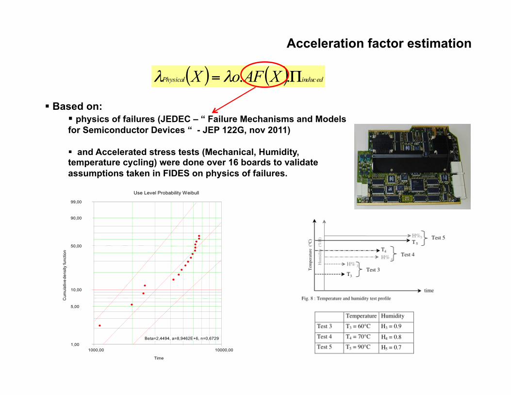
§  Based on: §  physics of failures (JEDEC – “ Failure Mechanisms and Models for Semiconductor Devices “ - JEP 122G, nov 2011)

§  and Accelerated stress tests (Mechanical, Humidity, temperature cycling) were done over 16 boards to validate assumptions taken in FIDES on physics of failures.

( ) ( ) inducedPhysical XAFoX Π= ..λλ

1,00

5,00

10,00

50,00

90,00

99,00

1000,00 10000,00

Use Level Probability Weibull

Time

Cum

ulat

ive d

ensi

ty fu

nctio

n

Beta=2,4494, a=8,9462E+6, n=0,6729

Integrated Circuit Acceleration factor for Thermal Stress

( )⎥⎥⎦

⎤

⎢⎢⎣

⎡

+−××

− 273T1

29310.711604

componentje

Reciprocal of the Boltzmann’s constant.

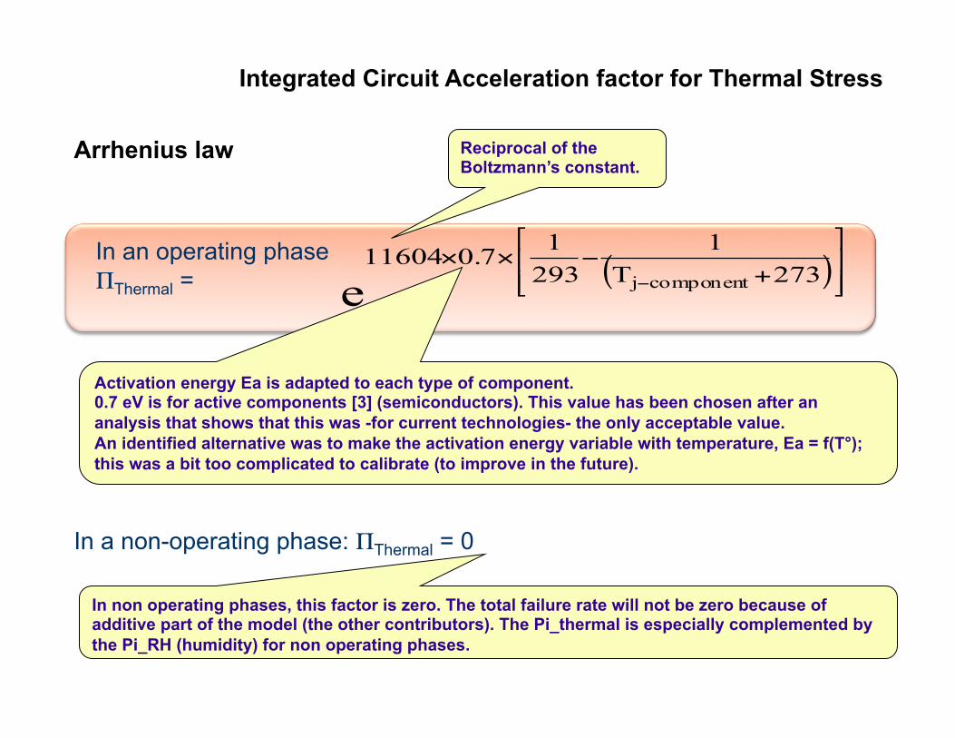
Activation energy Ea is adapted to each type of component. 0.7 eV is for active components [3] (semiconductors). This value has been chosen after an analysis that shows that this was -for current technologies- the only acceptable value. An identified alternative was to make the activation energy variable with temperature, Ea = f(T°); this was a bit too complicated to calibrate (to improve in the future).

Arrhenius law

In an operating phase ΠThermal =

In a non-operating phase: ΠThermal = 0

In non operating phases, this factor is zero. The total failure rate will not be zero because of additive part of the model (the other contributors). The Pi_thermal is especially complemented by the Pi_RH (humidity) for non operating phases.

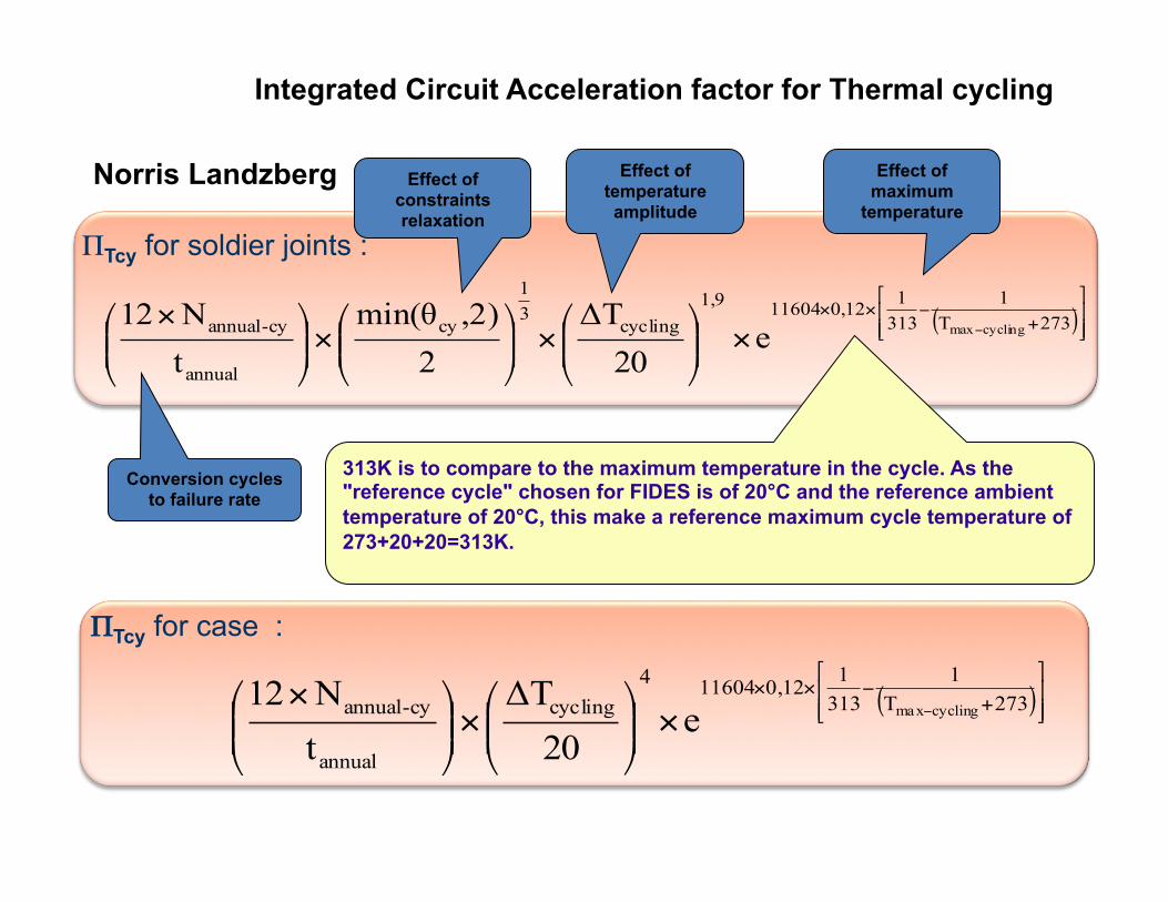
Integrated Circuit Acceleration factor for Thermal cycling

( )⎥⎥⎦

⎤

⎢⎢⎣

⎡

+−××

−×⎟⎟⎠

⎞⎜⎜⎝

⎛×⎟⎟

⎠

⎞⎜⎜⎝

⎛×⎟⎟⎠

⎞⎜⎜⎝

⎛ × 273T1

31310,12116041,9

cycling31

cy

annual

cy-annual cyclingmaxe20

ΔT2,2)min(θ

tN12

( )⎥⎥⎦

⎤

⎢⎢⎣

⎡

+−××

−×⎟⎟⎠

⎞⎜⎜⎝

⎛×⎟⎟⎠

⎞⎜⎜⎝

⎛ × 273T1

313112,0116044

cycling

annual

cy-annual cyclingmaxe20

ΔTtN12

Norris Landzberg

ΠTcy for soldier joints :

313K is to compare to the maximum temperature in the cycle. As the "reference cycle" chosen for FIDES is of 20°C and the reference ambient temperature of 20°C, this make a reference maximum cycle temperature of 273+20+20=313K.

Effect of temperature amplitude

Effect of maximum

temperature

Effect of constraints relaxation

Conversion cycles to failure rate

ΠTcy for case :

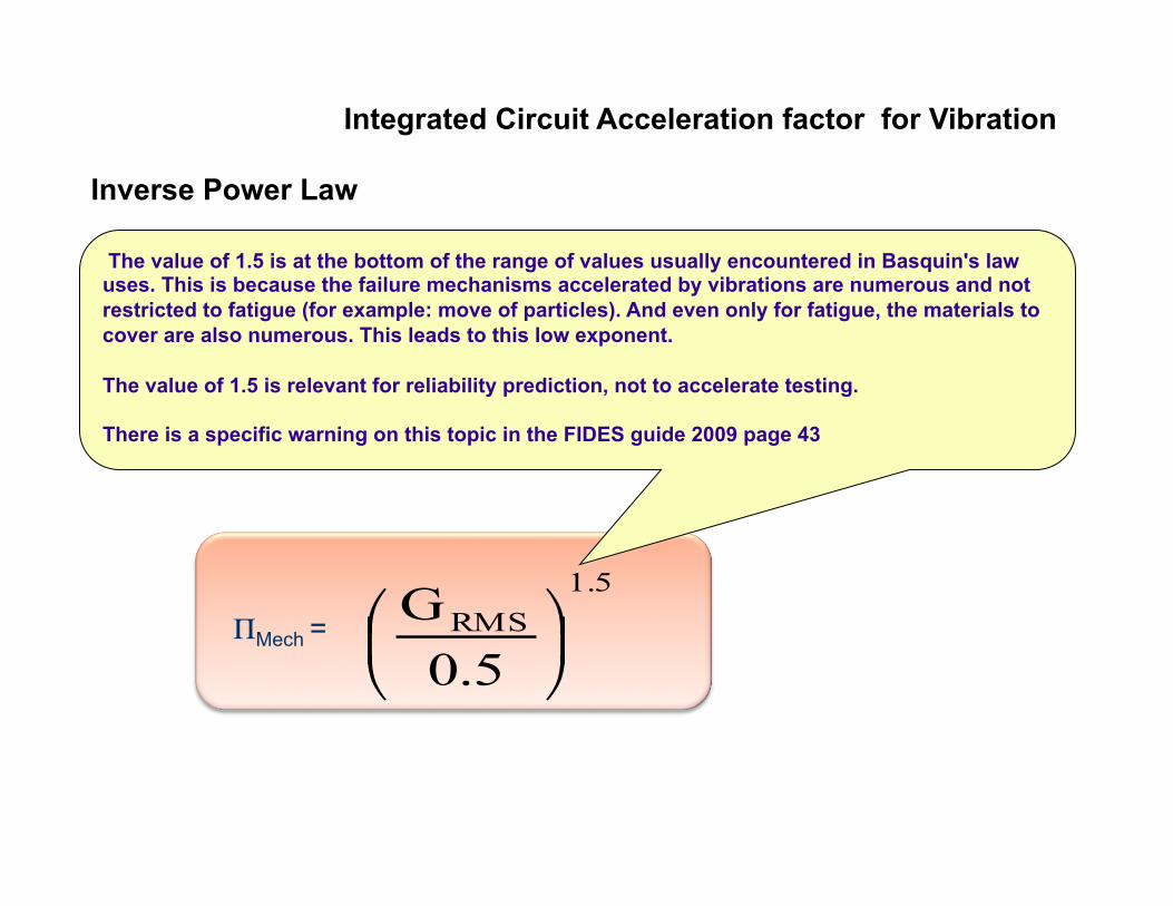
Integrated Circuit Acceleration factor for Vibration

1.5RMS

0.5G

⎟⎠

⎞⎜⎝

⎛

The value of 1.5 is at the bottom of the range of values usually encountered in Basquin's law uses. This is because the failure mechanisms accelerated by vibrations are numerous and not restricted to fatigue (for example: move of particles). And even only for fatigue, the materials to cover are also numerous. This leads to this low exponent. The value of 1.5 is relevant for reliability prediction, not to accelerate testing. There is a specific warning on this topic in the FIDES guide 2009 page 43

Inverse Power Law

ΠMech =

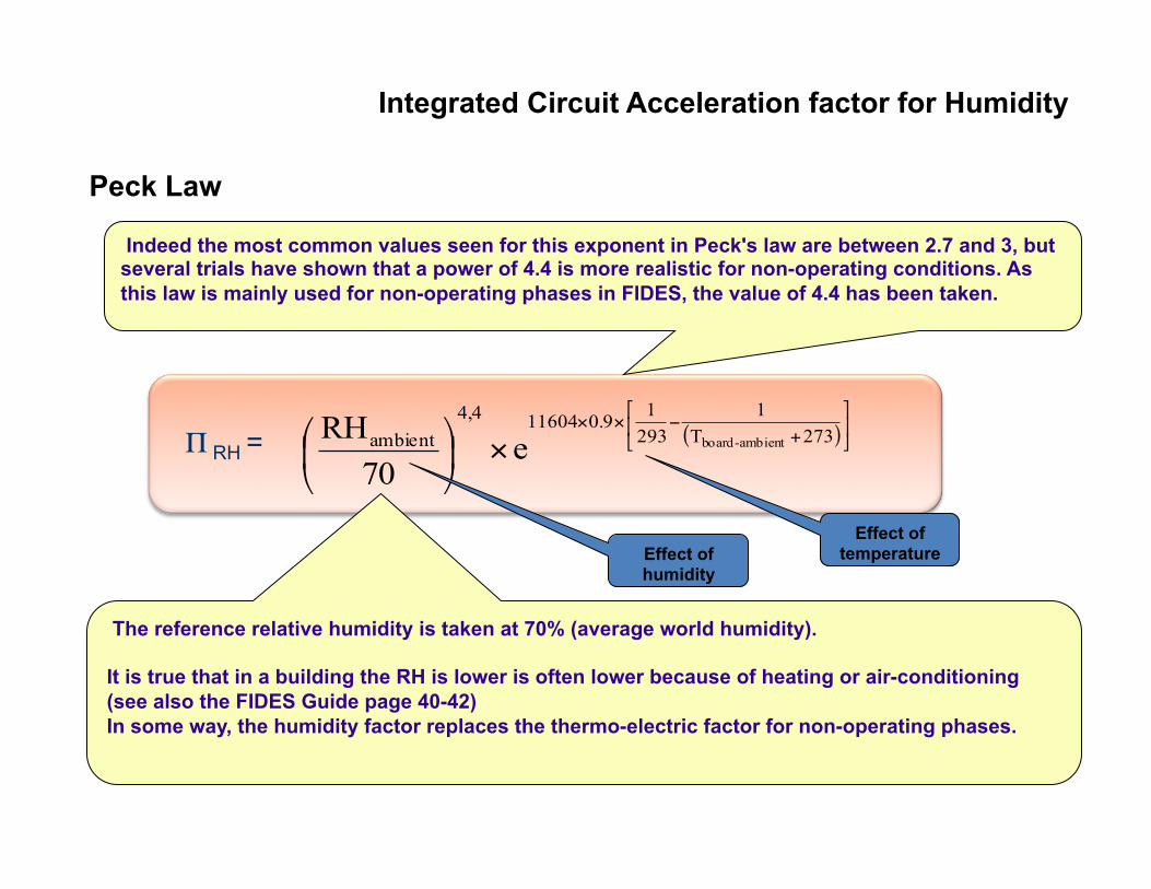
Integrated Circuit Acceleration factor for Humidity

Peck Law

Π RH = ( )⎥⎦⎤

⎢⎣

⎡

+−××

×⎟⎠

⎞⎜⎝

⎛ 273T1

29310.9116044,4

ambient ambient-boarde70

RH

Indeed the most common values seen for this exponent in Peck's law are between 2.7 and 3, but several trials have shown that a power of 4.4 is more realistic for non-operating conditions. As this law is mainly used for non-operating phases in FIDES, the value of 4.4 has been taken.

.

The reference relative humidity is taken at 70% (average world humidity). It is true that in a building the RH is lower is often lower because of heating or air-conditioning (see also the FIDES Guide page 40-42) In some way, the humidity factor replaces the thermo-electric factor for non-operating phases.

Effect of temperature Effect of

humidity

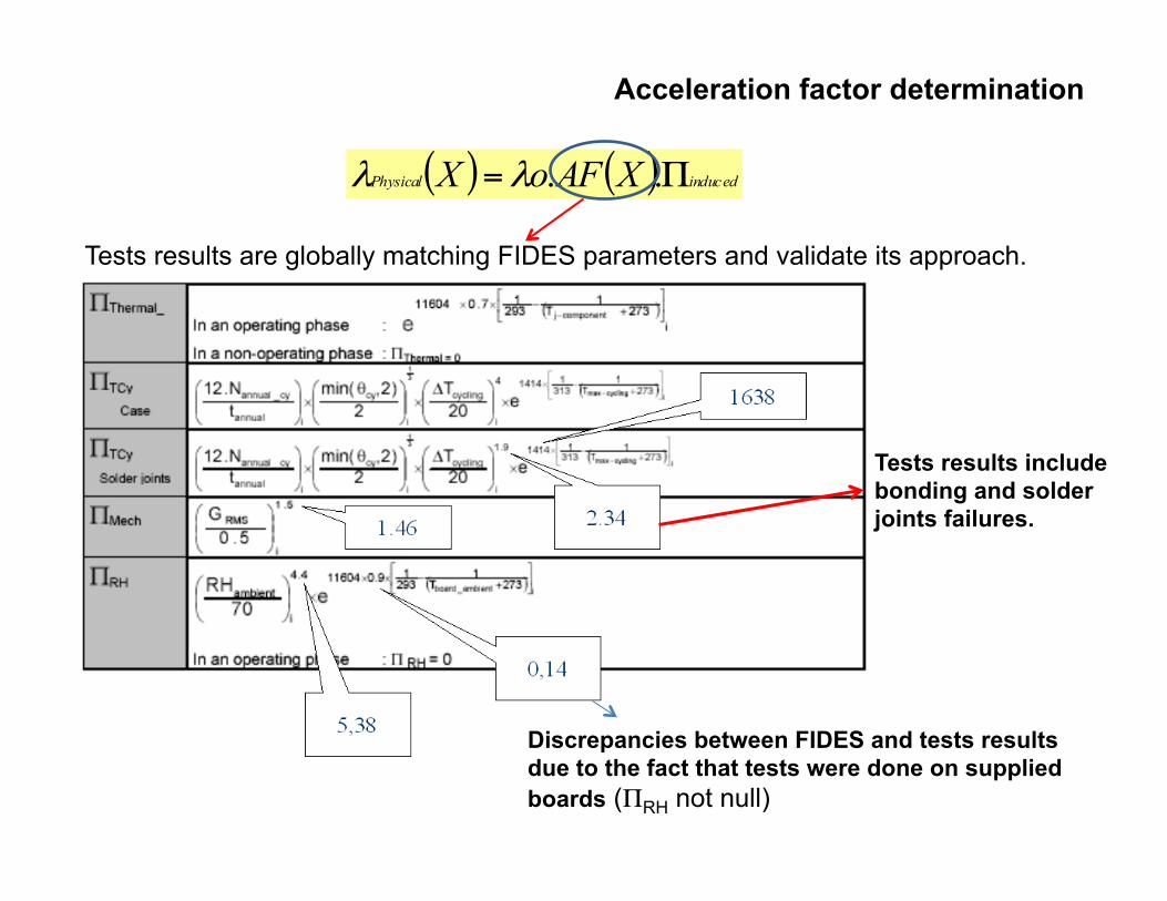
Acceleration factor determination

( ) ( ) inducedPhysical XAFoX Π= ..λλ

Discrepancies between FIDES and tests results due to the fact that tests were done on supplied boards (ΠRH not null)

Tests results include bonding and solder joints failures.

Tests results are globally matching FIDES parameters and validate its approach.

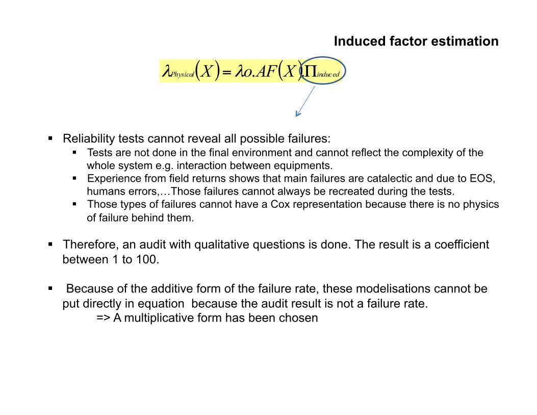
Induced factor estimation

§  Reliability tests cannot reveal all possible failures:

§  Tests are not done in the final environment and cannot reflect the complexity of the whole system e.g. interaction between equipments.

§  Experience from field returns shows that main failures are catalectic and due to EOS, humans errors,…Those failures cannot always be recreated during the tests.

§  Those types of failures cannot have a Cox representation because there is no physics of failure behind them.

§  Therefore, an audit with qualitative questions is done. The result is a coefficient between 1 to 100.

§  Because of the additive form of the failure rate, these modelisations cannot be put directly in equation because the audit result is not a failure rate.

=> A multiplicative form has been chosen

( ) ( ) inducedPhysical XAFoX Π= ..λλ

TERMINOLOGY

AGAN : As Good As New COTS : Component On The Shelf DFR : Design For Reliability GLL : General Log Linear HASS : Highly Accelerated Step Stress HAT : Highly Accelerated Test HPP : Homogeneous Poisson Process MTBF : Mean Time Between Failure PLP : Power Law Process

Document reference

[REF01] : “Statistical Methods for the reliability of repairable systems” Steven E.RIGDON & Asit P.BASU Wiley 2000

[REF02] : “Modeling & Analysis for Multiple Stress-Type Accelerated Life Data

Adamantios METTAS 2000 PROCEEDINGS Annual RELIABILITY and MAINTAINABILITY Symposium [REF03] : « The failure law of complex equipment »

R.F.DRENICK J.Soc.Indust.Appl.Math.1960 Vol 8 N°4 [REF04] : “ The effect of assuming a HPP when the true process is a PLP”

Steven E.RIGDON & Asit P.BASU Journal of Quality technology 1990 [REF05] : JEDEC Standards

JEP122G [REF06] : FIDES Guide 2009 [REF07] : «Über die Reaktion-geschwindigkeit bei der Inversion vor Rhorzücker durch Sauren “

S.ARRHENIUS Z. Phys.-Ch., 1889.