1-5: Least-squaresI - 國立臺灣大學cjlin/courses/optml2018/notes.pdf1-5: Least-squaresII...
228
1-5: Least-squares I A:k n. Usually k>n otherwise easily the minimum is zero. Analytical solution: f (x) =( Ax b) T (Ax b) =x T A T Ax 2b T Ax + b T b r f (x) = 2 A T Ax 2A T b=0 Chih-Jen Lin (National Taiwan Univ.) Optimization and Machine Learning 1 / 228
Transcript of 1-5: Least-squaresI - 國立臺灣大學cjlin/courses/optml2018/notes.pdf1-5: Least-squaresII...
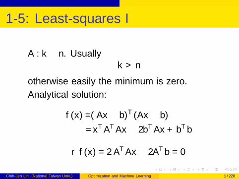
1-5: Least-squares I
A : k × n. Usuallyk > n
otherwise easily the minimum is zero.
Analytical solution:
f (x) =(Ax − b)T (Ax − b)
=xTATAx − 2bTAx + bTb
∇f (x) = 2ATAx − 2ATb = 0
Chih-Jen Lin (National Taiwan Univ.) Optimization and Machine Learning 1 / 228
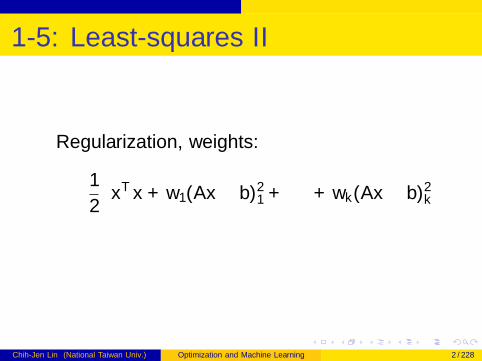
1-5: Least-squares II
Regularization, weights:
1
2λxTx + w1(Ax − b)2
1 + · · ·+ wk(Ax − b)2k
Chih-Jen Lin (National Taiwan Univ.) Optimization and Machine Learning 2 / 228
2-4: Convex Combination and ConvexHull I
Convex hull is convex
x = θ1x1 + · · ·+ θkxk
x = θ1x1 + · · ·+ θk xk
Then
αx + (1− α)x
=αθ1x1 + · · ·+ αθkxk+
(1− α)θ1x1 + · · ·+ (1− α)θk xk
Chih-Jen Lin (National Taiwan Univ.) Optimization and Machine Learning 3 / 228
2-4: Convex Combination and ConvexHull II
Each coefficient is nonnegative and
αθ1 + · · ·+ αθk + (1− α)θ1 + · · ·+ (1− α)θk= α + (1− α) = 1
Chih-Jen Lin (National Taiwan Univ.) Optimization and Machine Learning 4 / 228
2-7: Euclidean Balls and Ellipsoid I
We prove that any
x = xc + Au with ‖u‖2 ≤ 1
satisfies(x − xc)TP−1(x − xc) ≤ 1
LetA = P1/2
because P is symmetric positive definite.Then
uTATP−1Au = uTP1/2P−1P1/2u ≤ 1.
Chih-Jen Lin (National Taiwan Univ.) Optimization and Machine Learning 5 / 228
2-10: Positive Semidefinite Cone I
Sn+ is a convex cone. Let
X1,X2 ∈ Sn+
For any θ1 ≥ 0, θ2 ≥ 0,
zT (θ1X1 + θ2X2)z = θ1zTX1z + θ2z
TX2z ≥ 0
Chih-Jen Lin (National Taiwan Univ.) Optimization and Machine Learning 6 / 228
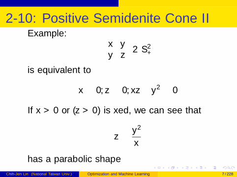
2-10: Positive Semidefinite Cone IIExample: [
x yy z
]∈ S2
+
is equivalent to
x ≥ 0, z ≥ 0, xz − y 2 ≥ 0
If x > 0 or (z > 0) is fixed, we can see that
z ≥ y 2
x
has a parabolic shape
Chih-Jen Lin (National Taiwan Univ.) Optimization and Machine Learning 7 / 228
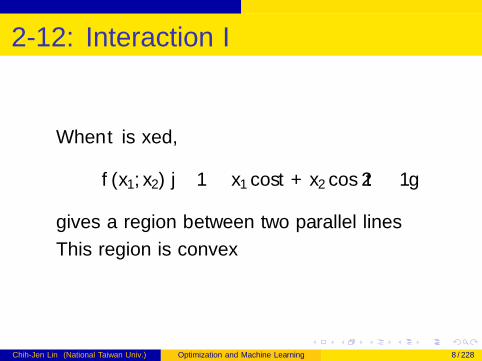
2-12: Interaction I
When t is fixed,
{(x1, x2) | −1 ≤ x1 cos t + x2 cos 2t ≤ 1}
gives a region between two parallel lines
This region is convex
Chih-Jen Lin (National Taiwan Univ.) Optimization and Machine Learning 8 / 228
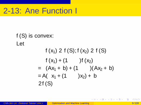
2-13: Affine Function I
f (S) is convex:
Letf (x1) ∈ f (S), f (x2) ∈ f (S)
αf (x1) + (1− α)f (x2)
=α(Ax1 + b) + (1− α)(Ax2 + b)
=A(αx1 + (1− α)x2) + b
∈f (S)
Chih-Jen Lin (National Taiwan Univ.) Optimization and Machine Learning 9 / 228
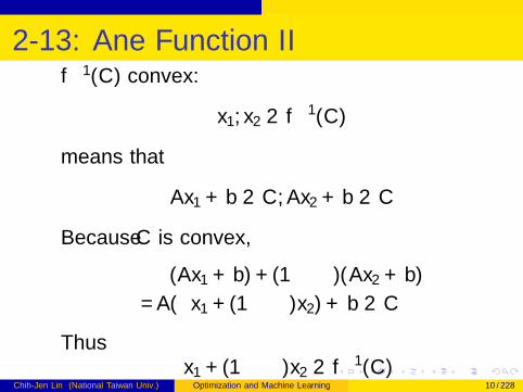
2-13: Affine Function IIf −1(C ) convex:
x1, x2 ∈ f −1(C )
means that
Ax1 + b ∈ C ,Ax2 + b ∈ C
Because C is convex,
α(Ax1 + b) + (1− α)(Ax2 + b)
=A(αx1 + (1− α)x2) + b ∈ C
Thusαx1 + (1− α)x2 ∈ f −1(C )
Chih-Jen Lin (National Taiwan Univ.) Optimization and Machine Learning 10 / 228
2-13: Affine Function III
Scaling:αS = {αx | x ∈ S}
Translation
S + a = {x + a | x ∈ S}
Projection
T = {x1 ∈ Rm | (x1, x2) ∈ S , x2 ∈ Rn}, S ⊆ Rm×Rn
Scaling, translation, and projection are all affinefunctions
Chih-Jen Lin (National Taiwan Univ.) Optimization and Machine Learning 11 / 228
2-13: Affine Function IV
For example, for projection
f (x) =[I 0
] [x1
x2
]+ 0
I : identity matrix
Solution set of linear matrix inequality
C = {S | S � 0} is convex
f (x) = x1A1 + · · ·+ xmAm − B = Ax + b
f −1(C ) = {x | f (x) � 0} is convex
Chih-Jen Lin (National Taiwan Univ.) Optimization and Machine Learning 12 / 228
2-13: Affine Function V
But this isn’t rigourous because of some problems inarguing
f (x) = Ax + b
A more formal explanation:
C = {s ∈ Rp2 | mat(s) ∈ Sp and mat(s) � 0}
is convex
f (x) = x1vec(A1) + · · ·+ xmvec(Am)− vec(B)
=[vec(A1) · · · vec(Am)
]x + (−vec(B))
Chih-Jen Lin (National Taiwan Univ.) Optimization and Machine Learning 13 / 228
2-13: Affine Function VI
f −1(C ) = {x | mat(f (x)) ∈ Sp and mat(f (x)) � 0}
is convex
Hyperbolic cone:
C = {(z , t) | zT z ≤ t2, t ≥ 0}
is convex (by drawing a figure in 2 or 3 dimensionalspace)
Chih-Jen Lin (National Taiwan Univ.) Optimization and Machine Learning 14 / 228
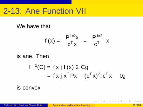
2-13: Affine Function VII
We have that
f (x) =
[P1/2xcTx
]=
[P1/2
cT
]x
is affine. Then
f −1(C ) = {x | f (x) ∈ C}= {x | xTPx ≤ (cTx)2, cTx ≥ 0}
is convex
Chih-Jen Lin (National Taiwan Univ.) Optimization and Machine Learning 15 / 228
Perspective and linear-fractional function I
Image convex: if S is convex, check if
{P(x , t) | (x , t) ∈ S}
convex or not
Note that S is in the domain of P
Chih-Jen Lin (National Taiwan Univ.) Optimization and Machine Learning 16 / 228
Perspective and linear-fractional functionII
Assume(x1, t1), (x2, t2) ∈ S
We hope
αx1
t1+ (1− α)
x2
t2= P(A,B),
where(A,B) ∈ S
Chih-Jen Lin (National Taiwan Univ.) Optimization and Machine Learning 17 / 228
Perspective and linear-fractional functionIII
We have
αx1
t1+ (1− α)
x2
t2=αt2x1 + (1− α)t1x2
t1t2
=αt2x1 + (1− α)t1x2
αt1t2 + (1− α)t1t2
=
αt2αt2+(1−α)t1
x1 + (1−α)t1αt2+(1−α)t1
x2
αt2αt2+(1−α)t1
t1 + (1−α)t1αt2+(1−α)t1
t2
Chih-Jen Lin (National Taiwan Univ.) Optimization and Machine Learning 18 / 228
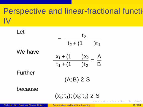
Perspective and linear-fractional functionIV
Let
θ =αt2
αt2 + (1− α)t1
We haveθx1 + (1− θ)x2
θt1 + (1− θ)t2=
A
B
Further(A,B) ∈ S
because(x1, t1), (x2, t2) ∈ S
Chih-Jen Lin (National Taiwan Univ.) Optimization and Machine Learning 19 / 228
Perspective and linear-fractional functionV
andS is convex
Inverse image is convex
Given C a convex set
P−1(C ) = {(x , t) | P(x , t) = x/t ∈ C}
is convex
Chih-Jen Lin (National Taiwan Univ.) Optimization and Machine Learning 20 / 228
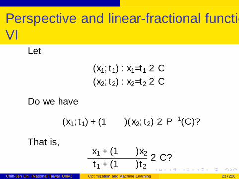
Perspective and linear-fractional functionVI
Let
(x1, t1) : x1/t1 ∈ C
(x2, t2) : x2/t2 ∈ C
Do we have
θ(x1, t1) + (1− θ)(x2, t2) ∈ P−1(C )?
That is,θx1 + (1− θ)x2
θt1 + (1− θ)t2∈ C?
Chih-Jen Lin (National Taiwan Univ.) Optimization and Machine Learning 21 / 228
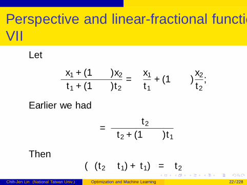
Perspective and linear-fractional functionVII
Let
θx1 + (1− θ)x2
θt1 + (1− θ)t2= α
x1
t1+ (1− α)
x2
t2,
Earlier we had
θ =αt2
αt2 + (1− α)t1
Then(α(t2 − t1) + t1)θ = αt2
Chih-Jen Lin (National Taiwan Univ.) Optimization and Machine Learning 22 / 228
Perspective and linear-fractional functionVIII
t1θ = αt2 − αt2θ + αt1θ
α =t1θ
t1θ + (1− θ)t2
Chih-Jen Lin (National Taiwan Univ.) Optimization and Machine Learning 23 / 228
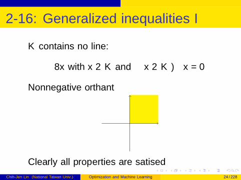
2-16: Generalized inequalities I
K contains no line:
∀x with x ∈ K and − x ∈ K ⇒ x = 0
Nonnegative orthant
Clearly all properties are satisfied
Chih-Jen Lin (National Taiwan Univ.) Optimization and Machine Learning 24 / 228
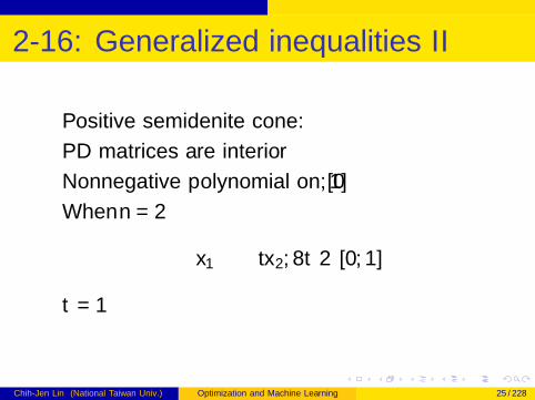
2-16: Generalized inequalities II
Positive semidefinite cone:
PD matrices are interior
Nonnegative polynomial on [0, 1]
When n = 2
x1 ≥ −tx2,∀t ∈ [0, 1]
t = 1
Chih-Jen Lin (National Taiwan Univ.) Optimization and Machine Learning 25 / 228
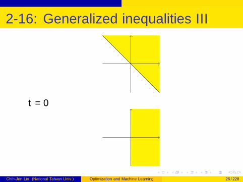
2-16: Generalized inequalities III
t = 0
Chih-Jen Lin (National Taiwan Univ.) Optimization and Machine Learning 26 / 228
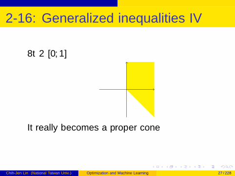
2-16: Generalized inequalities IV
∀t ∈ [0, 1]
It really becomes a proper cone
Chih-Jen Lin (National Taiwan Univ.) Optimization and Machine Learning 27 / 228
2-17: I
Properties:x �K y , u �K v
implies that
y − x ∈ K
v − u ∈ K
From the definition of a convex cone,
(y − x) + (v − u) ∈ K
Thenx + u �K y + v
Chih-Jen Lin (National Taiwan Univ.) Optimization and Machine Learning 28 / 228
2-18: Minimum and minimal elements I
The minimum element
S ⊆ x1 + K
A minimal element
(x2 − K ) ∩ S = {x2}
Chih-Jen Lin (National Taiwan Univ.) Optimization and Machine Learning 29 / 228
2-19: Separating hyperplane theorem I
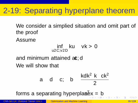
We consider a simplified situation and omit part ofthe proof
Assumeinf
u∈C ,v∈D‖u − v‖ > 0
and minimum attained at c , d
We will show that
a ≡ d − c , b ≡ ‖d‖2 − ‖c‖2
2
forms a separating hyperplane aTx = bChih-Jen Lin (National Taiwan Univ.) Optimization and Machine Learning 30 / 228
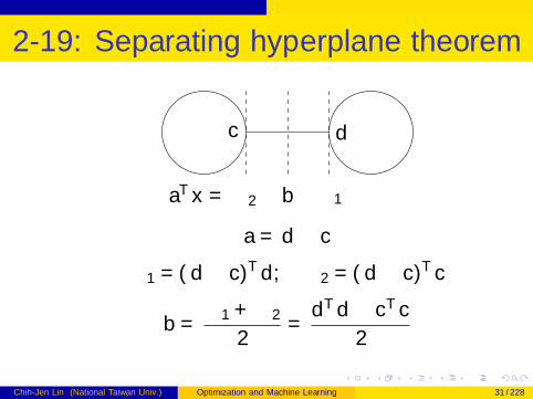
2-19: Separating hyperplane theorem II
aTx = ∆2 b ∆1
c d
a = d − c
∆1 = (d − c)Td , ∆2 = (d − c)Tc
b =∆1 + ∆2
2=
dTd − cTc
2
Chih-Jen Lin (National Taiwan Univ.) Optimization and Machine Learning 31 / 228
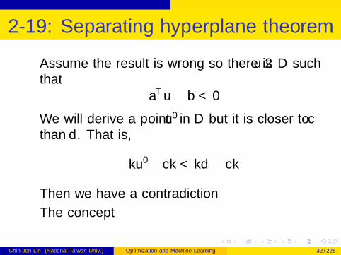
2-19: Separating hyperplane theorem III
Assume the result is wrong so there is u ∈ D suchthat
aTu − b < 0
We will derive a point u′ in D but it is closer to cthan d . That is,
‖u′ − c‖ < ‖d − c‖
Then we have a contradiction
The concept
Chih-Jen Lin (National Taiwan Univ.) Optimization and Machine Learning 32 / 228
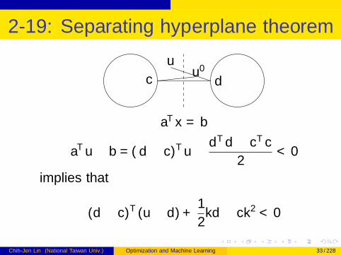
2-19: Separating hyperplane theorem IV
aTx = b
c d
uu′
aTu − b = (d − c)Tu − dTd − cTc
2< 0
implies that
(d − c)T (u − d) +1
2‖d − c‖2 < 0
Chih-Jen Lin (National Taiwan Univ.) Optimization and Machine Learning 33 / 228
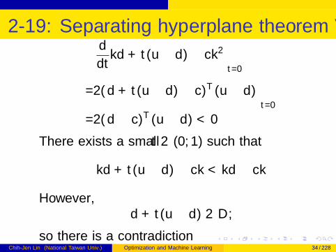
2-19: Separating hyperplane theorem Vd
dt‖d + t(u − d)− c‖2
∣∣∣∣t=0
=2(d + t(u − d)− c)T (u − d)
∣∣∣∣t=0
=2(d − c)T (u − d) < 0
There exists a small t ∈ (0, 1) such that
‖d + t(u − d)− c‖ < ‖d − c‖
However,d + t(u − d) ∈ D,
so there is a contradictionChih-Jen Lin (National Taiwan Univ.) Optimization and Machine Learning 34 / 228
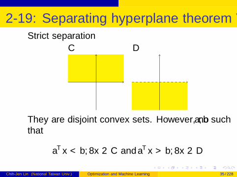
2-19: Separating hyperplane theorem VIStrict separation
C D
They are disjoint convex sets. However, no a, b suchthat
aTx < b,∀x ∈ C and aTx > b,∀x ∈ D
Chih-Jen Lin (National Taiwan Univ.) Optimization and Machine Learning 35 / 228
2-20: Supporting hyperplane theorem I
Case 1: C has an interior region
Consider 2 sets:
interior of C versus {x0},where x0 is any boundary point
If C is convex, then interior of C is also convex
Then both sets are convex
We can apply results in slide 2-19 so that thereexists a such that
aTx ≤ aTx0,∀x ∈ interior of C
Chih-Jen Lin (National Taiwan Univ.) Optimization and Machine Learning 36 / 228
2-20: Supporting hyperplane theorem II
Then for all boundary point x we also have
aTx ≤ aTx0
because any boundary point is the limit of interiorpoints
Case 2: C has no interior region
In this situation, C is like a line in R3 (so nointerior). Then of course it has a supportinghyperplane
We don’t do a rigourous proof here
Chih-Jen Lin (National Taiwan Univ.) Optimization and Machine Learning 37 / 228
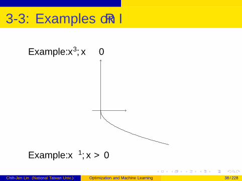
3-3: Examples on R I
Example: x3, x ≥ 0
Example: x−1, x > 0
Chih-Jen Lin (National Taiwan Univ.) Optimization and Machine Learning 38 / 228
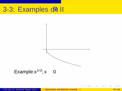
3-3: Examples on R II
Example: x1/2, x ≥ 0
Chih-Jen Lin (National Taiwan Univ.) Optimization and Machine Learning 39 / 228
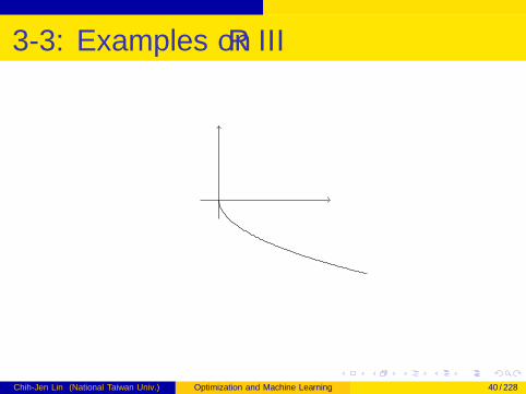
3-3: Examples on R III
Chih-Jen Lin (National Taiwan Univ.) Optimization and Machine Learning 40 / 228
3-4: Examples on Rn and Rm×n I
A,X ∈ Rm×n
tr(ATX ) =∑j
(ATX )jj
=∑j
∑i
ATji Xij =
∑j
∑i
AijXij
Chih-Jen Lin (National Taiwan Univ.) Optimization and Machine Learning 41 / 228
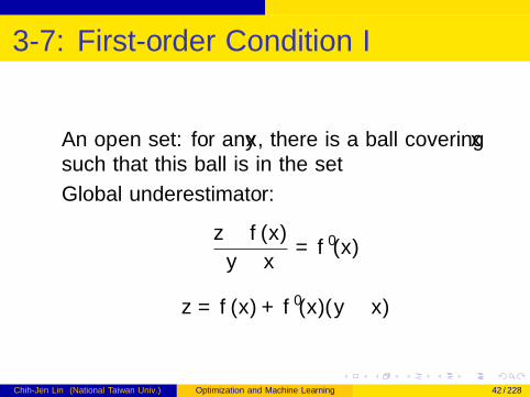
3-7: First-order Condition I
An open set: for any x , there is a ball covering xsuch that this ball is in the set
Global underestimator:
z − f (x)
y − x= f ′(x)
z = f (x) + f ′(x)(y − x)
Chih-Jen Lin (National Taiwan Univ.) Optimization and Machine Learning 42 / 228
3-7: First-order Condition II
⇒: Because domain f is convex,
for all 0 < t ≤ 1, x + t(y − x) ∈ domain f
f (x + t(y − x)) ≤ (1− t)f (x) + tf (y)
f (y) ≥ f (x) +f (x + t(y − x))− f (x)
t
when t → 0,
f (y) ≥ f (x) +∇f (x)T (y − x)
⇐:
Chih-Jen Lin (National Taiwan Univ.) Optimization and Machine Learning 43 / 228
3-7: First-order Condition III
For any 0 ≤ θ ≤ 1,
z = θx + (1− θ)y
f (x) ≥f (z) +∇f (z)T (x − z)
=f (z) +∇f (z)T (1− θ)(x − y)
f (y) ≥f (z) +∇f (z)T (y − z)
=f (z) +∇f (z)Tθ(y − x)
θf (x) + (1− θ)f (y) ≥ f (z)
Chih-Jen Lin (National Taiwan Univ.) Optimization and Machine Learning 44 / 228
3-7: First-order Condition IV
First-order condition for strictly convex function:
f is strictly convex if and only if
f (y) > f (x) +∇f (x)T (y − x)
⇐: it’s easy by directly modifying ≥ to >
f (x) >f (z) +∇f (z)T (x − z)
=f (z) +∇f (z)T (1− θ)(x − y)
f (y) > f (z)+∇f (z)T (y−z) = f (z)+∇f (z)Tθ(y−x)
Chih-Jen Lin (National Taiwan Univ.) Optimization and Machine Learning 45 / 228
3-7: First-order Condition V
⇒: Assume the result is wrong. From the 1st-ordercondition of a convex function, ∃x , y such thatx 6= y and
∇f (x)T (y − x) = f (y)− f (x) (1)
For this (x , y), from the strict convexity
f (x + t(y − x))− f (x) <tf (y)− tf (x)
=∇f (x)T t(y − x),∀t ∈ (0, 1)
Chih-Jen Lin (National Taiwan Univ.) Optimization and Machine Learning 46 / 228
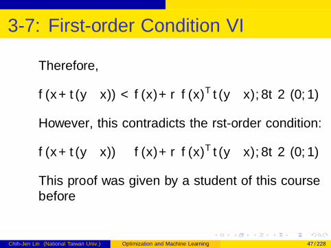
3-7: First-order Condition VI
Therefore,
f (x+t(y−x)) < f (x)+∇f (x)T t(y−x),∀t ∈ (0, 1)
However, this contradicts the first-order condition:
f (x+t(y−x)) ≥ f (x)+∇f (x)T t(y−x),∀t ∈ (0, 1)
This proof was given by a student of this coursebefore
Chih-Jen Lin (National Taiwan Univ.) Optimization and Machine Learning 47 / 228
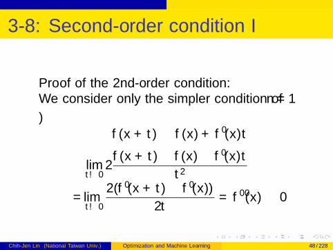
3-8: Second-order condition I
Proof of the 2nd-order condition:We consider only the simpler condition of n = 1
⇒f (x + t) ≥ f (x) + f ′(x)t
limt→0
2f (x + t)− f (x)− f ′(x)t
t2
= limt→0
2(f ′(x + t)− f ′(x))
2t= f ′′(x) ≥ 0
Chih-Jen Lin (National Taiwan Univ.) Optimization and Machine Learning 48 / 228
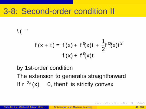
3-8: Second-order condition II
“⇐”
f (x + t) = f (x) + f ′(x)t +1
2f ′′(x)t2
≥ f (x) + f ′(x)t
by 1st-order condition
The extension to general n is straightforward
If ∇2f (x) � 0, then f is strictly convex
Chih-Jen Lin (National Taiwan Univ.) Optimization and Machine Learning 49 / 228
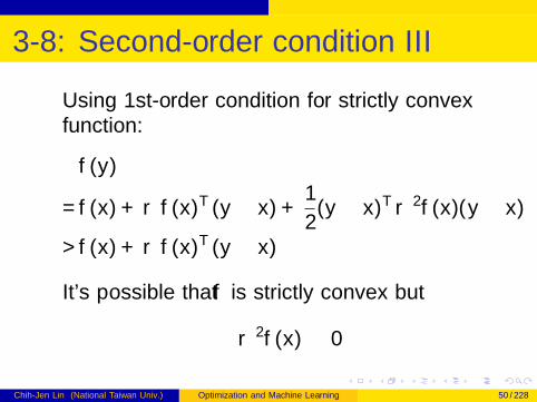
3-8: Second-order condition III
Using 1st-order condition for strictly convexfunction:
f (y)
=f (x) +∇f (x)T (y − x) +1
2(y − x)T∇2f (x)(y − x)
>f (x) +∇f (x)T (y − x)
It’s possible that f is strictly convex but
∇2f (x) � 0
Chih-Jen Lin (National Taiwan Univ.) Optimization and Machine Learning 50 / 228
3-8: Second-order condition IV
Example:
f (x) = x4
Details omitted
Chih-Jen Lin (National Taiwan Univ.) Optimization and Machine Learning 51 / 228
3-9: Examples I
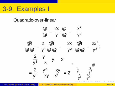
Quadratic-over-linear
∂f
∂x=
2x
y,∂f
∂y= −x
2
y 2
∂2f
∂x∂x=
2
y,∂2f
∂x∂y= −2x
y 2,∂2f
∂y∂y=
2x2
y 3,
2
y 3
[y−x
] [y −x
]=
2
y 3
[y 2 −xy−xy x2
]= 2
[1y − x
y2
− xy2
x2
y3
]Chih-Jen Lin (National Taiwan Univ.) Optimization and Machine Learning 52 / 228
3-10 I
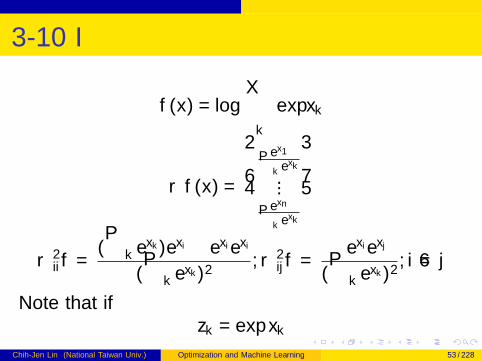
f (x) = log∑k
exp xk
∇f (x) =
ex1∑k e
xk
...exn∑k e
xk
∇2
ii f =(∑
k exk)exi − exiexi
(∑
k exk)2
,∇2ij f =
−exiexj(∑
k exk)2
, i 6= j
Note that ifzk = exp xk
Chih-Jen Lin (National Taiwan Univ.) Optimization and Machine Learning 53 / 228
3-10 II
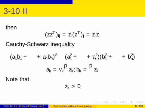
then(zzT )ij = zi(z
T )j = zizj
Cauchy-Schwarz inequality
(a1b1 + · · ·+ anbn)2 ≤ (a21 + · · ·+ a2
n)(b21 + · · ·+ b2
n)
ak = vk√zk , bk =
√zk
Note thatzk > 0
Chih-Jen Lin (National Taiwan Univ.) Optimization and Machine Learning 54 / 228
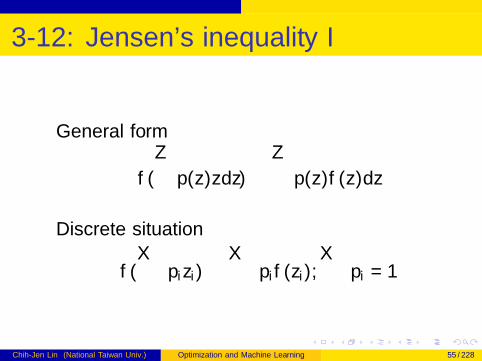
3-12: Jensen’s inequality I
General form
f (
∫p(z)zdz) ≤
∫p(z)f (z)dz
Discrete situation
f (∑
pizi) ≤∑
pi f (zi),∑
pi = 1
Chih-Jen Lin (National Taiwan Univ.) Optimization and Machine Learning 55 / 228
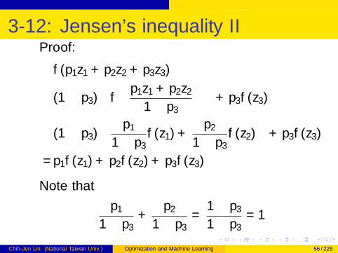
3-12: Jensen’s inequality IIProof:
f (p1z1 + p2z2 + p3z3)
≤(1− p3)
(f
(p1z1 + p2z2
1− p3
))+ p3f (z3)
≤(1− p3)
(p1
1− p3f (z1) +
p2
1− p3f (z2)
)+ p3f (z3)
=p1f (z1) + p2f (z2) + p3f (z3)
Note that
p1
1− p3+
p2
1− p3=
1− p3
1− p3= 1
Chih-Jen Lin (National Taiwan Univ.) Optimization and Machine Learning 56 / 228
3-14: Positive weighted sum &composition with affine function I
Composition with affine function:
We knowf (x) is convex
Isg(x) = f (Ax + b)
Chih-Jen Lin (National Taiwan Univ.) Optimization and Machine Learning 57 / 228
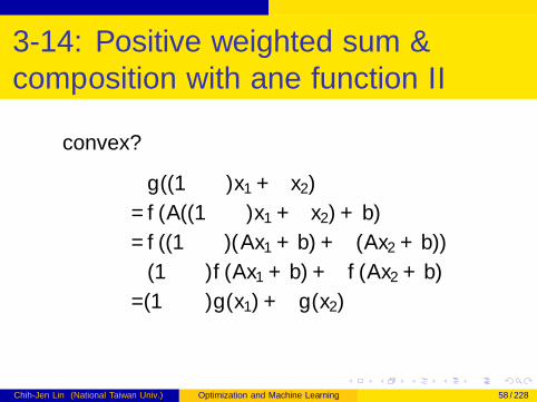
3-14: Positive weighted sum &composition with affine function II
convex?
g((1− α)x1 + αx2)
=f (A((1− α)x1 + αx2) + b)
=f ((1− α)(Ax1 + b) + α(Ax2 + b))
≤(1− α)f (Ax1 + b) + αf (Ax2 + b)
=(1− α)g(x1) + αg(x2)
Chih-Jen Lin (National Taiwan Univ.) Optimization and Machine Learning 58 / 228
3-15: Pointwise maximum I
Proof of the convexity
f ((1− α)x1 + αx2)
= max(f1((1− α)x1 + αx2), . . . , fm((1− α)x1 + αx2))
≤max((1− α)f1(x1) + αf1(x2), . . . ,
(1− α)fm(x1) + αfm(x2))
≤(1− α) max(f1(x1), . . . , fm(x1))+
αmax(f1(x2), . . . , fm(x2))
≤(1− α)f (x1) + αf (x2)
Chih-Jen Lin (National Taiwan Univ.) Optimization and Machine Learning 59 / 228
3-15: Pointwise maximum II
For
f (x) = x[1] + · · ·+ x[r ]
consider all (n
r
)combinations
Chih-Jen Lin (National Taiwan Univ.) Optimization and Machine Learning 60 / 228
3-16: Pointwise supremum I
The proof is similar to pointwise maximum
Support function of a set C :
When y is fixed,
f (x , y) = yTx
is linear (convex) in x
Maximum eigenvales of symmetric matrix
f (X , y) = yTXy
is a linear function of X when y is fixed
Chih-Jen Lin (National Taiwan Univ.) Optimization and Machine Learning 61 / 228
3-19: Minimization I
Proof:
Let ε > 0. ∃y1, y2 ∈ C such that
f (x1, y1) ≤ g(x1) + ε
f (x2, y2) ≤ g(x2) + ε
g(θx1 + (1− θ)x2) = infy∈C
f (θx1 + (1− θ)x2, y)
≤f (θx1 + (1− θ)x2, θy1 + (1− θ)y2)
≤θf (x1, y1) + (1− θ)f (x2, y2)
≤θg(x1) + (1− θ)g(x2) + εChih-Jen Lin (National Taiwan Univ.) Optimization and Machine Learning 62 / 228
3-19: Minimization II
Note that the first inequality use the peroperty thatC is convex to have
θy1 + (1− θ)y2 ∈ C
Because the above inequality holds for all ε > 0,
g(θx1 + (1− θ)x2) ≤ θg(x1) + (1− θ)g(x2)
First example:
Chih-Jen Lin (National Taiwan Univ.) Optimization and Machine Learning 63 / 228
3-19: Minimization III
The goal is to prove
A− BC−1BT � 0
Instead of a direct proof, here we use the propertyin this slide. First we have that f (x , y) is convex in(x , y) because [
A BBT C
]� 0
Considerminy
f (x , y)
Chih-Jen Lin (National Taiwan Univ.) Optimization and Machine Learning 64 / 228
3-19: Minimization IV
BecauseC � 0,
the minimum occurs at
2Cy + 2BTx = 0
y = −C−1BTx
Then
g(x) = xTAx − 2xTBC−1Bx + xTBC−1CC−1BTx
= xT (A− BC−1BT )x
Chih-Jen Lin (National Taiwan Univ.) Optimization and Machine Learning 65 / 228
3-19: Minimization V
is convex. The second-order condition implies that
A− BC−1BT � 0
Chih-Jen Lin (National Taiwan Univ.) Optimization and Machine Learning 66 / 228
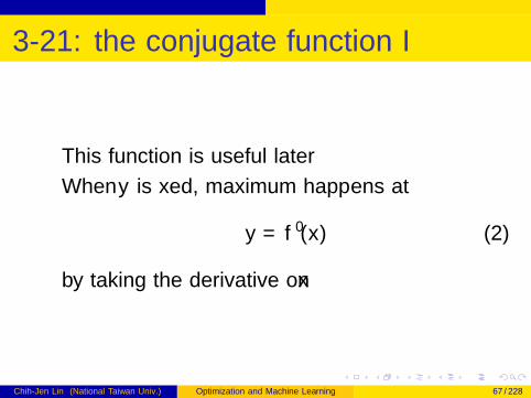
3-21: the conjugate function I
This function is useful later
When y is fixed, maximum happens at
y = f ′(x) (2)
by taking the derivative on x
Chih-Jen Lin (National Taiwan Univ.) Optimization and Machine Learning 67 / 228
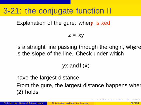
3-21: the conjugate function II
Explanation of the figure: when y is fixed
z = xy
is a straight line passing through the origin, where yis the slope of the line. Check under which x ,
yx and f (x)
have the largest distance
From the figure, the largest distance happens when(2) holds
Chih-Jen Lin (National Taiwan Univ.) Optimization and Machine Learning 68 / 228
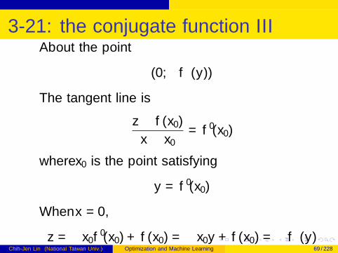
3-21: the conjugate function IIIAbout the point
(0,−f ∗(y))
The tangent line is
z − f (x0)
x − x0= f ′(x0)
where x0 is the point satisfying
y = f ′(x0)
When x = 0,
z = −x0f′(x0) + f (x0) = −x0y + f (x0) = −f ∗(y)
Chih-Jen Lin (National Taiwan Univ.) Optimization and Machine Learning 69 / 228
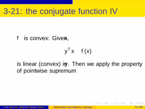
3-21: the conjugate function IV
f ∗ is convex: Given x ,
yTx − f (x)
is linear (convex) in y . Then we apply the propertyof pointwise supremum
Chih-Jen Lin (National Taiwan Univ.) Optimization and Machine Learning 70 / 228
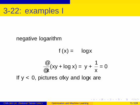
3-22: examples I
negative logarithm
f (x) = − log x
∂
∂x(xy + log x) = y +
1
x= 0
If y < 0, pictures of xy and log x are
Chih-Jen Lin (National Taiwan Univ.) Optimization and Machine Learning 71 / 228
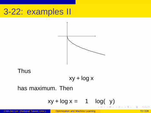
3-22: examples II
Thusxy + log x
has maximum. Then
xy + log x = −1− log(−y)
Chih-Jen Lin (National Taiwan Univ.) Optimization and Machine Learning 72 / 228
3-22: examples III
strictly convex quadratic
Qx = y , x = Q−1y
yTx − 1
2xTQx
=yTQ−1y − 1
2yTQ−1QQ−1y
=1
2yTQ−1y
Chih-Jen Lin (National Taiwan Univ.) Optimization and Machine Learning 73 / 228
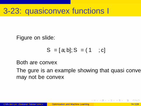
3-23: quasiconvex functions I
Figure on slide:
Sα = [a, b], Sβ = (−∞, c]
Both are convex
The figure is an example showing that quasi convexmay not be convex
Chih-Jen Lin (National Taiwan Univ.) Optimization and Machine Learning 74 / 228
3-26: properties of quasiconvex functions I
Modified Jensen inequality:f quasiconvex if and only if
f (θx+(1−θ)y) ≤ max{f (x), f (y)},∀x , y , θ ∈ [0, 1].
⇒ Let∆ = max{f (x), f (y)}
S∆ is convexx ∈ S∆, y ∈ S∆
θx + (1− θ)y ∈ S∆
Chih-Jen Lin (National Taiwan Univ.) Optimization and Machine Learning 75 / 228
3-26: properties of quasiconvex functionsII
f (θx + (1− θ)y) ≤ ∆
and the result is obtained
⇐ If results are wrong, there exists α such that Sαis not convex.
∃x , y , θ with x , y ∈ Sα, θ ∈ [0, 1] such that
θx + (1− θ)y /∈ Sα
Chih-Jen Lin (National Taiwan Univ.) Optimization and Machine Learning 76 / 228
3-26: properties of quasiconvex functionsIII
Then
f (θx + (1− θ)y) > α ≥ max{f (x), f (y)}
This violates the assumption
First-order condition (this is exercise 3.43):
Chih-Jen Lin (National Taiwan Univ.) Optimization and Machine Learning 77 / 228
3-26: properties of quasiconvex functionsIV
“⇒”
f ((1− t)x + ty) ≤ max(f (x), f (y)) = f (x)
f (x + t(y − x))− f (x)
t≤ 0
limt→0
f (x + t(y − x))− f (x)
t= ∇f (x)T (y − x) ≤ 0
Chih-Jen Lin (National Taiwan Univ.) Optimization and Machine Learning 78 / 228
3-26: properties of quasiconvex functionsV
⇐: If results are wrong, there exists α such that Sαis not convex.
∃x , y , θ with x , y ∈ Sα, θ ∈ [0, 1] such that
θx + (1− θ)y /∈ Sα
Then
f (θx + (1− θ)y) > α ≥ max{f (x), f (y)} (3)
Chih-Jen Lin (National Taiwan Univ.) Optimization and Machine Learning 79 / 228
3-26: properties of quasiconvex functionsVI
Because f is differentiable, it is continuous.Without loss of generality, we have
f (z) ≥ f (x), f (y),∀z between x and y (4)
Let’s give a 1-D interpretation. From (3), we canfind a ball surrounding
θx + (1− θ)y
Chih-Jen Lin (National Taiwan Univ.) Optimization and Machine Learning 80 / 228
3-26: properties of quasiconvex functionsVII
and two points x ′, y ′ such that
f (z) ≥ f (x ′) = f (y ′),∀z between x ′ and y ′
With (4),
z = x + θ(y − x), θ ∈ (0, 1)
∇f (z)T (−θ(y − x)) ≤ 0
∇f (z)T (y − x − θ(y − x)) ≤ 0
Chih-Jen Lin (National Taiwan Univ.) Optimization and Machine Learning 81 / 228
3-26: properties of quasiconvex functionsVIII
Then∇f (z)T (y − x) = 0,∀θ ∈ (0, 1)
f (x + θ(y − x))
=f (x) +∇f (t)Tθ(y − x)
=f (x),∀θ ∈ [0, 1)
This contradicts (3).
Chih-Jen Lin (National Taiwan Univ.) Optimization and Machine Learning 82 / 228
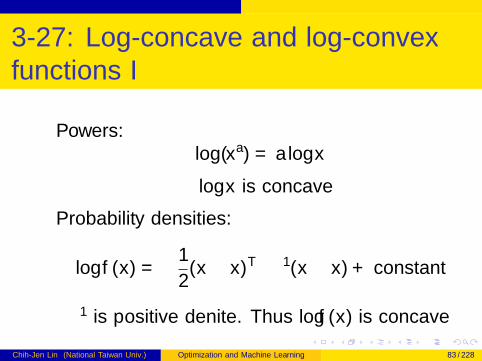
3-27: Log-concave and log-convexfunctions I
Powers:log(xa) = a log x
log x is concave
Probability densities:
log f (x) = −1
2(x − x)TΣ−1(x − x) + constant
Σ−1 is positive definite. Thus log f (x) is concave
Chih-Jen Lin (National Taiwan Univ.) Optimization and Machine Learning 83 / 228
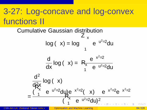
3-27: Log-concave and log-convexfunctions II
Cumulative Gaussian distribution
log Φ(x) = log
∫ x
−∞e−u
2/2du
d
dxlog Φ(x) =
e−x2/2∫ x
−∞ e−u2/2du
d2
d2xlog Φ(x)
=(∫ x
−∞ e−u2/2du)e−x
2/2(−x)− e−x2/2e−x
2/2
(∫ x
−∞ e−u2/2du)2
Chih-Jen Lin (National Taiwan Univ.) Optimization and Machine Learning 84 / 228
3-27: Log-concave and log-convexfunctions III
Need to prove that(∫ x
−∞e−u
2/2du
)x + e−x
2/2 > 0
Because
x ≥ u for all u ∈ (−∞, x ],
Chih-Jen Lin (National Taiwan Univ.) Optimization and Machine Learning 85 / 228
3-27: Log-concave and log-convexfunctions IV
we have (∫ x
−∞e−u
2/2du
)x + e−x
2/2
=
∫ x
−∞xe−u
2/2du + e−x2/2
≥∫ x
−∞ue−u
2/2du + e−x2/2
=− e−u2/2|x−∞ + e−x
2/2
=− e−x2/2 + e−x
2/2 = 0
Chih-Jen Lin (National Taiwan Univ.) Optimization and Machine Learning 86 / 228
3-27: Log-concave and log-convexfunctions V
This proof was given by a student (and polished byanother student) of this course before
Chih-Jen Lin (National Taiwan Univ.) Optimization and Machine Learning 87 / 228
4-3: Optimal and locally optimal points I
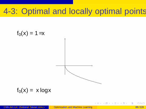
f0(x) = 1/x
f0(x) = x log x
Chih-Jen Lin (National Taiwan Univ.) Optimization and Machine Learning 88 / 228
4-3: Optimal and locally optimal points II
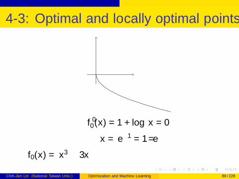
f ′0(x) = 1 + log x = 0
x = e−1 = 1/e
f0(x) = x3 − 3x
Chih-Jen Lin (National Taiwan Univ.) Optimization and Machine Learning 89 / 228
4-3: Optimal and locally optimal points III
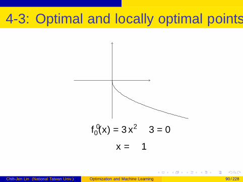
f ′0(x) = 3x2 − 3 = 0
x = ±1
Chih-Jen Lin (National Taiwan Univ.) Optimization and Machine Learning 90 / 228
4-7: example I
x1/(1 + x22 ) ≤ 0
⇔ x1 ≤ 0
(x1 + x2)2 = 0
⇔ x1 + x2 = 0
Chih-Jen Lin (National Taiwan Univ.) Optimization and Machine Learning 91 / 228
4-9: Optimality criterion for differentiablef0 I
⇐: easyFrom first-order condition
f0(y) ≥ f0(x) +∇f0(x)T (y − x)
Together with
∇f0(x)T (y − x) ≥ 0
we have
f0(y) ≥ f0(x), for all feasible yChih-Jen Lin (National Taiwan Univ.) Optimization and Machine Learning 92 / 228
4-9: Optimality criterion for differentiablef0 II
⇒ Assume the result is wrong. Then
∇f0(x)T (y − x) < 0
Letz(t) = ty + (1− t)x
d
dtf0(z(t)) = ∇f0(z(t))T (y − x)
d
dtf0(z(t))
∣∣∣∣t=0
= ∇f0(x)T (y − x) < 0
Chih-Jen Lin (National Taiwan Univ.) Optimization and Machine Learning 93 / 228
4-9: Optimality criterion for differentiablef0 III
There exists t such that
f0(z(t)) < f0(x)
Note thatz(t)
is feasible because
fi(z(t)) ≤ tfi(x) + (1− t)fi(y) ≤ 0
and
A(tx+(1−t)y) = tAx+(1−t)Ay = tb+(1−b)b = bChih-Jen Lin (National Taiwan Univ.) Optimization and Machine Learning 94 / 228
4-9: Optimality criterion for differentiablef0 IV
Chih-Jen Lin (National Taiwan Univ.) Optimization and Machine Learning 95 / 228
4-10 I
Unconstrained problem:
Lety = x − t∇f0(x)
It is feasible (unconstrained problem). Optimalitycondition implies
∇f0(x)T (y − x) = −t‖∇f0(x)‖2 ≥ 0
Thus∇f0(x) = 0
Equality constrained problemChih-Jen Lin (National Taiwan Univ.) Optimization and Machine Learning 96 / 228
4-10 II
⇐ Easy. For any feasible y ,
Ay = b
∇f0(x)T (y−x) = −νTA(y−x) = −νT (b−b) = 0 ≥ 0
So x is optimal
⇒: more complicated. We only do a roughexplanation
Chih-Jen Lin (National Taiwan Univ.) Optimization and Machine Learning 97 / 228
4-10 III
From optimality condition
∇f0(x)Tν = ∇f0(x)T ((x + ν)− x) ≥ 0,∀ν ∈ N(A)
N(A) is a subspace in 2-D. Thus
ν ∈ N(A)⇒ −ν ∈ N(A)
Chih-Jen Lin (National Taiwan Univ.) Optimization and Machine Learning 98 / 228
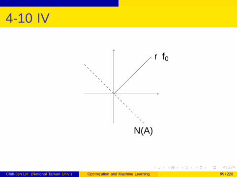
4-10 IV
N(A)
∇f0
Chih-Jen Lin (National Taiwan Univ.) Optimization and Machine Learning 99 / 228
4-10 V
We have
∇f0(x)Tν = 0,∀ν ∈ N(A)
∇f0(x) ⊥ N(A),∇f0(x) ∈ R(AT )
⇒ ∃ν such that ∇f0(x) + ATν = 0
Minimization over nonnegative orthant
⇐ Easy
Chih-Jen Lin (National Taiwan Univ.) Optimization and Machine Learning 100 / 228
4-10 VI
For any y � 0,
∇i f0(x)(yi − xi) =
{∇i f0(x)yi ≥ 0 if xi = 0
0 if xi > 0.
Therefore,∇f0(x)T (y − x) ≥ 0
andx is optimal
Chih-Jen Lin (National Taiwan Univ.) Optimization and Machine Learning 101 / 228
4-10 VII
⇒ If xi = 0, we claim
∇i f0(x) ≥ 0
Otherwise,∇i f0(x) < 0
Lety = x except yi →∞
∇f0(x)T (y − x) = ∇i f0(x)(yi − xi)→ −∞This violates the optimality condition
Chih-Jen Lin (National Taiwan Univ.) Optimization and Machine Learning 102 / 228
4-10 VIII
If xi > 0, we claim
∇i f0(x) = 0
Otherwise, assume
∇i f0(x) > 0
Consider
y = x except yi = xi/2 > 0
Chih-Jen Lin (National Taiwan Univ.) Optimization and Machine Learning 103 / 228
4-10 IX
It is feasible. Then
∇f0(x)T (y−x) = ∇i f0(x)(yi−xi) = −∇i f0(x)xi/2 < 0
violates the optimality condition. The situation for
∇i f0(x) < 0
is similar
Chih-Jen Lin (National Taiwan Univ.) Optimization and Machine Learning 104 / 228
4-23: examples I
least-squares
min xT (ATA)x − 2bTAx + bTb
ATA may not be invertibe ⇒ pseudo inverse
linear program with random cost
c ≡ E (C )
Σ ≡ EC ((C − c)(C − c)T )
Chih-Jen Lin (National Taiwan Univ.) Optimization and Machine Learning 105 / 228
4-23: examples II
Var(CTx) = EC ((CTx − cTx)(CTx − cTx))
= EC (xT (C − c)(C − c)Tx)
= xTΣx
Chih-Jen Lin (National Taiwan Univ.) Optimization and Machine Learning 106 / 228
4-25: second-order cone programming I
Cone was defined on slide 2-8
{(x , t) | ‖x‖ ≤ t}
Chih-Jen Lin (National Taiwan Univ.) Optimization and Machine Learning 107 / 228
4-35: generalized inequality constraint I
fi ∈ Rn → Rki Ki -convex:
fi(θx + (1− θ)y) �Kiθfi(x) + (1− θ)fi(y)
See page 3-31
Chih-Jen Lin (National Taiwan Univ.) Optimization and Machine Learning 108 / 228
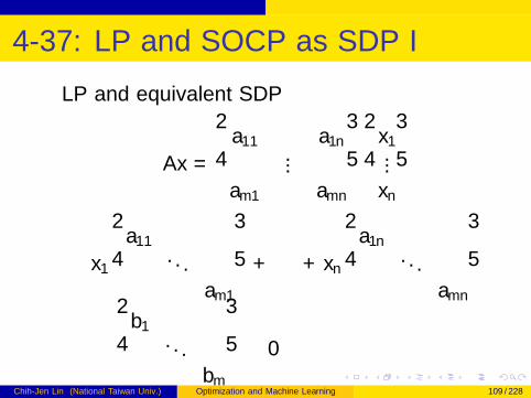
4-37: LP and SOCP as SDP I
LP and equivalent SDP
Ax =
a11 · · · a1n...
am1 · · · amn
x1...xn
x1
a11. . .
am1
+ · · ·+ xn
a1n. . .
amn
−
b1. . .
bm
� 0
Chih-Jen Lin (National Taiwan Univ.) Optimization and Machine Learning 109 / 228
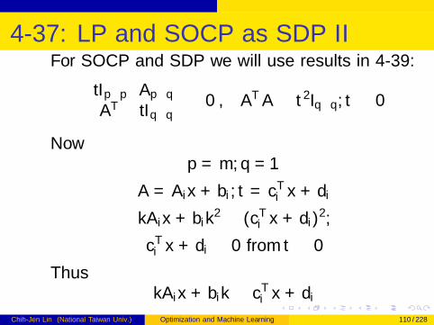
4-37: LP and SOCP as SDP IIFor SOCP and SDP we will use results in 4-39:[
tIp×p Ap×qAT tIq×q
]� 0⇔ ATA � t2Iq×q, t ≥ 0
Nowp = m, q = 1
A = Aix + bi , t = cTi x + di
‖Aix + bi‖2 ≤ (cTi x + di)2,
cTi x + di ≥ 0 from t ≥ 0
Thus‖Aix + bi‖ ≤ cTi x + di
Chih-Jen Lin (National Taiwan Univ.) Optimization and Machine Learning 110 / 228
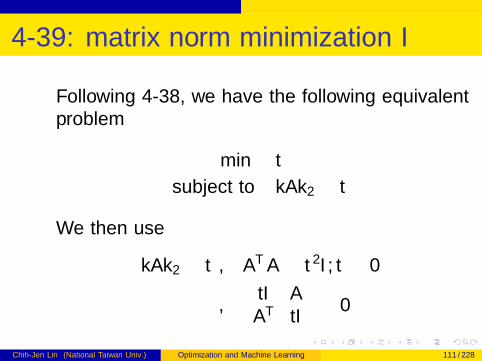
4-39: matrix norm minimization I
Following 4-38, we have the following equivalentproblem
min t
subject to ‖A‖2 ≤ t
We then use
‖A‖2 ≤ t ⇔ ATA � t2I , t ≥ 0
⇔[tI AAT tI
]� 0
Chih-Jen Lin (National Taiwan Univ.) Optimization and Machine Learning 111 / 228
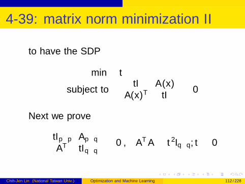
4-39: matrix norm minimization II
to have the SDP
min t
subject to
[tI A(x)
A(x)T tI
]� 0
Next we prove[tIp×p Ap×qAT tIq×q
]� 0⇔ ATA � t2Iq×q, t ≥ 0
Chih-Jen Lin (National Taiwan Univ.) Optimization and Machine Learning 112 / 228
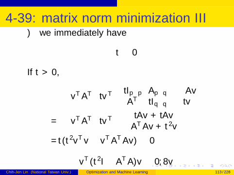
4-39: matrix norm minimization III⇒ we immediately have
t ≥ 0
If t > 0,[−vTAT tvT
] [tIp×p Ap×qAT tIq×q
] [−Avtv
]=[−vTAT tvT
] [ −tAv + tAv−ATAv + t2v
]=t(t2vTv − vTATAv) ≥ 0
vT (t2I − ATA)v ≥ 0,∀vChih-Jen Lin (National Taiwan Univ.) Optimization and Machine Learning 113 / 228
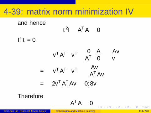
4-39: matrix norm minimization IVand hence
t2I − ATA � 0
If t = 0 [−vTAT vT
] [ 0 AAT 0
] [−Avv
]=[−vTAT vT
] [ Av−ATAv
]=− 2vTATAv ≥ 0,∀v
ThereforeATA � 0
Chih-Jen Lin (National Taiwan Univ.) Optimization and Machine Learning 114 / 228
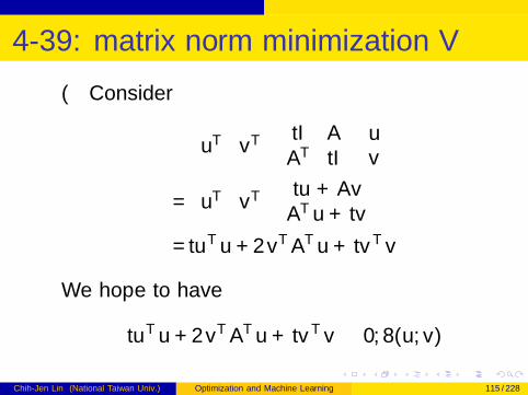
4-39: matrix norm minimization V
⇐ Consider [uT vT
] [ tI AAT tI
] [uv
]=[uT vT
] [ tu + AvATu + tv
]=tuTu + 2vTATu + tvTv
We hope to have
tuTu + 2vTATu + tvTv ≥ 0,∀(u, v)
Chih-Jen Lin (National Taiwan Univ.) Optimization and Machine Learning 115 / 228
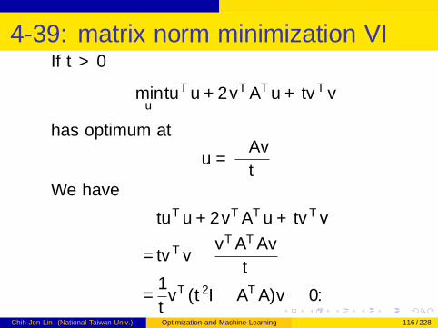
4-39: matrix norm minimization VIIf t > 0
minu
tuTu + 2vTATu + tvTv
has optimum at
u =−Avt
We have
tuTu + 2vTATu + tvTv
=tvTv − vTATAv
t
=1
tvT (t2I − ATA)v ≥ 0.
Chih-Jen Lin (National Taiwan Univ.) Optimization and Machine Learning 116 / 228
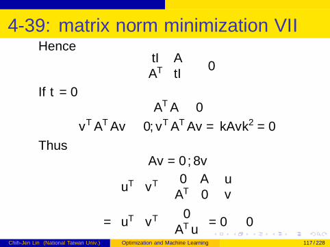
4-39: matrix norm minimization VIIHence [
tI AAT tI
]� 0
If t = 0ATA � 0
vTATAv ≤ 0, vTATAv = ‖Av‖2 = 0
ThusAv = 0,∀v[
uT vT] [ 0 A
AT 0
] [uv
]=[uT vT
] [ 0ATu
]= 0 ≥ 0
Chih-Jen Lin (National Taiwan Univ.) Optimization and Machine Learning 117 / 228
4-39: matrix norm minimization VIII
Thus [0 AAT 0
]� 0
Chih-Jen Lin (National Taiwan Univ.) Optimization and Machine Learning 118 / 228
4-40: Vector optimization I
Though
f0(x) is a vector
note that
fi(x) is still Rn → R1
K -convex
See 3-31 though we didn’t discuss it earlier
f0(θx + (1− θ)y) �K θf0(x) + (1− θ)f0(y)
Chih-Jen Lin (National Taiwan Univ.) Optimization and Machine Learning 119 / 228
4-41: optimal and pareto optimal points I
See definition in slide 2-38
OptimalO ⊆ {x}+ K
Pareto optimal
(x − K ) ∩ O = {x}
Chih-Jen Lin (National Taiwan Univ.) Optimization and Machine Learning 120 / 228
5-3: Lagrange dual function I
Note that g is concave no matter if the originalproblem is convex or not
f0(x) +∑
λi fi(x) +∑
νihi(x)
is convex (linear) in λ, ν for each x
Chih-Jen Lin (National Taiwan Univ.) Optimization and Machine Learning 121 / 228
5-3: Lagrange dual function IIUse pointwise supremum on 3-16
supx∈D
(−f0(x)−∑
λi fi(x)−∑
νihi(x))
is convex. Hence
inf(f0(x) +∑
λi fi(x) +∑
νihi(x))
is concave. Note that
− sup(− · · · ) = −convex
= inf(· · · ) = concave
Chih-Jen Lin (National Taiwan Univ.) Optimization and Machine Learning 122 / 228
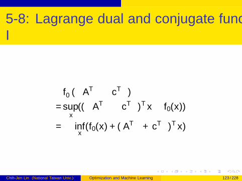
5-8: Lagrange dual and conjugate functionI
f ∗0 (−ATλ− cTν)
= supx
((−ATλ− cTν)Tx − f0(x))
=− infx
(f0(x) + (ATλ + cTν)Tx)
Chih-Jen Lin (National Taiwan Univ.) Optimization and Machine Learning 123 / 228
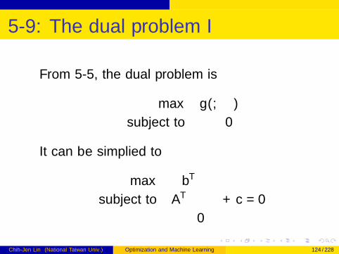
5-9: The dual problem I
From 5-5, the dual problem is
max g(λ, ν)
subject to λ � 0
It can be simplified to
max −bTνsubject to ATν − λ + c = 0
λ � 0
Chih-Jen Lin (National Taiwan Univ.) Optimization and Machine Learning 124 / 228
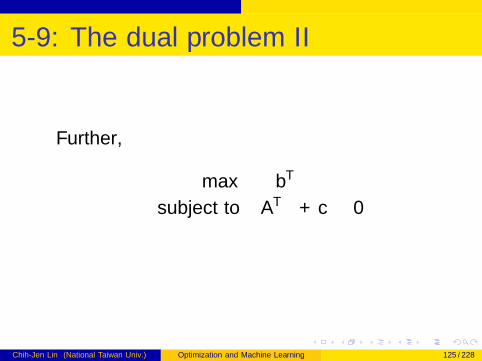
5-9: The dual problem II
Further,
max −bTνsubject to ATν + c � 0
Chih-Jen Lin (National Taiwan Univ.) Optimization and Machine Learning 125 / 228

5-10: weak and strong duality I
We don’t discuss the SDP problem on this slidebecause we omitted 5-7 on the two-way partitioningproblem
Chih-Jen Lin (National Taiwan Univ.) Optimization and Machine Learning 126 / 228
5-11: Slater’s constraint qualification I
We omit the proof because of no time
“linear inequality do not need to hold with strictinequality”: for linear inequalities we DO NOT needconstraint qualification
We will see some explanation later
Chih-Jen Lin (National Taiwan Univ.) Optimization and Machine Learning 127 / 228
5-12: inequality from LP I
If we have only linear constraints, then constraintqualification holds
Chih-Jen Lin (National Taiwan Univ.) Optimization and Machine Learning 128 / 228
5-15: geometric interpretation I
Explanation of g(λ): when λ is fixed
λu + t = ∆
is a line. We lower ∆ until it touches the boundaryof G
The ∆ value then becomes g(λ)
Whenu = 0⇒ t = ∆
so we see the point marked as g(λ) on t-axis
Chih-Jen Lin (National Taiwan Univ.) Optimization and Machine Learning 129 / 228
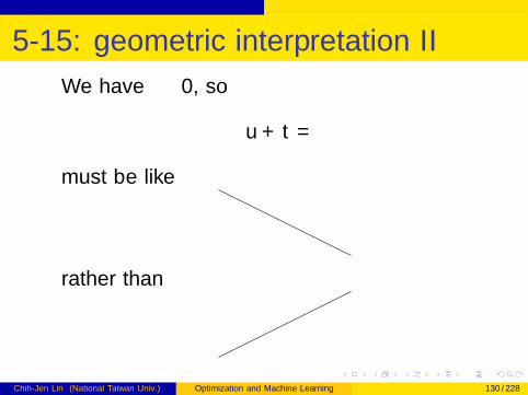
5-15: geometric interpretation II
We have λ ≥ 0, so
λu + t = ∆
must be like
rather than
Chih-Jen Lin (National Taiwan Univ.) Optimization and Machine Learning 130 / 228
5-15: geometric interpretation III
Explanation of p∗:
In G , only points satisfying
u ≤ 0
are feasible
Chih-Jen Lin (National Taiwan Univ.) Optimization and Machine Learning 131 / 228
5-16 I
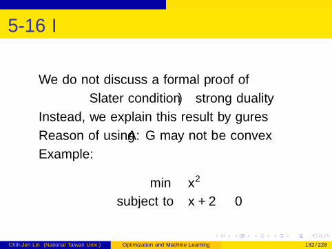
We do not discuss a formal proof of
Slater condition ⇒ strong duality
Instead, we explain this result by figures
Reason of using A: G may not be convex
Example:
min x2
subject to x + 2 ≤ 0
Chih-Jen Lin (National Taiwan Univ.) Optimization and Machine Learning 132 / 228
5-16 II
This is a convex optimization problem
G = {(x + 2, x2) | x ∈ R}
is only a quadratic curve
Chih-Jen Lin (National Taiwan Univ.) Optimization and Machine Learning 133 / 228
5-16 III
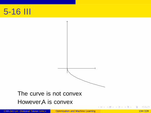
The curve is not convex
However, A is convex
Chih-Jen Lin (National Taiwan Univ.) Optimization and Machine Learning 134 / 228
5-16 IV
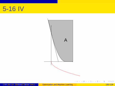
A
Chih-Jen Lin (National Taiwan Univ.) Optimization and Machine Learning 135 / 228
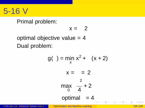
5-16 VPrimal problem:
x = −2
optimal objective value = 4
Dual problem:
g(λ) = minx
x2 + λ(x + 2)
x = −λ/2
maxλ≥0−λ
2
4+ 2λ
optimal λ = 4
Chih-Jen Lin (National Taiwan Univ.) Optimization and Machine Learning 136 / 228
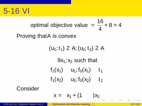
5-16 VI
optimal objective value = −16
4+ 8 = 4
Proving that A is convex
(u1, t1) ∈ A, (u2, t2) ∈ A
∃x1, x2 such that
f1(x1) ≤ u1, f0(x1) ≤ t1
f1(x2) ≤ u2, f0(x2) ≤ t2
Considerx = θx1 + (1− θ)x2
Chih-Jen Lin (National Taiwan Univ.) Optimization and Machine Learning 137 / 228
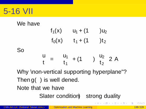
5-16 VII
We havef1(x) ≤ θu1 + (1− θ)u2
f0(x) ≤ θt1 + (1− θ)t2
So [ut
]= θ
[u1
t1
]+ (1− θ)
[u2
t2
]∈ A
Why “non-vertical supporting hyperplane”?
Then g(λ) is well defined.
Note that we have
Slater condition ⇒ strong duality
Chih-Jen Lin (National Taiwan Univ.) Optimization and Machine Learning 138 / 228
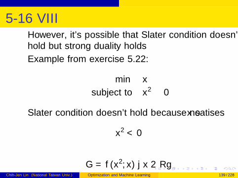
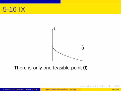
5-16 VIIIHowever, it’s possible that Slater condition doesn’thold but strong duality holds
Example from exercise 5.22:
min x
subject to x2 ≤ 0
Slater condition doesn’t hold because no x satisfies
x2 < 0
G = {(x2, x) | x ∈ R}Chih-Jen Lin (National Taiwan Univ.) Optimization and Machine Learning 139 / 228
5-16 IX
u
t
There is only one feasible point (0, 0)
Chih-Jen Lin (National Taiwan Univ.) Optimization and Machine Learning 140 / 228
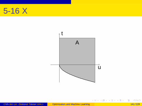
5-16 X
u
t
A
Chih-Jen Lin (National Taiwan Univ.) Optimization and Machine Learning 141 / 228
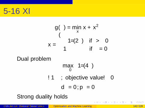
5-16 XI
g(λ) = minx
x + x2λ
x =
{−1/(2λ) if λ > 0
−∞ if λ = 0
Dual problemmaxλ≥0−1/(4λ)
λ→∞, objective value → 0
d∗ = 0, p∗ = 0
Strong duality holds
Chih-Jen Lin (National Taiwan Univ.) Optimization and Machine Learning 142 / 228
5-17: complementary slackness I
In deriving the inequality we use
hi(x∗) = 0 and fi(x
∗) ≤ 0
Complementary slackness
compare the earlier results in 4-10
Chih-Jen Lin (National Taiwan Univ.) Optimization and Machine Learning 143 / 228
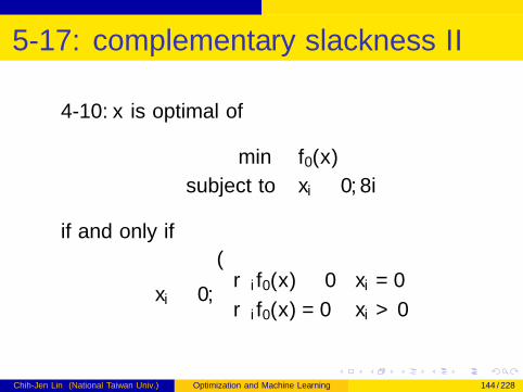
5-17: complementary slackness II
4-10: x is optimal of
min f0(x)
subject to xi ≥ 0,∀i
if and only if
xi ≥ 0,
{∇i f0(x) ≥ 0 xi = 0
∇i f0(x) = 0 xi > 0
Chih-Jen Lin (National Taiwan Univ.) Optimization and Machine Learning 144 / 228
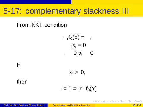
5-17: complementary slackness III
From KKT condition
∇i f0(x) = λiλixi = 0
λi ≥ 0, xi ≥ 0
Ifxi > 0,
thenλi = 0 = ∇i f0(x)
Chih-Jen Lin (National Taiwan Univ.) Optimization and Machine Learning 145 / 228
5-19: KKT conditions for convex problemI
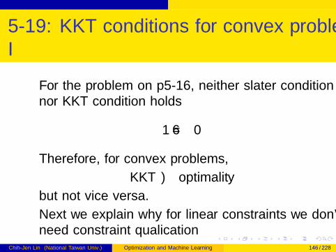
For the problem on p5-16, neither slater conditionnor KKT condition holds
1 6= λ0
Therefore, for convex problems,
KKT ⇒ optimality
but not vice versa.
Next we explain why for linear constraints we don’tneed constraint qualification
Chih-Jen Lin (National Taiwan Univ.) Optimization and Machine Learning 146 / 228
5-19: KKT conditions for convex problemII
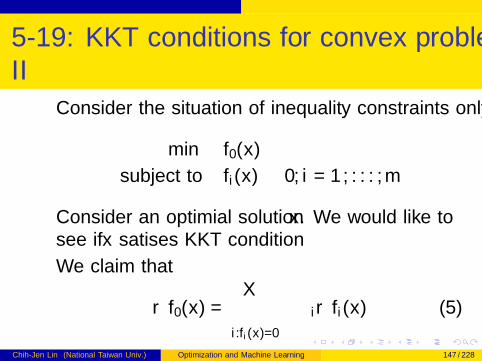
Consider the situation of inequality constraints only:
min f0(x)
subject to fi(x) ≤ 0, i = 1, . . . ,m
Consider an optimial solution x . We would like tosee if x satisfies KKT condition
We claim that
∇f0(x) =∑
i :fi (x)=0
−λi∇fi(x) (5)
Chih-Jen Lin (National Taiwan Univ.) Optimization and Machine Learning 147 / 228
5-19: KKT conditions for convex problemIII
Assume the result is wrong. Then,
∇f0(x) =linear combination of {∇fi(x) | fi(x) = 0}+ ∆,
where
∆ 6= 0 and ∆T∇fi(x) = 0,∀i : fi(x) = 0
Chih-Jen Lin (National Taiwan Univ.) Optimization and Machine Learning 148 / 228
5-19: KKT conditions for convex problemIV
Then there exists α < 0 such that
δx ≡ α∆
satisfies∇fi(x)Tδx = 0 if fi(x) = 0
andfi(x + δx) ≤ 0 if fi(x) < 0
We claim that δx is feasible. That is,
fi(x + δx) ≤ 0,∀iChih-Jen Lin (National Taiwan Univ.) Optimization and Machine Learning 149 / 228
5-19: KKT conditions for convex problemV
We have
fi(x + δx) ≈ fi(x) +∇fi(x)Tδx = 0 if fi(x) = 0
However,
∇f0(x)Tδx = α∆T∆ < 0
This contradicts the optimality condition that fromslide 4-9, for any feasible direction δx ,
∇f0(x)Tδx ≥ 0.Chih-Jen Lin (National Taiwan Univ.) Optimization and Machine Learning 150 / 228
5-19: KKT conditions for convex problemVI
We do not continue to prove
∇f0(x) =∑
λi≥0,fi (x)=0
−λi∇fi(x) (6)
because the proof is not trivial
However, what we want to say is that in proving(5), the proof is not rigourous because of ≈For linear the proof becomes rigourous
This roughly give you a feeling that linear isdifferent from non-linear
Chih-Jen Lin (National Taiwan Univ.) Optimization and Machine Learning 151 / 228
5-25 I
Explanation of f ∗0 (ν)
infy
(f0(y)− νTy)
=− supy
(νTy − f0(y)) = −f ∗0 (ν)
where f ∗0 (ν) is the conjugate function
Chih-Jen Lin (National Taiwan Univ.) Optimization and Machine Learning 152 / 228
5-26 I
The original problem
g(λ, ν) = infx‖Ax − b‖ = constant
Dual norm:
‖ν‖∗ ≡ sup{νTy | ‖y‖ ≤ 1}
If ‖ν‖∗ > 1,
νTy ∗ > 1, ‖y ∗‖ ≤ 1
Chih-Jen Lin (National Taiwan Univ.) Optimization and Machine Learning 153 / 228
5-26 IIinf ‖y‖+ νTy
≤‖ − y ∗‖ − νTy ∗ < 0
‖ − ty ∗‖ − νT (ty ∗)→ −∞ as t →∞Hence
infy‖y‖+ νTy = −∞
If ‖ν‖∗ ≤ 1, we claim that
infy‖y‖+ νTy = 0
y = 0⇒ ‖y‖+ νTy = 0
Chih-Jen Lin (National Taiwan Univ.) Optimization and Machine Learning 154 / 228
5-26 III
If ∃y such that
‖y‖+ νTy < 0
then‖ − y‖ < −νTy
We can scale y so that
sup{νTy | ‖y‖ ≤ 1} > 1
but this causes a contradiction
Chih-Jen Lin (National Taiwan Univ.) Optimization and Machine Learning 155 / 228
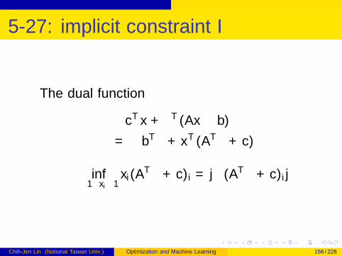
5-27: implicit constraint I
The dual function
cTx + νT (Ax − b)
=− bTν + xT (ATν + c)
inf−1≤xi≤1
xi(ATν + c)i = −|(ATν + c)i |
Chih-Jen Lin (National Taiwan Univ.) Optimization and Machine Learning 156 / 228
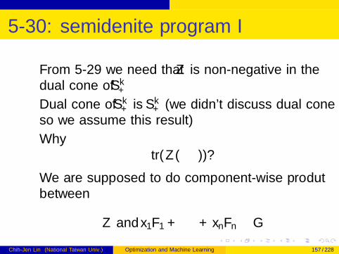
5-30: semidefinite program I
From 5-29 we need that Z is non-negative in thedual cone of Sk
+
Dual cone of Sk+ is Sk
+ (we didn’t discuss dual coneso we assume this result)
Whytr(Z (· · · ))?
We are supposed to do component-wise produtbetween
Z and x1F1 + · · ·+ xnFn − G
Chih-Jen Lin (National Taiwan Univ.) Optimization and Machine Learning 157 / 228
5-30: semidefinite program II
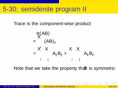
Trace is the component-wise product
tr(AB)
=∑i
(AB)ii
=∑i
∑j
AijBji =∑i
∑j
AijBij
Note that we take the property that B is symmetric
Chih-Jen Lin (National Taiwan Univ.) Optimization and Machine Learning 158 / 228
7-4 I
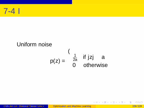
Uniform noise
p(z) =
{1
2a if |z | ≤ a
0 otherwise
Chih-Jen Lin (National Taiwan Univ.) Optimization and Machine Learning 159 / 228
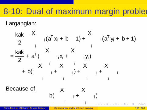
8-10: Dual of maximum margin problem I
Largangian:
‖a‖2−∑i
λi(aTxi + b − 1) +
∑i
µi(aTyi + b + 1)
=‖a‖
2+ aT (−
∑i
λixi +∑i
µiyi)
+ b(−∑i
λi +∑i
µi) +∑i
λi +∑i
µi
Because ofb(−
∑i
λi +∑i
µi)
Chih-Jen Lin (National Taiwan Univ.) Optimization and Machine Learning 160 / 228
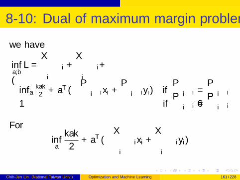
8-10: Dual of maximum margin problem II
we have
infa,b
L =∑i
λi +∑i
µi+{infa
‖a‖2 + aT (−
∑i λixi +
∑i µiyi) if
∑i λi =
∑i µi
−∞ if∑
i λi 6=∑
i µi
For
infa
‖a‖2
+ aT (−∑i
λixi +∑i
µiyi)
Chih-Jen Lin (National Taiwan Univ.) Optimization and Machine Learning 161 / 228
8-10: Dual of maximum margin problemIII
we can denote it as
infa
‖a‖2
+ vTa
where v is a vector. We cannot do derivative because‖a‖ is not differentiable. Formal solution:
Chih-Jen Lin (National Taiwan Univ.) Optimization and Machine Learning 162 / 228
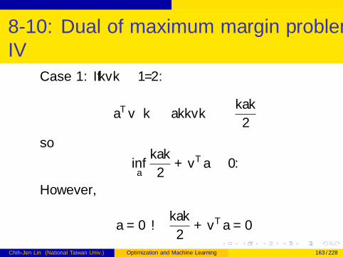
8-10: Dual of maximum margin problemIV
Case 1: If ‖v‖ ≤ 1/2:
aTv ≥ −‖a‖‖v‖ ≥ −‖a‖2
so
infa
‖a‖2
+ vTa ≥ 0.
However,
a = 0→ ‖a‖2
+ vTa = 0
Chih-Jen Lin (National Taiwan Univ.) Optimization and Machine Learning 163 / 228
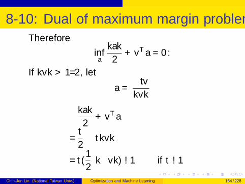
8-10: Dual of maximum margin problem VTherefore
infa
‖a‖2
+ vTa = 0.
If ‖v‖ > 1/2, let
a =−tv‖v‖
‖a‖2
+ vTa
=t
2− t‖v‖
=t(1
2− ‖v‖)→ −∞ if t →∞
Chih-Jen Lin (National Taiwan Univ.) Optimization and Machine Learning 164 / 228
8-10: Dual of maximum margin problemVI
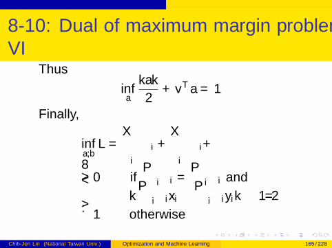
Thus
infa
‖a‖2
+ vTa = −∞
Finally,
infa,b
L =∑i
λi +∑i
µi+0 if
∑i λi =
∑i µi and
‖∑
i λixi −∑
i µiyi‖ ≤ 1/2
−∞ otherwise
Chih-Jen Lin (National Taiwan Univ.) Optimization and Machine Learning 165 / 228
8-14
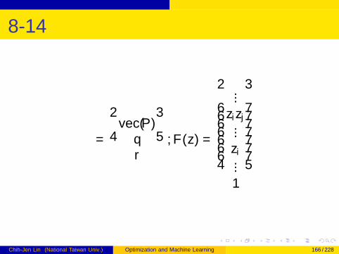
θ =
vec(P)qr
,F (z) =
...zizj
...zi...1
Chih-Jen Lin (National Taiwan Univ.) Optimization and Machine Learning 166 / 228
10-3: initial point and sublevel set I
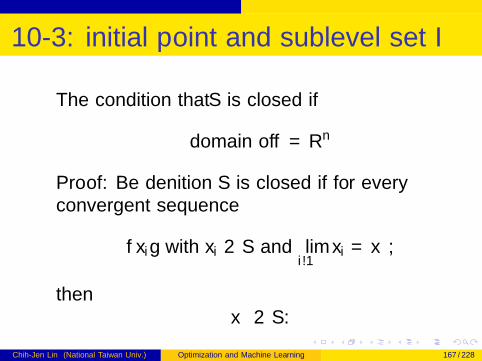
The condition that S is closed if
domain of f = Rn
Proof: Be definition S is closed if for everyconvergent sequence
{xi} with xi ∈ S and limi→∞
xi = x∗,
thenx∗ ∈ S .
Chih-Jen Lin (National Taiwan Univ.) Optimization and Machine Learning 167 / 228
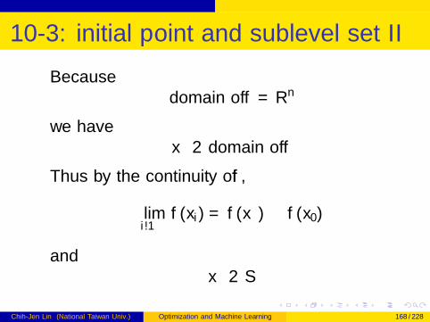
10-3: initial point and sublevel set II
Becausedomain of f = Rn
we havex∗ ∈ domain of f
Thus by the continuity of f ,
limi→∞
f (xi) = f (x∗) ≤ f (x0)
andx∗ ∈ S
Chih-Jen Lin (National Taiwan Univ.) Optimization and Machine Learning 168 / 228
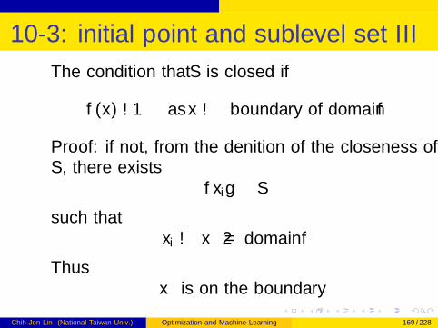
10-3: initial point and sublevel set III
The condition that S is closed if
f (x)→∞ as x → boundary of domain f
Proof: if not, from the definition of the closeness ofS , there exists
{xi} ⊂ S
such thatxi → x∗ /∈ domain f
Thusx∗ is on the boundary
Chih-Jen Lin (National Taiwan Univ.) Optimization and Machine Learning 169 / 228
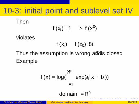
10-3: initial point and sublevel set IV
Thenf (xi)→∞ > f (x0)
violatesf (xi) ≤ f (x0),∀i
Thus the assumption is wrong and S is closed
Example
f (x) = log(m∑i=1
exp(aTi x + bi))
domain = Rn
Chih-Jen Lin (National Taiwan Univ.) Optimization and Machine Learning 170 / 228
10-3: initial point and sublevel set V
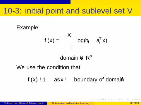
Example
f (x) = −∑i
log(bi − aTi x)
domain 6= Rn
We use the condition that
f (x)→∞ as x → boundary of domain f
Chih-Jen Lin (National Taiwan Univ.) Optimization and Machine Learning 171 / 228
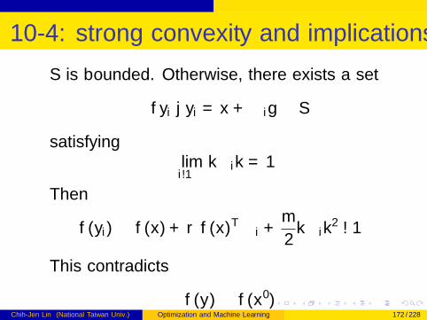
10-4: strong convexity and implications I
S is bounded. Otherwise, there exists a set
{yi | yi = x + ∆i} ⊂ S
satisfyinglimi→∞‖∆i‖ =∞
Then
f (yi) ≥ f (x) +∇f (x)T∆i +m
2‖∆i‖2 →∞
This contradicts
f (y) ≤ f (x0)Chih-Jen Lin (National Taiwan Univ.) Optimization and Machine Learning 172 / 228
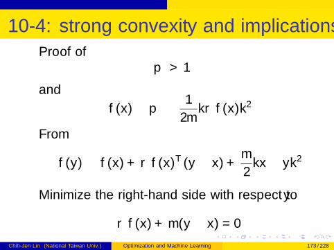
10-4: strong convexity and implications IIProof of
p∗ > −∞and
f (x)− p∗ ≤ 1
2m‖∇f (x)‖2
From
f (y) ≥ f (x) +∇f (x)T (y − x) +m
2‖x − y‖2
Minimize the right-hand side with respect to y
∇f (x) + m(y − x) = 0
Chih-Jen Lin (National Taiwan Univ.) Optimization and Machine Learning 173 / 228
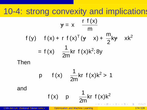
10-4: strong convexity and implications III
y = x − ∇f (x)
m
f (y) ≥ f (x) +∇f (x)T (y − x) +m
2‖y − x‖2
= f (x)− 1
2m‖∇f (x)‖2,∀y
Then
p∗ ≥ f (x)− 1
2m‖∇f (x)‖2 > −∞
and
f (x)− p∗ ≤ 1
2m‖∇f (x)‖2
Chih-Jen Lin (National Taiwan Univ.) Optimization and Machine Learning 174 / 228
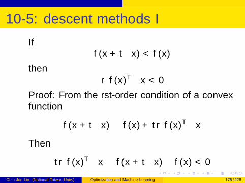
10-5: descent methods I
Iff (x + t∆x) < f (x)
then∇f (x)T∆x < 0
Proof: From the first-order condition of a convexfunction
f (x + t∆x) ≥ f (x) + t∇f (x)T∆x
Then
t∇f (x)T∆x ≤ f (x + t∆x)− f (x) < 0
Chih-Jen Lin (National Taiwan Univ.) Optimization and Machine Learning 175 / 228
10-6: line search types I
Why
α ∈ (0,1
2)?
The use of 1/2 is for convergence though we won’tdiscuss details
Finite termination of backtracking line search. Weargue that ∃t∗ > 0 such that
f (x + t∆x) < f (x) + αt∇f (x)T∆x ,∀t ∈ (0, t∗)
Otherwise,∃{tk} → 0
Chih-Jen Lin (National Taiwan Univ.) Optimization and Machine Learning 176 / 228
10-6: line search types II
such that
f (x + tk∆x) ≥ f (x) + αtk∇f (x)T∆x ,∀k
limtk→0
f (x + tk∆x)− f (x)
tk=∇f (x)T∆x ≥ α∇f (x)T∆x
However,
∇f (x)T∆x < 0 and α ∈ (0, 1)
cause a contradiction
Chih-Jen Lin (National Taiwan Univ.) Optimization and Machine Learning 177 / 228
10-6: line search types III
Graphical interpretation: the tangent line passesthrough (0, f (x)), so the equation is
y − f (x)
t − 0= ∇f (x)T∆x
Because∇f (x)T∆x < 0,
we see that the line of
f (x) + αt∇f (x)T∆x
Chih-Jen Lin (National Taiwan Univ.) Optimization and Machine Learning 178 / 228
10-6: line search types IV
is above that of
f (x) + t∇f (x)T∆x
Chih-Jen Lin (National Taiwan Univ.) Optimization and Machine Learning 179 / 228
10-7 I
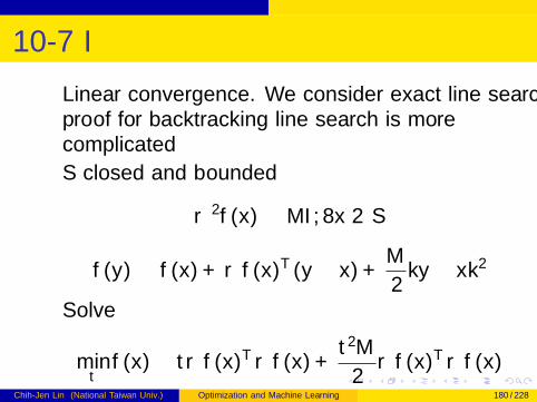
Linear convergence. We consider exact line search;proof for backtracking line search is morecomplicated
S closed and bounded
∇2f (x) � MI ,∀x ∈ S
f (y) ≤ f (x) +∇f (x)T (y − x) +M
2‖y − x‖2
Solve
mint
f (x)− t∇f (x)T∇f (x) +t2M
2∇f (x)T∇f (x)
Chih-Jen Lin (National Taiwan Univ.) Optimization and Machine Learning 180 / 228
10-7 II
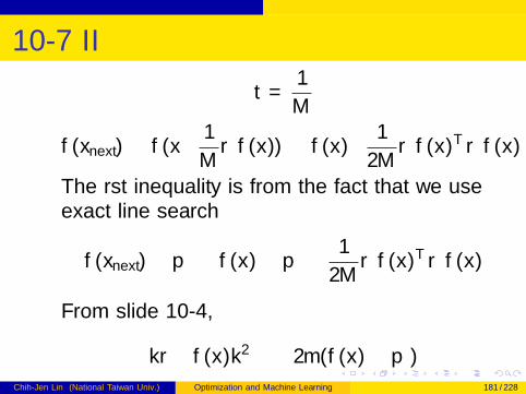
t =1
M
f (xnext) ≤ f (x− 1
M∇f (x)) ≤ f (x)− 1
2M∇f (x)T∇f (x)
The first inequality is from the fact that we useexact line search
f (xnext)− p∗ ≤ f (x)− p∗ − 1
2M∇f (x)T∇f (x)
From slide 10-4,
−‖∇f (x)‖2 ≤ −2m(f (x)− p∗)
Chih-Jen Lin (National Taiwan Univ.) Optimization and Machine Learning 181 / 228
10-7 III
Hence
f (xnext)− p∗ ≤ (1− m
M)(f (x)− p∗)
Chih-Jen Lin (National Taiwan Univ.) Optimization and Machine Learning 182 / 228
10-8 I
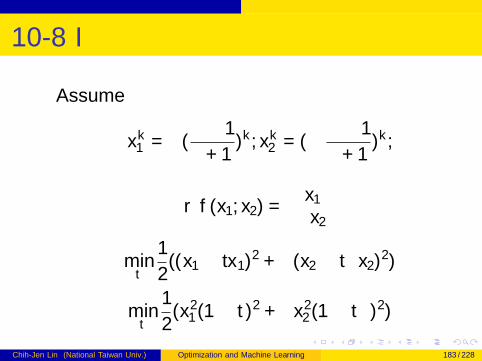
Assume
xk1 = γ(γ − 1
γ + 1)k , xk2 = (−γ − 1
γ + 1)k ,
∇f (x1, x2) =
[x1
γx2
]mint
1
2((x1 − tx1)2 + γ(x2 − tγx2)2)
mint
1
2(x2
1 (1− t)2 + γx22 (1− tγ)2)
Chih-Jen Lin (National Taiwan Univ.) Optimization and Machine Learning 183 / 228
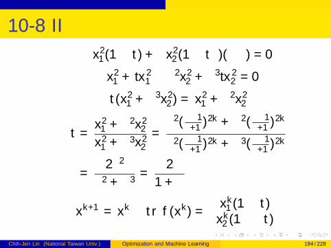
10-8 II
−x21 (1− t) + γx2
2 (1− tγ)(−γ) = 0
−x21 + tx2
1 − γ2x22 + γ3tx2
2 = 0
t(x21 + γ3x2
2 ) = x21 + γ2x2
2
t =x2
1 + γ2x22
x21 + γ3x2
2
=γ2(γ−1
γ+1)2k + γ2(γ−1γ+1)2k
γ2(γ−1γ+1)2k + γ3(γ−1
γ+1)2k
=2γ2
γ2 + γ3=
2
1 + γ
xk+1 = xk − t∇f (xk) =
[xk1 (1− t)xk2 (1− γt)
]Chih-Jen Lin (National Taiwan Univ.) Optimization and Machine Learning 184 / 228
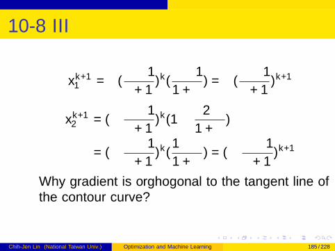
10-8 III
xk+11 = γ(
γ − 1
γ + 1)k(
γ − 1
1 + γ) = γ(
γ − 1
γ + 1)k+1
xk+12 = (−γ − 1
γ + 1)k(1− 2γ
1 + γ)
= (−γ − 1
γ + 1)k(
1− γ1 + γ
) = (−γ − 1
γ + 1)k+1
Why gradient is orghogonal to the tangent line ofthe contour curve?
Chih-Jen Lin (National Taiwan Univ.) Optimization and Machine Learning 185 / 228
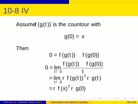
10-8 IV
Assume f (g(t)) is the countour with
g(0) = x
Then0 = f (g(t))− f (g(0))
0 = limt→0
f (g(t))− f (g(0))
t= lim
t→0∇f (g(t))T∇g(t)
=∇f (x)T∇g(0)
Chih-Jen Lin (National Taiwan Univ.) Optimization and Machine Learning 186 / 228
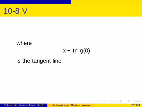
10-8 V
where
x + t∇g(0)
is the tangent line
Chih-Jen Lin (National Taiwan Univ.) Optimization and Machine Learning 187 / 228
10-10 I
linear convergence: from slide 10-7
f (xk)− p∗ ≤ ck(f (x0)− p∗)
log(ck(f (x0)− p∗)) = k log c + log(f (x0)− p∗)
is a straight line. Note that now k is the x-axis
Chih-Jen Lin (National Taiwan Univ.) Optimization and Machine Learning 188 / 228
10-11: steepest descent method I
(unnormalized) steepest descent direction:
∆xsd = ‖∇f (x)‖∗∆xnsd
Here ‖ · ‖∗ is the dual norm
We didn’t discuss much about dual norm, but wecan still explain some examples on 10-12
Chih-Jen Lin (National Taiwan Univ.) Optimization and Machine Learning 189 / 228
10-12 I
Euclidean: ∆xnsd is by solving
min ∇f Tvsubject to ‖v‖ = 1
∇f Tv = ‖∇f ‖‖v‖ cos θ = −‖∇f ‖ when cos θ = π
∆xnsd =−∇f (x)
‖∇f (x)‖‖∇f (x)‖∗ = ‖∇f (x)‖
‖∇f (x)‖∗∆xnsd = ‖∇f (x)‖∗−∇f (x)
‖∇f (x)‖= −∇f (x)
Chih-Jen Lin (National Taiwan Univ.) Optimization and Machine Learning 190 / 228
10-12 II
Quadratic norm: ∆xnsd is by solving
min ∇f Tvsubject to vTPv = 1
Now‖v‖P =
√vTPv ,
where P is symmetric positive definite
Chih-Jen Lin (National Taiwan Univ.) Optimization and Machine Learning 191 / 228
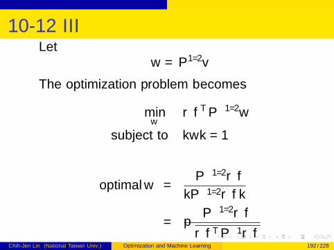
10-12 IIILet
w = P1/2v
The optimization problem becomes
minw
∇f TP−1/2w
subject to ‖w‖ = 1
optimal w =−P−1/2∇f‖P−1/2∇f ‖
=−P−1/2∇f√∇f TP−1∇f
Chih-Jen Lin (National Taiwan Univ.) Optimization and Machine Learning 192 / 228
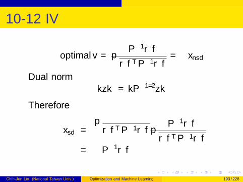
10-12 IV
optimal v =−P−1∇f√∇f TP−1∇f
= ∆xnsd
Dual norm‖z‖∗ = ‖P−1/2z‖
Therefore
∆xsd =√∇f TP−1∇f −P−1∇f√
∇f TP−1∇f= −P−1∇f
Chih-Jen Lin (National Taiwan Univ.) Optimization and Machine Learning 193 / 228
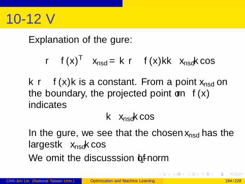
10-12 V
Explanation of the figure:
−∇f (x)T∆xnsd = ‖ − ∇f (x)‖‖∆xnsd‖ cos θ
‖ − ∇f (x)‖ is a constant. From a point ∆xnsd onthe boundary, the projected point on −∇f (x)indicates
‖∆xnsd‖ cos θ
In the figure, we see that the chosen ∆xnsd has thelargest ‖∆xnsd‖ cos θ
We omit the discusssion of l1-norm
Chih-Jen Lin (National Taiwan Univ.) Optimization and Machine Learning 194 / 228
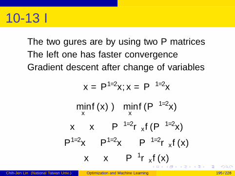
10-13 I
The two figures are by using two P matrices
The left one has faster convergence
Gradient descent after change of variables
x = P1/2x , x = P−1/2x
minx
f (x)⇒ minx
f (P−1/2x)
x ← x − αP−1/2∇x f (P−1/2x)
P1/2x ← P1/2x − αP−1/2∇x f (x)
x ← x − αP−1∇x f (x)
Chih-Jen Lin (National Taiwan Univ.) Optimization and Machine Learning 195 / 228

10-14 I
x
f ′(x)
Chih-Jen Lin (National Taiwan Univ.) Optimization and Machine Learning 196 / 228
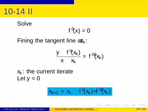
10-14 II
Solvef ′(x) = 0
Fining the tangent line at xk :
y − f ′(xk)
x − xk= f ′′(xk)
xk : the current iterateLet y = 0
xk+1 = xk − f ′(xk)/f ′′(xk)
Chih-Jen Lin (National Taiwan Univ.) Optimization and Machine Learning 197 / 228
10-16 I
f (y) = f (x) +∇f (x)T (y − x) +1
2(y − x)T∇2f (x)(y − x)
∇f (y) = 0 = ∇f (x) +∇2f (x)(y − x)
y − x = −∇2f (x)−1∇f (x)
infyf (y) = f (x)− 1
2∇f (x)T∇2f (x)−1∇f (x)
f (x)− infyf (y) =
1
2λ(x)2
Chih-Jen Lin (National Taiwan Univ.) Optimization and Machine Learning 198 / 228
10-16 II
Norm of the Newton step in the quadratic Hessian norm
∆xnt = −∇2f (x)−1∇f (x)
∆xTnt∇2f (x)∆xnt = ∇f (x)T∇2f (x)−1∇f (x) = λ(x)2
Directional derivative in the Newton direction
limt→0
f (x + t∆xnt)− f (x)
t=∇f (x)T∆xnt
=−∇f (x)T∇2f (x)−1∇f (x) = −λ(x)2
Chih-Jen Lin (National Taiwan Univ.) Optimization and Machine Learning 199 / 228
10-16 III
Affine invariant
f (y) ≡ f (Ty) = f (x)
Assume T is an invertable square matrix. Then
λ(y) = λ(Ty)
Proof:∇f (y) = TT∇f (Ty)
∇2f (y) = TT∇2f (Ty)T
Chih-Jen Lin (National Taiwan Univ.) Optimization and Machine Learning 200 / 228
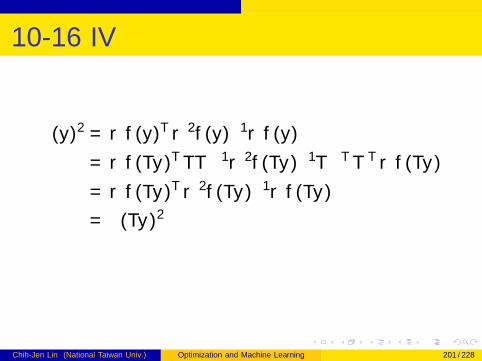
10-16 IV
λ(y)2 = ∇f (y)T∇2f (y)−1∇f (y)
= ∇f (Ty)TTT−1∇2f (Ty)−1T−TTT∇f (Ty)
= ∇f (Ty)T∇2f (Ty)−1∇f (Ty)
= λ(Ty)2
Chih-Jen Lin (National Taiwan Univ.) Optimization and Machine Learning 201 / 228
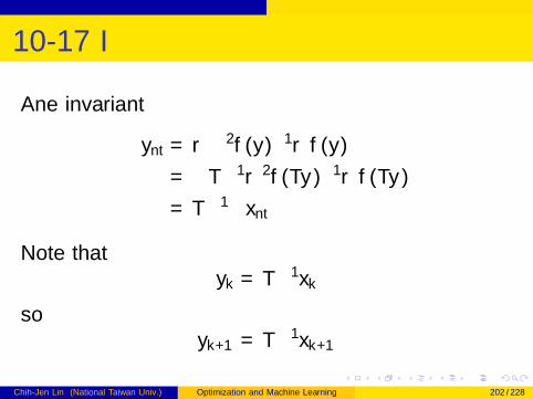
10-17 I
Affine invariant
∆ynt = −∇2f (y)−1∇f (y)
= −T−1∇2f (Ty)−1∇f (Ty)
= T−1∆xnt
Note thatyk = T−1xk
soyk+1 = T−1xk+1
Chih-Jen Lin (National Taiwan Univ.) Optimization and Machine Learning 202 / 228
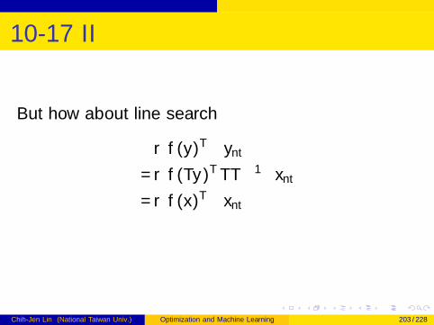
10-17 II
But how about line search
∇f (y)T∆ynt
=∇f (Ty)TTT−1∆xnt
=∇f (x)T∆xnt
Chih-Jen Lin (National Taiwan Univ.) Optimization and Machine Learning 203 / 228
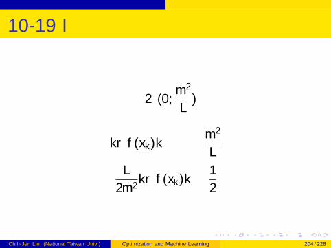
10-19 I
η ∈ (0,m2
L)
‖∇f (xk)‖ ≤ η ≤ m2
L
L
2m2‖∇f (xk)‖ ≤ 1
2
Chih-Jen Lin (National Taiwan Univ.) Optimization and Machine Learning 204 / 228
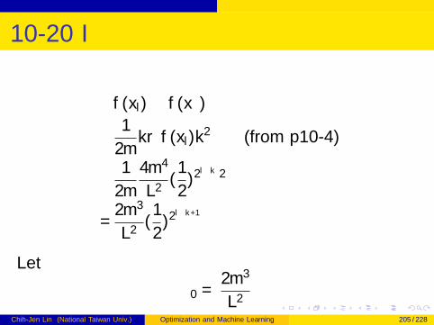
10-20 I
f (xl)− f (x∗)
≤ 1
2m‖∇f (xl)‖2 (from p10-4)
≤ 1
2m
4m4
L2(
1
2)2l−k ·2
=2m3
L2(
1
2)2l−k+1 ≤ ε
Let
ε0 =2m3
L2
Chih-Jen Lin (National Taiwan Univ.) Optimization and Machine Learning 205 / 228
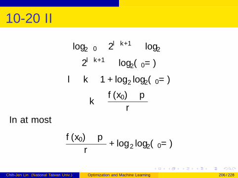
10-20 II
log2 ε0 − 2l−k+1 ≤ log2 ε
2l−k+1 ≥ log2(ε0/ε)
l ≥ k − 1 + log2 log2(ε0/ε)
k ≤ f (x0)− p∗
r
In at most
f (x0)− p∗
r+ log2 log2(ε0/ε)
Chih-Jen Lin (National Taiwan Univ.) Optimization and Machine Learning 206 / 228
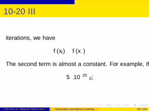
10-20 III
iterations, we have
f (xl)− f (x∗) ≤ ε
The second term is almost a constant. For example, if
ε ≈ 5 · 10−20ε0,
Chih-Jen Lin (National Taiwan Univ.) Optimization and Machine Learning 207 / 228
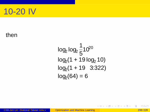
10-20 IV
then
log2 log2
1
51020
≈ log2(1 + 19 log2 10)
≈ log2(1 + 19 · 3.322)
≈ log2(64) = 6
Chih-Jen Lin (National Taiwan Univ.) Optimization and Machine Learning 208 / 228
10-22 I
On page 10-10, to reach
f (xk)− p∗ ≈ 10−4,
150 iterations are needed
However, the cost per Newton iteration may bemuch higher
Also for some applications we may not need a veryaccurate solution
Chih-Jen Lin (National Taiwan Univ.) Optimization and Machine Learning 209 / 228
10-29: implementation I
If H is positive definite, then there exists unique Lsuch that
H = LLT
λ(x) = (∇f (x)∇2f (x)−1∇f (x))1/2
= (gTL−TL−1g)1/2 = ‖L−1g‖2
Chih-Jen Lin (National Taiwan Univ.) Optimization and Machine Learning 210 / 228
10-30: example of dense Newton systemswith structure I
ψi(xi) : R → R
∇f (x) =
ψ′1(x1)...
ψ′n(xn)
+ AT∇ψ0(Ax + b)
Chih-Jen Lin (National Taiwan Univ.) Optimization and Machine Learning 211 / 228
10-30: example of dense Newton systemswith structure II
∇2f (x) =
ψ′′1 (x1). . .
ψ′′n(xn)
+ AT∇2ψ20(Ax + b)A
= D + ATH0A
H0 : p × p
method 2:∆x = D−1(−g − ATLow)
LT0 AD−1(−g − ATL0w) = w
Chih-Jen Lin (National Taiwan Univ.) Optimization and Machine Learning 212 / 228
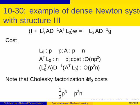
10-30: example of dense Newton systemswith structure III
(I + LT0 AD−1ATL0)w = −LT0 AD−1g
Cost
L0 : p × p,A : p × n
ATL0 : n × p, cost : O(np2)
(LT0 A)D−1(ATL0) : O(p2n)
Note that Cholesky factorization of H0 costs
1
3p3 ≤ p2n
Chih-Jen Lin (National Taiwan Univ.) Optimization and Machine Learning 213 / 228
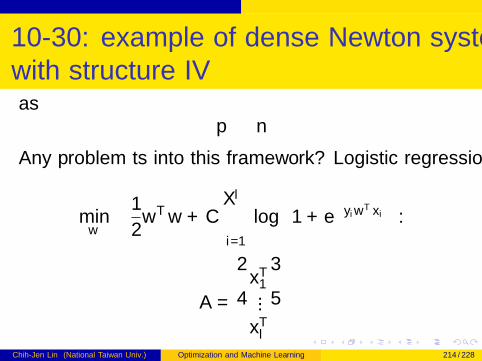
10-30: example of dense Newton systemswith structure IVas
p � n
Any problem fits into this framework? Logistic regression
minw
1
2wTw + C
l∑i=1
log(
1 + e−yiwTxi).
A =
xT1...xTl
Chih-Jen Lin (National Taiwan Univ.) Optimization and Machine Learning 214 / 228
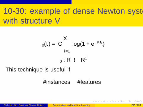
10-30: example of dense Newton systemswith structure V
ψ0(t) = Cl∑
i=1
log(1 + e−yi ti )
ψ0 : R l → R1
This technique is useful if
#instances� #features
Chih-Jen Lin (National Taiwan Univ.) Optimization and Machine Learning 215 / 228
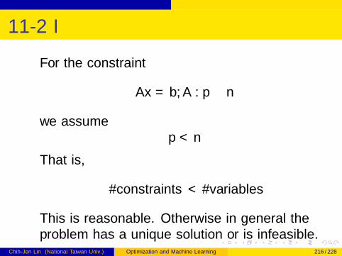
11-2 I
For the constraint
Ax = b,A : p × n
we assumep < n
That is,
#constraints < #variables
This is reasonable. Otherwise in general theproblem has a unique solution or is infeasible.
Chih-Jen Lin (National Taiwan Univ.) Optimization and Machine Learning 216 / 228
11-2 II
With p < n we can assume
rank(A) = p
Chih-Jen Lin (National Taiwan Univ.) Optimization and Machine Learning 217 / 228
11-3 I
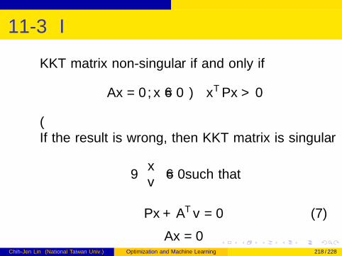
KKT matrix non-singular if and only if
Ax = 0, x 6= 0⇒ xTPx > 0
⇐If the result is wrong, then KKT matrix is singular
∃[xv
]6= 0such that
Px + ATv = 0 (7)
Ax = 0Chih-Jen Lin (National Taiwan Univ.) Optimization and Machine Learning 218 / 228
11-3 II
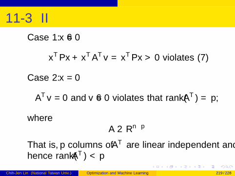
Case 1: x 6= 0
xTPx + xTATv = xTPx > 0 violates (7)
Case 2: x = 0
ATv = 0 and v 6= 0 violates that rank(AT ) = p,
whereA ∈ Rn×p
That is, p columns of AT are linear independent andhence rank(AT ) < p
Chih-Jen Lin (National Taiwan Univ.) Optimization and Machine Learning 219 / 228
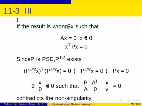
11-3 III⇒If the result is wrong, ∃x such that
Ax = 0, x 6= 0
xTPx = 0
Since P is PSD, P1/2 exists
(P1/2x)T (P1/2x) = 0⇒ P1/2x = 0⇒ Px = 0
∃[x0
]6= 0 such that
[P AT
A 0
] [xv
]= 0
contradicts the non-singularityChih-Jen Lin (National Taiwan Univ.) Optimization and Machine Learning 220 / 228
11-3 IV
KKT matrix non-singular if and only if
P + ATA � 0
⇐If the result is wrong, the matrix is singular. That
is, it does not have full rank. Thus, ∃[xv
]6= 0 such
thatPx + ATv = 0,Ax = 0
We claim thatx 6= 0
Chih-Jen Lin (National Taiwan Univ.) Optimization and Machine Learning 221 / 228
11-3 VOtherwise,
x = 0, v 6= 0
imply thatATv = 0,
a contradiction to
rank(AT ) = p
That is, columns of AT ’s p columns becomelinlinear dependent. Then
xT (P + ATA)x = xT (−ATv) = −(Ax)Tv = 0
Chih-Jen Lin (National Taiwan Univ.) Optimization and Machine Learning 222 / 228
11-3 VIleads to a contradiction⇒If
P + ATA � 0
∃x 6= 0 such that xTPx + xTATAx ≤ 0
Because
P + ATA is symmetric positive semi-definite,
we have
∃x 6= 0 such that xTPx + xTATAx = 0Chih-Jen Lin (National Taiwan Univ.) Optimization and Machine Learning 223 / 228
11-3 VIIBecause P and ATA are both PSD,
Ax = 0, xTPx = 0
Then [x0
]6= 0
is a solution of [P AT
A 0
] [xv
]= 0,
a contradiction
Chih-Jen Lin (National Taiwan Univ.) Optimization and Machine Learning 224 / 228
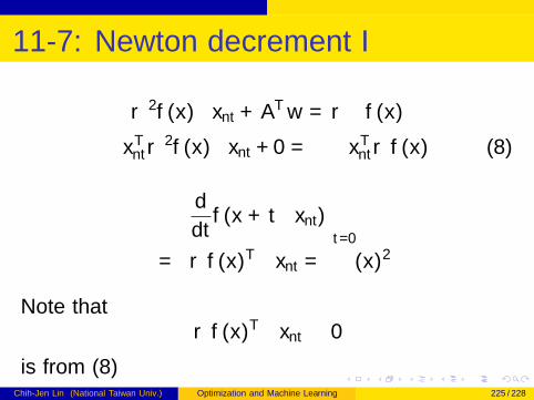
11-7: Newton decrement I
∇2f (x)∆xnt + ATw = −∇f (x)
∆xTnt∇2f (x)∆xnt + 0 = −∆xTnt∇f (x) (8)
d
dtf (x + t∆xnt)
∣∣∣∣t=0
= ∇f (x)T∆xnt = −λ(x)2
Note that∇f (x)T∆xnt ≤ 0
is from (8)Chih-Jen Lin (National Taiwan Univ.) Optimization and Machine Learning 225 / 228
11-8 I
Original
min f (x)
subject to Ax = b
Letx = Ty
New
miny
f (Ty) = f (y)
subject to ATy = b = Ay ,
Chih-Jen Lin (National Taiwan Univ.) Optimization and Machine Learning 226 / 228
11-8 II
whereA = AT
KKT system of the original one[∇2f (x) AT
A 0
] [vw
]=
[−∇f (x)
0
]New system[
∇2f (y) AT
A 0
] [vw
]=
[−∇f (y)
0
]Chih-Jen Lin (National Taiwan Univ.) Optimization and Machine Learning 227 / 228
11-8 III[TT∇2f (Ty)T TTAT
AT 0
] [vw
]=
[−TT∇f (Ty)
0
]If
x = Ty ⇒ v = T−1v , w = w is a solution
Let’s omit the step size
y ← y + v
Ty ← Ty + T v
v = T v
x ← x + v
Thus invariantChih-Jen Lin (National Taiwan Univ.) Optimization and Machine Learning 228 / 228
![Introduction to Symbolic Logic [1em] [width=.5]squirrel€¦ · Two Problems: Problem 1 This de nition of the valuation function has at least two problems: Problem 1: the valuation](https://static.fdocument.org/doc/165x107/5f0d9a7c7e708231d43b2c5a/introduction-to-symbolic-logic-1em-width5-two-problems-problem-1-this-de.jpg)