Dipartimento di Informatica eScienze dell’Informazione

Institut de Mathematiques de Luminy

••••• ••

λ-theories: some investigations

by

Luca Paolini

Theses Series DISI-TH-2003-XX

DISI, Universita di Genova IML, Universite de la MediterraneeV. Dodecaneso 35, 16146 Genova, Italy Campus de Luminy, 13288 Marseille, France

Universita degli Studi di GenovaUniversite de la Mediterranee

Dipartimento di Informatica e Scienze dell’Informazione

Institut de Mathematiques de Luminy

Dottorato di Ricerca in Informatica

Doctorat en Mathematiques Discretes et Fondements de l’Informatique

Ph.D. Thesis

λ-theories: some investigations

by

Luca Paolini

December, 2003

Dottorato di Ricerca in InformaticaDISI, Universita degli Studi di Genova

via Dodecaneso 3516146 Genova, Italy

Doctorat en Mathematiques Discretes et Fondements de l’InformatiqueIML, Universite de la Mediterranee

UPR 9016 Campus de Luminy, Case 90713288 Marseille Cedex 9, France

Ph.D. Thesis

Submitted by Luca Paolinipaolini@disi.unige.it,paolini@iml.univ-mrs.fr

Date of submission: November 2003

Title: λ-theories: some investigations

Advisors:J.Y. Girard G. RosoliniIML - UPR 9016 - CNRS DISI, Universita di Genovagirard@iml.univ-mrs.fr rosolini@disi.unige.it

Ext. Reviewers:A. Bucciarelli S. Ronchi Della RoccaPPS, Universite de Paris 7 DI, Universita di TorinoAntonio.Bucciarelli@pps.jussieu.fr ronchi@di.unito.it

Abstract

In this thesis we present somes investigations on λ-calculi, both untyped and typed. The first twoparts concerning some pure untyped calculi, while the last concerns PCF and an extension of itssyntax.

In the first part, a λ-calculus is defined, which is parametric with respect to a set ∆ of inputvalues and subsumes all the different (pure and untyped) λ-calculi given in the literature, inparticular the classical one and the call-by-value λ-calculus of Plotkin. It is proved that it enjoysthe confluence property, and a necessary and sufficient condition is given, under which it enjoysthe standardization property.

Hence, we extended some basic syntactical notion of the classical λ-calculus to the parametricλ∆-calculus such as solvability, separability, theory. We have studied the notions of solvabilityand separability in the call-by-value setting; unfortunately, there is no evidence on how treat thiskind of notions in an unified way for our parametric λ∆-calculus. On the other hand, we are ableto show that some property on theories hold for each λ∆-calculus.

The notion of solvability in the call-by-value λ-calculus has been defined and completely charac-terized, after the preliminary characterization of the class of potentially valuable terms. It turnsout that the call-by-value reduction rule (the βv-reduction of Plotkin) is too weak for capturingthe solvability property of terms, so some new reduction has been defined in order to do this.The notion of separability is the key notion used in the Bohm Theorem, proving that syntacticallydifferent βη-normal forms are separable in the classical λ-calculus endowed with β-reduction, i.e.in the call-by-name setting. In the case of call-by-value λ-calculus endowed with βv-reductionand ηv-reduction, it turns out that two syntactically different βη-normal forms are separable too,while the notions of βv-normal form and ηv-normal form are semantically meaningless.

In the second part, the semantics of the parametric λ∆-calculus is considered.A universal operational semantics is given through a reduction machine, parametric with respectto both ∆ and a set Θ of output values. It is showed that they can be instantiated in orderto give the more interesting operational reduction machines of untyped λ-calculi. This kindof operational semantics induces theories correct for the related λ∆-calculus. We study someproperty of the main instances of ∆ and Θ. We have defined some parametric notion, as thatof relevant contexts, operational extensionality and head-discriminability, hence we try to findsome general characterization.

It is showed that the standard operational equivalence induced from the Plotkin’s call-by-valueλ-calculus is not semisensible, namely there there is a solvable term equated to an unsolvableone.

Hence, a syntactical kind of model, said λ∆-interaction model is defined and showed to be fullyabstract for the main interesting universal operational semantics. This kind of model is built byintroducing the key notion of orthogonality, similar to that used in the Girard’s phase semanticsand ludics. By mimicking in an awful manner the Girard work, our notion of orthogonalityopposes λ-terms to contexts.Furthermore, we have showed a partial characterization of the orthogonality induced from theevaluation of terms to head normal form, in the classical call-by-name λ-calculus.

In the last part, we have studied a typed λ-calculus with constants (PCF -like) and its standardinterpretation on coherent spaces and stable functions. It is well-know that the model is not fullyabstract with respect to the standard operational semantics, since the Scott-continuous Gustavefunction. We have showed that in coherent spaces there is some stable function that is not Scott-continuous already in finite domains, thus these functions are independent from that of Gustavethat is continuous.Hence, we have extended both the syntax and the operational semantics of the considered lan-guage and we have showed that the interpretation of the extended language becomes fully ab-stract with respect to the standard interpretation on coherent spaces. Thus an operational charac-terization of stable functions (having domain/codomain on coherent spaces being interpretationon types of the language) is given.

After we have developped the results of this part of the thesis, we have discovered that the sameproblem was considered first by Jim and Meyer, on dI-domains. They have showed some neg-ative results. First they define in a denotational way some stable non-Scott-continuous functionsimilar to our one, hence they show that this operator break-down the coincidence between theapplicative-preorder on terms and the contextual-preorder. Finally, they show that with theirhuge class of “linear ground operational rules” defining some PCF -like rules of evaluation, thebefore considered coincidence, cannot be break-down. So they conclude that it is hard to findan extension of PCF endowed with operators having a meaningful operational desciption beingfully abstract with respect to stable functions.Although, one of the operators that we add to PCF fall down from their PCF -like rules, wethink that its meaning is rather clear.

A mio padre ed a tutta la mia famiglia.

Questo libro contiene almeno un errore. Ci si potrebbe aspettare che per verificarela cosa sia necessario leggere l’intero volume. E invece lo sappiamo gia fin d’ora.Infatti, se ci sono errori, ci sono. E se non ce ne sono, c’e quello che dice che questolibro contiene almeno un errore. Dunque sappiamo che in questo libro l’errore c’e,anche se non sappiamo ancora qual’e. (Piergiorgio Odifreddi)

Ringraziamenti

Ringrazio tutti coloro che in questi anni mi hanno aiutato e sostenuto,

... ... ...

Contents

I Parametric Syntax 1Introduction . . . . . . . . . . . . . . . . . . . . . . . . . . . . . . . . . . . . . . . . 2

Chapter 1 The parametric λ-calculus 6

1.1 The language of λ-terms . . . . . . . . . . . . . . . . . . . . . . . . . . . . . . 6

1.2 The λ∆-calculus . . . . . . . . . . . . . . . . . . . . . . . . . . . . . . . . . . . 9

1.2.1 Proof of Confluence and Standardization Theorems . . . . . . . . . . . . 18

1.2.2 Technical Remarks . . . . . . . . . . . . . . . . . . . . . . . . . . . . . 27

1.3 ∆-theories . . . . . . . . . . . . . . . . . . . . . . . . . . . . . . . . . . . . . . 30

1.3.1 ∆-pretheories . . . . . . . . . . . . . . . . . . . . . . . . . . . . . . . . 32

Chapter 2 The call-by-name λ-calculus 35

2.1 The syntax of λΛ-calculus . . . . . . . . . . . . . . . . . . . . . . . . . . . . . 35

2.1.1 Proof of Λ-solvability Theorem . . . . . . . . . . . . . . . . . . . . . . 38

2.1.2 Proof of Bohm’s Theorem . . . . . . . . . . . . . . . . . . . . . . . . . 39

Chapter 3 The call-by-value λ-calculus 46

3.1 The Syntax of the λΓ-calculus . . . . . . . . . . . . . . . . . . . . . . . . . . . 46

3.1.1 Ξ`-confluence and Ξ`-Standardization . . . . . . . . . . . . . . . . . . . 53

3.1.2 Proof of Potential Γ-valuability and Γ-solvability Theorems . . . . . . . 56

3.1.3 Proof of Γ-Separability Theorem . . . . . . . . . . . . . . . . . . . . . . 63

3.2 Potential Valuability and Λ-reduction . . . . . . . . . . . . . . . . . . . . . . . 72

I

II Parametric Semantics 74Introduction . . . . . . . . . . . . . . . . . . . . . . . . . . . . . . . . . . . . . . . . 75

Chapter 4 Parametric Operational Semantics 78

4.1 The universal ∆-reduction machine . . . . . . . . . . . . . . . . . . . . . . . . . 84

4.1.1 Set of Input and Output Valuable Terms . . . . . . . . . . . . . . . . . . 87

Chapter 5 Call-by-name operational semantics 90

5.1 H-operational semantics . . . . . . . . . . . . . . . . . . . . . . . . . . . . . . 90

5.2 N-operational semantics . . . . . . . . . . . . . . . . . . . . . . . . . . . . . . 95

5.3 L-operational semantics . . . . . . . . . . . . . . . . . . . . . . . . . . . . . . . 99

5.3.1 An example . . . . . . . . . . . . . . . . . . . . . . . . . . . . . . . . . 103

Chapter 6 Call-by-value operational semantics 108

6.1 V-operational semantics . . . . . . . . . . . . . . . . . . . . . . . . . . . . . . 108

6.1.1 An example . . . . . . . . . . . . . . . . . . . . . . . . . . . . . . . . . 112

Chapter 7 Operational Theories 115

7.1 Operational semantics and extensionality . . . . . . . . . . . . . . . . . . . . . 115

7.2 Head-discriminability . . . . . . . . . . . . . . . . . . . . . . . . . . . . . . . . 120

7.2.1 H is head-discriminable . . . . . . . . . . . . . . . . . . . . . . . . . . 121

7.2.2 N is head-discriminable . . . . . . . . . . . . . . . . . . . . . . . . . . 122

7.2.3 L is head-discriminable . . . . . . . . . . . . . . . . . . . . . . . . . . . 123

7.2.4 V is head-discriminable . . . . . . . . . . . . . . . . . . . . . . . . . . 124

Chapter 8 λ∆-Interaction Models 126

8.1 Orthogonality . . . . . . . . . . . . . . . . . . . . . . . . . . . . . . . . . . . . 130

8.2 Union and Intersection . . . . . . . . . . . . . . . . . . . . . . . . . . . . . . . 133

8.2.1 Orthogonal Lattices . . . . . . . . . . . . . . . . . . . . . . . . . . . . . 134

8.3 Set applications . . . . . . . . . . . . . . . . . . . . . . . . . . . . . . . . . . . 135

II

8.4 λ∆-interaction models . . . . . . . . . . . . . . . . . . . . . . . . . . . . . . . . 137

8.5 Some further operations . . . . . . . . . . . . . . . . . . . . . . . . . . . . . . . 140

8.6 The λΛ-interaction modelH . . . . . . . . . . . . . . . . . . . . . . . . . . . . 142

8.6.1 Proof of Semi-separability . . . . . . . . . . . . . . . . . . . . . . . . . 147

III A Typed calculus 151Introduction . . . . . . . . . . . . . . . . . . . . . . . . . . . . . . . . . . . . . . . . 152

Chapter 9 Stable PCF 155

9.1 Syntax of PCF . . . . . . . . . . . . . . . . . . . . . . . . . . . . . . . . . . . 155

9.2 Mathematical Preliminaries . . . . . . . . . . . . . . . . . . . . . . . . . . . . . 161

9.3 Coherent Spaces . . . . . . . . . . . . . . . . . . . . . . . . . . . . . . . . . . . 164

9.4 Interpretation of PCF . . . . . . . . . . . . . . . . . . . . . . . . . . . . . . . 167

9.5 Correctness of PCF . . . . . . . . . . . . . . . . . . . . . . . . . . . . . . . . 173

9.5.1 Some Examples . . . . . . . . . . . . . . . . . . . . . . . . . . . . . . . 175

9.5.2 Parallel-If and Gustave Function . . . . . . . . . . . . . . . . . . . . . . 177

9.5.3 Another Gap . . . . . . . . . . . . . . . . . . . . . . . . . . . . . . . . 178

9.5.4 Non-Scott-Continuous Stable Functions . . . . . . . . . . . . . . . . . . 178

9.6 Syntax of StPCF . . . . . . . . . . . . . . . . . . . . . . . . . . . . . . . . . . 179

9.6.1 Structured Operational Semantics . . . . . . . . . . . . . . . . . . . . . 182

9.7 Interpretation of StPCF . . . . . . . . . . . . . . . . . . . . . . . . . . . . . . 192

9.8 Correctness of StPCF . . . . . . . . . . . . . . . . . . . . . . . . . . . . . . . 198

9.9 Definability and Full Abstraction of StPCF . . . . . . . . . . . . . . . . . . . . 199

Bibliography 207

Index 214

III

Part I

Parametric Syntax

1

I. Introduction

The λ-calculus, in its different variants, has been used as paradigmatic language for studyingvarious properties of programming languages [60, 61, 67, 78, 103]. In particular, the classicalλβ-calculus [4, 6, 18, 58, 90] and the λβv-calculus of Plotkin [81, 50] are paradigms for two dif-ferent parameter passing policies, the call-by-name and the call-by-value respectively. Althoughthe lexicon of both languages is the same, the reduction rule of λβv-calculus is obtained as arestriction of the classical β-rule. Thus, these two λ-calculi appear different both from syntacticand semantic point of view: in fact they have been studied using different tools [2, 6, 7, 32].

We propose a new λ-calculus, the λ∆-calculus, which is parametric with respect to a subset ∆

of terms that we call input values. The λ∆-calculus is a call-by-value calculus, in the sense thatthe reduction rule is a kind of conditioned β-rule, firing just in case the argument belong to ∆.Informally, input values represent partially evaluated terms, that can be passed as parameters.The only conditions we ask on the set ∆ is to be closed under substitution and reduction: theseconditions are quite natural, in order to preserve the status of an input, during the computation.

The λ∆-calculus subsumes a plethora of different variants of calculi, including both λβ and λβv

calculi. The λβ-calculus is obtained by putting ∆ = Λ, while λβv-calculus by putting ∆ =

Var ∪ λx.M | M ∈ Λ, i.e., variables and abstractions. Moreover it can suggest new kinds ofcalculi: in particular, we can easily prove that calculi already studied, as the calculus obtained bychoosing as input values the set Var∪M | M is a closed β-normal-form , enjoy good properties.

The idea of a parametric λ-calculus has been already introduced in [88], and has been usedfor defining a new parametric notion of extensionality, related to operational semantics. Theparametric λ-calculus is the skeleton on which [89] has been developed. An interesting uniformapproach to call-by-name and call-by-value computations, in a typed setting, has been presentedin [23], using a language derived from Gentzen’s sequence calculus LK.

The interest of such a new λ-calculus is that it is a setting where different λ-calculi can be studiedin an uniform manner. As a first example, we explore the conditions on the set of input valuesthat guarantee confluence property and standardization property, which are two basic propertieswe expect for a sequential programming language.

Confluence assures us that, when the result of a computation exists, it is unique; we prove that,for every choice of input values, the λ∆-calculus enjoys this property.

The standardization property says that every reduction sequence can be “sequentialized” in agiven order. At a first sight it’s difficult to deal with the standardization in a uniform manner.Both λβ and λβv calculi enjoy standardization, but in the first calculus a reduction when redexesare reduced from left to right is always standard, while in the second one the order is very tricky,see [81] and [73].

2

For example, let us consider the term M ≡ (λx.xx)(II), where I ≡ λx.x.Clearly M reduces to I in both λβ and λβv calculi, but in λβ-calculus the standard reductionsequence is (λx.xx)(II) →β II(II) →β I(II) →β II →β I, while in λβv-calculus the standardreduction sequence is (λx.xx)(II)→βv (λx.xx)I →βv II →βv I.

We give a notion of “sequentialization” that subsumes both cases, and we state a necessary andsufficient condition on the set of input values that assures the standardization property.

In the literature about λ-calculus, two notions of standardization have been defined, the classicalone [6], and a “strong” one, [57]. According to the former, a given reduction sequence canbe standardized in more than one way, while, according to the latter, there is just one standardreduction sequence corresponding to a given one. We choose this second approach.

We prove that the restriction to closed terms of theories induced by the λ∆-calculi determineuniquely their extension to all terms. This property will be quite useful in the second part of thethesis, where some kind of semantics will be introduced.

Not all the key properties of λ-calculus can be easily studied in an uniform manner using as toolthe λ∆-calculus. As example, we show that the notion of solvability is quite different in λβ andin λβv settings. The definition is uniform, since a term is solvable if and only if it can reduceto the identity, when applied to suitable arguments [6, 58]. But in the classical λβ-calculus thisnotion corresponds to an operational property of terms; being solvable all and only the terms thatreduce to head normal form, while in λβv the solvability cannot be expressed in the same way[73, 76].

In fact there are βv-normal forms which are unsolvable, as for example the term:

λx.(λy.∆)(xI)∆ which is operationally equivalent to λx.∆∆.

So, in order to characterize the call-by-value solvability, a more refined tool must be designed.To do so, we extend the notion of valuability (namely reducibility to values) to open terms, bydefining a term M being potentially valuable if and only if there is a substitution s, replacingvariables by closed values, such that s(M) is valuable. It turns out that the class of the call-by-value solvable terms is properly contained in that one of the potentially valuable terms. We willshow that the potentially valuable terms are completely characterized through a reduction →Ξ`

performing the classical β-reduction according to the innermost-lazy strategy. Hence, the call-by-value solvability has been characterized by a reduction extending recursively the reduction→Ξ` on subterms.It turns out that a term M is v-solvable if and only if it-reduces to a term of the shape:

λx1. . .xn.xiP1. . .Pm

where each Pi is potentially valuable (1 ≤ i ≤ m). Unfortunately this definition cannot beexpressed through the βv-reduction.

3

Another properties of λ-calculus that we have not be able to study in a uniform manner using astool the λ∆-calculus is the separability [13, 14].

The classical call-by-name notion of separability is: “two terms M,N are separable if and only ifthere exists a context C[.], such that C[M] =β x and C[N] =β y, where x, y are different variables”(see [6]). The Bohm Theorem says that two different βη-normal forms are separable.

The importance of Bohm Theorem has been pointed out by Wadsworth, which in [102] says:“The Church-Rosser Theorem shows that distinct normal forms cannot be proved equals bythe conversion rules; the Bohm Theorem shows that if one were ever to postulate, as an extraaxiom, the equality of two distinct normal forms, the resulting system would be inconsistent”.Note that the Bohm Theorem allows the coding of computable functions in λ-calculus, sinceby representing different natural numbers by different βη-normal forms, assures us that theirrepresentations is different in every consistent λ-theory [6, 75].

We have studied the separability in the particular setting of the call-by-value λ-calculus. It isnatural, to state that two terms M,N are v-separable if and only if there exists a context C[.],such that C[M] =βv x and C[N] =βv y, where x, y are different variables.

Thus, the naıve adaptation of Bohm-Theorem to call-by-value λ-calculus would be:

“two different βvηv-normal forms are v-separable”.

It is immediate to check that two syntactically different βvηv-normal forms are not always sepa-rable, for example consider the following terms: λx.xxx and λx.(λz.xxx)(xx). Thus, βvηv-normalforms are not semantically meaningful.

The right property in the call-by-value setting [75] is:

“two different βη-normal forms are v-separable”.

This separation result is based on the fact that every subterm of a βη-normal form is a potentiallyvaluable term.

Actually a sort of separation completeness holds, namely for each M ∈ Λ there is N ∈ βη-normalform such that, for all C[.],

• C[M]→βv x implies C[N]→βv x;

• C[N]→βv x implies, either C[M]→βv x or C[M] is not valuable.

A main difficulty in carrying out the proof of Bohm-Theorem, basically consists in handling opensubterms that are neither values nor valuables (because they are in normal form). For instance,

4

let M ≡ x(xP0)Q and N ≡ x(xP1)Q be βη-normal forms. A context C[.] v-separating M and Nneed to handle subterms as xP0, xP1 and Q by using the βv-reduction. Thus, C[.] needs beingable to transform xP0, xP1 and Q in values, by a “uniform substitution” preserving the structuraldifference. We show as it is possible to build such a substitution.The separation property will be proved by giving an algorithm separating β-normal forms, thussome β-reduction is taken in order to normalize terms after substitutions; hence, an additionalproblem is to show that these β-reductions can be “reconciled”, in some sense, with βv-reductions.Since from =β*=βv follows that separation results using β-reduction as computation rule do notimply the v-separation results.

A theory of call-by-value λ-calculus is a congruence relation, containing the relation =βv .Let =T be a such theory; if M and N are v-separable terms, such that M =T N then =T isinconsistent, i.e. all terms are equals. In fact, if C[.] is the context such that C[M] =βv xand C[N] =βv y then P =βv (λxy.C[M])PQ =βv (λxy.C[N])PQ =βv Q, for every P,Q ∈ Λ.Therefore, the semantical consequence of the separability result, is that two different βη-normalforms cannot be equated in consistent theories of call-by-value λ-calculus.

Last, some interesting relation between call-by-value potentially valuable terms and call-by-name lazy strongly normalizing terms is showed.

5

Chapter 1

The parametric λ-calculus

A calculus is a language equipped with some reduction rules. The calculi we will consider inthis part of the thesis share the same language, which is the language of λ-calculus, while theydiffer each other in their reduction rules.In order to treat them in an uniform way we define a parametric calculus, the λ∆-calculus, whichgive rise to different calculi by different instantiations of the parameter ∆. This part is devotedto study the syntactical properties of the λ∆-calculus, and in particular of its two most importantinstances, the call-by-name and the call-by-value λ-calculus.

1.1 The language of λ-terms

Definition 1.1.1 (The language Λ)Let Var be a countable set of variables. The set Λ of λ-terms is a set of words on the alphabetVar ∪ ((( , ))) , ... , λ inductively defined as follows:

• x ∈ Var implies x ∈ Λ (variable);

• M ∈ Λ and x ∈ Var implies (λx.M) ∈ Λ (abstraction);

• M ∈ Λ and N ∈ Λ implies (MN) ∈ Λ (application).

λ-terms will be ranged over by latin capital letters. Sets of λ-terms will be denoted by greekcapital letters.

Sometimes, we will refer to λ-terms simply as terms. The symbol ≡ will denote syntacticalidentity of terms.

6

We will use the following abbreviations, in order to avoid an excessive number of parenthesis:λx1...xn.M will stand for (λx1(...(λxn.M)...)) and MN1N2...Nn will stand for (...((MN1)N2)...Nn).Moreover ~M will denote a sequence of terms M1,. . .,Mn, for some n ≥ 0, and λ~x.M and ~M ~N,will denote respectively λx1. . .xn.M and M1. . .MmN1. . .Nn, for some n,m ≥ 0. The length of thesequence ~N is denoted by ‖~N‖.

Example 1.1.2 Some λ-terms have standard names, for historical reasons. A list of names thatwill be extensively used in this thesis is:

I ≡ λx.x,K ≡ λxy.x,O ≡ λxy.y,D ≡ λx.xx, E ≡ λxy.xy.

Definition 1.1.3 (Subterms)A term N is a subterm of M if and only if one of the following conditions arises:

• M ≡ N;

• M ≡ λx.M′ and N is a subterm of M′;

• M ≡ PQ and N is a subterm either of P or of Q.

A term N occurs in a term M if and only if N is a subterm of M.

The symbol λ plays the role of binder for variables, as formalized in the next definition.

Definition 1.1.4 (Free variables) i) The set of free variables of a term M, denoted by FV(M),is inductively defined as follows:

• M ≡ x implies FV(M) = x;• M ≡ λx.M′ implies FV(M) = FV(M′) − x;• M ≡ PQ implies FV(M) = FV(P) ∪ FV(Q).

A variable is bound in M if it is not free in M.

ii) A term M is closed if and only if FV(M) = ∅. A term is open if it is not closed. For everysubset of terms Θ ⊆ Λ, we will denote with Θ0 the restriction of Θ to closed terms.

The replacement of a free variable by a term is the basic syntactical operation on Λ, on whichthe definition of reduction rules will be based. But the replacement must respect the status of thevariables: e.g., x can be replaced by M ≡ λy.zy in λu.xu, so obtaining the term λu.(λy.zy)u, whilethe same replacement cannot take place in the term λz.xz, since in the obtained term λz.(λy.zy)zthe free occurrence of z in M would become bound. The notion is formalized in the next defini-tion.

7

Definition 1.1.5 The statement “M is free for x in N” is defined by induction on N as follows:

• M is free for x in x;

• M is free for x in y;

• if M is free for x both in P and Q then M is free for x in PQ;

• if M is free for x in N and x . y and y < FV(M)then M is free for x in λy.N.

Example 1.1.6 λxy.xz is free for x and y in (λu.x)(λu.xz), but is not free for u in both λxz.u andλzu.u.

Let M be free for x in N; thus N[M/x] denotes the simultaneous replacement of all free occur-rences of x in N by M. Clearly

FV(N[M/x]) =

FV(N) if x < FV(N)(FV(N) − x) ∪ FV(M) otherwise.

For example, (λx.u(xy))[xy/u] is not defined, because xy is not free for u in λx.u(xy), while(λx.u(xu))[u(λz.z)/u] ≡ λx.u(λz.z)(xu(λz.z)).

Both ~M[N1/x1, ...,Nn/xn] and ~M[~N/~x], where ‖~N‖ = ‖~x‖, are abbreviations for the simultaneousreplacement, in every M j, of xi by Ni (0 ≤ i ≤ ‖~x‖ = n, 0 ≤ j ≤ ‖ ~M‖).

In the standard mathematical notation, the name of a bound variable is meaningless: for example,∑1≤i≤n i and

∑1≤ j≤n j both denote the sum of the first n natural numbers. Also in the language Λ,

it is natural to consider the terms modulo names of bound variables. The renaming is formalizedin the next definition.

Definition 1.1.7 (α-reduction) i) λx.M →α λy.M[y/x] if y is free for x in M and y < FV(M).

ii) =α is the reflexive, symmetric, transitive and contextual closure of→α.

In all the thesis, we will consider terms modulo =α.

Thus we can safely extend the notation N[M/x] also to the case where M is not free for x in N.In this case N[M/x] denotes the result of replacing x by M in a term N ′ =α N such that M is freefor x in N′. Clearly such an N′ always exists and the notation is well posed. So (λx.u(xy))[xy/u]is α-equivalent to the term λz.xy(zy).

8

An alternative way of denoting a simultaneous replacement is by explicitly using the notionof substitution. A substitution is a function from variables to terms. If s is a substitution andFV(M) = x1, ..., xn, s(M) denotes M[s(x1)/x1, ..., s(xn)/xn].

An important syntactical tool that will be extensively used in the sequel is the notion of context.Informally, a context is a term that can contain some occurrences of a hole (denoted by theconstant [.]), that can be filled by a term.

Definition 1.1.8 (Context)Let Var be a countable set of variables, and [.] be a constant (the hole).

i) The set ΛC of contexts is a set of words on Var ∪ ((( , ))) , ... , λ , [.][.][.] inductively defined asfollows:

• [.] ∈ ΛC;

• x ∈ Var implies x ∈ ΛC;

• C[.] ∈ ΛC and x ∈ Var implies (λx.C[.]) ∈ ΛC;

• C1[.] ∈ ΛC and C2[.] ∈ ΛC implies (C1[.]C2[.]) ∈ ΛC.Contexts will be denoted by C[.],C′[.],C1[.]....

ii) A context of the shape: (λ~x.[.])~P is an head context.

iii) Let C[.] be a context and M be a term. Then C[M] denotes the term obtained by replacingby M every occurrence of [.] in C[.].

We will use for contexts the same abbreviate notations than for terms.

Note that filling a hole in a context is not a substitution; in fact free variables in M can becomebound in C[M]. For example, filling the hole of λx.[.] with the free variable x gives as result theterm λx.x.

1.2 The λ∆-calculus

We will present some λ-calculi, all based on the language Λ, defined in the previous section,each one characterized by different reduction rules.

The λ∆-calculus is the language Λ equipped with a set ∆ ⊆ Λ of input values, satisfying some clo-sure conditions. Informally, input values represent partially evaluated terms, that can be passed

9

as parameters. Call-by-name and call-by-value parameter passing can be seen as the two mostradical choices: parameters are not evaluated in the former policy, while in the latter they areevaluated until an output result is reached.

Most of the known variants of λ-calculus can be obtained from this parametric calculus by in-stantiating ∆ in a suitable way. The set ∆ of input values and the reduction →∆, induced by it,are defined in the next definition.

Definition 1.2.1 Let ∆ ⊆ Λ.

i) The ∆-reduction (→∆) is the contextual closure of the following rule:

(λx.M)N → M[N/x] if and only if N ∈ ∆.

(λx.M)N is called a ∆-redex (or simply redex) and M[N/x] is called its ∆-contractum (orsimply contractum).

ii) →∗∆

and =∆ are respectively the reflexive and transitive closure of →∆ and the symmetric,reflexive and transitive closure of→∆.

iii) A set ∆ ⊆ Λ is said set of input values, when the following conditions are satisfied:

• Var ⊆ ∆ (Var-closure);

• P,Q ∈ ∆ implies P[Q/x] ∈ ∆, for each x ∈ Var (substitution closure);

• M ∈ ∆ and M →∆ N imply N ∈ ∆ (reduction closure).

iv) A term is in ∆-normal form (∆-nf) if it has not ∆-redexes and it has a ∆-normal form, or it is∆-normalizing if it reduces to a ∆-normal form; the set of ∆-nf is denoted by ∆-NF.

v) A term is ∆-strongly normalizing if it is ∆-normalizing and moreover there is not an infinite∆-reduction sequence starting from it.

The closure conditions on the set of input values need some comment. Since, as already said,input values represent partially evaluated terms, it is natural to ask that this partial evaluation ispreserved by reduction, which is the rule on which is based the evaluation process. The substitu-tion closure comes naturally from the fact that variables always belong to the set of input values.

In all the thesis the symbol ∆ will denote a generic set of input values. We will omit the prefix ∆

in case it will be clear from the context.

10

Example 1.2.2 Let I,K,O,D the terms defined in the Example 1.1.2, and let M,N be inputvalues. Then IM →∆ M, so I has the behaviour of the identity function, KMN →∗

∆M, OMN →∗

∆

N, DM →∆ MM. If D ∈ ∆ then DD→∗∆

DD.

Now some possible sets of input values will be defined.

Definition 1.2.3 i) Γ = Var ∪ λx.M | M ∈ Λ;ii) ΛI is the language obtained from the grammar generating Λ, given in the Definition 1.1.1, by

modifying the formation rule for abstraction in the following way:

(λx.M) ∈ ΛI if and only if M ∈ Λ and x ∈ Var and x occurs in M.

The next property shows that there exists some set of input values, although not all set of termsare sets of input values.

Property 1.2.4 1. Λ is a set of input values;

2. Γ is a set of input values;

3. ΛI is a set of input values;

4. Λ-NF is not a set of input values;

5. Var ∪ Λ-NF0 is a set of input values;

6. Υ = Var ∪ λx.P | x ∈ FV(P) is not a set of input values.

Proof. The first case is obvious. In cases 2,3,5, it is easy to check that the closure properties ofDefinition 1.2.1 are satisfied. Λ-NF is not closed under substitution.It is easy to see that Υ is closed under substitution. But it is not closed under reduction. In factλx.KIx ∈ Υ, while λx.KIx→Υ λx.I < Υ.

The coice ∆ = Λ gives rise the classical call-by-name λ-calculus [18], while ∆ = Γ gives rise toa pure version (i.e., without constants) of the call-by-value λ-calculus, first defined by Plotkin[81].

The fact that Var ∪ Λ-NF0 is a correct set of input values has been first noticed in [29] and thenthe calculus has been studied in [50].

11

It is easy to check that every term M has the following shape:

λx1...xn.ζM1...Mm (n,m ≥ 0),

where Mi ∈ Λ are the arguments of M (1 ≤ i ≤ m) and ζ is the head of M. ζ is either a variable(head variable) or an application of the shape (λz.P)Q, which can be either a redex (head redex)or not (head block), depending on the fact that Q belong or not to the set ∆.

The natural interpretation of an abstraction term λx.M is a function whose formal parameter isx. The interpretation of an application (λx.M)N, when N ∈ ∆, is the application of the functionλx.M to the actual parameter N and so the ∆-reduction rule models the replacement of the formalparameter x by the actual parameter N in the body M of the function. Thus the ∆-normal formof a term, if it exists, can be seen as the final result of a computation.

The following fundamental theorem implies that this interpretation is correct, i.e. if the compu-tation process stops, then the result is unique.

Theorem 1.2.5 (Confluence) [77] Let M →∗∆

N1 and M →∗∆

N2.There is Q such that both N1 →∗∆ Q and N2 →∗∆ Q.

Proof. See subsection 1.2.1.

Corollary 1.2.6 The ∆-normal form of a term, if it exists, is unique.

Proof. Assume by absurdum that a term M has two different normal forms M1 and M2. Then,by the Confluence Theorem, there is a term N such that both M1 and M2 ∆-reduce to N, againstthe hypothesis that both are normal forms.

It is natural to ask if the closure conditions on input values, given in Definition 1.2.1, are neces-sary in order to assure the confluence of the calculus. It can be observed that they are not strictlynecessary, but a weaker version of them is needed. The question is considered in detail in thesubsection 1.2.2.

Assume M →∗∆

N; the Standardization Theorem says that, in case the set of input values enjoys aparticular property, there is a “standard” reduction sequence from M to N, reducing the redexesin a given order.

Let us introduce formally the notion of standard reduction sequence.

12

Definition 1.2.7

i) A symbol λ in a term M is active if and only if it is the first symbol of a ∆-redex of M.

ii) The ∆-sequentialization (M) of a term M is a function from Λ to Λ defined as follows:

• (xM1...Mm) = x(M1)...(Mm);

• ((λx.P)QM1...Mm) = (λx.P)(Q)(M1)...(Mm), if Q ∈ ∆;

• ((λx.P)QM1...Mm) = (Q)(λx.P)(M1)...(Mm), if Q < ∆;

• (λx.P) = λx.(P).

iii) The degree of a redex R in M is the numbers of λ’s which both are active in M and occur onthe left of (R) in (M).

iv) The principal redex of M, if it exists, is the redex of M with minimum degree.The principal reduction M →p

∆N denotes that N is obtained from M by reducing the

principal redex of M. →∗p∆

is the reflexive and transitive closure of→p∆.

v) A sequence M ≡ P0 →∆ P1 →∆ ... →∆ Pn →∆ N is standard if and only if the degree of theredex contracted in Pi is less than or equal to the degree of the redex contracted in Pi+1,for every i < n.We denote by M →

∆N a standard reduction sequence from M to N.

It is important to notice that the degree of a redex can change during the reduction, in partic-ular the redex of minimum degree has always degree zero. Moreover note that the reductionsequences of length 0 and 1 are always standard.

It is easy to check that, for every M, the Λ-sequentialization is (M) ≡ M; thus in this case theredex of degree 0 is always the leftmost one.

Example 1.2.8 1) Let ∆ = Λ, and let M ≡ (λx.x(KI))(II). Thus M has degree 0, KI has de-gree 1 and II has degree 2 (in the term M). The following reduction sequence is standard:(λx.x(KI))(II)→Λ (II)(KI)→Λ I(KI)→Λ I(λy.I).

2) Let M be as before, and let ∆ = Γ. Thus II has degree 0, and KI has degree 1. Note thatnow M is no more a redex. The following reduction sequence is standard: (λx.x(KI))(II)→Γ

(λx.x(KI))I →Γ I(KI)→Γ I(λy.I)→Γ λy.I.

3) Let M be as before, and let ∆ = Var ∪ Λ-NF0. Thus KI has degree 0 and II has degree1. Also in this case M is not a redex. The following reduction sequence is standard:(λx.x(KI))(II)→∆ (λx.x(KI))I →∆ (λx.x(λy.I))I.

13

The notion of a standard set of input values, which will be given in the next definition, is the keyone for having the standardization property.

Definition 1.2.9 (Standard Input Values) A set ∆ of input values is standard if and only if M <∆ and M →∗

∆N by reducing at every step a not principal redex imply N < ∆.

Now the standardization property can be stated.

Theorem 1.2.10 (Standardization) [77] Let ∆ be standard.M →∗

∆N implies there is a standard reduction sequence from M to N.

Proof. See subsection 1.2.1.

The next property shows that some set of input values is standard, while someone is not standard.

Property 1.2.11 i) Λ and Γ are standard;

ii) For every ∆, Var ∪ ∆-NF0 is standard;

iii) ΛI is not standard.

Proof.

i) Λ is trivially standard. Let us consider Γ; we will prove that, if M < Γ, and M →Γ N througha not principal reduction, then N < Γ.M < Γ implies that M has one of the following shapes:

1) yM1...Mm (m > 1);

2) (λx.M1)M2...Mm (m ≥ 2) and either (λx.M1)M2 is a redex or it is a head block.

Case 1 is trivial, since M can never be reduced to a term in Γ.In case 2, if M2 ∈ Γ then the principal redex is (λx.M1)M2, while if M2 < Γ then if M2 < Γ-NF the principal redex is in M2, if M2 ∈ Γ-NF then the principal redex is in some M j

( j ≤ 3). So the reduction of a not principal redex cannot produce a term belonging to Γ.

ii) Var ∪ ∆-NF0 is standard since not principal reductions preserve the presence of the redex ofminimum degree.

iii) Just consider the term: M ≡ λx.x(DD)((λz.I)I).Clearly M < ΛI and the principal redex of M is DD. Since M →ΛI λx.x(DD)I ∈ ΛI

and in this reduction the reduced redex is not principal, while for every sequence of →∗pΛI

reductions: M →∗pΛI

M < ΛI.

14

It is easy to see that the substitution closure on input values, given in Definition 1.2.1, is necessaryin order to assure the standardization property. More details are in the subsection 1.2.2.

Theorem 1.2.12 The condition that ∆ is standard is necessary and sufficient for the λ∆-calculusenjoy the standardization property.

Proof. The sufficiency of the condition is consequence of the Standardization Theorem. Forproving its necessity, assume ∆ is not standard: we can find a term M < ∆ such that M →∗

∆N ∈ ∆,

without reducing the principal redex. Hence IM →∆ IN →∆ N, by reducing first a redex ofdegree different from 0 and then a redex of degree 0. Clearly there is no way of commuting theorder of reductions.

An important consequence of the standardization property is the fact that the reduction sequencereducing, at every step, the principal redex is normalizing, as shown in the next property.

Corollary 1.2.13 Let ∆ be standard. If M →∗∆

N and N is a normal form then M →∗p∆

N.

Proof. By Corollary 1.2.6 and by the definition of standard set of input values.

Example 1.2.14

1. Let ∆ = Λ. The term KI(DD) has Λ-normal form I. In fact the principal Λ-reductionsequence is KI(DD) →Λ (λy.I)(DD) →Λ I, while the Λ-reduction sequence choosing atevery step the rightmost Λ-redex never stops. Notice that, if we choose ∆ = Γ, KI(DD) hasnot Γ-normal form.

2. The term II(II(II)) is Λ-strongly normalizing and Γ-strongly normalizing, while KI(DD)is neither Λ-strongly normalizing nor Γ-strongly normalizing.

3. Let Var ∪ Λ-NF0. The term I(II)(K(xx)) has ∆-normal form I(K(xx)).

Remark 1.2.15 The first notion of standardization for the λΛ-calculus, has been given by Curryand Feys [24, 25]. With respect to their notion, if M →∗

ΛN then there is a standard reduction

sequence from M to N, but this reduction sequence is not necessarily unique. For instance,λx.x(II)(II)→Λ λx.xI(II)→Λ λx.II and λx.x(II)(II)→Λ λx.x(II)I →Λ λx.II are both standard

15

reduction sequences. The most known formal definition of standard reduction sequence is givenusing the notion of residuals of a given redex: this notion induces a partial order betweenredexes, and a reduction sequence is standard if and only if, for every pair of redexes (R,R′), ifR follows R′ in the partial order, then it cannot be reduced before it. Inductive formalizations ofthis notion have been given in [27] and [63].

Klop [57] introduced a notion of strong stardardization, according to which, if M →∗Λ

N, thenthere is a unique strongly standard reduction sequence from M to N, and he designed an al-gorithm for transforming a reduction sequence into a strongly standard one. According to hisnotion, in the example before only the first reduction sequence is standard. The algorithm usesagain the notion of residual. A further definition of strong standardization is due to Takahashi[99], which introduces a total order between the redexes in a reduction sequence, in a similarway as we do. This total order is defined on the structure of terms, skipping the difficult notionof residual.

Our definition, when restricted to the λΛ-calculus, is quite similar to the strong standardization.In fact, according to our definition, the standard reduction sequence is unique, but in somedegenerated case: e.g., for ∆ = Λ, there are infinite reduction sequences from x(DD) to x(DD),each one performing a different number of Λ-reductions.

Plotkin [81] extended the notion of standardization to the λΓ-calculus. His notion of stan-dardization is not strong, using Klop’s terminology. In fact, both the reduction sequences:(λx.II)(II) →Γ (λx.II)I →Γ (λx.I)I and (λx.II)(II) →Γ (λx.I)(II) →Γ (λx.I)I are standard,according to its definition. Our definition, when restricted to λΓ-calculus, is a strong versionof Plotkin’s standardization. Indeed, only the first of the two previous reduction sequences isstandard, in our terminology.

However, it is important to notice that, if we extend Plotkin’s definition of standardization byreplacing the set Γ of input values by ΛI, we obtain the same result we proved, namely that thestandardization does not hold. So the fact that not all sets of input values enjoy the standardiza-tion property is not consequence of our definition, based on a total order between redexes, but isan intrinsic property of a call-by-value evaluation.

The advantage of our notion of standardization is that it implies immediately Corollary 1.2.13,i.e., the fact that the principal reduction is ∆-normalizing.

A notion that will play an important role in what follows is that one of solvability.

Definition 1.2.16

i) An head context (λ~x[.])~P is ∆-valuable if and only if each P ∈ ~P is such that P ∈ ∆.

ii) A term M is ∆-solvable if and only if there is a ∆-valuable head context C[.] ≡ (λ~x.[.]) ~N such

16

that:C[M] =∆ I.

iii) A term is ∆-unsolvable if and only if it is not ∆-solvable.

Note that (λ~x.[.]) ~N =∆ I means (λ~x.[.]) ~N →∗∆

I, since I is in ∆-nf, for every ∆.∆-solvable and ∆-unsolvable will be abbreviated in solvable and unsolvable, when the meaningwill be clear from the context. Informally speaking, a solvable term is a term in some sensecomputationally meaningful. In fact, let M ∈ Λ0 be solvable, and let P be an input value: we canalways find a sequence ~N of terms such that M ~N reduces to P: just take the sequence ~Q such thatM ~Q =∆ I, which exists since M is solvable, and pose ~N ≡ ~QP. So a closed solvable term canmimic the behaviour of any term, if applied to suitable arguments.

It would be interesting to syntactically characterize the solvable terms for the λ∆-calculus. How-ever the problem is hard, as can be seen by studying this problem for some particular instancesof ∆. We will recall their characterization in the call-by-name λ-calculus setting and then, wewill show how the characterization can be done in the call-by-value setting.

Example 1.2.17 Consider the two sets of input values Λ and Γ. In both calculi, the term I issolvable, while DD is unsolvable. λx.x(DD) is an example of a term which is Λ-solvable andΓ-unsolvable. In fact (λx.x(DD))O →∗

ΛI, while there is no term P such that P(DD)→∗

ΓI, since

DD < Γ and DD→∗Γ

DD.

In order to understand the behaviour of unsolvable terms, it is important to stress some of theirclosure properties.

Property 1.2.18

i) The unsolvability is preserved by substitution to variables of input values.

ii) The unsolvability is preserved by ∆-valuable head contexts.

Proof. Let M be unsolvable.

i) By contraposition let us assume M[P/z] be solvable, for some input values P. Then there is a∆-valuable head context C[.] ≡ (λ~x.[.]) ~Q, such that C[M[P/z]]→∗

∆I.

Without loss of generality, we can assume ‖ ~Q‖ > ‖~x‖: indeed in the case ‖ ~Q‖ ≤ ‖~x‖,we can choose a closed solvable term N such that there is ~R such that N~R →∗

∆I and

‖~R‖ = ‖~x‖ − ‖ ~Q‖, and then consider the ∆-valuable context C[.]N~R. So let ~Q ≡ ~Q1 ~Q2,where ‖ ~Q1‖ = ‖~x‖.

17

(λ~x.M[P/z]) ~Q1 ~Q2 →∗∆ I implies (λ~x.(λz.M)P) ~Q1 ~Q2 →∗∆ I (since P ∈ ∆). This in itsturn implies (λz.(λ~x.M) ~Q1)(P[ ~Q1/~x]) ~Q2 →∗∆ I and (λz~x.M)(P[ ~Q1/~x]) ~Q1 ~Q2 →∗∆ I, be-cause by α-equivalence we can assume z < FV( ~Q1). But P[ ~Q1/~x] ∈ ∆ (since inputvalues are closed under substitution) and this means that the ∆-valuable head contextC′[.] ≡ (λz~x.[.])(P[ ~Q1/~x]) ~Q1 ~Q2 is such that C′[M]→∗

∆I.

ii) By contraposition let us assume C′[M] be solvable, for some ∆-valuable head context C′[.] ≡(λ~z.[.])~P. Then there is a ∆-valuable head context C[.] ≡ (λ~x.[.]) ~Q, such that C[C′[M]]→∗

∆

I. If ~z ≡ ~z0~z1 and ‖~P‖ = ‖~z0‖ then C[C′[M]] →∗∆

C[λ~z1.M[~P/~z0]] →∗∆

I, thus M[~P/~z0] issolvable, and by the previous part of this lemma M is solvable too. Otherwise ~P ≡ ~P0 ~P1,‖ ~P1‖ > 1 and ‖ ~P0‖ = ‖~z‖. Thus

C[C′[M]]→∗∆ C[M[ ~P0/~z] ~P1] ≡ (λ~x.M[ ~P0/~z] ~P1) ~Q→∗∆ I.

Without loss of generality we can assume ‖ ~Q‖ > ‖~x‖, ~Q ≡ ~Q0 ~Q1 and ‖ ~Q0‖ = ‖~x‖. So

(λ~x.M[ ~P0/~z] ~P1) ~Q→∗∆ (M[ ~P0/~z] ~P1)[ ~Q0/~x] ~Q1 ≡ (M[ ~P0/~z][ ~Q0/~x])( ~P1[ ~Q0/~x]) ~Q1 →∗∆ I

which implies (M[ ~P0/~z][ ~Q0/~x]) solvable. Again the proof follows from part i of thislemma.

We will see that in all the calculi we will study in the following, the property to be solvable is notpreserved neither by substitution nor by head contexts. As an example in the λΛ-calculus xD isΛ-solvable, but xD[D/x] is not Λ-solvable.

1.2.1 Proof of Confluence and Standardization Theorems

Both the proofs are based on the notion of parallel reduction.

Definition 1.2.19 Let ∆ be a set of input values.

i) The deterministic parallel reduction →∆ is inductively defined as follows:

1. x →∆ x;

2. M →∆ N implies λx.M →∆ λx.N;

3. M →∆ M′,N →∆ N′ and N ∈ ∆ imply (λx.M)N →∆ M′[N′/x];

4. M →∆ M′,N →∆ N′ and N < ∆ imply MN →∆ M′N′.

18

ii) The non-deterministic parallel reduction⇒∆ is inductively defined as follows:

1. x⇒∆ x;

2. M ⇒∆ N implies λx.M ⇒∆ λx.N;

3. M ⇒∆ M′,N ⇒∆ N′ and N ∈ ∆ imply (λx.M)N ⇒∆ M′[N′/x];

4. M ⇒∆ M′,N ⇒∆ N′ imply MN ⇒∆ M′N′.

Roughly speaking, the deterministic parallel reduction reduces in one step all the redexes presentin a term, while the non-deterministic one reduces a subset of them.

Example 1.2.20 Let M ≡ I(II). If ∆ ≡ Λ then M →∆ I, while M ⇒∆ M, M ⇒∆ II andM ⇒∆ I. If ∆ ≡ Γ then M →∆ II while M ⇒∆ M and M ⇒∆ II.

The following lemma shows the relation between⇒∆ and→∆ reduction.

Lemma 1.2.21 Let ∆ be a set of input values.

i) M →∆ N implies M ⇒∆ N;

ii) M ⇒∆ N implies M →∗∆

N;

iii) →∗∆

is the transitive closure of⇒∆.

Proof. Easy.

⇒∆ enjoys a useful substitution property.

Lemma 1.2.22 M ⇒∆ M′, N ⇒∆ N′ and N ∈ ∆ imply M[N/x]⇒∆ M′[N′/x].

Proof. By induction on M. Let us prove just the most difficult case, i.e., the term M is a∆-redex. Let M ≡ (λz.P)Q, Q ∈ ∆, P ⇒∆ P′, Q ⇒∆ Q′ and M′ ≡ P′[Q′/z]. By inductionP[N/x] ⇒∆ P′[N′/x] and Q[N/x] ⇒∆ Q′[N′/x], where Q′[N′/x] ∈ ∆ for the closure conditionson ∆. Thus

((λz.P)Q)[N/x] ≡ (λz.P[N/x])Q[N/x]⇒∆ P′[N′/x][Q′[N′/x]/z] ≡ (P′[Q′/z])[N′/x]

by point 3 of the definition of⇒∆.

The next property, whose proof is obvious, states that, for every term M, there is a unique termN such that M →∆ N.

19

Property 1.2.23 M →∆ P and M →∆ Q implies P ≡ Q.

Proof. Trivial.

Let [M]∆ be the term such M →∆ [M]∆. [M]∆ is called in the literature the complete developmentof M (see [99]). The following lemma holds.

Lemma 1.2.24 M ⇒∆ N implies N ⇒∆ [M]∆

Proof. By induction on M.

• If M ≡ x, then N ≡ x and [M]∆ ≡ x.

• If M ≡ λx.P then N ≡ λx.Q, for some Q such that P⇒∆ Q. By induction Q⇒∆ [P]∆, andso N ⇒∆ λx.[P]∆ ≡ [M]∆.

• If M ≡ P1P2 and it is not a ∆-redex, then N ≡ Q1Q2 for some Q1 and Q2 such thatP1 ⇒∆ Q1 and P2 ⇒∆ Q2. So, by induction, Q1 ⇒∆ [P1]∆ and Q2 ⇒∆ [P2]∆, whichimplies N ⇒∆ [P1]∆[P2]∆ ≡ [M]∆.

• If M ≡ (λx.P1)P2 is a redex (i.e. P2 ∈ ∆) then either N ≡ (λx.Q1)Q2 or N ≡ Q1[Q2/x], forsome Qi such that Pi ⇒∆ Qi (1 ≤ i ≤ 2).By induction, Qi ⇒∆ [Pi]∆ (1 ≤ i ≤ 2). In both cases, N ⇒∆ [P1]∆[[P2]∆/x] ≡ [M]∆, inthe former case simply by induction, in the latter both by induction and by Lemma 1.2.22.

The proof of confluence follows the Takahashi pattern [99], which is a simplification of theoriginal proof made by Taıt and Martin Lof for classical λΛ-calculus. It is based on the propertythat a reduction which is the transitive closure of another one enjoying the Diamond Property isconfluent.

Lemma 1.2.25 (Diamond Property of⇒∆) If M ⇒∆ N0 and M ⇒∆ N1 then there is N2 suchthat both N0 ⇒∆ N2 and N1 ⇒∆ N2.

Proof. By Lemma 1.2.24, M ⇒∆ N implies N ⇒∆ [M]∆. So, if M ⇒∆ M1 and M ⇒∆ M2, thenboth M1 ⇒∆ [M]∆ and M2 ⇒∆ [M]∆. See figure 1.1 page 21.

20

M∆ ∆

N0

∆

N1

∆

N2

Figure 1.1: Diamond Property.

M∆

∆

∆∗

∆∗

N10 ∆

∆

. . .∆

Nn00 ∆

∆

N0

∆

N11 ∆

∆

[M1]∆ ∆

∆

. . .∆

. . .∆

...

∆

...

∆

...

∆∆∗

...

∆

Nn11 ∆

∆

...

∆

...

∆

N1∆

. . .∆

. . .∆

. . .∆

N2

Figure 1.2: Diamond Closure.

21

Proof of Confluence Theorem.

By Property 1.2.21.iii),→∗∆

is the transitive closure of⇒∆. This means that there are N10 , ...,N

n00 ,

N11 , ...,N

n11 (n0, n1 ≥ 1) such that M ⇒∆ N1

0 ... ⇒∆ Nn00 ⇒∆ N0 and M ⇒∆ N1

1 ... ⇒∆ Nn1m ⇒∆ N1.

Then the proof follows by applying repeatedly the diamond property of⇒∆ (diamond closure),as shown in the figure 1.2.

The rest of this subsection will be devoted to the proof of the Standardization Theorem. First weneed to establish some technical results.

Let M ⇒∆

N denote “M →∆

N and M ⇒∆ N”.

The following lemma, at the point ii, shows that a nondeterministic parallel reduction can alwaysbe transformed into a standard reduction sequence.

Lemma 1.2.26Let ~P, ~Q be two sequences of terms, such that ‖~P‖ = ‖ ~Q‖ and ∀i ≤ ‖~P‖ Pi ∈ ∆ and Pi ⇒∆ Qi.

i) If M ⇒∆

N then M[~P/~x]⇒∆

N[ ~Q/~x].

ii) If M ⇒∆ N then M ⇒∆

N.

Proof. i) and ii) by mutual induction on M.

i) By Lemma 1.2.22, M[~P/~x]⇒∆ N[ ~Q/~x], so it suffices to show that M[~P/~x]→∆

N[ ~Q/~x].Let M ≡ λy1...yh.ζM1...Mm (h,m ∈ ), where either ζ ∈ Var or ζ ≡ (λz.T )U.If h > 0, then the proof follows by induction.Let h = 0, thus N ≡ ξN1...Nm such that ζ ⇒

∆ξ and Mi ⇒∆ Ni; furthermore, let

M′i ≡ Mi[~P/~x] and N′i ≡ Ni[ ~Q/~x] (1 ≤ i ≤ m).

The proof is organized according to the possible shapes of ζ.

1) Let ζ be a variable. If m = 0 then the proof is trivial, so let m > 0. There are two casesto be considered.

1.1) ζ < ~x, so ξ[ ~Q/~x] ≡ ζ. By induction Mi[~P/~x] →∆

Ni[ ~Q/~x] and the standardreduction sequence is

ζM′1...M

′m →∆ ζN′1M′

2...M′m →∆ ..... →∆ ζN′1...N

′m.

1.2) ζ ≡ x j ∈ ~x (1 ≤ j ≤ l), so ξ[ ~Q/~x] ≡ Q j. But P j ⇒∆ Q j means that there is astandard sequence P j ≡ S 0 →∆ .....→∆ S n ≡ Q j (n ∈ ).Two cases can arise.

22

1.2.1) ∀i ≤ n, S i . λz.S ′. Then the following reduction sequence

σ : S 0M′1...M

′m →∆ ..... →∆ S nM′

1...M′m

is standard. Since by induction Mi[~P/~x] →∆

Ni[ ~Q/~x], there is a standardreduction sequence

τ : S nM′1...M

′m →∆ S nN′1M′

2...M′m →∆ ..... →∆ S nN′1...N

′m.

Note that S 0M′1...M

′m ≡ M[~P/~x] and S nN′1...N

′m ≡ N[ ~Q/~x], so σ followed by

τ is the desired standard reduction sequence.1.2.2) There is a minimum k ≤ n such that S k ≡ λz.S ′.

By induction on ii, M1 ⇒∆ N1. So, by induction M1[~P/~x] ⇒∆

N1[ ~Q/~x],where M1[~P/~x] →

∆N1[ ~Q/~x] is M1[~P/~x] ≡ R0 →∆ ..... →∆ Rp ≡ N1[ ~Q/~x]

(p ∈ ). There are two subcases:

1.2.2.1) ∀i ≤ p, Ri < ∆. Then the following reduction sequence:

σ′ : M[~P/~x] ≡ S 0R0M′2...M

′m →∆ .....→∆ S kR0M′

2...M′m →∆ .....

→∆ S kRpM′2...M

′m →∆ S k+1RpM′

2...M′m →∆ .....→∆ S nRpM′

2...M′m

is standard too. Moreover, since Mi[~P/~x] →∆

Ni[~P/~x], also the followingreduction sequence:

τ′ : S nRpM′2...M

′m →∆ S nRpN′2M′

3...M′m →∆ ..... →∆ S nRpN′2...N

′m

is standard. Clearly σ′ followed by τ′ is the desired standard reduction se-quence.

1.2.2.2) There is a minimum q ≤ p such that Rq ∈ ∆. So

σ′′ : M[~P/~x] ≡ S 0R0M′2...M

′m →∆ .....→∆ S kR0M′

2...M′m

→∆ .....→∆ S kRqM′2...M

′m →∆ S k+1RqM′

2...M′m

→∆ .....→∆ S nRqM′2...M

′m →∆ .....→∆ S nRpM′

2...M′m

is a standard reduction sequence. The desired standard reduction sequenceis σ′′ followed by τ′.

2) Let ζ ≡ (λz.T )U. So, either N ≡ (λz.T )UN1...Nm or N ≡ T [U/z]N1...Nm, whereT ⇒∆ T , U ⇒∆ U and Mi ⇒∆ Ni (1 ≤ i ≤ m).By induction, U ′ ≡ U[~P/~x] ⇒

∆U[ ~Q/~x] ≡ U′′, T ′ ≡ T [~P/~x] ⇒

∆T [ ~Q/~x] ≡ T ′′ and

M′i ≡ Mi[~P/~x]⇒

∆Ni[ ~Q/~x] ≡ N′i (1 ≤ i ≤ m).

Let U′ ≡ R0 →∆ ... →∆ Rp ≡ U′′ (p ∈ ) be the standard sequence U ′ →

∆U′′.

Without loss of generality let us assume z < ~x.

23

2.1) Let N ≡ (λz.T )UN1...Nm. There are two cases.2.1.1) ∀i ≤ p Ri < ∆.

Then the standard reduction sequence M[~P/~x]→∆

N[ ~Q/~x] is

(λz.T ′)R0M′1...M

′m →∆ .....→∆ (λz.T ′)RpM′

1...M′m

→∆

(λz.T ′′)RpM′1...M

′m →∆ (λz.T ′′)RpN′1M′

2...M′m

→∆..... →

∆(λz.T ′′)RpN′1...N

′m.

2.1.2) There is a minimum q ≤ p such that Rq ∈ ∆. Thus the desired standardreduction sequence is:

(λz.T ′)R0M′1...M

′m →∆ .....→∆ (λz.T ′)RqM′

1...M′m

→∆

(λz.T ′′)RqM′1...M

′m →∆ .....→∆ (λz.T ′′)RpM′

1...M′m

→∆

(λz.T ′′)RpN′1M′2...M

′m →∆ ..... →

∆(λz.T ′′)RpN′1...N

′m.

2.2) Let N ≡ T [U/z]N1...Nm. So, there is a minimum q ≤ p such that Rq ∈ ∆; let µbe the standard reduction sequence:

M[~P/~x] ≡ (λz.T ′)R0M′1...M

′m →∆ .....→∆ (λz.T ′)RqM′

1...M′m

→∆ T ′[Rq/z]M′1...M

′m.

T ⇒∆

T , by induction on ii. Furthermore, since Rq ⇒∆ U′′, it follows byinduction that T [~P/~x][Rq/z]⇒

∆T [ ~Q/~x][U′′/z].

Let T [~P/~x][Rq/z] ≡ T0 →∆ ..... →∆ Tt ≡ T [ ~Q/~x][U′′/z] be the correspondingstandard reduction sequence. Two subcases can arise:2.2.1) ∀i ≤ t, Ti . λz.S ′. The desired standard reduction sequence is µ followed

by:

T ′[Rp/z]M′1...M

′m ≡ T [~P/~x][Rp/z]M′

1...M′m →∆ T1M′

1...M′m

→∆ .....→∆ TtM′1...M

′m →∆ ..... →

∆TtN′1...N

′m ≡ [ ~Q/~x]

2.2.2) Let k ≤ t be the minimum index such that Tk ≡ λy.T ′k. The construction ofthe standard reduction sequence depends on the fact that M2 become or notan input values, but, in every case, it can be easily build as in the previouscases.

ii) The cases M ≡ x and M ≡ λz.M′ are easy.

1) Let M ≡ PQ⇒∆ P′Q′ ≡ N, P⇒∆ P′ and Q⇒∆ Q′.By induction, there are standard sequences P ≡ P0 →∆ ... →∆ Pp ≡ P′ andQ ≡ Q0 →∆ ...→∆ Qq ≡ Q′.If ∀i ≤ p Pi . λz.P′i , then M →

∆N is P0Q0 →∆ PpQ0 →∆ PpQq.

24

Otherwise, let k the minimum index such that Pk ≡ λz.P′k.If ∀ j ≤ q Q j < ∆, then M →

∆N is

P0Q0 →∆ .....→∆ PkQ0 →∆ PkQq →∆ Pk+1Qq →∆ .....→∆ PpQq.

If there is a minimum h such that Qh ∈ ∆ the standard sequence is P0Q0 →∆PkQ0 →∆ PkQh →∆ Pk+1Qh →∆ PpQh →∆ PpQq.

2) Let M ≡ (λx.P)Q⇒∆ P′[Q′/x] ≡ N, P⇒∆ P′, Q⇒∆ Q′ and Q ∈ ∆.P ⇒

∆P′ and Q ⇒

∆Q′ follow by induction, so P[Q/x] ⇒

∆P′[Q′/x], by

induction on i. So, the desired standard reduction sequence is (λx.P)Q →∆

P[Q/x]→∆

P′[Q′/x].

In order to prove the standardization theorem some auxiliary definitions are necessary.

Definition 1.2.27 Let M,N ∈ Λ.

i) M →i∆

N denotes that N is obtained from M by reducing a redex which is not the principalredex.

ii) M ⇒i∆

N denotes M ⇒∆ N and M →∗i∆

N.

According to this new terminology, a set of input values is standard, in the sense of Definition1.2.9, if and only if M < ∆ and M →∗i

∆N imply N < ∆.

Lemma 1.2.28 M ⇒∆ N implies there is P such that M →∗p∆

P⇒i∆

N.

Proof. Trivial, by Lemma 1.2.26.ii . Notice that it can be M ≡ P, by definition of→∗p∆

.

Example 1.2.29 Let M ≡ (λxy.I(λz.IK(II)))I ⇒Γ λyz.IKI. Clearly M →pΓλy.I(λz.IK(II)) →p

Γ

λyz.IK(II)⇒iΓλyz.IKI and λyz.IK(II) ∈ Γ.

Note that, if ∆ is standard and R is the principal redex of M and M →∗i∆

N, then R is the principalredex of N.

Lemma 1.2.30 Let ∆ be standard. M ⇒i∆

P→p∆

N implies M →∗p∆

Q⇒i∆

N, for some Q.

25

Proof. By induction on M. If either M ≡ λx.M′, or the head of M is a variable, then the prooffollows by induction. Otherwise, let M ≡ (λy.M0)M1...Mm; thus it must be P ≡ (λy.P0)P1...Pm.Note that M ⇒i

∆P implies Mi ⇒∆ Pi (1 ≤ i ≤ m). Now there are two cases, according to P1 ∈ ∆

or not.

Let P1 ∈ ∆; it follows that P1 is the argument of the principal redex of P, thus N ≡ P0[P1/y]P2...Pm.Let M1 ∈ ∆. Then we can build the following reduction sequence:M ≡ (λy.M0)M1...Mm →p

∆M0[M1/y]...Mm ⇒∆ P0[P1/y]P2...Pm, which can be transformed into

a standard one, by Lemma 1.2.28.Let M1 < ∆ and P1 ∈ ∆; since the set ∆ is standard, M1 ⇒∆ P1 ∈ ∆ if and only if M1 →∗p∆

P′1 ⇒i∆

P1, where P′1 ∈ ∆. But this would imply that, in the reduction M ⇒i∆

P the principal redex of M1

has been reduced; but by definition the principal redex of M1 coincides with the principal redexof M, against the hypothesis that M ⇒i

∆P. So this case is not possible.

Let P1 < ∆. Then there is j ≥ 0 such that the principal redex of P j is the principal redex of P.Let j ≥ 2; so ∀k ≤ j Pk is a normal form. So N ≡ (λy.P0)P1...P′j..Pm, where P j →p

∆P′j. From the

hypothesis that M ⇒i∆

P, it follows that Mi ≡ Pi (1 ≤ i ≤ j−1), and Mi ⇒∆ Pi ( j < i ≤ m). Thenby induction there is P∗j such that M j →∗p∆

P∗j ⇒i∆

P′j, and we can build the following reductionsequence:

(λy.M0)M1...Mm →∗p∆(λy.M0)M1...P∗jP j+1...Pm ⇒∆ (λy.M0)M1...P′j...Pm

which can be transformed into a standard one, by Lemma 1.2.28.The cases j < 2 are similar.

This Lemma has a key corollary.

Corollary 1.2.31 Let ∆ be standard.If M →∗

∆N then M →∗p

∆Q⇒i

∆ . . .⇒i∆︸ ︷︷ ︸

k

N, for some Q and some k.

Proof. Note that, if P →∆ P′ then P ⇒∆ P′. So M →∗∆

N implies M ⇒∆ N1 ⇒∆ ... ⇒∆ Nn ⇒∆

N. So, by applying repeatedly Lemma 1.2.28 and Lemma 1.2.30 we reach the proof.

Now we are able to prove the theorem.

Proof of Standardization Theorem

By induction on N. From the Corollary 1.2.31, M →∗∆

N implies M →∗p∆

Q →∗i∆

N, for someQ. Obviously the reduction sequence σ : M →∗p

∆Q is standard by definition of →p

∆. Note

26

that, by definition of →∗i∆

, Q →∗i∆

N implies that Q and N have the same structure, i.e., Q ≡λx1...xn.ζQ1...Qn and N ≡ λx1...xn.ζ

′N1...Nn, where Qi →∗∆ Ni (i ≤ n) and either ζ and ζ ′ are thesame variable, or ζ ≡ (λx.R)S , ζ ′ ≡ (λx.R′)S ′, R→∗

∆R′ and S →∗

∆S ′.

The case ζ is a variable follows by induction.Otherwise, yet by induction there are standard reduction sequences σi : Qi →∆ Ni (1 ≤ i ≤ n),τR : R→

∆R′ and τS : S →

∆S ′. Let S ≡ S 0 →∆ .....→∆ S k ≡ S ′ (k ∈ ).

If ∀i ≤ k S i < ∆ then the desired standard reduction sequence is σ followed by τS , τR, σ1, ..., σn.Otherwise, ∃S h ∈ ∆ (h ≤ k). In this case, let τ0

S : S 0 →∆ ..... →∆ S h and τ1S : S h+1 →∆ ..... →∆

S k; the desired standard reduction sequence is σ followed by τ0S , τR, τ

1S , σ1, ..., σn.

1.2.2 Technical Remarks

It is natural to ask if the closure conditions on input values, given in Definition 1.2.1, are nec-essary in order to assure the confluence and standardization property of the calculus. In orderto discuss this topic, in this section we will implicitly extend to any subset of Λ all the notionsdefined in the previous sections for sets of input values.

As far as the confluence property is concerned, it can be observed that a weaker version of boththe closure conditions is needed.

Definition 1.2.32 Let ∆ ⊆ Λ and let Var ⊆ ∆.

• ∆ is weakly closed under substitution if and only ifP,Q ∈ ∆ implies P[Q/x]→∗

∆R, for some R ∈ ∆;

• ∆ is weakly closed under reduction if and only ifM ∈ ∆ and M →∗

∆N < ∆ implies there is R ∈ ∆ such that N →∗

∆R.

It is immediate to check that every set of input values satisfies the previous conditions.

Theorem 1.2.33 Let ∆ ⊆ Λ and let Var ⊆ ∆. In order to the ∆-reduction be confluent, it isnecessary for ∆ to be weakly closed under substitution and reduction.

Proof. Let P ∈ ∆, but, for every Q such that P →∗∆

Q, Q < ∆. Then (λx.M)P reduces both toM[P/x] and to (λx.M)Q, which do not have a common reduct, since the last term will be never aredex.On the other hand, let N, P ∈ ∆ but for all Q such that N[P/x]→∗

∆Q, Q < ∆. Thus (λx.(λy.M)N)P

reduces both to (λy.M[P/x])N[P/x] and to (M[N/y])[P/x], which do not have a common reduct.

27

As far as the standardization property is concerned, it is easy to see that the substitution closureof input values, given in Definition 1.2.1, is necessary.

Theorem 1.2.34 Let ∆ ⊆ Λ and let Var ⊆ ∆. In order for the ∆-reduction enjoy the standardiza-tion property it is necessary for ∆ to be closed under substitution.

Proof. Let M,N ∈ ∆ and M[N/x] < ∆. The following non-standard reduction sequence(λx.IM)N →∆ (λx.M)N →∆ M[N/x] has not a standard counterpart, in fact I(M[N/x]) 9∆

M[N/x].

The investigation on the reduction closure is more complex and it needs some additional defi-nitions and remarks. In fact we will prove that the reduction closure is necessary, but in somedegenerated cases of input values, that are excluded by the next definition.

Definition 1.2.35 Let ∆ ⊆ Λ and let Var ⊆ ∆.∆ is suitable if and only if ∆ not closed under ∆-reduction implies that there are P0 ∈ ∆, P1 < ∆

such that P0 →∆ P1 and one of the following two cases arises:

• the number of redexes in P1 is less than the number of redexes in P0;

• there is P2 ∈ Λ such that P1 →∆ P2, and:

– every ∆-reduction sequences from P0 to P2 has length at least 2 and, if all terms in itbelong to ∆, than it is not standard;

– there is r ∈ greater than the maximum number of occurrences of ∆-redexes in all

the terms occurring in all reduction sequences from P0 to P2.

In the previous definition P0 . P1, since P0 ∈ ∆ while P1 < ∆. Furthermore, note that if thenumber of redexes in P1 is greater than or equal to the number of redexes in P0 then there is aP2 ∈ Λ such that P1 →∆ P2 with a standard reduction sequence.

Example 1.2.36 1. Let ∆0 = Var ∪ λx.P | P < Λ-NF . ∆0 is closed under substitution, it isnot closed under ∆0-reduction but it is suitable. Note that ∆0 it is not weakly closed underreduction.

2. Let I ≡ λx.x, D ≡ λx.xx and ∆1 = Var ∪ D, (ID)D.∆1 is closed under substitution, but it is not closed under ∆1-reduction, in fact (ID)D→∆1

DD. Note that (ID)D,DD both contain one redex and by reducing this unique redex inDD we obtain DD too, so there is a reduction sequence from (ID)D to DD having lengthless than 2.Hence ∆1 is not suitable. Note that ∆1 it is not weakly closed under reduction.

28

3. Let ∆2 = Var ∪ M,MM, λz.MM where M ≡ λx.(λu.ux)(λy.xx). Thus ∆2 is closed undersubstitution, while it is not closed under ∆2-reduction, since it is easy to check that bothMM →∆2 (λu.uM)(λy.MM) < ∆2 and λz.MM →∆2 λz.(λu.uM)(λy.MM) < ∆2.In MM there is a unique redex, while in (λu.uM)(λy.MM) there are two redexes, in par-ticular

(λu.uM)(λy.MM)→∆2 (λy.MM)M(λu.uM)(λy.MM)→∆2 (λu.uM)(λy.(λu0.u0M)(λy0.MM)).

But (λy.MM)M →∆2 MM, (λu.uM)(λy.(λu0.u0M)(λy0.MM)) →∗∆2

MM, moreover it iseasy to see that for all n ∈ , there is Pn ∈ Λ such that Pn contains at least n redexes andMM →∗

∆2Pn →∗∆2

MM. By reasoning in the same way on λx.MM it follows that ∆2 is notsuitable.

Theorem 1.2.37 Let ∆ ⊆ Λ and let Var ⊆ ∆. If ∆ is suitable then, in order for the ∆-reductionenjoy the standardization property it is necessary for ∆ to be closed under substitution.

Proof. Let ∆ be not closed under substitution; since ∆ is suitable, there are two cases.

• There are P0 ∈ ∆ , P1 < ∆, P0 →∆ P1 and the number of redexes in P1 is less than thenumber of redexes in P0. Let P0 →∆ P1 by reducing a redex of degree k ∈ , M ≡ IP0(Ix)and N ≡ IP1x.Assume m ∈

be such that k + m is the maximum between all the degrees of redexes inP0. There are two possible ∆-reduction sequences from M to N, and no one of these isstandard, as showed in the next figure, where to every reduction arrow the degree of thereduced redex is associated.

IP0(Ix)k+1

∆

(m+k+1)+1

∆IP1(Ix)

k∆

IP0x

k+1∆IP1x

• There are P0, P1, P2 be such that P0 ∈ ∆, P1 < ∆, P0 →∆ P1 →∆ P2; moreover if R isthe set of all the ∆-reduction sequences from P0 to P2 and P0 ≡ Q0 →∆ Q1 →∆ ... →∆

Qn−1 →∆ Qn ≡ P2 is a sequence in R then

– n ≥ 2 and if ∀i < n Qi ∈ ∆ then Q0 →∆ Q1 →∆ ...→∆ Qn−1 →∆ Qn is not standard;

– there is r ∈ greater than the maximum number of occurrences of ∆-redexes in all

the terms occurring in all reduction sequences in R.

29

Let T ≡ λx. (Ix).....(Ix)︸ ︷︷ ︸r

.

If ∀i < n Qi ∈ ∆ then T Q0 →∆ T Q1 →∆ ... →∆ T Qn is not standard too. Let j < nbe the minimum index such that Q j < ∆, let m0 be the degree of the redex reduced in thereduction step Q j−1 →∆ Q j and let m1 be the degree of the redex reduced in the reductionstep Q j →∆ Q j+1.Hence T Q j−1 →∆ T Q j by reducing a redex of degree r + m0, while T Q j →∆ T Q j+1 byreducing a redex of degree m1. So m1 + 1 ≤ r ≤ r + m0 implies that T Q0 →∆ T Q1 →∆

...→∆ T Qn−1 →∆ T Qn is not standard too.

In conclusion, since we are interested in calculi enjoying both the confluence and the standard-ization property, the two closure conditions we impose on the set of input values are not toorestrictive.

1.3 ∆-theories

In order to model the computation, ∆-equality is too weak. As an example, let ∆ be either Λ

or Γ. If we want to model the termination property, both the terms DD and (λx.xxx)(λx.xxx)represent running forever programs, while the two terms are ,∆ each other. Indeed DD→∆ DDand (λx.xxx)(λx.xxx) →∆ (λx.xxx)(λx.xxx)(λx.xxx). So it would be natural to consider themequal in this particular setting. But if we want to take into account not only termination, but alsothe size of terms, they need to be different, in fact the first one reduces to itself while the secondincreases its size during the reduction. As we will see in the sequel, for all instances of ∆ we willconsider, all interesting interpretations of the calculus equate also terms that are not =∆.

Let us introduce the notion of ∆-theory.

Definition 1.3.1 i) T ⊆ Λ × Λ is a congruence if and only if T is an equivalence relation (i.e.reflexive, symmetric and transitive) such that (M,N) ∈ T implies (C[M],C[N]) ∈ T , forall context C[.].

ii) T ⊆ Λ × Λ is a ∆-theory if and only if it is a congruence and M =∆ N implies (M,N) ∈ T .

We will denote (M,N) ∈ T also by M =T N.

Clearly a ∆-theory equating all terms would be completely uninteresting. So we will ask forconsistency.

30

Definition 1.3.2 i) A ∆-theory T is consistent if and only if there are M,N ∈ Λ such that M ,TN. Otherwise T is inconsistent.

ii) A ∆-theory T is input consistent if and only if there are M,N ∈ ∆ such that M ,T N.Otherwise T is input inconsistent.

iii) A ∆-theory T is maximal if and only if it as no consistent extension, i.e., for all M,N ∈ Λ,such that M ,T N, any ∆-theory T ′ containing T and such that M =T ′ N is inconsistent.

Property 1.3.3 Let T be a ∆-theory. If T is input consistent then it is consistent.

Proof. Obvious.

In the last section of this book, we will see that in order to use a λ∆-calculus for computing, weneed to work inside theories that are both consistent and input consistent.

∆-theories can be classified according to their behaviour with respect to the ∆-solvable terms.

Definition 1.3.4 i) A ∆-theory is sensible if it equates all ∆-unsolvable terms.

ii) A ∆-theory is semi-sensible if it never equates a ∆-solvable and a ∆-unsolvable term.

Another important notion for ∆-theories is that one of separability. In fact, it help us to understandwhat equalities cannot be induced by a theory.

Definition 1.3.5 Let ∆ be a set of input values. Two terms M,N are ∆-separable if and only ifthere is a context C[.] such that C[M] =∆ x and C[N] =∆ y, for two different variables x and y.

Property 1.3.6 Let M,N be ∆-separable.If T is a ∆-theory such that M =T N then T is input inconsistent.

Proof. Let C[.] be the context separating M and N, i.e., C[M] =∆ x and C[N] =∆ y, for twodifferent variables x and y. Since =T is a congruence, M =T N implies C[M] =T C[N], and so,since T is closed under =∆, x =T y. But this implies λxy.x =T λxy.y, i.e., K =T O. But, since=T is a congruence, this implies KMN =T OMN, for all terms M,N. In particular, if M,N ∈ ∆,this implies, by ∆-reduction, M =T N.

A theory is fully extensional if all terms in it (not only abstractions) have a functional behaviour.So, in a fully extensional theory, the equality between terms must be extensional (in the usualsense), i.e., it must satisfy the property:

31

(EXT) Mx = Nx⇒ M = N x < FV(M) ∪ FV(N).

Clearly =∆ does not satisfy (EXT). In fact, (EXT) holds for =∆ only if it is restricted to termswhich reduce to an abstraction: indeed xy =∆ (λz.xz)y, but x ,∆ λz.xz.

The least extensional extension of =∆ is induced by the η-reduction rule, defined as follows.

Definition 1.3.7 (η-reduction)

i) The η-reduction (→η) is the contextual closure of the following rule: λx.Mx→η M if and onlyif x < FV(M);λx.Mx is a η-redex and M is its contractum;

ii) M →∆η N if N is obtained from M by reducing either a ∆ or a η redex in M;

iii) →∗∆η and =∆η are respectively the reflexive and transitive closure of→∆η and the symmetric,reflexive and transitive closure of→∆η.

Next theorem shows interesting result on the η-reduction.

Theorem 1.3.8 =∆η is the least extensional extension of =∆.

Proof. It is immediate to check that =∆η is extensional. In fact, for x < FV(M), Mx =∆η Nximplies λx.Mx =∆η λx.Nx (since =∆η is a congruence), and this implies, by =η, M =∆η N.On the other hand, let T be a fully extensional ∆-theory, i.e., Mx =T Nx implies M =T N. Forx < FV(M), (λx.Mx)x =T Mx, since (λx.Mx)x →∆ Mx, and thus by (EXT ), λx.Mx =T M. SoT is closed under =η.

In the literature, fully extensionality is called simply extensionality. We use this naming forstressing the fact that it is possible to define also weaker notions of extensionality: we willdevelop this topic in Section 7.1.

1.3.1 ∆-pretheories

In this subsection we are interested in the preorder relations on closed terms inducing theorieswhen extended to all terms in a proper manner.

Definition 1.3.9 Let ∆ be a set of input values.

32

i) T⊆ Λ × Λ is a ∆-pretheory if and only if the following constraints are satisfied:

• T is a preorder relation, namely it is reflexive and transitive;

• P T Q and C[P],C[Q] ∈ Λ0 imply C[P] T C[Q], for each context C[.];

• P =∆ Q implies P 0T Q.

ii) 0T⊆ Λ0 × Λ0 is a closed ∆-pretheory if and only if the following constraints are satisfied:

• 0T is a preorder relation, namely it is reflexive and transitive;

• P,Q ∈ Λ0, P 0T Q and C[P],C[Q] ∈ Λ0 imply C[P] 0

T C[Q], for each context C[.];

• P,Q ∈ Λ0 and P =∆ Q imply P 0T Q.

iii) /T⊆ Λ × Λ denotes the relation induced by a closed ∆-pretheory 0T , by putting M /T N if

and only if there exists a sequence of variables such that FV(M)∪FV(N) ⊆ x1, ..., xn andλx1...xn.M 0

T λx1...xn.N.

It is straightforward how a ∆-pretheory induce a ∆-theory. Furthermore, the relation defined inthe last point of the previous definition is actually a ∆-pretheory, as showed in the next property.

Property 1.3.10 Let 0T be a closed ∆-pretheory.

i) Let P,Q be terms such that FV(P) ∪ FV(Q) ⊆ x1, ..., xk and λx1...xk.P 0T λx1...xk.Q (k ∈ ).

If x1, ..., xk ∪ FV(P) ∪ FV(Q) ⊆ y1, ..., yh then λy1...yh.P 0T λy1...yh.Q (h ∈ ).

ii) /T is a ∆-pretheory.

Proof.

i) Let C[.] ≡ λy1...yh.([.]x1...xk), thus C[λx1...xk.P],C[λx1...xk.Q] ∈ Λ0 implies C[λx1...xk.P] 0T

C[λx1...xk.Q] by Definition 1.3.9.ii. But C[λx1...xk.P] =∆ λy1...yh.P and C[λx1...xk.Q] =∆

λy1...yh.Q imply λy1...yh.P 0T λy1...yh.Q again by Definition 1.3.9.ii.

ii) • If M ∈ Λ and FV(M) = x1, ..., xn then λx1...xn.M 0T λx1...xn.M by hypothesis, so

M /T M by Definition 1.3.9.iii.Let M0 /T M1 and M1 /T M2; so by hypothesis, there are variables such that:

– FV(M0) ∪ FV(M1) ⊆ x1, ..., xn and λx1...xn.M0 0T λx1...xn.M1,

– FV(M1) ∪ FV(M2) ⊆ y1, ..., ym and λy1...ym.M1 0T λy1...ym.M2.

33

Let x1, ..., xn∪y1, ..., ym∪FV(M0)∪FV(M1)∪FV(M2) ⊆ z1, ..., zp; without loss ofgenerality, λz1...zp.M0 0

T λz1...zp.M1 and λz1...zp.M1 0T λz1...zp.M2 by the previous

point. Thus λz1...zp.M0 0T λz1...zp.M2 since 0

T is transitive, so M0 /T M2.

• Let M /T N and C[.] ∈ ΛC be such that C[M],C[N] ∈ Λ0.Let x1, ..., xn be the sequence of variables such that FV(M) ∪ FV(N) ⊆ x1, ..., xnand λx1...xn.M 0

T λx1...xn.N, furthermore let C′[.] ≡ C[[.]x1...xn] ∈ ΛC.Note that FV(C′[λx1...xn.M]) ∪ FV(C′[λx1...xn.N]) can be not empty, therefore letC′′[.] ≡ λz1...zm.C′[.] where FV(C′[λx1...xn.M]) ∪ FV(C′[λx1...xn.N]) ⊆ z1, ..., zm.So C′′[λx1...xn.M] 0

T C′′[λx1...xn.N], since 0T is a closed ∆-pretheory.

However C′′[λx1...xn.M] =∆ λz1...zm.C[M] and C′[λx1...xn.N] =∆ λz1...zm.C[N] thusλz1...zm.C[M] 0

T λz1...zm.C[N].Hence C[M0] /T C[M1] since λz1...zm.C[M0], λz1...zm.C[M1] ∈ Λ0.

• If M =∆ N and FV(M) ∪ FV(N) ⊆ x1, ..., xn then λx1...xn.M =∆ λx1...xn.N. Butλx1...xn.M, λx1...xn.N ∈ Λ0 implies λx1...xn.M 0

T λx1...xn.N, so M /0T N.

The following theorem shows a useful relation between closed ∆-pretheory and ∆-pretheory. Itimplies that a closed ∆-pretheory theory has a unique extension to open terms, precisely thatinduced by the point iii of the Definition 1.3.9.

Theorem 1.3.11 Let 0T be a closed ∆-pretheory and let S be a ∆-pretheory.

If S and 0T are the same relation on closed terms then S ≡ /T .

Proof. Let P,Q ∈ Λ.

• If P S Q and FV(P)∪FV(Q) ⊆ x1, ..., xn then λx1...xn.P S λx1...xn.Q, so λx1...xn.P 0T

λx1...xn.Q, thus P /T Q.

• P /T Q implies there exists a sequence of variables such that FV(P)∪ FV(Q) ⊆ x1, ..., xnand λx1...xn.P 0

T λx1...xn.Q, thus λx1...xn.P S λx1...xn.Q.Hence P =∆ (λx1...xn.P)x1...xn S (λx1...xn.Q)x1...xn =∆ Q so the proof follows.

Let 0T be a closed ∆-pretheory and P,Q be terms such that FV(P) ∪ FV(Q) ⊆ x1, ..., xk and

λx1...xk.P 0T λx1...xk.Q (k ∈ ), as in the Property 1.3.10.i.

Note that, by using the Theorem 1.3.11, we can prove that for each sequence of variables suchthat FV(P) ∪ FV(Q) ⊆ y1, ..., yh, it holds λy1...yh.P 0

T λy1...yh.Q, since P /T Q.

34

Chapter 2

The call-by-name λ-calculus

A parameter passing policy is said call-by-name if the parameters need not to be evaluated inorder to be supplied to the function. In our setting, this means that all terms can be considered asinput values. So, in order to mimic this policy with the parametric λ∆-calculus, it is sufficient todefine ∆ = Λ. Then all terms are input values, and every application of the shape (λx.M)N is aredex. The λΛ-calculus coincides with the standard λ-calculus, defined by Church [18] and thereduction→Λ is the well known β-reduction. In this chapter, we recall some classical results onthe λ-calculus [6] in order to introduce some notations and to make easier to understand what isdeveloped in the chapter on the call-by-value λ-calculus.

2.1 The syntax of λΛ-calculus

By the definition of→Λ, in the λΛ-calculus the head of a term is either a variable or a redex. Ifthe head of M is a variable then M is in Λ-head normal form (Λ-hnf), namely M is of the shapeλx1...xn.zM1...Mm (n,m ∈

). M has a Λ-head normal form if it reduces to a term in Λ-hnf.Λ-HNF denotes the set of all Λ-head normal forms.It is easy to see that M is in Λ-normal form (Λ-nf) if and only if both its head is a variable andits arguments are in Λ-normal form too. So the set of terms having Λ-hnf strictly includes the setof terms having Λ-nf. Consider, for example, the term λx.x(DD); it is in Λ-hnf, but it does nothave Λ-nf. An example of a term having neither Λ-hnf nor Λ-nf is DD.

A term is in Λ-lazy head normal form (Λ-lhnf) if and only it is either an abstraction or an headnormal form. A term has a Λ-lazy head normal form if and only if it reduces to a lazy headnormal form. Λ-LHNF denotes the set of all Λ-lazy head normal forms.Clearly λx.DD is a lhnf, but it has neither hnf nor nf. In the literature, a Λ-lazy head normalform is called weak-head normal form: we changed this terminology for stressing the fact that

35

for reaching a Λ-lazy head normal form it is not necessary to reduce the Λ-redexes which do notoccur under the scope of a λ-abstraction.Both Λ-head normal forms and Λ-lazy head normal forms are important class of terms, from thecomputational point of view.

The general definition of ∆-solvability has been done in Definition 1.2.16. In the λΛ-calculus,solvable terms have a very nice syntactical characterization.

Theorem 2.1.1 (Λ-solvability)A term is Λ-solvable if and only if it has a Λ-head normal form.

Proof. See next subsection.

Let us notice that the Λ-head normal form of a term is not unique. Consider λx.(λuv.u)x(DD)(II).It reduces both to λx.x(II) and to λx.xI, which are both Λ-head normal forms. But it is easyto show that all the hnf’s obtained by Λ-reduction from the same term share some structuralproperties.

First we need to introduce some naming. If M ≡ λx1 . . . xn.zM1 . . . Mm then n is the Λ-order ofM and m is its Λ-degree.

Property 2.1.2 Let M be Λ-solvable. Then there are unique n,m such that, for every N, M →Λ

N and N in Λ-hnf imply that the Λ-order and Λ-degree of N are respectively n and m.

Proof. By contraposition, let M have two Λ-head normal forms, with different Λ-order andΛ-degree, i.e., M →∗

ΛP1 ≡ λx1...xn.xM1...Mm and M →∗

ΛP2 ≡ λx1...xp.xN1...Nq, where n , p

and/or m , q. By the confluence theorem, it must be a term Q such that both P1 →∗Λ Q andP2 →∗Λ Q. But this impossible, since the only redexes can occur in Mi or in N j, and theirreduction cannot change any of n,m, p, q (1 ≤ i ≤ m,1 ≤ j ≤ q) .

The notion of Λ-order of a term can be easily extended to terms not in head normal form.

Definition 2.1.3 A term M has Λ-order n if and only if n is the largest i such that M =Λ

λx1 . . . xi.N. If such an n doesn’t exist M has Λ-order∞.

Example 2.1.4 DD and xM1 . . . Mm (m ≥ 0) have Λ-order 0; while both λx1 . . . xn.DD andλx1 . . . xn.z have Λ-order n. Furthermore, (λxy.xx)(λxy.xx) has Λ-order∞, since for each k ∈ (λxy.xx)(λxy.xx) →∗

Λλx0...xk.(λxy.xx)(λxy.xx).

36

A particularly interesting Λ-theory is the theory Λη. The Λ-normal forms play an important rolein this theory, as shown in the next theorem.

Theorem 2.1.5 (Bohm’s Theorem) [13]Let M,N ∈ Λ-NF. If M ,Λη N then M and N are Λ-separable.

Proof. See the subsection 2.1.2.

The Bohm’s theorem has an interesting semantical consequence, namely that two Λ-nf’s whichare ,Λη cannot be equated in any consistent, or input consistent, Λ-theory (note that, for theλΛ-calculus, consistency and input consistency coincide).

Corollary 2.1.6 Let M,N be two Λ-normal forms and let M ,Λη N.For every Λ-theory T , if M =T N then T is (input) inconsistent.

Proof. The proof is identical to the proof of Property 1.3.6, just putting ∆ = Λ.

Given a Λ-theory, there is an easy way of proving its full extensionality, as shown in the followingproperty.

Property 2.1.7 Let E ≡ λxy.xy and let T be Λ-theory.I =T E if and only if T is fully extensional.

Proof. (⇒) I =T E implies IM =T EM which implies, by Λ-reduction M =T λx.Mx, wherex < FV(M). The proof is done by Theorem 1.3.8.(⇐) By Theorem 1.3.8 x =T λy.xy where y < FV(M); so λx.x =T λxy.xy, since =T is a congru-ence.

The λΛ-calculus can be considered as a programming language, in the sense that it is possible todefine some evaluation machine performing the Λ-reduction, and the λΛ-calculus, equipped byeach one of this machines, has the computational power of all the partial computable functions.A key property on which this result is based is the fact that every term in the λΛ-calculus has afixed point.

Theorem 2.1.8 (Call-by-name Fixed Point) Every term M ∈ Λ has a fixed point, i.e., for everyterm M there is a term N such that MN =Λ N.

37

Proof. Let Y ≡ λx.(λy.x(yy))(λy.x(yy)). It is immediate to check that, for every M, Y M =Λ

M(Y M). Hence Y M is a fixed point of M.

The term Y showed in the proof of the previous theorem is said a call by name fixed point operatorsince, when applied to a term M, it produces one of its fixed points.

2.1.1 Proof of Λ-solvability Theorem

First we need to prove a property.

Property 2.1.9

i) The lack of Λ-hnf is preserved by substitution, i.e. if M hasn’t Λ-hnf then M[N/y] hasn’thnf too, for all x ∈ Var and N ∈ Λ.

ii) The lack of Λ-hnf is preserved by head contexts, i.e. if M hasn’t Λ-hnf then (λ~x.M) ~N hasn’tΛ-hnf too, for all ~x and ~N.

Proof.

i) By contraposition assume that M[N/y] has Λ-hnf. We will prove that this implies that Mhas Λ-hnf too. The proof is given by induction on the length p of standard Λ-reductionsequence from M[N/y] to its Λ-hnf. The cases p = 0, 1 are trivial. Let p > 1 and M ≡λ~x.(λz.P)Q ~M, otherwise M is already in Λ-hnf.Let R ≡ λ~x.P[Q/z] ~M then

M[N/y] ≡ λ~x.(λz.P′)Q′ ~M′ →Λ λ~x.P′[Q′/z] ~M′ ≡ R[N/y]

where P′ ≡ P[N/y], Q′ ≡ Q[N/y] and ~M′ ≡ ~M[N/y]. Thus R[N/y] has Λ-hnf in less thanp steps, so by induction R has Λ-hnf, and by the Church Rosser Theorem M has Λ-hnf too.

ii) We assume that (λ~x.M) ~N has Λ-hnf and we prove that this implies that M has Λ-hnf too.The proof is given by induction on the length p of a standard Λ-reduction sequence from(λ~x.M)~N to its Λ-hnf. The cases p = 0, 1 are trivial. Let p > 1 and M ≡ λ~y.(λz.P)Q ~M.If ‖~y‖ + ‖~x‖ ≥ ‖~N‖ then the proof follows from the part i) of this lemma and from theconfluence property of the Λ-reduction. Otherwise ∃ ~N1 such that ‖ ~N1‖ = ‖~y‖ + ‖~x‖, ~N ≡~N1 ~N2 and ‖ ~N2‖ > 1. In this case, it must be

(λ~x.(λ~y.(λz.P)Q ~M)) ~N1 ~N2 →∗Λ (λz.P′)Q′ ~M′ ~N2 →Λ P′[Q′/z] ~M′ ~N2

where P′ ≡ P[ ~N1/~x~y], Q′ ≡ Q[ ~N1/~x~y] and ∀i. M′i ≡ Mi[ ~N1/~x~y]. P′[Q′/z] ~M′ ~N2 has Λ-

hnf in less steps than (λ~x.M) ~N, so by induction λ~y.P[Q/z] ~M has Λ-hnf and by confluence(λ~x.M)~N has Λ-hnf too.

38

Note that analogous properties have been proved for the Λ-unsolvable terms (Property 1.2.18).

Now we are able to proof the theorem.

Proof of Λ-Solvability Theorem

(⇐) Without loss of generality, we can assume that M is closed. Let M ≡ λx1...xn.xiM1...Mm

(1 ≤ i ≤ n). Let Pi ≡ λx1...xm+1.xm+1. Then for every sequence P1...Pi...Pn, where P j isany term, for i , j,

MP1...Pi...Pn =Λ I.

(⇒) If M hasn’t Λ-hnf, then by Property 2.1.9, for all head context C[.], C[M] hasn’t hnf; inparticular, C[M] can’t be reduced to I.

2.1.2 Proof of Bohm’s Theorem

The proof will be given in a constructive way, by showing a separability algorithm. The algo-rithm is defined as a formal system, proving statements of the shape:

M,N VΛ C[.]

where M,N are Λ-normal forms such that M ,Λη N and C[.] is a context. (A very generalpresentation of formal systems can be read at the beginning of Chapter 4).

The following notion will be useful in many part of the thesis.

Definition 2.1.10 A path γ is a finite (possibly empty) list of natural numbers different from zero.The set of natural numbers different from zero will be denoted

∗, moreover if k ∈ ∗ then k; γwill be used in order to denote the path postposition. ε will be used in order to denote the emptypath.

The rules of the system are defined by induction on the fact that M,N are Λ-normal forms η-different.

39

Definition 2.1.11 Let γ be a path and M,N be Λ-normal forms.M ;γ N if and only if one of following cases arises:

1. if γ ≡ ε then either |p − m| , |q − n| or x . y;

2. if γ ≡ i; γ′ then M =η λx1. . .xp.xM1. . .Mm and N =η λx1. . .xp.yN1. . .Nm where Mi ;γ′ Ni

(1 ≤ i ≤ m).

Property 2.1.12 If M,N ∈ Λ-NF are such that M ,Λη N then M ;γ N, for some path γ.

Proof. Easy.

Some terms will be used extensively in the rest of this subsection: Bn ≡ λx1...xn+1.xn+1x1...xn,On ≡ λx1...xn+1.xn+1 and U i

n ≡ λx1...xi.xn (i ≤ n, n ∈ ).

A useful structural measure on a term M in Λ-nf is the maximum Λ-degree of its subterms.

Definition 2.1.13 Let M ∈ Λ-NF; args(M) ∈ is defined inductively as:

• args(xM1...Mm) = maxm, args(M1), ..., args(Mn);• args(λx.M) = args(M).

Example 2.1.14Let M ≡ λx.x(λxy.x)x(xu); so args(M) = max3, args(λxy.x), args(x), args(xu) = 3.

It is easy to check that if N is a subterm of M then args(N) ≤ args(M).

Definition 2.1.15 Let M be a term having Λ-normal form: this one will be denotes by nfΛ(M).

The Separability Algorithm is presented in figure 2.1 (page 43). For sake of simplicity, weassume that all bound and free variables have different names.

The following lemma proves a property on which both the termination and the correctness proofsof the algorithm are based. In fact rule (Λ7) of the algorithm is based on it.

Lemma 2.1.16 Let M,N ∈ Λ-NF, r ≥ maxargs(M), args(N) and Crx[.] ≡ (λx.[.])Br.

i) ∃M ∈ Λ-NF such that Crx[M]→∗

ΛM and r ≥ args(M).

40

ii) If M ;γ N for some path γ, then nfΛ(Crx[M]) ;γ nfΛ(Cr

x[N]).

Proof.

i) By induction on M.If M ≡ λz.P or M ≡ zM1...Mm (where z , x and m ≤ r) then the proof follows byinduction. Let M ≡ xM1...Mm (m ≤ r); so by induction ∀i ≤ m there is Mi ∈ Λ-NF suchthat Cr

x[Mi]→∗Λ Mi and r ≥ args(Mi).Clearly (λx.M)Br →∗

Λλxm+1...xr+1.xr+1M1...Mmxm+1...xr; hence

r ≥ maxr, args(M1), ..., args(Mm), 0, ....., 0︸ ︷︷ ︸r−m

= r.

Note that nfΛ(Crx[M]) is well defined.

ii) Let M ≡ λz1. . .zp.zM1. . .Mm and N ≡ λy1. . .yq.yN1. . .Nn; we reason by induction on γ. Letγ ≡ ε. Let z ≡ y. If x is different from y, z then the proof is trivial.In case |p − m| , |q − n|; let Mi ≡ nfΛ(Cr

x[Mi]) and Ni ≡ nfΛ(Crx[Ni]), for each i; thus

nfΛ(Crx[M]) ≡ λz1. . .zpxm+1...xr+1.xr+1M1...Mmxm+1...xr

nfΛ(Crx[N]) ≡ λz1. . .zqxn+1...xr+1.xr+1N1...Nnxn+1...xr.

Since |p − m| , |q − n|,|(p + (r + 1) − m) − r| = |p − m + 1| , |q − n + 1| = |(q + (r + 1) − n) − r|.

If z . y then the proof is simpler.If γ ≡ i, γ′ (where i ≥ 1) then the proof follows by induction.

Example 2.1.17 Let M ≡ λxyu.x(u(x(yy))(vv)) and N ≡ λxyu.x(u(yy)(vv)).Thus args(M) = args(N) = 2, so let us pose r = 2.The derivation proving the statement M,N VΛ C[.] is the following:

x3 . y C5[.] ≡ (λx3y.[.])(λx1x2.x)(λx1x2x3.y)(Λ5)

x3(yy)x2 ,,, yyx2x3 VΛ C5[.](Λ2)

λx2x3.x3(yy)x2 ,,, yyVΛ C2[.] ≡ C5[[.]x2x3](Λ6)

u(λx2x3.x3(yy)x2)(vv) ,,, u(yy)(vv)VΛ C6[.] ≡ C2[(λu.[.])(λz1z2.z1)](Λ7)

x(u(x(yy))(vv)) ,,, x(u(yy)(vv))VΛ C7[.] ≡ C6[(λx.[.])(λx1x2x3.x3x1x2)I(λz1z2.z1)](Λ1)

λxyu.x(u(x(yy))(vv)) ,,, λxyu.x(u(yy)(vv))VΛ C7[[.]xyu]

41

where:

C5[.] ≡ (λx3y. [.]

)(λx1x2.x)(λx1x2x3.y)

C2[.] ≡ (λx3y. [.] x2x3

)(λx1x2.x)(λx1x2x3.y)

C6[.] ≡ (λx3y.

((((λu. [.] )))U1

2 x2x3))

(λx1x2.x)(λx1x2x3.y)C7[.] ≡ (

λx3y.((((λu.(λx. [.] )B2IU1

2)))U12 x2x3

))(λx1x2.x)(λx1x2x3.y)

C[.] ≡ (λx3y.

((((λu.(λx. [.] xyu)B2IU1

2)))U12 x2x3

))(λx1x2.x)(λx1x2x3.y)

So

C[M] ≡ (λx3y.

((((λu.(λx.Mxyu)B2IU1

2)))U12 x2x3

))(λx1x2.x)(λx1x2x3.y)→∗

Λ(λx3y.

((((λu.MB2yuIU1

2)))U12 x2x3

))(λx1x2.x)(λx1x2x3.y)→∗

Λ(λx3y.

(MB2yU1

2 IU12 x2x3

))(λx1x2.x)(λx1x2x3.y)→∗

Λ

(((λxyu.x(u(x(yy))(vv)))))B2(λx1x2x3.y)U12 IU1

2 x2(λx1x2.x)→∗Λ

B2(U12(B2((λx1x2x3.y)(λx1x2x3.y)

))(vv))IU1

2 x2(λx1x2.x)→∗Λ

U12(U1

2(B2((λx1x2x3.y)(λx1x2x3.y)))(vv))Ix2(λx1x2.x)→∗

Λ

U12(B2((λx1x2x3.y)(λx1x2x3.y)

))(vv)x2(λx1x2.x)→∗

Λ

B2((λx1x2x3.y)(λx1x2x3.y))x2(λx1x2.x)→∗

Λ

(λx1x2.x)((λx1x2x3.y)(λx1x2x3.y)

)x2 →∗Λ x

while on the other hand

C[N] ≡ (λx3y.

((((λu.(λx.Nxyu)B2IU1

2)))U12 x2x3

))(λx1x2.x)(λx1x2x3.y)→∗

Λ(λx3y.

((((λu.NB2yuIU1

2)))U12 x2x3

))(λx1x2.x)(λx1x2x3.y)→∗

Λ(λx3y.

(NB2yU1

2 IU12 x2x3

))(λx1x2.x)(λx1x2x3.y)→∗

Λ

(((λxyu.x(u(yy)(vv)))))B2(λx1x2x3.y)U12 IU1

2 x2(λx1x2.x)→∗Λ

B2(U12((λx1x2x3.y)(λx1x2x3.y))(vv)

)IU1

2 x2(λx1x2.x)→∗Λ

U12(U1

2((λx1x2x3.y)(λx1x2x3.y))(vv))Ix2(λx1x2.x)→∗

Λ

U12((λx1x2x3.y)(λx1x2x3.y))(vv)x2(λx1x2.x)→∗

Λ

(λx1x2x3.y)(λx1x2x3.y)x2(λx1x2.x)→∗Λ

y.

Now we will prove that the algorithm is correct and complete.

Lemma 2.1.18 (Termination) If M,N ∈ Λ-NF and M ;γ N then M,N VΛ C[.].

Proof. The proof is given by induction on γ.Let γ = ε. Let us consider first the case M and N have no initial abstractions. If they have

42

Let M,N ∈ Λ-normal form, M ;γ N where γ is a path, r ≥ maxargs(M), args(N) andx, y be fresh variables such that x . y.

The rules of the system proving statements M,N VΛ C[.], are the followings:

p ≤ q xM1...Mmxp+1...xq, yN1...Nn VΛ C[.](Λ1)

λx1...xp.xM1...Mm, λx1...xq.yN1...Nn VΛ C[[.]x1...xq]

q < p xM1...Mm, yN1...Nnxq+1...xp VΛ C[.](Λ2)

λx1...xp.xM1...Mm, λx1...xq.yN1...Nn VΛ C[[.]x1...xp]

n < m(Λ3)

xM1...Mm, xN1...Nn VΛ (λx.[.])Om I.....I︸︷︷︸m−n−2

Kxy

m < n(Λ4)

xM1...Mm, xN1...Nn VΛ (λx.[.])On I.....I︸︷︷︸n−m−2

Kyx

x . y(Λ5)

xM1...Mm, yN1...Nn VΛ (λxy.[.])(λx1...xm.x)(λx1...xn.y)

x < FV(Mk) ∪ FV(Nk)Mk ,Λη Nk Mk,Nk VΛ C[.]

(Λ6)xM1...Mm, xN1...Nm VΛ C[(λx.[.])Uk

m]

x ∈ FV(Mk) ∪ FV(Nk) Mk ,Λη Nk

Crx[.] ≡ (λx.[.])Br nfΛ(Cr

x[Mk]), nfΛ(Crx[Nk])VΛ C[.]

(Λ7)xM1...Mm, xN1...Nm VΛ C[Cr

x[.] I.....I︸︷︷︸r−m

Ukr ]

Figure 2.1: Call By Name Separability Algorithm.

43

different head variables, then axiom (Λ5) must be applied, otherwise either axiom (Λ3) or axiom(Λ4), and then the algorithm stops. If they have initial abstractions, then either rule (Λ1) or (Λ2)must be applied, and the previous situation is reached.If γ , ε, either rule (Λ6) or (Λ7) must be used, and then the result follows, in the first case byinduction, in the second one by induction and Lemma 2.1.16.

Lemma 2.1.19 (Correctness) Let M,N ∈ Λ-NF be such that M ;γ N.If M,N VΛ C[.] then C[M] =Λ x and C[N] =Λ y.

Proof. By induction on the derivation of M,N VΛ C[.], i.e., by cases on the last applied rule.

(Λ1) By induction C[xM1...Mmxp+1...xq]→∗Λ

x and C[yN1...Nn]→∗Λ

y; so

C[(λx1...xp.xM1...Mm)x1...xq]→∗Λ

C[xM1...Mmxp+1...xq]→∗Λ

xC[(λx1...xq.yN1...Nn)x1...xq]→∗

ΛC[yN1...Nn]→∗

Λy.

(Λ2) Similar to (Λ1).

(Λ3) Clearly

(λx.xM1...Mm)Om I.....I︸︷︷︸m−n−2

Kxy→∗Λ Om M1[Om/x]...Mm[Om/x]︸ ︷︷ ︸m

I.....I︸︷︷︸m−n−2

Kxy→∗Λ Kxy→∗Λ x

while on the other hand,

(λx.xN1...Nn)Om I.....I︸︷︷︸m−n−2

Kxy→∗Λ Om N1[Om/x]...Nn[Om/x] I.....I K x︸ ︷︷ ︸m

y→∗Λ y.

(Λ4) Similar to (Λ3).

(Λ5) Easy.

(Λ6) By induction.

(Λ7) By induction C[nfΛ(Crx[Mk])] →∗Λ x and C[nfΛ(Cr

x[Nk]) →∗Λ y, where Crx[.] ≡ (λx.[.])Br;

thus C[Mk[Br/x]]→∗Λ

x and C[Nk[Br/x]]→∗Λ

y too.Hence

C[((λx.xM1...Mm)Br) I.....I︸︷︷︸r−m

Ukr ]→∗

Λ

C[Br M1[Br/x]...Mm[Br/x] I.....I︸︷︷︸r−m

Ukr ]→∗

Λ

C[Ukr M1[Br/x]...Mm[Br/x] I.....I︸︷︷︸

r−m

] →∗Λ

C[Mk[Br/x]].

The proof of C[((λx.xN1...Nm)Br) I.....I︸︷︷︸r−m

Ukr ]→∗

Λy is similar.

44

Proof of Bohm Theorem

The proof follows directly from Lemmas 2.1.18 and 2.1.19.

Note that M,N VΛ C[.] does not imply that C[.] is a head context. The original algorithm de-signed by Bohm produces head context [13]. However, the proof of correctness of the consideredversion is simpler than that one of Bohm.

45

Chapter 3

The call-by-value λ-calculus

The more usual programming languages are such that parameters must be evaluated in order tobe supplied to a function, and moreover the body of a function is evaluated only when parametersare supplied [3, 65, 103]. The first policy is the so called call-by-value parameter passing, thesecond policy is called lazy-evaluation. In order to mimic this kind of computation with theparametric λ∆-calculus, it is necessary that ∆ be a proper subset of Λ, and moreover it containall the abstraction terms.

So we choose ∆ = Γ, where Γ = Var∪λx.M | M ∈ Λ has been proved to be a set of input valuesin Property 1.2.4. The λΓ-calculus coincides with the λβv-calculus, first introduced by Plotkin in[81].

3.1 The Syntax of the λΓ-calculus

A term of the λΓ-calculus is always of the shape: λx1...xn.ζM1...Mm, where the head ζ is either avariable or a Γ-redex or a head block (see page 12).A term is in Γ-normal form (Γ-nf) if it is of the shape λx1...xn.ζM1...Mm, where Mi is in Γ-normal

form (1 ≤ i ≤ m) and ζ is either a variable or an head block (λx.P)Q, where both P and Q are inΓ-normal form. Γ-NF denote the set of all Γ-normal forms.

Example 3.1.1Both xID and (λx.xI)(yz)w are terms in Γ-normal form. DD is a term without Γ-normal form.

Note that, differently from the λΛ-calculus, here if we want to manipulate some subterms, weneed first transform them into input values. So the notions of Γ-valuable and potentially Γ-valuable terms are important for studying such a calculus.

46

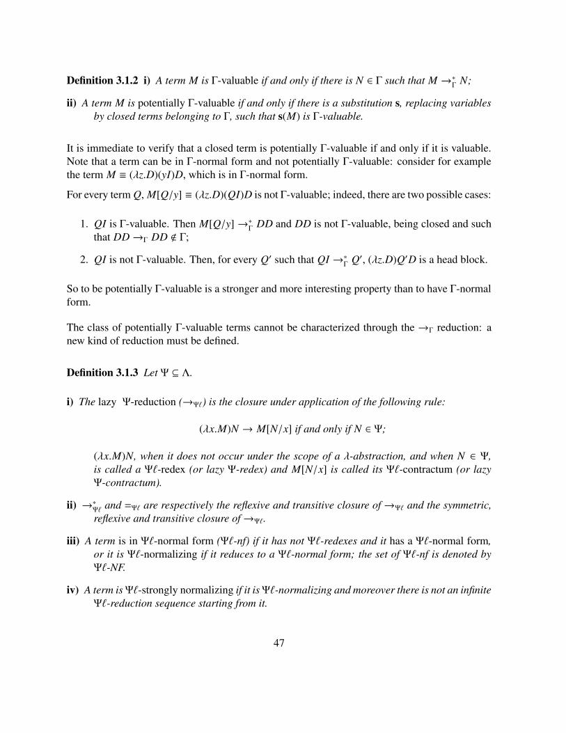
Definition 3.1.2 i) A term M is Γ-valuable if and only if there is N ∈ Γ such that M →∗Γ

N;

ii) A term M is potentially Γ-valuable if and only if there is a substitution s, replacing variablesby closed terms belonging to Γ, such that s(M) is Γ-valuable.

It is immediate to verify that a closed term is potentially Γ-valuable if and only if it is valuable.Note that a term can be in Γ-normal form and not potentially Γ-valuable: consider for examplethe term M ≡ (λz.D)(yI)D, which is in Γ-normal form.

For every term Q, M[Q/y] ≡ (λz.D)(QI)D is not Γ-valuable; indeed, there are two possible cases:

1. QI is Γ-valuable. Then M[Q/y] →∗Γ

DD and DD is not Γ-valuable, being closed and suchthat DD→Γ DD < Γ;

2. QI is not Γ-valuable. Then, for every Q′ such that QI →∗Γ

Q′, (λz.D)Q′D is a head block.

So to be potentially Γ-valuable is a stronger and more interesting property than to have Γ-normalform.

The class of potentially Γ-valuable terms cannot be characterized through the →Γ reduction: anew kind of reduction must be defined.

Definition 3.1.3 Let Ψ ⊆ Λ.

i) The lazy Ψ-reduction (→Ψ`) is the closure under application of the following rule:

(λx.M)N → M[N/x] if and only if N ∈ Ψ;

(λx.M)N, when it does not occur under the scope of a λ-abstraction, and when N ∈ Ψ,is called a Ψ`-redex (or lazy Ψ-redex) and M[N/x] is called its Ψ`-contractum (or lazyΨ-contractum).

ii) →∗Ψ` and =Ψ` are respectively the reflexive and transitive closure of→Ψ` and the symmetric,reflexive and transitive closure of→Ψ`.

iii) A term is in Ψ`-normal form (Ψ`-nf) if it has not Ψ`-redexes and it has a Ψ`-normal form,or it is Ψ`-normalizing if it reduces to a Ψ`-normal form; the set of Ψ`-nf is denoted byΨ`-NF.

iv) A term is Ψ`-strongly normalizing if it is Ψ`-normalizing and moreover there is not an infiniteΨ`-reduction sequence starting from it.

47

Let us notice that, in the previous definition, Ψ is not asked to be a set of input values. Moreover,the definition of Ψ`-reduction, at point i), is not standard. In fact, the reduction is defined byclosing the reduction rule only under application, while in the standard case the closure is underabstraction too. This allows us to formalize the notion of lazy reduction, where no reduction canbe made under the scope of a λ-abstraction.

Potentially Γ-valuable terms will be characterized by the lazy reduction induced by the followingsubset of Λ.

Definition 3.1.4 Ξ ⊆ Λ is defined as follows:

Ξ = Γ ∪ xM1. . .Mm | ∀i ≤ m Mi ∈ Ξ.

Example 3.1.5 λx.DD ∈ Ξ, xy(λx.II) ∈ Ξ, I(xy) < Ξ. Note that the last term is in Γ-normalform, while the first two are not.

We will show that terms having Ξ`-normal forms are all and only the potentially Γ-valuableterms.

Property 3.1.6 Let M ∈ Λ.A term M has Ξ`-normal form if and only if M →∗

Ξ` P, for some P ∈ Ξ.

Proof. It is easy to see that M ∈ Ξ if and only if M is a Ξ`-normal forms.

Note that Ξ is not a set of input values. In fact, it is easy too see that the contextual reduction→Ξ would not be confluent. Let P ≡ (λx.(λyz.z)(xD))D. Clearly P →Ξ P1 ≡ (λyz.z)(DD) andP→Ξ P2 ≡ (λxz.z)D, but it doesn’t exist a P3 ∈ Λ, such that P1 →∗Ξ P3 and P2 →∗Ξ P3.

Thanks to its “lazy” definition, the→Ξ` reduction enjoys all the good properties we expect.

Theorem 3.1.7 The→Ξ` reduction enjoys both the confluence and the standardization property.

Proof. See Subsection 3.1.1.

Moreover→Ξ` and→Γ reduction commutes, as proved by the following property.

Property 3.1.8Let M →Ξ` P and M →Γ Q. Then there is N such that both Q→∗

Ξ` N and P→∗Γ

N.

48

Proof. M →Ξ` P implies M is of the shape ζ ~M, where ζ is either a Γ-redex or a head block. LetM ≡ (λx.R)(z~S ) ~M. The proof is given by cases.

1. Let R→Γ R′. It is easy to see that the following diagram commutes:

(λx.R)(z~S ) ~MΓ

Ξ`

(λx.R′)(z~S ) ~M

Ξ`

R[z~S /x] ~M Γ R′[z~S /x] ~M

2. Let ~S ≡ S 1...S j...S m and let S j →Γ S ′j (1 ≤ j ≤ m). ~S ′ will denote the sequenceS 1...S ′j...S m. It is easy to see that the following diagram commutes:

(λx.R)(z~S ) ~MΓ

Ξ`

(λx.R)(z~S ′) ~M

Ξ`

R[z~S /x] ~M∗Γ R[z~S ′/x] ~M

when may be a number ≥ 0 of Γ-reductions is needed in order to deal with the copies ofz~S generated by the Ξ`-reduction.

3. Let ~M ≡ M1...M j...Mm and let M j →Γ M′j (1 ≤ j ≤ m). ~M′ will denote the sequence

M1...M′j...Mm. It is easy to see that the following diagram commutes:

(λx.R)(z~S ) ~MΓ

Ξ`

(λx.R)(z~S ) ~M′

Ξ`

R[z~S /x] ~M Γ R[z~S ′/x] ~M′

4. The cases when the Ξ` and Γ-reduction are made in disjoint subterms of either ~S or ~M areimmediate.

5. The cases when the Ξ` and Γ-reduction are made in the same subterm of either ~S or ~M canbe treated in a similar way as the previous ones.

6. Let M ≡ (λx.R)S ~M, where S ∈ Γ. Then either P ≡ Q, or one of the previous cases applies.

The→Ξ`-reduction allows a complete characterization of the potentially Γ-valuable terms.

49

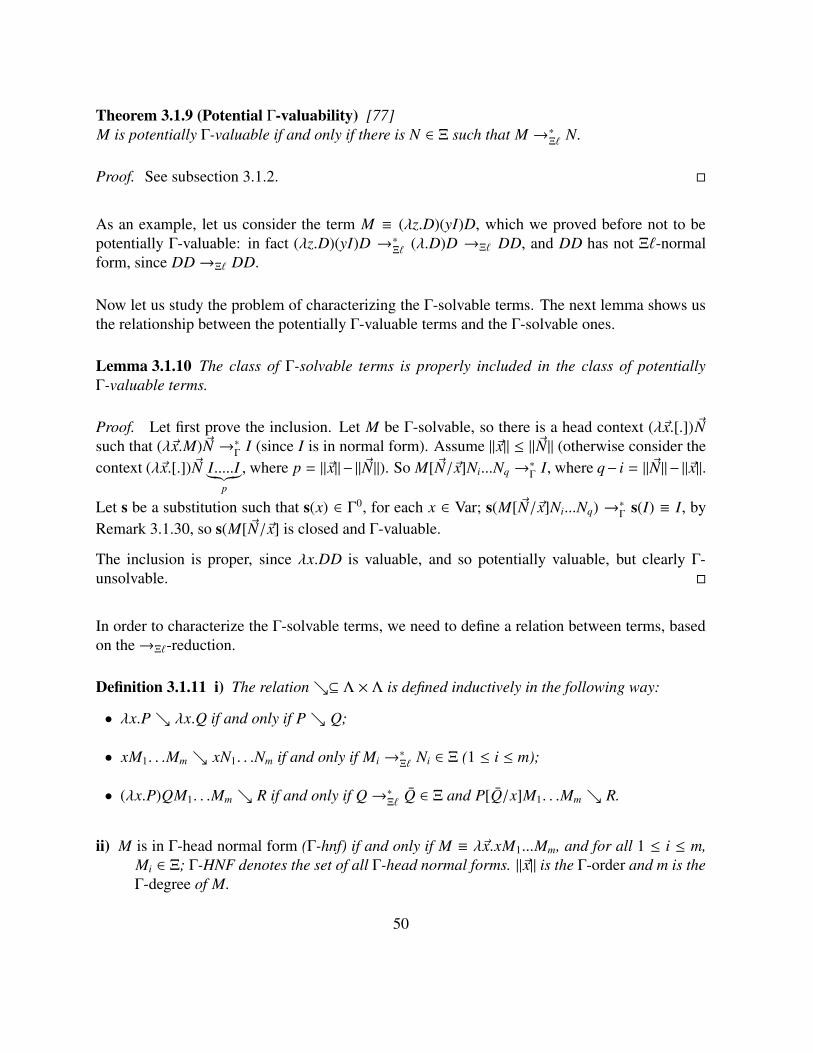
Theorem 3.1.9 (Potential Γ-valuability) [77]M is potentially Γ-valuable if and only if there is N ∈ Ξ such that M →∗

Ξ` N.

Proof. See subsection 3.1.2.

As an example, let us consider the term M ≡ (λz.D)(yI)D, which we proved before not to bepotentially Γ-valuable: in fact (λz.D)(yI)D →∗

Ξ` (λ.D)D →Ξ` DD, and DD has not Ξ`-normalform, since DD→Ξ` DD.

Now let us study the problem of characterizing the Γ-solvable terms. The next lemma shows usthe relationship between the potentially Γ-valuable terms and the Γ-solvable ones.

Lemma 3.1.10 The class of Γ-solvable terms is properly included in the class of potentiallyΓ-valuable terms.

Proof. Let first prove the inclusion. Let M be Γ-solvable, so there is a head context (λ~x.[.]) ~Nsuch that (λ~x.M)~N →∗

ΓI (since I is in normal form). Assume ‖~x‖ ≤ ‖ ~N‖ (otherwise consider the

context (λ~x.[.]) ~N I.....I︸︷︷︸p

, where p = ‖~x‖−‖~N‖). So M[~N/~x]Ni...Nq →∗Γ I, where q− i = ‖~N‖−‖~x‖.

Let s be a substitution such that s(x) ∈ Γ0, for each x ∈ Var; s(M[ ~N/~x]Ni...Nq) →∗Γ

s(I) ≡ I, byRemark 3.1.30, so s(M[ ~N/~x] is closed and Γ-valuable.

The inclusion is proper, since λx.DD is valuable, and so potentially valuable, but clearly Γ-unsolvable.

In order to characterize the Γ-solvable terms, we need to define a relation between terms, basedon the→Ξ`-reduction.

Definition 3.1.11 i) The relation⊆ Λ × Λ is defined inductively in the following way:

• λx.P λx.Q if and only if P Q;

• xM1. . .Mm xN1. . .Nm if and only if Mi →∗Ξ` Ni ∈ Ξ (1 ≤ i ≤ m);

• (λx.P)QM1. . .Mm R if and only if Q→∗Ξ` Q ∈ Ξ and P[Q/x]M1. . .Mm R.

ii) M is in Γ-head normal form (Γ-hnf) if and only if M ≡ λ~x.xM1...Mm, and for all 1 ≤ i ≤ m,Mi ∈ Ξ; Γ-HNF denotes the set of all Γ-head normal forms. ‖~x‖ is the Γ-order and m is theΓ-degree of M.

50

iii) M has Γ-head-normal form if and only if M λ~x.xM1...Mm, and Mi ∈ Ξ, for all 1 ≤ i ≤ m.

Note that Γ-HNF is a proper subclass of Λ-HNF, in fact λx.x(DD) ∈ Λ-HNF, but λx.x(DD) < Γ-HNF since DD < Ξ.

The notion of Γ-order (or simply order, when the set of input values is clear from the context)can be extended to terms not having Γ-hnf in the following way:

Definition 3.1.12 i) M is of Γ-order 0 if and only if there is no P such that M →∗Ξ` λx.P;

ii) M is of Γ-order n ≥ 1 if and only if n is the maximum integer such that M →∗Ξ` λ~x1.M1,

Mi →∗Ξ` λ ~xi + 1.Mi+1 (1 ≤ i < m) and Mm is Γ- unsolvable of order 0 and n =∑m

i=1 ‖~xi‖.If such an n does not exists M is of Γ-order∞.

Example 3.1.13 DD and (λzx.xD)(yI)D are Γ-unsolvable of order 0, xy is Γ-solvable of order0. (λxy.xx)(λxy.xx) is Γ-unsolvable of order∞.

Theorem 3.1.14 (Γ-solvability) [77]A term is Γ-solvable if and only if it has Γ-head-normal form.

Proof. See Subsection 3.1.2.

It is possible to give also an operational characterization of the Γ- solvable terms, through thenotion of Ξ`-reduction.

Property 3.1.15 M is Γ-solvable if and only if there are an integer n and terms M1, ..,Mn suchthat M →∗

Ξ` λ~x1.M1, Mi →∗Ξ` λ ~xi+1.Mi+1 (1 ≤ i < n) and Mn ≡ xP1...Pm where Pi ∈ Ξ for somem ∈ .

Proof.

(⇒) By induction on the Definition 3.1.11. If M is in Γ-hnf, then the proof is trivial. Otherwise,the only not obvious case is when M ≡ (λx.P)QM1...Mn. In this case M is Γ-solvable if andonly if Q →∗

Ξ` Q′ and P[Q′/x]M1...Mn R, and R is in Γ-hnf. By induction there are aninteger n and terms M1, ..,Mn such that P[Q′/x]M1...Mn →∗Ξ` λ~x1.M1, Mi →∗Ξ` λ ~xi+1.Mi+1

(1 ≤ i < n) and Mn ≡ xP1...Pm, for some m. Let M0 ≡ P[Q′/x]M1...Mn. Since M →∗Ξ` M0,

the proof is given.

51

(⇐) By induction on n. If n = 1, then M →∗Ξ` xM1...Mn, and so M is Γ-solvable. In all other

cases the proof follows easily by induction.

Differently from the call-by-name case, in the λΓ-calculus the notion of Γ-nf is not semanti-cally meaningful, in fact we seen that a term in Γ-nf can be not potentially valuable, and soΓ-unsolvable. Moreover, consider the two terms (λz.D)(yI)D and (λz.D)(yK)D: they are Γ-normal forms, they are ,Γ, but they are both Γ-unsolvable of Γ-order 0, and we will see that allthe Γ-unsolvable terms of Γ-order 0 can be consistently equated.

Nevertheless Λ-normal forms maintain a semantic importance also in this calculus, as the nexttheorem show. Note that a Λ-normal form is a particular case of a Ξ`-normal form.

Theorem 3.1.16 (Γ-Separability Theorem) [75] Let M,N ∈ Λ-NF.If M ,Λη N then M and N are Γ-separable.

Proof. See the subsection 3.1.3.

The Γ-Separability Theorem has an interesting semantical consequence.

Corollary 3.1.17 Let M,N be two Λ-normal forms and let M ,Λη N.For every Γ-theory T , if M =T N then T is input inconsistent.

Proof. The proof is identical to the proof of Property 1.3.6, just putting ∆ = Γ.

We proved that, for every λΛ-theory T , I =T E if and only if T is fully extensional. In case ofλΓ-calculus, we can prove only a weaker property.

Property 3.1.18 I =T E if and only if M =T λx.Mx (x < FV(M)) for every M ∈ Γ.

Proof. (⇒) I =T E implies IM =T EM, for all M. If M ∈ Γ, this in its turn implies M =T λx.Mx(x < FV(M)).(⇐) If M =T λx.Mx, for each M ∈ Γ, then x =T λy.xy, so λx.x =T λxy.xy.

The notion of fixed point can be easily extended in the call-by-value setting, in the sense that Nis a call-by-value fixed point of M if and only if MN =Γ N.

52

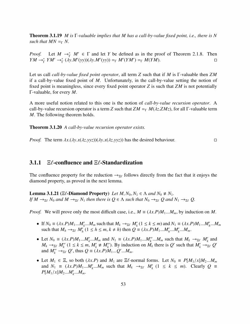
Theorem 3.1.19 M is Γ-valuable implies that M has a call-by-value fixed point, i.e., there is Nsuch that MN =Γ N.

Proof. Let M →∗Γ

M′ ∈ Γ and let Y be defined as in the proof of Theorem 2.1.8. ThenY M →∗

ΓY M′ →∗

Γ(λy.M′(yy))(λy.M′(yy)) =Γ M′(Y M′) =Γ M(Y M).

Let us call call-by-value fixed point operator, all term Z such that if M is Γ-valuable then ZMif a call-by-value fixed point of M. Unfortunately, in the call-by-value setting the notion offixed point is meaningless, since every fixed point operator Z is such that ZM is not potentiallyΓ-valuable, for every M.

A more useful notion related to this one is the notion of call-by-value recursion operator. Acall-by-value recursion operator is a term Z such that ZM =Γ M(λz.ZMz), for all Γ-valuable termM. The following theorem holds.

Theorem 3.1.20 A call-by-value recursion operator exists.

Proof. The term λx.(λy.x(λz.yyz))(λy.x(λz.yyz)) has the desired behaviour.

3.1.1 Ξ`-confluence and Ξ`-Standardization

The confluence property for the reduction →Ξ` follows directly from the fact that it enjoys thediamond property, as proved in the next lemma.

Lemma 3.1.21 (Ξ`-Diamond Property) Let M,N0,N1 ∈ Λ and N0 . N1.If M →Ξ` N0 and M →Ξ` N1 then there is Q ∈ Λ such that N0 →Ξ` Q and N1 →Ξ` Q.

Proof. We will prove only the most difficult case, i.e., M ≡ (λx.P)M1...Mm, by induction on M.

• If N0 ≡ (λx.P)M1...M′k...Mm such that Mk →Ξ` M′

k (1 ≤ k ≤ m) and N1 ≡ (λx.P)M1...M′h...Mm

such that Mh →Ξ` M′h (1 ≤ h ≤ m, k , h) then Q ≡ (λx.P)M1...M′

h...M′k...Mm.

• Let N0 ≡ (λx.P)M1...M′k...Mm and N1 ≡ (λx.P)M1...M′′

k ...Mm such that Mk →Ξ` M′k and

Mk →Ξ` M′′k (1 ≤ k ≤ m, M′

k . M′′k ). By induction on Mk there is Q′ such that M′

k →Ξ` Q′

and M′′k →Ξ` Q′, thus Q ≡ (λx.P)M1...Q′...Mm.

• Let M1 ∈ Ξ, so both (λx.P) and M1 are Ξ`-normal forms. Let N0 ≡ P[M1/x]M2...Mm

and N1 ≡ (λx.P)M1...M′k...Mm such that Mk →Ξ` M′

k (1 ≤ k ≤ m). Clearly Q ≡P[M1/x]M2...M′

k...Mm.

53

Theorem 3.1.22 (Ξ`-Confluence) Let M,N0,N1 ∈ Λ.If M →∗

Ξ` N0 and M →∗Ξ` N1 then there is P ∈ Λ such that N0 →∗Ξ` P and N1 →∗Ξ` P.

Proof. By Lemma 3.1.21, following the same reasoning as in Theorem 1.2.5.

Let M →∗Ξ` N; by the Ξ`-Confluence Theorem, M has Ξ`-normal form if and only if N has

Ξ`-normal form.

Corollary 3.1.23 The Ξ`-normal form of a term, if it exists, is unique.

In order to state a Standardization Theorem for→Ξ`, we need to redefine some notions alreadystated for λ∆-calculus. The fact that Ξ is not a set of input values forces this redefinition.

Definition 3.1.24 i) A symbol λ in a term M is Ξ`-active if and only if it is the first symbol of aΞ`-redex of M.

ii) The Ξ`-degree of a Ξ`-redex R in M is the numbers of λ’s which both are active in M andoccur on the left of R.

iii) The principal Ξ`-redex of M, if it exists, is the redex of M with minimum degree.

iv) A sequence M ≡ P0 →Ξ` P1 →Ξ` ... →Ξ` Pn →Ξ` N is standard if and only if the Ξ`-degreeof the redex contracted in Pi is less than or equal to the degree of the redex contracted inPi+1, for every i < n.

It can be easily checked that the definition of Ξ`-degree of a redex, given in the definition before,can be obtained by specializing the general notion of sequentialization given in Definition 1.2.7:its simplification is due to the lazyness of the reduction.

If M →Ξ` N by reducing a Ξ`-redex of degree k ∈ then, we will use the notation Mk→Ξ` N.

Lemma 3.1.25 Let P0k→Ξ` P1

h→Ξ` P2 and k > h.There is n ∈ and P′1 ∈ Λ such that P0

h→Ξ` P′1n→Ξ` P2 and n ≥ h.

54

Proof. By induction on P0.We will prove only the most difficult case, when P0 ≡ (λx.P)QM1...Mm (m ∈

). Note that

k > h implies k ≥ 1, so the principal redex cannot be reduced in P0k→Ξ` P1; thus either

P1 ≡ (λx.P)Q′M1...Mm where Qk→Ξ` Q′ or P1 ≡ (λx.P)QM1...M′

j...Mm where M j →Ξ` M′j

(1 ≤ j ≤ m).

• In the first case, k > h implies there is Q′′ ∈ Λ such that Q′ →Ξ` Q′′, P2 ≡ (λx.P)Q′′M1...Mm.The proof follows by induction on Q.

Note that Qk→Ξ` Q′ implies Q < Ξ; moreover, Q

k→Ξ` Q′ and k > h imply Q′ < Ξ, sincethe reduction is not principal.

• In the last case:

1. either P2 ≡ (λx.P)QM1...M′′j ...Mm where M

k′→Ξ` M′ h′→Ξ` M′′ and k′ ≥ h′;2. or P2 ≡ (λx.P)QM1...M′

j...M′r...Mm where r > j.

In case 1 the proof follows by induction on M j, in case 2 we take the reduction sequenceP0 →Ξ` (λx.P)QM1...M′

j...Mm →Ξ` P2.

Corollary 3.1.26 If P0k→Ξ` P1

0→Ξ` P2 and k ≥ 1 then there are P′1 ∈ Λ and h ∈ , such that

P00→Ξ` P′1

h→Ξ` P2.

Proof. By the Lemma 3.1.25, just putting h = 0.

Now we can state the Standardization Theorem.

Theorem 3.1.27 (Ξ`-Standardization)If M →∗

Ξ` N then there is a standard reduction sequence from M to N.

Proof. By induction on M. Let M ≡ xM1...Mm. N must be of the shape xP1...Pm, whereMi →∗Ξ` Pi. By induction there is a standard reduction sequence Mi →Ξ` Pi, and so the desiredstandard sequence is: M →

Ξ` xP1M2...Mm →Ξ` xP1P2...Mm →Ξ` xP1...Pm (1 ≤ i ≤ m).If M ≡ λx.M′ then it must be M ≡ N, and the empty reduction sequence is trivially standard.Let M ≡ (λx.P)M1...Mm (m ≥ 2). The proof follows by induction on the length of the reductionM →∗

Ξ` N, by using the previous corollary.

The principal reduction is normalizing.

55

Corollary 3.1.28 M →∗Ξ` N ∈ Ξ if and only if M

0→Ξ`

∗N ∈ Ξ.

Proof. Trivial.

3.1.2 Proof of Potential Γ-valuability and Γ-solvability Theorems

In order to prove the theorems, we need to introduce a measure for carrying out some inductiveproofs.

Definition 3.1.29 The weight 〈 〉 : Λ −→ is the partial function, defined as follows:

• 〈λx.M′〉 = 0;

• 〈xM1...Mm〉 = 1 + 〈M1〉 + ..... + 〈Mm〉;• 〈(λx.M0)M1. . .Mm〉 = 1 + 〈M1〉 + 〈M0[M1/x]M2. . .Mm〉.

In Section 3.2, we will show that the weight of a term M is defined if and only if M has Ξ`-normalform.

The following remark will be extensively used in the sequel.

Remark 3.1.30 Let M,N, P,Q ∈ ∆. If M →∆ N and P→∆ Q then M[P/z]→∆ N[Q/z].

Proof. Easy, by induction on M.

Lemma 3.1.31 Let Q ∈ Ξ, P ∈ Λ and C[.] be a context.

i) If Q ∈ Ξ then 〈Q〉 is defined.

ii) If M →Ξ` N and 〈N〉 is defined then 〈M〉 is defined.

iii) If M has Ξ`-normal form then 〈M〉 is defined.

Proof.

i) By induction on Q.

56

ii) By induction on 〈N〉.If 〈N〉 = 0 then N ≡ λx.N′, so M ≡ (λz.P)Q and Q ∈ Ξ; hence, 〈M〉 = 1 + 〈Q〉+ 〈N〉 where〈Q〉 is defined by the previous point of this lemma.Let 〈N〉 ≥ 1; there are many cases.

i) Let M ≡ xM1...Mm →Ξ` xN1...Nm ≡ N (m ≥ 1) where there is a unique k ≤ m such thatMk →Ξ` Nk while Mh ≡ Nh if h , k. The proof follows easily by induction.

ii) Let M ≡ (λz.P)QM1...Mm →Ξ` RM1...Mm ≡ N (m ≥ 1) where Q ∈ Ξ and (λz.P)Q→Ξ`

R; hence, 〈M〉 = 1 + 〈Q〉 + 〈N〉 where 〈Q〉 is defined by the previous point of thislemma.

iii) The case M ≡ λx.P is not possible, since→Ξ` is lazy.

iii) By induction on the length of the sequence to Ξ`-normal form, by using the previous pointsof this lemma.

The weight of a term allows to induce on the length of reduction sequences with respect todifferent notions of reduction.

Remark 3.1.32If M ∈ Λ0 is Γ-valuable then M is of the shape (λz.P)QM1...Mm, for some m ∈ ; moreover, Mi

is closed and Γ-valuable too (1 ≤ i ≤ m).

Property 3.1.33 Let M,N ∈ Λ0.

i) If M is Γ-valuable then 〈M〉 is defined.

ii) M →∗Λ

N and 〈M〉 is defined imply 〈N〉 is defined and 〈M〉 ≥ 〈N〉.iii) Let either M →∗

ΓN or M →∗

Ξ` N. If 〈M〉 is defined then 〈N〉 is defined and 〈M〉 ≥ 〈N〉.

Proof.

i) Γ is a standard set of input values and M →∗Γ

N ∈ Γ imply M →∗pΓ

N′ ∈ Γ; moreover, since Mis closed there is M′ such that M →p

ΓM1 →p

ΓM2... →p

ΓMr →p

Γλz.M′ →p∗

ΓN′ ∈ Γ, where

Mi is not an abstraction , for all i (1 ≤ i ≤ r). Then M →Γ` λz.M′.Clearly M →Γ` λz.M′ ∈ Γ implies M →Ξ` λz.M′ ∈ Ξ, so the proof follows by Lemma3.1.31.iii .

57

ii) Let 〈M〉 = k and let p be the numbers of steps of the standard reduction sequence M →∗Λ

N.The proof is given by induction on the pair: (k, p), ordered according to the lexicographicalorder.The cases where either 〈M〉 = 0 or p = 0 are trivial. M ≡ xM1. . .Mm is not possi-ble, since M ∈ Λ0 by hypothesis. Let M ≡ (λx.M0)M1. . .Mm, h′ = 〈M1〉 and h′′ =

〈M0[M1/x]M2. . .Mm〉, thus k = 1 + h′ + h′′.Let the reduction path be: M →Λ R1 →Λ .....→Λ Rp ≡ N (p > 0). There are three cases:

1. If R1 ≡ M0[M1/x]M2. . .Mm then 〈R1〉 = h′′ < k, so the proof follows by induction.

2. Let R1 ≡ (λx.N0)M1N2. . .Nm where ∃! j ∈ such that M j →Λ N j, while ∀i , j

Mi ≡ Ni (0 ≤ i ≤ m and i , 1).M0[M1/x]M2. . .Mm →Λ N0[M1/x]N2. . .Nm and h′′ < k imply 〈N0[M1/x]N2. . .Nm〉 ≤h′′, by induction.Thus 〈R1〉 = 1 + 〈M1〉 + 〈N0[M1/x]N2. . .Nm〉 ≤ k and the proof follows by induction.

3. Let R1 ≡ (λx.M0)N1M2. . .Mm, where M1 →Λ N1. Therefore, by induction onM0[M1/x]M2. . .Mm →∗Λ M0[N1/x]M2. . .Mm and h′′ < k, 〈M0[N1/x]M2. . .Mm〉 ≤ h′′.Again, by induction 〈M1〉 ≥ 〈N1〉. Thus the conclusion follows by definition ofweight and by induction.

iii) By the previous point of this Property, since→Ψ ⊆ →Λ, for each Ψ ⊆ Λ.

The next Lemma proves that if a term is potentially Γ-valuable, then it has Ξ`-normal form.

Lemma 3.1.34 Let M ∈ Λ, FV(M) ⊆ x1. . .xn and let s be a substitution such that s(xi) = Pi ∈Γ0. If s(M)→∗

ΓM ∈ Γ then there is N ∈ Ξ such that both M →∗

Ξ` N and s(N)→∗Γ

M.

Proof. The proof is carried out by induction on k = 〈s(M)〉, where s(M) ≡ M[P1/x1, ..., Pn/xn].

k = 0. Thus s(M) is an abstraction; there are two cases:

1. M ≡ x j and P j ≡ λz.P ∈ Λ0, so N ≡ x j.

2. M ≡ λz.P, so N ≡ λz.P.

In both cases the proof is immediate.

k > 0. s(M) ∈ Λ0, so s(M) ≡ (λu.R0)R1...Rr (r ≥ 1). Two cases are possible, according to theshape of M:

58

• M ≡ x jM1. . .Mm ( j ≤ n, 1 ≤ m). Assume P j ≡ (λz.P′), (indeed P j ∈ Γ0); thens(M) ≡ P js(M1)...s(Mm)→∗

ΓM ∈ Γ.

Since s(M) is Γ-valuable, there are Mi such that s(Mi) →∗Γ Mi ∈ Γ and 〈s(Mi)〉 <〈s(M)〉; hence, by induction there are Ni ∈ Ξ such that Mi →Ξ` Ni and s(Ni) →∗Γ Mi

(1 ≤ i ≤ m).Let N ≡ x jN1. . .Nm ∈ Ξ, thus x jM1. . .Mm →∗Ξ` x jN1. . .Nm and P js(N1)...s(Nm) →∗

Γ

P jM1. . .Mm →∗Γ M (1 ≤ i ≤ m).

• M ≡ (λz.P)QM1. . .Mm (m ≥ 0). Since s(M) is Γ-valuable, there is Q such thats(Q) →∗

ΓQ ∈ Γ and s

(P[Q/z]

)s(M1)...s(Mm) →∗

ΓM. Moreover 〈s(Q)〉 < 〈s(M)〉,

so by induction there is R ∈ Ξ such that Q →∗Ξ` R and s(R) →∗

ΓQ. However,

s(P[R/z]

)s(M1)...s(Mm)→∗

Γs(P[Q/z]

)s(M1)...s(Mm) and s

(P[Q/z]

)s(M1)...s(Mm)→∗

Γ

M imply s(P[R/z]

)s(M1)...s(Mm)→∗

ΓM and, by Property 3.1.33.iii

〈s(P[s(R)/z])s(M1)...s(Mm)〉 ≤ 〈s(P[Q/z]

)s(M1)...s(Mm)〉 < 〈s(M)〉.

Then, by induction, there is T ∈ Ξ such that P[R/z]M1. . .Mm →∗Ξ` T and s(T )→∗Γ

M.Let N ≡ T , so M ≡ (λz.P)QM1. . .Mm →∗Ξ` (λz.P)RM1. . .Mm →Ξ` P[R/z]M1. . .Mm →∗Ξ`N, so the proof is given.

The next Lemma proves that if a term has Ξ`-normal form then it is potentially Γ-valuable.

Lemma 3.1.35 Let M ∈ Λ, FV(M) ⊆ x1,. . ., xn.M →∗

Ξ` N ∈ Ξ implies that ∃h ∈ such that ∀r ≥ h, ∃Mr ∈ Γ

M[Or/x1, ...,Or/xn]→∗Γ

Mr and N[Or/x1, ...,Or/xn]→∗Γ

Mr

where Or ≡ λx1. . .xr+1.xr+1.

Proof. Let pr be the substitution such that pr(y) = Or, for all y ∈ Var and r ≥ 0; so pr(M) =

M[Or/x1, ...,Or/xn].The proof will be given by induction on 〈M〉.

• Let 〈M〉 = 0, so M is an abstraction and the proof is trivial.

• Let 〈M〉 ≥ 1. If M ≡ xM1...Mm (m ∈ ) then by induction, ∀i ≤ m there are hi ∈

suchthat ∀r ≥ maxm, h1, ..., hm, pr(Mi)→∗Γ Mr

i ∈ Γ and the proof is immediate.Otherwise, let M ≡ (λz.P)QM1. . .Mm (m ∈

); M has Ξ`-normal form implies that thereis R ∈ Ξ such that Q →∗

Ξ` R. Hence 〈Q〉 < 〈M〉 and this implies, by induction, that there

59

is h0 ∈ such that ∀r ≥ h0 ∃Qr ∈ Γ, such that pr(Q) →∗

ΓQr and pr(R) →∗

ΓQr; clearly

P[R/z]M1. . .Mm →∗Ξ` N too.By Property 3.1.33.iii 〈P[R/z]M1. . .Mm〉 ≤ 〈P[Q/z]M1. . .Mm〉 < 〈M〉 then, by induction,there is h1 ∈

such that ∀r ≥ h1 ∃Pr ∈ Γ satisfying pr(P[R/z]M1...Mm

) →∗Γ

Pr andpr(N)→∗

ΓPr.

∀r ≥ maxh0, h1, ∃Qr ∈ Λ0 pr(R)→∗Γ

Qr implies, by the Confluence Theorem,

pr(P[R/z]

)pr(M1)...pr(Mm)→∗Γ pr

(P[Qr/z]

)pr(M1)...pr(Mm)→∗Γ Pr.

Since pr(M)→∗Γ

pr(P[Qr/z]

)pr(M1)...pr(Mm), the proof is given.

Proof of Potential Γ-valuability Theorem.

The proof of the (only if) part follows directly from Lemma 3.1.34, the proof of the (if) partfollows directly from Lemma 3.1.35.

The following lemma implies as an immediate corollary that, if M ∈ Λ has Γ-head-normal formthen M is Γ-solvable.

Lemma 3.1.36 If M has Γ-head normal form and FV(M) = x1, ..., xn then ∃s ∈ , ∀r ≥ s,

∃k ∈ such that (λx1...xn.M) Or...Or︸ ︷︷ ︸

r

→∗Γ

Ok.

Proof. Let pr (r ∈ ) be the substitution such that pr(y) = Or, for each y ∈ Var.By induction on the minimum number q of steps necessary to prove that M N, for some N inΓ-head-normal form.If M is an abstraction, the proof follows directly by induction. Let M ≡ xM1...Mm, whereMi have Ξ`-normal forms (1 ≤ i ≤ m). By Lemma 3.1.35, ∃si ∈

such that ∀r ≥ si,Mi[Or/x1, ...,Or/xn] →∗

ΓMi ∈ Γ (1 ≤ i ≤ m). Let r ≥ maxm, n, s1, ..., sm, thus for some

k ∈ ,(λx1...xn.M) Or...Or

︸ ︷︷ ︸r

→∗Γ Or M1...Mm Or...Or︸ ︷︷ ︸

r−n

→∗Γ Or−m Or...Or︸ ︷︷ ︸

r−n

→∗Γ Ok.

If r − m ≥ r − n then n ≥ m and k = (r − m) − (r − n) = n − m, otherwise r − m < r − n andOr−m Or.....Or

︸ ︷︷ ︸r−n

→∗Γ

Or.....Or︸ ︷︷ ︸r−n−(r−m)

, thus r − n − (r −m) = m − n and k = r − (m − n − 1) = r + 1 + n −m.

Let M ≡ (λx.P)QM1...Mm (m ≥ 1). By definition Q →∗Ξ` R ∈ Ξ and M P[R/x]M1...Mm,

which has Γ-head-normal form. Q →∗Ξ` R ∈ Ξ implies that ∃h0 ∈ such that ∀r ≥ h0, ∃Qr ∈ Γ,

60

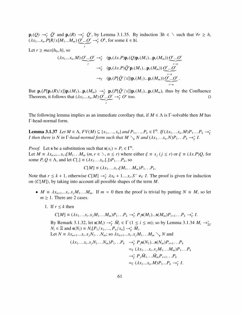
pr(Q) →∗Γ

Qr and pr(R) →∗Γ

Qr, by Lemma 3.1.35. By induction ∃h ∈ such that ∀r ≥ h,

(λx1...xn.P[R/x]M1...Mm) Or...Or︸ ︷︷ ︸

r

→∗Γ

Ok, for some k ∈ .

Let r ≥ maxh0, h, so

(λx1...xn.M) Or...Or︸ ︷︷ ︸

r

→∗Γ

(pr(λx.P)pr(Q)pr(M1)...pr(Mm)) Or...Or︸ ︷︷ ︸

r−n→∗

Γ(pr(λx.P)Qrpr(M1)...pr(Mm)) Or...Or

︸ ︷︷ ︸r−n

→Γ (pr(P[Qr/x])pr(M1)...pr(Mm)) Or...Or︸ ︷︷ ︸

r−n

.

But pr(P[pr(R)/x]

)pr(M1)...pr(Mm) →∗

Γpr

(P[Qr/x]

)pr(M1)...pr(Mm), thus by the Confluence

Theorem, it follows that (λx1...xn.M) Or...Or︸ ︷︷ ︸

r

→∗Γ

Ov too.

The following lemma implies as an immediate corollary that, if M ∈ Λ is Γ-solvable then M hasΓ-head-normal form.

Lemma 3.1.37 Let M ∈ Λ, FV(M) ⊆ x1,. . ., xn and P1,. . ., Pk ∈ Γ0. If (λx1. . .xn.M)P1. . .Pk →∗ΓI then there is N in Γ-head-normal form such that M N and (λx1. . .xn.N)P1. . .Pk →∗Γ I.

Proof. Let s be a substitution such that s(xi) = Pi ∈ Γ0.Let M ≡ λxn+1...xr.ξM1. . .Mm (m, r ∈

, n ≤ r) where either ξ ≡ x j ( j ≤ r) or ξ ≡ (λx.P)Q, forsome P,Q ∈ Λ, and let C[.] ≡ (λx1. . .xn.[.])P1. . .Pk, so

C[M] ≡ (λx1. . .xr.ξM1. . .Mm)P1. . .Pk.

Note that r ≤ k + 1, otherwise C[M] →∗Γλxk + 1....xr.S ′ ,Γ I. The proof is given for induction

on 〈C[M]〉, by taking into account all possible shapes of the term M.

• M ≡ λxn+1...xr.x jM1. . .Mm. If m = 0 then the proof is trivial by putting N ≡ M, so letm ≥ 1. There are 2 cases.

1. If r ≤ k then

C[M] ≡ (λx1. . .xr.x jM1. . .Mm)P1. . .Pk →∗Γ P js(M1)...s(Mm)Pr+1. . .Pk →∗Γ I.

By Remark 3.1.32, let s(Mi) →∗Γ Mi ∈ Γ (1 ≤ i ≤ m); so by Lemma 3.1.34 Mi →∗Ξ`Ni ∈ Ξ and s(Ni) ≡ Ni[P1/x1, ..., Pn/xn]→∗

ΓMi.

Let N ≡ λxn+1...xr.x jN1. . .Nm; so λxn+1...xr.x jM1. . .Mm N and

(λx1. . .xr.x jN1. . .Nm)P1. . .Pk →∗Γ P js(N1)...s(Nm)Pr+1. . .Pk

=Γ (λx1. . .xr.x jM1. . .Mm)P1. . .Pk

→∗Γ

P jM1. . .MmPr+1. . .Pk

=Γ (λx1...xn.M)P1...Pk →∗Γ I.

61

2. If r = k + 1 then the proof is similar to that of the previous case, since

C[M] ≡ (λx1. . .xr.x jM1. . .Mm)P1. . .Pk →∗Γ λxr.P js(M1)...s(Mm)→∗Γ λxr.xr.

• M ≡ λxn+1. . .xr.(λz.P)QM1. . .Mm (m ≥ 0, r ≥ n); there are 2 cases.

1. If r ≤ k then

C[M] ≡ (λx1. . .xr.(λz.P)QM1. . .Mm)P1. . .Pk

→∗Γ

s(λz.P)s(Q)s(M1)...s(Mm)Pr+1. . .Pk

→∗Γ

s(λz.P)Qs(M1)...s(Mm)Pr+1. . .Pk →∗Γ I

where s(Q) →∗Γ

Q ∈ Γ. Hence, by Lemma 3.1.34 Q →∗Ξ` R ∈ Ξ and s(R) →∗

ΓQ ∈ Γ;

moreovers(P[R/z]

)s(M1)...s(Mm)Pr+1. . .Pk →∗Γ

s(P[Q/z]

)s(M1)...s(Mm)Pr+1. . .Pk →∗Γ I.

Let U ≡ λxn+1. . .xr.P[R/z]M1. . .Mm, thus C[U] →∗Γ

I. Remember that P1,. . ., Pk ∈Γ0; then

〈C[M]〉 = r + 〈P1〉 + ..... + 〈Pr〉 + 〈s(λz.P)s(Q)s(M1)...s(Mm)Pr+1. . .Pk〉 =

= r + 0 + ..... + 0︸ ︷︷ ︸n

+1 + 〈s(Q)〉 + 〈s(P[s(Q)/z])s(M1)...s(Mm)Pr+1. . .Pk〉

and by Property 3.1.33.ii)

〈s(P[s(Q)/z])s(M1)...s(Mm)Pr+1. . .Pk〉 ≥ 〈s(P[s(R)/z]

)s(M1)...s(Mm)Pr+1. . .Pk〉.

Hence, 〈C[U]〉 < 〈C[M]〉 and by induction, we can state U T and C[U]→∗Γ

I, forsome T in Γ-head-normal form.Let N be T ; so C[N]→∗

ΓI and

M ≡ λxn+1. . .xr.(λz.P)QM1. . .Mm λxn+1. . .xr.P[R/z]M1. . .Mm T.

2. The case r = k + 1 is similar to the previous one.

Proof of Γ-solvability Theorem

Let FV(M) = x1,. . ., xn.

62

(⇒) By Lemma 3.1.36 for some r and h: (λx1. . .xn.M) Or.....Or︸ ︷︷ ︸

r

→∗Γ

Oh (h ≥ 0).

Let R1,. . .,Rk ∈ Γ thus (λx1. . .xn.M) Or.....Or︸ ︷︷ ︸

r

R1. . .Rk →∗Γ I.

(⇐) By Lemma 3.1.37.

3.1.3 Proof of Γ-Separability Theorem

The proof will be given in a constructive way, by showing a separability algorithm. The algo-rithm is defined as a formal system, proving statements of the shape:

M,N VΓ C[.]

where M,N are Λ-normal forms such that M ,Λη N.Differently from the call-by-name case, the context C[.] generated from the algorithm is not yetthe separating one. More precisely, it is a separating context if M,N ∈ Λ0, but for open termssome additional work must be done.

Let Bn ≡ λx1...xn+1.xn+1x1...xn, On ≡ λx1...xn+1.xn+1 and Uni ≡ λx1...xn.xi (i ≤ n, n ∈ ).

Furthermore, if S ⊆ Var then let Xnx,S ≡

λz1. . .zn. xiz1. . .zn if x < S ;

x otherwise.

The notions of args, nfΛ and 'γ are defined respectively in Definitions 2.1.13, 2.1.15 and 2.1.11.

Remark 3.1.38 It is easy to check that every Λ-normal form M is a potentially valuable term;so every subterm of a Γ-nf, being in its turn a Γ-nf, is potentially Γ-valuable.

A first problem in the development of a Separability Theorem for the Γ-calculus is the transfor-mation of potentially valuable terms (subterms) in valuable ones. As proved in the next Lemma,the solution will be to substitute to free variables some values with a suitable number of initialabstractions.

Lemma 3.1.39 Let M ∈ Λ-NF, FV(M) = x1, ..., xn and r ≥ args(M).If ∀ j ≤ n , Qr

j ≡ λx1...xr.Q j and Q j ∈ Γ then

M[Qr1/x1, ...,Qr

n/xn]→∗Γ M ∈ Γ.

63

Proof. By induction on M.

The next lemma proves an important result on which the inductive rule (Γ7) of the algorithm isbased. The relation ;γ has been defined in Definition 2.1.11.

Lemma 3.1.40 Let M,N be Λ-normal form, r ≥ maxargs(M), args(N) and y, z ∈ Var.Let Cr

k[.] ≡ (λx1...xk.[.])Xrx1,y,z...X

rxk ,y,z, for some k ∈ .

i) ∃M ∈ Λ-NF such that Crk[M]→∗

ΛM and r ≥ args(M).

ii) If M ;γ N then nfΛ(Crk[M]) ;γ nfΛ(Cr

k[N]).

Proof.

i) By induction on M.If M ≡ λu.P or M ≡ uM1...Mm (where u < x1, ..., xk and m ≤ r) then the proof follows byinduction. Let M ≡ x jM1...Mm (1 ≤ j ≤ k, m ≤ r); so by induction ∀i ≤ m there is Mi ∈ Λ-NF such that Cr

k[Mi] →∗Λ Mi and r ≥ args(Mi). If x j ∈ y, z the proof is immediate, sinceXr

x j,y,z ≡ x j. Let x j < y, z; clearly

Crk[M] ≡ (λx1...xk.x jM1...Mm)Xr

x1,y,z...Xrxk ,y,z →∗Λ

(λu1. . .ur.x ju1. . .ur)M1...Mm →∗Λ λum+1. . .ur.x jM1...Mmum+1. . .ur;

so r ≥ maxr, args(M1), ..., args(Mm), 0, ....., 0︸ ︷︷ ︸r−m

= r. Note that nfΛ(Crk[M]) is well defined.

ii) Let M ≡ λu1. . .up.uM1. . .Mm and N ≡ λv1. . .vq.vN1. . .Nn; we reason by induction on γ. Letγ ≡ ε, |p − m| , |q − n| and v ≡ u.∀i Mi ≡ nfΛ(Cr

k[Mi]) and Ni ≡ nfΛ(Crk[Ni]). Let u ≡ v ≡ x j, for some j ≤ k and u, v < y, z,

otherwise the proof is simpler, thus

nfΛ(Crk[M]) ≡ λu1. . .upwm+1. . .wr.x jM1...Mmwm+1. . .wr

nfΛ(Crk[N]) ≡ λv1. . .vqwn+1. . .wr.x jN1...Nnwn+1. . .wr

|(p + (r − m)) − (m + (r − m))| , |(q + (r − n)) − (n + (r − n))|, since |p − m| , |q − n|.If x . y the proof is similar.If γ ≡ i, γ′ (where i ≥ 1) then the proof follows by induction.

64

The Algorithm is presented in figure 3.1 (pag. 66). For sake of simplicity, in the algorithmdescription, we assume that different bound variables have different names.The algorithm follows essentially the same pattern than the call-by-name separability algorithm,but the context in the conclusion replaces variables by terms having enough initial abstractionsto assure that subterms become Γ-valuable, by using the result of Lemma 3.1.39.Note that, in rules (Γ3)-(Γ6), every occurrence of the term Br in the context could be safelyreplaced by I, so following an approach more similar to the call-by-name case. In fact suchterms will be erased when the context, filled by one of the two input terms, will be Γ-reduced.Using Br allows an easier correctness proof.

Example 3.1.41 Let M ≡ λxyu.x(u(x(yy))(vv)) and N ≡ λxyu.x(u(yy)(vv)), i.e. the same termsof Example 2.1.17.

Clearly args(M) = args(N) = 2, so let r = 2. The derivation proving the statement M,N VΓ C[.]is the following:

x3 . y C5[.] ≡ (λx3y.[.])(λx1x2x3x4.x)(λx1x2x3x4x5.y)II(Γ5)

x3(yy)(λv1v2.x2v1v2) ,,, yy(λv1v2.x2v1v2)x3 VΓ C5[.](Γ2)

λx2x3.x3(yy)x2 ,,, yyVΓ C2[.] ≡ C5[[.](λv1v2.x2v1v2)x3](Γ6)

u(λx2x3.x3(yy)x2)(vv) ,,, u(yy)(vv)VΓ C6[.] ≡ C2[(λu.[.])(λz1z2.z1)](Γ7)

x(u(x(yy))(vv)) ,,, x(u(yy)(vv))VΓ C7[.] ≡ C6[(λx.[.])(λx1x2x3.x3x1x2)I(λz1z2.z1)](Γ1)

λxyu.x(u(x(yy))(vv)) ,,, λxyu.x(u(yy)(vv))VΓ C7[[.]xy(λu1u2.uu1u2)]

where, if X4 ≡ (λx1x2x3x4.x) and Y5 ≡ (λx1x2x3x4x5.y):

C5[.] ≡ (λx3y. [.]

)X4Y5II

C2[.] ≡ (λx3y. [.] (λv1v2.x2v1v2)x3

)X4Y5II

C6[.] ≡ (λx3y.

((((λu. [.] )))U1

2(λv1v2.x2v1v2)x3))

X4Y5IIC7[.] ≡ (

λx3y.((((λu.(λx. [.] )B2IU1

2)))U12(λv1v2.x2v1v2)x3

))X4Y5II

C[.] ≡ (λx3y.

((((λu.(λx. [.] xy(λu1u2.uu1u2))B2IU1

2)))U12(λv1v2.x2v1v2)x3

))X4Y5II

We can check that(C[M]

)[O2/v]→∗

Γx, in fact

65

Let M,N ∈ Λ-NF, M ;γ N, r ≥ maxargs(M), args(N) and x, y be fresh variables suchthat x . y.

The rules of the system proving statements M,N VΓ C[.], are the followings:

p ≤ q Crk[.] ≡ (λx1...xk.[.])Xr

x1,x,y...Xrxk ,x,y (((k∈p,q)))

xnfΛ(Crp[M1])...nfΛ(Cr

p[Mm])Xrxp+1,x,y...X

rxq,x,y,

ynfΛ(Crq[N1])...nfΛ(Cr

q[Nn])

VΓ C[.]

(Γ1)λx1. . .xp.xM1. . .Mm, λx1. . .xq.yN1. . .Nn VΓ C[[.]Xr

x1,x,y...Xrxq,x,y]

p > q Crk[.] ≡ (λx1...xk.[.])Xr

x1,x,y...Xrxk ,x,y (((k∈p,q)))

xnfΛ(Crp[M1])...nfΛ(Cr

p[Mm]),

ynfΛ(Crq[N1])...nfΛ(Cr

q[Nn])Xrxq+1,x,y...X

rxp,x,y

VΓ C[.]

(Γ2)λx1. . .xp.xM1. . .Mm, λx1. . .xq.yN1. . .Nn VΓ C[[.]Xr

x1,x,y...Xrxp,x,y]

n < m(Γ3)

xM1. . .Mm, xN1. . .Nn VΓ (λx.[.])Or+n Br.....Br︸ ︷︷ ︸

r+n−m

(λx1. . .xm−n.x) y.....y︸︷︷︸m−n

m < n(Γ4)

xM1. . .Mm, xN1. . .Nn VΓ (λx.[.])Or+m Br.....Br︸ ︷︷ ︸

r+m−n

(λx1. . .xn−m.y) x.....x︸︷︷︸n−m

x . y(Γ5)

xM1. . .Mm, yN1. . .Nn VΓ (λxy.[.])(λx1. . .xr+m.x)(λx1. . .xr+n.y) Br.....Br︸ ︷︷ ︸

r

Mk ,Λη Nk x < FV(Mk) ∪ FV(Nk) Mk,Nk VΓ C[.](Γ6)

xM1. . .Mm, xN1. . .Nm VΓ C[(λx.[.])Urk Br.....Br︸ ︷︷ ︸

r−m

]

Mk ,Λη Nk x ∈ FV(Mk) ∪ FV(Nk)

Crx[.] ≡ (λx.[.])Br nfΛ(Cr

x[Mk]), nfΛ(Crx[Nk])VΓ C[.]

(Γ7)xM1. . .Mm, xN1. . .Nm VΓ C[Cr

x[.] Br.....Br︸ ︷︷ ︸

r−m

Urk]

Figure 3.1: Call By Value Separability Algorithm.66

(λx3y.

((((λu.(λx.M[O2/v]xy(λu1u2.uu1u2))B2IU1

2)))U12(λv1v2.x2v1v2)x3

))X4Y5II →∗

Γ(λx3y.

((((λu.M[O2/v]B2y(λu1u2.uu1u2)IU1

2)))U12(λv1v2.x2v1v2)x3

))X4Y5II →∗

Γ(λx3y.

(M[O2/v]B2y(λu1u2.U1

2u1u2)IU12(λv1v2.x2v1v2)x3

))X4Y5II →∗

Γ

(((λxyu.x(u(x(yy))(vv)))))[O2/v]B2Y5(λu1u2.U12u1u2)IU1

2(λv1v2.x2v1v2)X4II →∗Γ

(((λxyu.x(u(x(yy))(O2O2))))B2Y5(λu1u2.u1)IU12(λv1v2.x2v1v2)X4II →∗

Γ

B2((λu1u2.u1)(B2(Y5Y5))(O2O2))IU1

2(λv1v2.x2v1v2)X4II →∗Γ

B2((λu1u2.u1)(B2(λx2x3x4x5.y))O1)IU12(λv1v2.x2v1v2)X4II →∗

Γ

B2((λu1u2.u1)(λx2x3.x3(λx2x3x4x5.y)x2)O1)IU12(λv1v2.x2v1v2)X4II →∗

Γ

B2(λx2x3.x3(λx2x3x4x5.y)x2)IU1

2(λv1v2.x2v1v2)X4II →∗Γ

U12(λx2x3.x3(λx2x3x4x5.y)x2

)I(λv1v2.x2v1v2)X4II →∗

Γ(λx2x3.x3(λx2x3x4x5.y)x2

)(λv1v2.x2v1v2)X4II →∗

Γ

X4(λx2x3x4x5.y)(λv1v2.x2v1v2)II →∗Γ

x

while(C[N]

)[O2/v]→∗

Γy; in fact

(λx3y.

((((λu.(λx.N[O2/v]xy(λu1u2.uu1u2))B2IU1

2)))U12(λv1v2.x2v1v2)x3

))X4Y5II →∗

Γ(λx3y.

((((λu.(N[O2/v]B2y(λu1u2.uu1u2)IU1

2)))U12(λv1v2.x2v1v2)x3

))X4Y5II →∗

Γ(λx3y.N[O2/v]B2y(λu1u2.U1

2u1u2)IU12(λv1v2.x2v1v2)x3

)X4Y5II →∗

Γ

(((λxyu.x(u(yy)(O2O2)))))B2Y5(λu1u2.U12u1u2)IU1

2(λv1v2.x2v1v2)X4II →∗Γ

B2((λu1u2.U12u1u2)(Y5Y5)(O2O2)

)IU1

2(λv1v2.x2v1v2)X4II →∗Γ

B2((λu1u2.u1)(λx2x3x4x5.y)O1)IU12(λv1v2.x2v1v2)X4II →∗

Γ

B2(λx2x3x4x5.y)IU12(λv1v2.x2v1v2)X4II →∗

Γ

U12(λx2x3x4x5.y)I(λv1v2.x2v1v2)X4II →∗

Γ

(λx2x3x4x5.y)(λv1v2.x2v1v2)X4II →∗Γ

y

Lemma 3.1.42 (Termination) If M,N ∈ Λ-NF and M ;γ N then M,N VΓ C[.].

Proof. By induction on γ. Similar to the termination proof of the Bohm Theorem, by usingLemma 3.1.40.

The next Lemma is necessary for proving the correctness.

Lemma 3.1.43 Let zP1...Pm,T ∈ Λ-NF, args(zP1...Pm) ≤ r, args(T ) ≤ r.Let D[.] ≡ (λu1...uk.[.])R1...Rh be a context (k ≤ h) such that either R j ≡ λx1...xr.R j (1 ≤ j ≤ h)and nfΛ(D[T ]) ≡ zP1...Pm.

67

Let b denote a substitution such that, if y ∈ FV(D[T ]) then there is Qy ∈ Λ and b(y) = λx1...xr.Qy.If x1, ..., xr < FV(Qz) then b(((D[T ])))→∗

Γλxr−m...xr.Qz.

Proof. By induction on h.

h = 0 Clearly D[.] ≡ [.], so T must be zP1...Pm. b(((P j)))→∗Γ P j ∈ Γ (1 ≤ j ≤ m), by Lemma 3.1.39;so, b(((zP1...Pm))) ≡ (λx1...xr.Qz)b(((P1)))...b(((Pm)))→∗

Γ(λx1...xr.Qz)P1...Pm →∗Γ λxr−m...xr.Qz.

h ≥ 1 If k = 0 then TR1...Rh →∗Γ zP1...Pm, so the proof is similar to the previous case.Let k ≥ 1, let D′[.] be [.]Rk+1...Rh and b′ denote a substitution such that b′(u j) = R j

(1 ≤ j ≤ k) while b′(y) = b(y) for all other variables. Hence, b′(((D′[T ]))) →∗Γλxr−m...xr.Qz

by case k = 0; the proof follows, since b(((D[zP1...Pm])))→∗Γ

b′(((D′[T ]))).

Lemma 3.1.44 (Correctness)Let M,N be different Λ-normal forms such that r ≥ maxargs(M), args(N).If M,N VΓ C[.] and

(FV(C[M]) ∪ FV(C[N])

)= u1, ..., un − x, y then

(λu1...un.C[M]) Or...Or︸ ︷︷ ︸

n

→∗Γ

x and (λu1...un.C[N]) Or...Or︸ ︷︷ ︸

n

→∗Γ

y.

Proof. Let e be a substitution such that e(x) = x, e(y) = y, while ∀z ∈ Var − x, y, e(z) = Or.We will prove that e(C[M])→∗

Γx and e(C[N])→∗

Γy;

moreover, let T ∈ Λ-NF, let args(T ) ≤ r, let D[.] ≡ (λu1...uk.[.])R1...Rh be a context (k ≤ h) suchthat either R j = Br or R j = Ur

t or R j = Xru,S (where 1 ≤ j ≤ h, t ≤ r, u ∈ Var and S ⊆ Var) and let

x, y < FV(D[T ]), we will prove yet:

• if nfΛ(D[T ]) ≡ M then e(((C[D[T ]])))→∗Γ

x;

• if nfΛ(D[T ]) ≡ N then e(((C[D[T ]])))→∗Γ

y.

The proof is given by induction on the derivation proving M,N VΓ C[.].

(Γ1) Let Crp[.] ≡ (λx1...xp.[.])Xr

x1,x,y...Xrxp,x,y. The hypothesis is

xnfΛ(Crp[M1])...nfΛ(Cr

p[Mm])Xrxp+1,x,y...X

rxq,x,y,

ynfΛ(Crq[N1])...nfΛ(Cr

q[Nn])

VΓ C[.]

68

By induction,

e(((C[xnfΛ(Crp[M1])...nfΛ(Cr

p[Mm])Xrxp+1,x,y...X

rxq,x,y])))→∗Γ x

moreover, if T ∈ Λ-NF, args(T ) ≤ r, D[.] ≡ (λu1...uk.[.])R1...Rh is a context (k ≤ h)where R j ∈ Br,Ur

t , Xru,S | t ∈ ∧ u ∈ Var ∧ S ⊆ Var (1 ≤ j ≤ h), nfΛ(D[T ]) ≡

xnfΛ(Crp[M1])...nfΛ(Cr

p[Mm])Xrxp+1,x,y...X

rxq,x,y and x, y < FV(D[T ]) then e(((C[D[T ]])))→∗

Γx.

Let T ≡ xM1. . .Mm and D[.] ≡ Crp[.]; so, args(T ) ≤ r, x, y < FV(D[T ]) and nfΛ(Cr

p[T ]) ≡xnfΛ(Cr

p[M1])...nfΛ(Crp[Mm])Xr

xp+1,x,y...Xrxq,x,y imply, by induction, e

(C[D[xM1. . .Mm]]

)→∗

Γ

x, soe(C[(λx1. . .xp.xM1. . .Mm)Xr

x1,x,y...Xrxq,x,y]

)→∗Γ x.

We must yet prove that, if T ∗ ∈ Λ-NF, D∗[.] ≡ (λu∗1...u∗k∗ .[.])R

∗1...R

∗h∗ is a context (k∗ ≤ h∗)

such that either R∗j = Br or R∗j = Urt or R∗j = Xr

u,S (where 1 ≤ j ≤ h∗, t ∈ , u ∈ Var and

S ⊆ Var), args(T ∗) ≤ r, x, y < FV(D∗[M∗]) and nfΛ(D∗[T ∗]) ≡ λx1. . .xp.xM1. . .Mm thene(((C∗[D∗[T ∗]])))→∗

Γx, where C∗[.] ≡ C[[.]Xr

x1,x,y...Xrxq,x,y].

Let T ≡ T ∗ and D[.] ≡ D∗[.]Xrx1,x,y...X

rxq,x,y; thus, both

nfΛ(D∗[M∗]Xrx1,x,y...X

rxq,x,y) ≡ xnfΛ(Cr

p[M1])...nfΛ(Crp[Mm])Xr

xp+1,x,y...Xrxq,x,y,

args(T ) ≤ r and x, y < FV(D[T ∗]) imply, by induction,

e(C[D[T ∗]]

)≡ e

(C∗[D∗[T ∗]]

)→∗Γ x.

The proof for the term on the right is similar.

(Γ2) Similar to (Γ1).

(Γ3) Let n < m and let xM1. . .Mm, xN1. . .Nn VΓ C[.] where

C[.] ≡ (λx.[.])Or+n Br.....Br︸ ︷︷ ︸

r+n−m

(λx1. . .xm−n.x) y.....y︸︷︷︸m−n

.

We will prove that, if T ∈ Λ-NF, args(T ) ≤ r, D[.] ≡ (λu1...uk.[.])U1...Uh is a con-text (h, k ∈

) where R j ∈ Br,Urt , X

ru,S | t ∈ ∧ u ∈ Var ∧ S ⊆ Var (1 ≤ j ≤ h),

x, y < FV(D[T ]) and nfΛ(D[T ]) ≡ xM1. . .Mm then e(((C[D[T ]])))→∗Γ

x.Let b(x) = Or+n and b(y) = e(y) for all other variables; thus, by Lemma 3.1.43, b(((D[T ]))))→∗

Γ

Or+n−m, hence

e((λx.D[T ])Or+n Br.....Br

︸ ︷︷ ︸r+n−m

(λx1. . .xm−n.x) y.....y︸︷︷︸m−n

)→∗Γ Or+n−m Br.....Br

︸ ︷︷ ︸r+n−m

(λx1. . .xm−n.x) y.....y︸︷︷︸m−n

→∗Γ x

69

On the other hand, we will prove that, if T ∈ Λ-NF, args(T ) ≤ r, D[.] ≡ (λu1...uk.[.])U1...Uh

is a context (h, k ∈ ) where R j ∈ Br,Ur

t , Xru,S | t ∈

∧ u ∈ Var ∧ S ⊆ Var (1 ≤ j ≤ h),x, y < FV(D[T ]) and nfΛ(D[T ]) ≡ xN1. . .Nn then e(((C[D[T ]])))→∗

Γy.

Let b(x) = Or+n and b(y) = e(y) for all other variables; thus, by Lemma 3.1.43, b(((D[T ]))))→∗Γ

Or, hence

e((λx.D[T ])Or+n Br.....Br

︸ ︷︷ ︸r+n−m

(λx1. . .xm−n.x) y.....y︸︷︷︸m−n

)→∗Γ Or Br.....Br (λx1. . .xm−n.x) y.....y︸ ︷︷ ︸

r+1

→∗Γ y.

(Γ4) Symmetric to (Γ3).

(Γ5) Let xM1. . .Mm, yN1. . .Nn VΓ C[.] where C[.] ≡ (λxy.[.])(λx1. . .xr+m.x)(λx1. . .xr+n.y) Br.....Br︸ ︷︷ ︸

r

.

We will prove that, if T ∈ Λ-NF, args(T ) ≤ r, D[.] ≡ (λu1...uk.[.])U1...Uh is a con-text (h, k ∈

) where R j ∈ Br,Urt , X

ru,S | t ∈ ∧ u ∈ Var ∧ S ⊆ Var (1 ≤ j ≤ h),

x, y < FV(D[T ]) and nfΛ(D[T ]) ≡ xM1. . .Mm then e(((C[D[T ]])))→∗Γ

x.Let b(x) = λx1. . .xr+m.x, b(y) = λx1. . .xr+n.y and b(z) = e(z) for each other variable z; thus,by Lemma 3.1.43, b(((D[T ]))))→∗

Γλx1. . .xr.x, hence

e((λxy.xM1. . .Mm)(λx1. . .xr+m.x)(λx1. . .xr+n.y) Br.....Br

︸ ︷︷ ︸r

)→∗

Γx.

On the other hand, we will prove that, if T ∈ Λ-NF, args(T ) ≤ r, D[.] ≡ (λu1...uk.[.])U1...Uh

is a context (h, k ∈ ) where R j ∈ Br,Ur

t , Xru,S | t ∈

∧ u ∈ Var ∧ S ⊆ Var (1 ≤ j ≤ h),x, y < FV(D[T ]) and nfΛ(D[T ]) ≡ yN1. . .Nn then e(((C[D[T ]])))→∗

Γy.

Let b(x) = λx1. . .xr+m.x, b(y) = λx1. . .xr+n.y and b(z) = e(z) for each other variable z; thus,by Lemma 3.1.43, b(((D[T ]))))→∗

Γλx1. . .xr.y, hence

e((λxy.yN1. . .Nn)(λx1. . .xr+m.x)(λx1. . .xr+n.y) Br.....Br

︸ ︷︷ ︸r

)→∗

Γy.

(Γ6) Let Mk ,Λη Nk, x < FV(Mk) ∪ FV(Nk) and Mk,Nk VΓ C[.].By induction e(((C[Mk])))→∗Γ x; moreover, if T ∈ Λ-NF, args(T ) ≤ r, D[.] ≡ (λu1...uk.[.])R1...Rh

is a context (k ≤ h) where R j ∈ Br,Urt , X

ru,S | t ∈ ∧ u ∈ Var ∧ S ⊆ Var (1 ≤ j ≤ h),

nfΛ(D[T ]) ≡ Mk and x, y < FV(D[T ]) then e(((C[D[T ]])))→∗Γ

x.

Let T ≡ xM1. . .Mm and D[.] ≡ (λx.[.])Urk Br.....Br︸ ︷︷ ︸

r−m

; so , args(T ) ≤ r, x, y < FV(D[T ]) and

nfΛ(D[T ]) ≡ Mk imply, by induction,

e(C[D[T ]]

)≡ e

(C[(λx.xM1. . .Mm)Ur

k Br.....Br︸ ︷︷ ︸

r−m

])→∗Γ x.

We must yet prove that, if T ∗ ∈ Λ-NF, D∗[.] ≡ (λu∗1...u∗k∗ .[.])R

∗1...R

∗h∗ is a context (k∗ ≤ h∗)

such that either R∗j = Br or R∗j = Urt or R∗j = Xr

u,S (where 1 ≤ j ≤ h∗, t ∈ , u ∈ Var and

S ⊆ Var), args(T ∗) ≤ r, x, y < FV(D∗[M∗]) and nfΛ(D∗[T ∗]) ≡ xM1. . .Mm then

70

e(((C∗[D∗[T ∗]])))→∗Γ

x, where C∗[.] ≡ C[(λx.[.])Urk Br.....Br︸ ︷︷ ︸

r−m

].

Let D[.] ≡ (λxu∗1...u∗k∗ .[.])U

rkR∗1[Ur

k/x]...R∗h∗[Urk/x] Br.....Br

︸ ︷︷ ︸r−m

and T ≡ T ∗; thus, both R∗j[Urk/x] ∈

Br,Urt , X

ru,S | t ∈

∧u ∈ Var∧S ⊆ Var (1 ≤ j ≤ h∗), nfΛ(D[T ]) ≡ Mk (since x < FV(Mk)),args(T ) ≤ r and x, y < FV(D[T ]) implying, by induction,

e(C[(λx.D∗[T ∗])Ur

k Br.....Br︸ ︷︷ ︸

r−m

])

=Γ e(C[D[T ]]

)→∗Γ x.

The proof for the term on the right is similar.

(Γ7) Let Mk ,Λη Nk, x ∈ FV(Mk) ∪ FV(Nk), Crx[.] ≡ (λx.[.])Br and nfΛ(Cr

x[Mk]), nfΛ(Crx[Nk])VΓ

C[.].By induction e(((C[nfΛ(Cr

x[Mk])]))) →∗Γ x; moreover, if T ∈ Λ-NF, args(T ) ≤ r, D[.] ≡(λu1...uk.[.])R1...Rh is a context (k ≤ h) where R j ∈ Br,Ur

t , Xru,S | t ∈

∧u ∈ Var∧S ⊆ Var(1 ≤ j ≤ h), nfΛ(D[T ]) ≡ nfΛ(Cr

x[Mk]) and x, y < FV(D[T ]) then e(((C[D[T ]])))→∗Γ

x.

Let T ≡ xM1. . .Mm and D[.] ≡ (λx.[.])Br Br.....Br︸ ︷︷ ︸

r−m

Urk; so , args(T ) ≤ r, x, y < FV(D[T ])

and nfΛ(D[T ]) ≡ nfΛ(Crx[Mk]) imply, by induction,

e(C[D[T ]]

)≡ e

(C[(λx.xM1. . .Mm)Br Br.....Br

︸ ︷︷ ︸r−m

Urk])→∗Γ x.

We must yet prove that, if T ∗ ∈ Λ-NF, D∗[.] ≡ (λu∗1...u∗k∗ .[.])R

∗1...R

∗h∗ is a context (k∗ ≤ h∗)

such that either R∗j = Br or R∗j = Urt or R∗j = Xr

u,S (where 1 ≤ j ≤ h∗, t ∈ , u ∈ Var and

S ⊆ Var), args(T ∗) ≤ r, x, y < FV(D∗[M∗]) and nfΛ(D∗[T ∗]) ≡ xM1. . .Mm thene(((C∗[D∗[T ∗]])))→∗

Γx, where C∗[.] ≡ C[(λx.[.])Br Br.....Br

︸ ︷︷ ︸r−m

Urk].

Let D[.] ≡ (λxu∗1...u∗k∗ .[.])B

rR∗1[Br/x]...R∗h∗[Br/x] Br.....Br

︸ ︷︷ ︸r−m

Urk and T ≡ T ∗; thus, both R∗j[B

r/x] ∈Br,Ur

t , Xru,S | t ∈ ∧ u ∈ Var ∧ S ⊆ Var (1 ≤ j ≤ h∗), nfΛ(D[T ]) ≡ nfΛ(Cr

x[Mk]),args(T ) ≤ r and x, y < FV(D[T ]) implying, by induction,

e(C[(λx.D∗[T ∗])Br Br.....Br

︸ ︷︷ ︸r−m

Urk])

=Γ e(C[D[T ]]

)→∗Γ x.

The proof for the term on the right is similar.

Proof of Call By Value Separability Theorem

The proof follows directly from Lemmas 3.1.42 and 3.1.44.

71

3.2 Potential Valuability and Λ-reduction

In this section the relation between the call-by-value λΓ-calculus and the call-by-name λΛ-calculus will be explored. In particular we will show that the Γ-potentially valuable terms, whichhave been characterized through the notion of Ξ`-reduction, introduced on purpose, coincide withthe strongly normalizing terms with respect to the Λ`-reduction. The notion of Λ`-reduction isa particular case of Definition 3.1.3. In order to prove the result the notion of weight of a term,introduced in Definition 3.1.29, will be used.

Lemma 3.2.1 If 〈M〉 is defined then M has Ξ`-normal form.

Proof. By induction on 〈M〉.

〈M〉 = 0 Trivial, since M is an abstraction.

〈M〉 ≥ 1 If M ≡ xM1...Mm (m ∈ ) the proof follows by induction. Let M ≡ (λx.P)QM1...Mm

(m ∈ ). By induction P[Q/x]M1...Mm and Q have Ξ`-normal forms, so let Q→∗Ξ` R ∈ Ξ;

by Property 3.1.33.ii

〈P[R/x]M1...Mm〉 ≤ 〈P[Q/x]M1...Mm〉 < 〈M〉so the proof follows by induction.

Corollary 3.2.2 M has Ξ`-normal form if and only if 〈M〉 is defined.

Proof. By the previous Lemma and Lemma 3.1.31.iii.

The next lemma proves that the notion of weight works well also for the Λ`-reduction.

Lemma 3.2.3 Let M ∈ Λ and 〈M〉 be defined. If M →Λ` N then 〈N〉 is defined and 〈N〉 < 〈M〉.

Proof. The proof is given by induction on k = 〈M〉.The cases where k = 0 is not possible, since M cannot be an abstraction; so let k ≥ 1. IfM ≡ xM1. . .Mm then the proof follows by induction. Let M ≡ (λx.M0)M1. . .Mm, h′ = 〈M1〉 andh′′ = 〈M0[M1/x]M2. . .Mm〉, thus k = 1 + h′ + h′′. There are only three cases, by the lazyness of→Λ`.

72

1. If N ≡ M0[M1/x]M2. . .Mm then the proof follows from the definition of weigh.

2. Let N ≡ (λx.M0)M1N2. . .Nm where there is a unique j ≥ 2 such that M j →Λ N j, while∀i , j Mi ≡ Ni (0 ≤ i ≤ m and i , 1).M0[M1/x]M2. . .Mm →Λ` M0[M1/x]N2. . .Nm and h′′ < k imply 〈N0[M1/x]N2. . .Nm〉 < h′′,by induction. Thus 〈N〉 = 1 + 〈M1〉 + 〈N0[M1/x]N2. . .Nm〉 < k.

3. Let N ≡ (λx.M0)N1M2. . .Mm, where M1 →Λ` N1. By Property 3.1.33.ii we can state〈M0[N1/x]M2. . .Mm〉 ≤ h′′, since M0[M1/x]M2. . .Mm →∗Λ M0[N1/x]M2. . .Mm. Again, byinduction 〈M1〉 < 〈N1〉; so, the proof follows by definition of weight.

Theorem 3.2.4 M has Ξ`-normal form if and only if M is Λ`-strongly normalizing.

Proof. (⇐) Trivial, since→Ξ`⊆→Λ`.(⇒) By Corollary 3.2.2 and Lemma 3.2.3.

The follows corollary shows the desired result.

Corollary 3.2.5 Let M ∈ Λ0.M is Γ-valuable if and only if M is Λ`-strongly normalizing.

Proof. From Theorems 3.1.14 and 3.2.4.

73

Part II

Parametric Semantics

74

II. Introduction

In the literature about λ-calculus, two notions of standardization have been defined, the classicalone [6], and a strong one [57]. According to the former, a given reduction sequence can bestandardized in more than one way, while, according to the latter, there is just one standardreduction sequence corresponding to a given one. The second approach has been chosen for λ∆-calculi. Thus the standardization implies the existence of a principal reduction strategy (reducingalways the first redex in the “sequentialization”), which is normalizing. We show as variousoperational semantics can be defined in a uniform, parametric way following the normalizingstrategy. Namely we define a reduction machine, parametric with respect to both a set of inputvalues ∆ and a set of output values Θ, that implements such a strategy, and that can be seen as a”universal λ-machine”. The notion of output values seems to capture in a formal way the notionof “stable relevant minimal information” considered in [5, 30].

The machine is described in a logical form. Standard reduction machines, as that one performingthe evaluation to head normal form for the λ-calculus or a pure (without constants) version ofS.E.C.D. machine of Landin [59] can be obtained from it just instantiating ∆ and Θ in suitableways. We will show that any well-done instance of ∆ and Θ the induced contextual equivalenceis a theory, correct with respect to the considered calculus.

We have considered the sets of input valuable terms ∆? = M ∈ Λ | M →∆ P ∈ ∆ and of outputvaluable terms Θ? = M ∈ Λ | M →∆ P ∈ Θ. They produce different evaluations but, under fewconditions, inducing the same operational equivalence of the starting sets.

We study three instances of call-by-name operational semantics and a call-by-value one: theevaluation to Λ-head normal forms [53, 102], to Λ-lazy head normal forms [2, 81, 7, 71], theevaluation to Λ-normal form [53, 102] and the evaluation to Γ-lazy blocked normal form [81].In particular, we give a common notion of relevant contexts, as a generalization of the notionintroduced by Plotkin in [84]:

a context C[.] is relevant whenever there exist two terms M,N on which the contexthas different operational behaviour, namely C[M] can reduced to an output value,while C[N] not.

We given some characterization in all the four semantics considered and we used they in orderto show how the induced equality extend in a proper manner that of their starting calculus. Wehave not be able to give a uniform characterization of that notion in all the cases considered.

We recalled the parametric notion of operational extensionality introduced by Simona RonchiDella Rocca in [88] and we show how it can be instantiate to our four specific semantics.

Hence we study the notion of head-discriminability, namely

75

we say that an operational semantics is head-discriminable, whenever if two termsM,N are not equated from the semantics then their behaviour can be distinguishedby a context of the shape [.]P1...Pp, where each Pi is an input value.

We show that all the four specific instances of semantics enjoy of it. Unfortunately, we have notbe able to give a uniform characterization of that notion in all the cases considered.

In particular, the proof of head-discriminability of the call-by-value is more complex than othersand it is proved by using the notion of weight defined in the previous part of the thesis. Thenotion of weight seems to combine two evaluation inducing the same operational equivalence:that induced by Γ and Γ-LBNF on the first hand, and that induced by Γ? and Γ-LBNF on theother hand. We think that a finer analysis must be done in a future work.

By using the head discriminability, we show that the operational semantics of the call-by valueis not semisensible, namely there is an unsolvable term equated to a solvable one. Actually,although rather unexpected result, each solvable term is equated to an unsolvable one.

In the last chapter of this part we introduce and study some algebraic syntactical structure inducedby interaction between terms and contexts of λ∆-calculi. The simpler idea of interaction is arelation between two sets; given an operational notion of convergence ⇓ (we write M ⇓wheneverM can be reduced to an output value) we can translate it as follows.

A context C[.] interact with a term M if and only if C[M] ⇓.We will say that C[.] and M are orthogonal between they, whenever they interact.

It is clear that the notion of interaction is independent from a specific computation paradigm(eager, lazy), paremeter passing style (call-by-name, call-by-value, call-by-continuation) andbinding (static, dinamyc) [2, 22, 3, 23, 81].

The interaction is formalized, thus by the key notion of orthogonality. Some notion of orthogo-nality can be found in many theory related to the linear logic [36]; although it is defined in manyway, essentially it attempts to grasp the duality of the linear negation [26, 36, 38, 39, 40, 41, 42,43, 44].

As done in ludics [43, 44, 74] and in phase semantics [41, 36], it is possible to induce, by thenotion of orthogonality, some algebraic structure on sets of terms and contexts. We obtain alattice where the classical notions of denotational semantics (monotonicity, continuity, ..... ) canbe observed directly on the syntax. We have defined some operators on the structure and wenoted some relations between they.

Milner [68] has introduced the key notion of full-abstraction. Two programs are said observa-tional equivalent with respect to some operational sematics, whenever they are interchangeable

76

without affecting the observable outcome of the computation. In contrast, according to a deno-tational semantics the meaning of a program is its denotation; hence, two programs are denota-tionally equivalent if they have the same denotation in the model. If the equivalences coincidethen the denotational semantics is said fully abstract.

We show how under the same contraints necessary for the operational extensionality, it is possibleto use those syntactical structures in order to build a fully abtract models for the operationalsemantics induced from the universal machine.

In the particular case of the evaluation to head normal form, we have done a partial characteriza-tion of the sets of terms induced from the related specific orthogonality.

77

Chapter 4

Parametric Operational Semantics

In this chapter we will study the evaluation of terms and the induced operational semantics.

In Section 1.2, we introduced in an informal way the notion of evaluation, by saying that apossible way of evaluating a term is to apply to it the reduction rule until a normal from isreached. Clearly such evaluation can never stop, for example in the case when D ∈ ∆ and the∆-reduction is applied to the term DD, which do not have normal form.

But the normal forms are not the only terms we can reasonably consider as output results. Forexample, we defined the notion of head normal form, both in the λΛ and in the λΓ setting: itis natural to ask if such terms can be consider as output values, and so if it possible to check,through an evaluation, if a term possesses or not head normal form.

Hence, in order to study the evaluation of terms, we need to introduce behind the notion of inputvalues, that one of output values. The definition of set of output results is parametric with respectto the set of input values.

Definition 4.0.6 Let ∆ be a set of input values.A set of output values with respect to ∆ is any set Θ ⊆ Λ such that:

i) Θ contains all the ∆-normal forms;

ii) if M =∆ N and N ∈ Θ then there is P ∈ Θ such that M →∗p∆

P (principality condition).

The first condition of the previous definition takes into account the fact that the set of normalforms is in some sense the most “natural” set of output values, corresponding to the completeevaluation of terms. Remember that Corollary 1.2.13 assures us that, for reaching the normalform of a term, if it exists, is sufficient to perform at every step the principal redex. So the

78

second condition simply says that we are interested in the evaluations that are an initial step ofthe complete one. As we will show in the sequel, each interesting evaluation is of this kind.

Lemma 4.0.7 Let Θ ⊆ Λ be such that ∆-NF ⊆ Θ.If Θ is closed under →∆ and the set M ∈ Λ | M < Θ is closed under →i

∆then Θ is a set of

output values with respect to ∆.

Proof. We must to prove that Θ satisfies the principality condition.If M =∆ N ∈ Θ then there is a term M′ ∈ Λ such that M →∗

∆M′ and N →∗

∆M′ by the Confluence

Theorem; so M′ ∈ Θ by the fact that output values are closed under →∆. By StandardizationTheorem, there is a standard reduction sequence M →∗p

∆M′′ →∗i

∆M′; hence M′ ∈ Θ implies

M′′ ∈ Θ, by the fact that not output values are closed under→i∆.

Let ∆ be a set of standard input value. Remark that if ∆-NF ⊆ ∆ then ∆ is a set of output valuewith respect to ∆. In fact the hypothesis of the previous lemma are satisfied, since ∆ is closedunder reduction and since ∆ is standard.

The next property shows some examples of set of output values.

Property 4.0.8

1. Λ, Λ-NF, Λ-HNF and Λ-LHNF are sets of output values with respect to Λ.

2. Λ and Γ-NF are sets of output values with respect to Γ.

3. The set of Γ-lazy blocked normal forms (Γ-lbnf’s), namely Γ-LBNF = λx.M | M ∈ Λ ∪xM1...Mm | Mi ∈ Λ , m ∈ ∪ (λx.P)QM1...Mm | P,Mi ∈ Λ , Q < Γ , Q ∈Γ-LBNF , m ∈ , is a set of output values with respect to Γ.

4. Γ is not a set of output values with respect to neither Λ nor Γ.

5. Ξ is a set of output value with respect to Λ, but not with respect to Γ.

6. Γ`-NF is not a set of output values with respect to neither Λ nor Γ.

Proof.

1. The case Λ is trivial. In case Θ ∈ Λ-NF,Λ-HNF,Λ-LHNF, the proof follows by Lemma4.0.7. In fact:

• Λ-NF ⊆ Λ-HNF ⊆ Λ-LHNF;

79

• if P ∈ Θ and P→Λ Q then Q ∈ Θ;

• if P→iΛ

Q and P < Θ then Q < Θ.

2. The case Λ is trivial.Γ-NF is a set of output value with respect to Γ, by Corollary 1.2.13.

3. The proof follows by Lemma 4.0.7, in fact:

• Γ-NF ⊆ Γ-LBNF;

• if P ∈ Γ-LBNF and P→Γ Q then Q ∈ Γ-LBNF;

• if P→iΓ

Q and P < Γ-LBNF then Q < Γ-LBNF.

4. In fact xI ∈ Λ-NF and xI ∈ Γ-NF but xI < Γ.

5. It is easy to see that Ξ ≡ Λ`-NF (see Definition 3.1.3 and Theorem 3.2.4), thus Λ-NF ⊆ Ξ;so Ξ is a set of output value with respect to Λ, by Lemma 4.0.7. But it is not not a set ofoutput value with respect to Γ, in fact I(xI) ∈ Γ-NF, but I(xI) < Ξ.

6. Let ∆ ∈ Λ,Γ; thus (λx.DD)(xI)(II) =∆` (λx.DD)(xI)I ∈ Γ`-NF, nevertheless there is noP ∈ ∆`-NF such that (λx.DD)(xI)(II)→∗p

∆P, against the principality condition.

In the sequel, Θ will denote always a generic set of output values.

Definition 4.0.9 Let Θ be a set of output values with respect to ∆.

i) An evaluation relation O on the λ∆-calculus with respect to Θ is any subset of Λ × Θ, suchthat (M,N) ∈ O implies M →∗

∆N.

ii) E(∆,Θ) denotes the class of all evaluation relations O on the λ∆-calculus with respect to Θ.

Evaluation relations will be denoted by bold capital letters.

Example 4.0.10 It is easy to see that the following evaluation relations are well defined.

1. Let Nnd ∈ E(Λ,Λ-NF) be (M,N) ∈ Λ × Λ-NF | M →∗Λ

N.2. Let N ∈ E(Λ,Λ-NF) be (M,N) ∈ Λ × Λ-NF | M →∗p

ΛN.

3. Let Hnd ∈ E(Λ,Λ-HNF) be (M,N) ∈ Λ × Λ-HNF | M →∗Λ

N.

80

4. Let H ∈ E(Λ,Λ-HNF) be (M,N) ∈ Λ × Λ-HNF | M →pΛ

M1 →pΛ...

...→pΛ

Mr →pΛ

N and Mi < Λ-HNF.5. Let Lnd ∈ E(Λ,Λ-LHNF) be (M,N) ∈ Λ × Λ-LHNF | M →∗

ΛN.

6. Let L ∈ E(Λ,Λ-LHNF) be (M,N) ∈ Λ × Λ-LHNF | M →pΛ

M1 →pΛ...

...→pΛ

Mr →pΛ

N and Mi < Λ-LHNF.7. Let Gnd ∈ E(Γ,Γ-NF) be (M,N) ∈ Λ × Γ-NF | M →∗

ΓN.

8. Let G ∈ E(Γ,Γ-NF) be (M,N) ∈ Λ × Γ-NF | M →pΓ

M1 →pΓ...

...→pΓ

Mr →pΛ

N and Mi < Γ-NF.9. Let Vnd ∈ E(Γ,Γ-LBNF) be (M,N) ∈ Λ × Γ-LBNF | M →∗

ΓN.

10. Let V ∈ E(Γ,Γ-LBNF) be (M,N) ∈ Λ × Γ-LBNF | M →pΓ

M1 →pΓ...

...→pΓ

Mr →pΛ

N and Mi < Γ-LBNF.

An evaluation relation can be presented by using a formal system.

A logical rule, or briefly rule, has the following shape:

P1 ..... Pmname

C

where the premises Pi (1 ≤ i ≤ m) and the conclusion C are logical judgments(written using meta-variables); while name is the name of the rule.

The intended meaning of a rule is that, for every instance s of the meta-variables inthe rule, s(C) is implied by the logical AND of s(Pi) (1 ≤ i ≤ m).

For sake of simplicity, we will use the syntax of terms for denoting the meta-terms in the logicalrules.

A derivation is a finite tree of logical rules, such that each leaf is an axiom, eachintermediate node has as premises the consequences of its son nodes and its conse-quence is one of the premises of its father node. The conclusion of the root node isthe proved judgment. The size of a derivation is the number of nodes in it.

A formal system defining an evaluation relation O ∈ E(∆,Θ) is a set of logical rules for es-tablishing judgments of the shape M ⇓O N, whose meaning is (M,N) ∈ O. We will denote

81

with M ⇓O the fact that the judgment M ⇓O N can be proved in the system, for some N, i.e.,(M,N) ∈ O. We will denote with M ⇑O the fact that there is no N ∈ Θ such that M ⇓O N.

The evaluation relation O ∈ E(∆,Θ) is deterministic if, in case M ⇓O, there is a unique term Nsuch that M ⇓O N (i.e., the evaluation relation is a partial function); all the evaluation relationswe will show in this part of the book are deterministic.

Example 4.0.11 The evaluation relations Nnd and N defined in the example 4.0.10, coincide andare both deterministic, by Corollaries 1.2.6 and 1.2.13; The same happens for the evaluation re-lations Gnd and G.The evaluation relations H, L and V are deterministic, while Hnd, Lnd and Vnd are not determin-istic. In fact, as example, both (((λx.x(II),,,λx.x(II)))) ∈ Hnd and (((λx.x(II),,,λx.xI))) ∈ Hnd; the sametwo pairs of terms are in Lnd and Vnd.

A formal system establishing judgments of the shape M ⇓O N can be viewed as a logical repre-sentation of a reduction machine; in particular the evaluation process of the machine is simulatedby a derivation in the logical system. In the terminology of reduction machines, M ⇓O N meansthat “on input M, the reduction machine O stops and gives as output N”; M ⇓O means that“on input M, the reduction machine O stops”; while, M ⇑O means “on input M, the reductionmachine never stops”.

In the rest of the book, we will use the meta-variable O for denoting an evaluation relationactually defined by a formal system.

Definition 4.0.12 An evaluation relation O ∈ E(∆,Θ) induces naturally an operational seman-tics, i.e. a pre-order relation on terms denoted by O. The operational pre-order induced by Ois defined as:

M O Nif and only if

∀C[.] such that C[M],C[N] ∈ Λ0 (C[M] ⇓O implies C[N] ⇓O

).

≺O denotes the strict version of O, while ≈O is the equivalence relation on terms induced byO.If M ≈O N then M and N are O-operationally equivalent.

This operational equivalence amounts to Leibniz Equality Principle for programs, i.e., a criterionfor establishing equivalence on the basis of the behaviour of programs regarded as black boxes.It is natural to model a program by a closed term. So a context can be viewed as a partially

82

specified program, where every occurrence of the hole denotes a place that must be filled by asubprogram, while a generic term can be viewed as a subprogram. So two terms are equivalentif they can be replaced by each other in the same program without changing its behaviour (withrespect to an evaluation relation O).

Definition 4.0.13 Let O ∈ E(∆,Θ) be an evaluation relation.

• The λ∆-calculus is correct with respect to the O-operational semantics if and only if M =∆

N implies M ≈O N.

• The λ∆-calculus is complete with respect to the O-operational semantics if and only ifM ≈O N implies M =∆ N.

It is easy to see that λ∆-calculus is correct with respect to the O-operational semantics if andonly if ≈O is a ∆-theory. As we will see in the sequel, an operational theory ≈O is in general aproper extension of =∆.

Example 4.0.14 The evaluation relations of the example 4.0.10 are correct with respect to theirrespective set of input values. Some counterexamples to the correctness follows:

• Let J ∈ E(Λ,Λ-NF) be (M,N) ∈ Λ × Λ-NF | M →∗iΛ

N. The λΛ-calculus is not correctwith respect to the J, in fact (KI(DD), I) < J while KI(DD) =Λ I.

• Let W ∈ E(Γ,Γ-LBNF) be (M,N) ∈ Γ × Γ-LBNF | M →∗iΓ

N. The λΓ-calculus is notcorrect with respect to the W, in fact (KI(λx.DD), I) < J while KI(λx.DD) =Γ I.

The notion of O-relevant context, introduced in the next definition, is a technical tools that willbe useful for proving operational equivalences.

Definition 4.0.15 Let O ∈ E(∆,Θ).

i) A context C[.] is O-relevant if and only if there are M,N ∈ Λ0 such that C[M] ⇓O and C[N] ⇑O.

ii) Let M,N ∈ Λ. A context C[.] is said a discriminating context for M and N if and only ifC[M] ⇓O and C[N] ⇑O, or viceversa.

This notion of relevance is inspired by the corresponding one of relevant context, introduced byPlotkin in order to study the operational behaviour of PCF (see [84]).

83

4.1 The universal ∆-reduction machine

It would be clear that the notion of evaluation relation is too much general, since it can induce aincorrect theory as in the example 4.0.14. Hence we define a more restrictive class of evaluationrelation enjoying of interesting properties.

The fact that the set of output values satisfy the principality condition allows us to define a uni-versal evaluation relation, parametric both in the set of input and output values, from which manyinteresting evaluation relations can be derived by suitable instantiations. Such an evaluation re-lation is based on a formal system, defining the principal evaluation of a term of the λ∆-calculus.

Definition 4.1.1 A formal system proving statements of the kind:

M →p∆

N

where M,N ∈ Λ, is formalized in figure 4.1 (page 85).

The notation M →p∆

N is defined in Definition 1.2.7 (N is obtained from M by reducing itsprincipal redex).

The machine described in figure 4.1 is “step-by-step”, since each one of its rules describes justone application of the reduction rule.

Definition 4.1.2 (Universal evaluation relation)Let Θ be a set of output values with respect to the set of input value ∆.

i) U∆Θ∈ E(∆,Θ) is the evaluation relation defined through the following rules:

M ∈ Θ(axiom)

M ⇓U∆Θ

M

M →p∆

P P ⇓U∆Θ

N(eval)

M ⇓U∆Θ

N

ii) M U∆Θ

N if and only if, for all context C[.] such that C[M],C[N] ∈ Λ0,(C[M] ⇓U∆

Θimplies

C[N] ⇓U∆Θ

).

iii) M ≈U∆Θ

N if and only if M U∆Θ

N and N U∆Θ

M.

It is easy to check that the previous definition is well posed, i.e., M ⇓U∆Θ

N implies M →∗∆

N.Furthermore the evaluation relationU∆

Θis deterministic, for all ∆,Θ.

This notion of operational semantics is inspired by the S.O.S (Structured Operational Semantics)developed by Plotkin [83] and by Kahn [56].

84

M →p∆

Np1

λx.M →p∆λx.N

i = min j ≤ m|Mi < ∆-nf Mi →p∆

Nip2

xM1...Mm →p∆

xM1...Ni...Mm

Q ∈ ∆p3

(λx.P)QM1...Mm →p∆

P[Q/x]M1...Mm

Q < ∆ Q < ∆-nf Q→p∆

Q′p4

(λx.P)QM1...Mm →p∆

(λx.P)Q′M1...Mm

Q < ∆ Q ∈ ∆-nf P < ∆-nf P→p∆

P′p5

(λx.P)QM1...Mm →p∆

(λx.P′)QM1...Mm

Q < ∆ P,Q ∈ ∆-nf i = min j ≤ m|Mi < ∆-nf Mi →p∆

Nip6

(λx.P)QM1...Mm →p∆

(λx.P)QM1...Ni...Mm

Figure 4.1: Principal reduction machine.

85

Theorem 4.1.3 M →∗∆

N ∈ Θ if and only if M ⇓U∆Θ.

Proof. Trivial, by the principality condition.

For each choice of the sets of the input and output values, the λ∆-calculus is correct with respectto theU∆

Θoperational semantics, as proved in the next theorem.

Theorem 4.1.4 The λ∆-calculus is correct with respect to theU∆Θ

-operational semantics.

Proof. M =∆ N implies C[M] =∆ C[N], for all context C[.].If there is P ∈ Θ such that C[M] →∗

∆P, then C[M] ⇓U∆

Θ, by Theorem 4.1.3. Clearly P =∆ C[N]

thus, by principality, there is P′ ∈ Θ such that C[N]→∗p∆

P′, so C[N] ⇓U∆Θ.

In case there is not such a P, both C[M] ⇑U∆Θ

and C[N] ⇑U∆Θ.

So anU∆Θ

-operational semantics is a ∆-pretheory.

Corollary 4.1.5 U∆Θ

is a ∆-pretheory.

Proof. It is immediate to check that both U∆Θ

is a preorder relation, and P U∆Θ

Q andC[P],C[Q] ∈ Λ0 imply C[P] T C[Q], for each context C[.].The proof that P =∆ Q implies P 0

T Q, can be done as the proof of the Theorem 4.1.4.

As far as the completeness is concerned, it depends on the choice of the set of output values. Butall interested operational semantics are not complete, as we will see in the following.

Example 4.1.6 LetUΛΛ-HNF

be the universal evaluation relation, where Λ is the set of input valuesand Λ-HNF is the set of output values.

i) Let M0 ≡ λx.(λuv.xuv)I(DD), M1 ≡ λx.(λv.xIv)(DD) and M2 ≡ λx.xI(DD); note that M0 →pΛ

M1 →pΛ

M2 ∈ Λ-HNF.λx.(λuv.xuv)I(DD) ⇓UΛ

Λ-HNFλx.xI(DD), in fact we can build the following derivation:

M0 →pΛ

M1

M1 →pΛ

M2

M2 ∈ Λ-HNF(axiom)

M2 ⇓UΛΛ-HNF

M2(eval)

M1 ⇓UΛΛ-HNF

M2(eval)

λx.(λuv.xuv)I(DD) ⇓UΛΛ-HNF

λx.xI(DD)

86

ii) It is possible to check that there is not a derivation proving λx.DD ⇓UΛΛ-HNF

, i.e., λx.DD ⇑UΛΛ-HNF

.

Every derivation proving λx.DD ⇓UΛΛ-HNF

must be of the following shape:

λx.DD→pΛλx.DD

λx.DD→pΛλx.DD d

(eval)λx.DD ⇓UΛ

Λ-HNFR

(eval)λx.DD ⇓UΛ

Λ-HNFR

for some R ∈ Λ, and some derivation d proving λx.DD ⇓UΛΛ-HNF

R. Since all derivations areapplications of a finite number of rules, d cannot exists, and so also the whole derivation.

In the sequel of this part of the thesis we will present four different operational semantics, threefor the call-by-name λ-calculus and one for the call-by-value one. They formalize the deter-ministic evaluation relations given in the Example 4.0.10, but G; we will not develop such asemantics, since the notion of Γ-normal form is semantically meaningless, as already noticed.

Each one of the operational semantics we are interested in can be derived from the “universal∆-reduction machine” by instantiating the sets of input and output values in a suitable way. Butwe choose to present the various operational semantics autonomously, both for clarity and fortechnical reasons. In fact, while the universal reduction machine is based on a step by stepdescription of the evaluation relation, the reduction machines we will present supply an input-output desc ription of it, and this makes the proofs easier.

4.1.1 Set of Input and Output Valuable Terms

Let ∆ be a set of input values, so we can define ∆? be the set of ∆-valuable terms, namely∆? = M ∈ Λ | M →∆ P ∈ ∆.Moreover let Θ be a set of output values with respect to ∆, so we can define Θ? be the set ofterms that can be ∆-reduced to an output value, namely Θ? = M ∈ Λ | M →∆ P ∈ Θ

Property 4.1.7 Let ∆ be a set of input values and Θ be a set of output values with respect to ∆.

i) ∆? is a set of input value. It is standard.

ii) If ∆ is standard and the set M ∈ Λ | M < Θ is closed under→i∆?

then Θ is a set of outputvalues with respect to ∆?.

iii) Θ? is a set of output values with respect to both ∆ and ∆?.

Proof.

87

i) Clearly Var ⊆ ∆ ⊆ ∆?. Reduction and substitution closures can be proved easily, by using theRemark 3.1.30. It is standard trivially.

ii) Similar to the proof of Lemma 4.0.7.

iii) Easy.

Although M →∆? N does not imply M →∗∆

N, the following lemma holds.

Lemma 4.1.8 Let ∆ be a set of input values and Θ be a set of output values with respect to ∆.

i) M =∆? N if and only if M =∆ N.

ii) Let ∆ be standard and the set M ∈ Λ | M < Θ be closed under→i∆?

.If M =∆ N and N ∈ Θ then there is P ∈ Θ such that M →∗p

∆?P.

Proof.

i) Clearly→∆⊆→∆? . On the other hand, if M →∆? N then, it is easy to check that M =∆ N byinduction on M and by Remark 3.1.30.

ii) Since θ is a set of output values with respect to ∆?, by the principality condition and by theprevious point.

Example 4.1.9The set of Γ-lazy blocked normal forms is a set of output values with respect to Γ?, as proved inthe follows.

Since Γ-LBNF = λx.M | M ∈ Λ ∪ xM1...Mm | Mi ∈ Λ , m ∈ ∪ (λx.P)QM1...Mm | P,Mi ∈Λ , Q < Γ , Q ∈ Γ-LBNF , m ∈ the proof follows by Lemma 4.0.7, in fact:

• Γ? = Γ-NF ⊆ Γ-LBNF;

• if P ∈ Γ-LBNF and P→Γ? Q then Q ∈ Γ-LBNF;

88

• we will show that, if P →iΓ?

Q and P < Γ-LBNF then Q < Γ-LBNF, by induction on P. IfP ≡ xP1...Pp (p ∈

) then the proof is trivial. If P ≡ λz.P′ then the proof follows byinduction. Let P ≡ (λx.P′)Q′M1...Mm (m ∈ ), so there are three cases.

† If the reduction does not affect Q′ then the proof is trivial.

† Let Q′ ∈ Γ?. If Q ≡ (λx.P′)Q′′M1...Mm where Q′ →Γ? Q′′ then Q′′ ∈ Γ?, since Γ? is a set ofinput value. Thus, either Q′′ < Γ-LBNF or Q′′ ∈ Γ; so the proof follows by definition ofΓ-LBNF.

† Let Q′ < Γ? and Q ≡ (λx.P′)Q′′M1...Mm where Q′ →iΓ?

Q′′. Cleary Q′′ < Γ?, hence Q′′ < Γ;moreover, Q′′ < Γ-LBNF since the reduction was not principal.

Let ∆ be a set of standard input values and Θ be a set of output values with respect to ∆ such thatM ∈ Λ | M < Θ be closed under→i

∆?.

So bothU∆Θ

andU∆?

Θ∈ E(∆?,Θ) are universal evaluation relations inducing the same operational

semantics.

Theorem 4.1.10 Let ∆ be a set of standard input values and Θ be a set of output values withrespect to ∆ such that M ∈ Λ | M < Θ be closed under→i

∆?.

i) P→∗∆

P′ ∈ Θ if and only if Q→∗∆?

Q′ ∈ Θ.

ii) M U∆Θ

N if and only if M U∆?

ΘN.

Proof.

i) Easy, by Lemma 4.1.8.

ii) Trivial, by the previous point.

Since the example 4.1.9, it is immediate thatUΓΓ-LBNF

andUΓΓ-LBNF?

induce the same theory.

89

Chapter 5

Call-by-name operational semantics

5.1 H-operational semantics

H ∈ E(Λ,Λ-HNF) is the first evaluation relation that we will study; it is the universal evaluationrelationUΛ

Λ-HNF(see Example 4.1.6).

In this setting, the converging terms represent computations that can always produce a given out-put value when applied to suitable arguments. In fact, the set of terms having Λ-HNF coincideswith the set of Λ-solvable terms.

Definition 5.1.1 (H-operational semantics) i) H ∈ E(Λ,Λ-HNF) is the evaluation relation in-duced by the formal system proving judgments of the shape

M ⇓H N

where M ∈ Λ and N ∈ Λ-HNF. It consists of the following rules:

m ≥ 0(var)

xM1. . .Mm ⇓H xM1. . .Mm

M ⇓H N(abs)

λx.M ⇓H λx.N

90

P[Q/x]M1. . .Mm ⇓H N(head)

(λx.P)QM1. . .Mm ⇓H N

ii) M H N if and only if, for all context C[.] such that C[M],C[N] ∈ Λ0,(C[M] ⇓H implies

C[N] ⇓H).

iii) M ≈H N if and only if M H N and N H M.

As we already noticed, H is deterministic.

Example 5.1.2 i) λx.(λuv.xuv)I(DD) ⇓H λx.xI(DD). In fact we can build the following deriva-tion:

(var)xI(DD) ⇓H xI(DD)

(head)(λv.xIv)(DD) ⇓H xI(DD)

(head)(λuv.xuv)I(DD) ⇓H xI(DD)

(abs)λx.(λuv.xuv)I(DD) ⇓H λx.xI(DD)

where the unique leaf is the axiom (var) and the conclusion of the root node is the judgmentλx.(λuv.xuv)I(DD) ⇓H λx.xI(DD).

Note that, in the particular case of the system ⇓H, every derivation is such that each nodehas a unique son.

ii) It is possible to check that there is no derivation proving λx.DD ⇓H. In fact if a such deriva-tion exists then it must be of the following shape:

d(head)

DD ⇓H R(abs)

λx.DD ⇓H λx.R

for some R, and some derivation d. But the rule (head) implies that the derivation d mustbe in its turn of the shape:

d(head)

DD ⇓H R

Since all derivations are application of a finite number of rules, d cannot exists, and soalso the whole derivation.

91

The system ⇓H characterizes completely the class of terms having Λ-head normal forms, asshown in the next theorem.

Theorem 5.1.3 i) M ⇓H N implies M →∗pΛ

N and N is in Λ-hnf.

ii) M ⇓H if and only if M has a Λ-hnf.

Proof.

i) By induction on the definition of ⇓H.

ii) (⇒) The proof is a consequence of i).(⇐) M has Λ-hnf means that there is N ∈ Λ-HNF such that M =Λ N.But Λ-HNF is a set of output value with respect to Λ, by Property 4.0.8; so there is a re-duction sequence M →∗p

ΛM′ ∈ Λ-HNF.

The proof is done by induction on the length of the reduction sequence M →∗pΛ

M′. LetM ≡ λx1. . .xn.ζM1. . .Mm (n,m ∈ ).If ζ is a variable then M is already in Λ-hnf. In fact M ⇓H M, by n applications of rule(abs) and one application of the rule (var).If ζ ≡ (λx.P)Q then by induction, P[Q/x]M1. . .Mm ⇓H N, for some N; thus M ⇓Hλx1. . .xn.N, by n applications of rule (abs) and one application of the rule (head).

The λΛ-calculus is correct with respect to the H-operational semantics, as proved by the follow-ing Theorem.

Theorem 5.1.4 (H-pretheory) H is a Λ-pretheory.

Proof. By Theorems 5.1.3 and 4.1.4.

The λΛ-calculus, however, is not complete with respect to the H-operational semantics. To showthe incompleteness, the notion of H-relevant context is used, which is the specialization to H ofthe general notion presented in the Definition 4.0.15. The following lemma shows a syntacticalcharacterization of H-relevant context.

Lemma 5.1.5 (H-relevance) A context C[.] is H-relevant if and only if there is a context C ′[.] ≡[.]C1[.]...Cm[.] (m ∈ ) such that for all M ∈ Λ0, C[M] ⇓H if and only if C′[M] ⇓H.

92

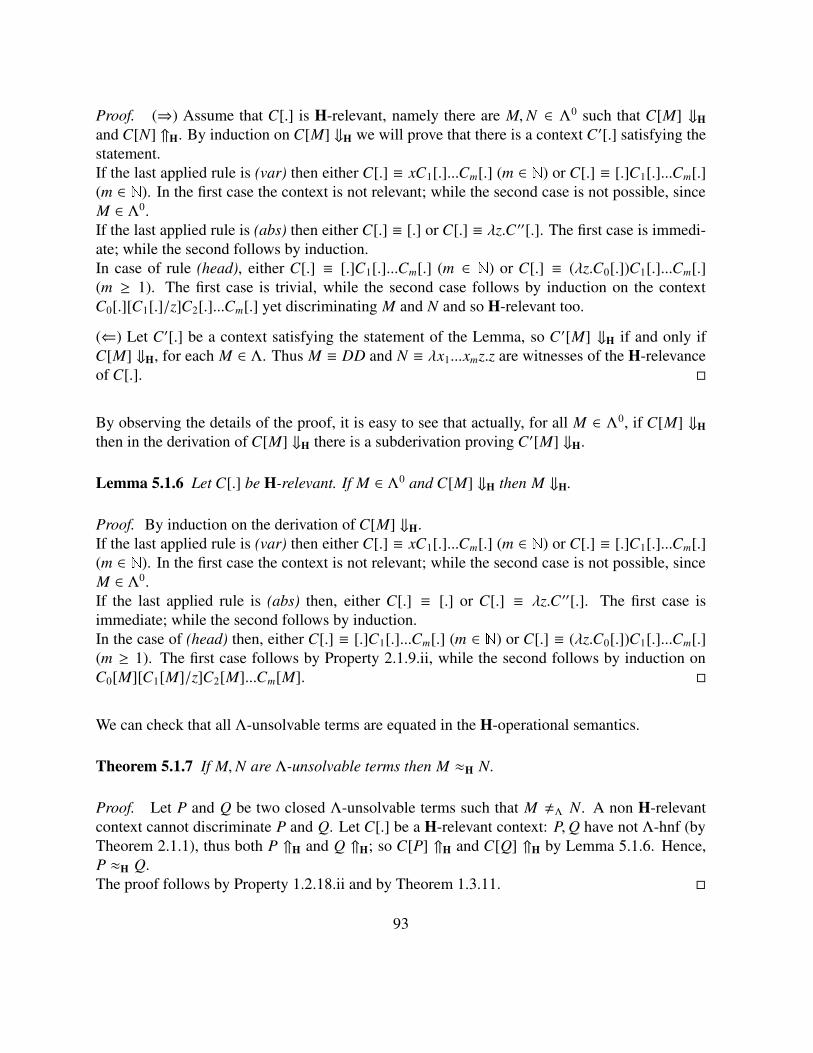
Proof. (⇒) Assume that C[.] is H-relevant, namely there are M,N ∈ Λ0 such that C[M] ⇓Hand C[N] ⇑H. By induction on C[M] ⇓H we will prove that there is a context C′[.] satisfying thestatement.If the last applied rule is (var) then either C[.] ≡ xC1[.]...Cm[.] (m ∈ ) or C[.] ≡ [.]C1[.]...Cm[.](m ∈

). In the first case the context is not relevant; while the second case is not possible, sinceM ∈ Λ0.If the last applied rule is (abs) then either C[.] ≡ [.] or C[.] ≡ λz.C ′′[.]. The first case is immedi-ate; while the second follows by induction.In case of rule (head), either C[.] ≡ [.]C1[.]...Cm[.] (m ∈

) or C[.] ≡ (λz.C0[.])C1[.]...Cm[.](m ≥ 1). The first case is trivial, while the second case follows by induction on the contextC0[.][C1[.]/z]C2[.]...Cm[.] yet discriminating M and N and so H-relevant too.

(⇐) Let C′[.] be a context satisfying the statement of the Lemma, so C ′[M] ⇓H if and only ifC[M] ⇓H, for each M ∈ Λ. Thus M ≡ DD and N ≡ λx1...xmz.z are witnesses of the H-relevanceof C[.].

By observing the details of the proof, it is easy to see that actually, for all M ∈ Λ0, if C[M] ⇓Hthen in the derivation of C[M] ⇓H there is a subderivation proving C′[M] ⇓H.

Lemma 5.1.6 Let C[.] be H-relevant. If M ∈ Λ0 and C[M] ⇓H then M ⇓H.

Proof. By induction on the derivation of C[M] ⇓H.If the last applied rule is (var) then either C[.] ≡ xC1[.]...Cm[.] (m ∈ ) or C[.] ≡ [.]C1[.]...Cm[.](m ∈

). In the first case the context is not relevant; while the second case is not possible, sinceM ∈ Λ0.If the last applied rule is (abs) then, either C[.] ≡ [.] or C[.] ≡ λz.C ′′[.]. The first case isimmediate; while the second follows by induction.In the case of (head) then, either C[.] ≡ [.]C1[.]...Cm[.] (m ∈

) or C[.] ≡ (λz.C0[.])C1[.]...Cm[.](m ≥ 1). The first case follows by Property 2.1.9.ii, while the second follows by induction onC0[M][C1[M]/z]C2[M]...Cm[M].

We can check that all Λ-unsolvable terms are equated in the H-operational semantics.

Theorem 5.1.7 If M,N are Λ-unsolvable terms then M ≈H N.

Proof. Let P and Q be two closed Λ-unsolvable terms such that M ,Λ N. A non H-relevantcontext cannot discriminate P and Q. Let C[.] be a H-relevant context: P,Q have not Λ-hnf (byTheorem 2.1.1), thus both P ⇑H and Q ⇑H; so C[P] ⇑H and C[Q] ⇑H by Lemma 5.1.6. Hence,P ≈H Q.The proof follows by Property 1.2.18.ii and by Theorem 1.3.11.

93

Thus the theory is sensible (see Definition 1.3.4).

Corollary 5.1.8 (H-incompleteness)The λ-calculus is incomplete with respect to the H-operational semantics.

Proof. Immediate, by Theorem 5.1.7.

The proof of the following property is an useful example of an useful technique for provingoperational equality between terms.

Property 5.1.9 I ≈H E.

Proof. By absurd assume that the two terms can be discriminated. This means that there is acontext C[.] discriminating them. Let C[.] be such that C[I] ⇓H while C[E] ⇑H. Clearly C[.]must be H-relevant.

Let C[.] be a minimal discriminating context for I and E, in the sense that the derivation ofC[I] ⇓H has a minimal size between all the proofs of C′[I] ⇓H, for every C′[.] discriminatingbetween I and E in such a way that C′[I] ⇓H while C′[E] ⇑H. The proof is done by consideringthe last applied rule in the derivation proving C[I] ⇓H.The last used rule cannot be (var), since C[.] ≡ xC1[.]...Cm[.] (m ∈

) is not H-relevant. Ifthe last used rule is (abs) then, either C[.] ≡ λx.C′[.] or C[.] ≡ [.]. In the former case, C′[.]would be a discriminating context such that the derivation of C′[I] ⇓H has smaller size than thederivation of C[I] ⇓H, against the hypothesis. The latter case is not possible, since clearly [.] isnot a discriminating context for I and E.Let the last used rule be (head), thus either C[.] ≡ (λx.C0[.])C1[.]...Cm[.] (m ≥ 1) or C[.] ≡[.]C1[.]...Cm[.] (m ∈

). Let consider the former case. By the rule (head), C[I] ⇓H if andonly if C0[I][C1[I]/x]C2[I]...Cm[I] ⇓H. But in this case C0[.][C1[.]/x]C2[.]...Cm[.] would be adiscriminating context C[.] for M and N with a derivation having smaller size than C[.], againstthe hypothesis that C[.] is minimum.The case C[.] ≡ [.]C1[.]...Cm[.] leads to a similar contradiction. In fact in this case C1[.]...Cm[.]would be a discriminating context “smaller” than C[.].The case C[I] ⇑H and C[E] ⇓H is symmetric.

Theorem 5.1.10 The theory H is fully extensional.

Proof. By Properties 2.1.7 and 5.1.9.

94

5.2 N-operational semantics

N ∈ E(Λ,Λ-NF) is the evaluation relation studied in this section; it is the universal evaluationrelationUΛ

Λ-NF.

In some sense, N induces the most natural operational semantics for the λΛ-calculus: in factconverging terms represent the completely terminating computations.

Definition 5.2.1 (N-operational semantics) i) N ∈ E(Λ,Λ-NF) is the evaluation relation in-duced by the formal system proving judgments of the shape

M ⇓N N

where M ∈ Λ and N ∈ Λ-NF. It consists of the following rules:

(Mi ⇓N Ni)(i≤m)(var)

xM1. . .Mm ⇓N xN1. . .Nm

M ⇓N N(abs)

λx.M ⇓N λx.N

P[Q/x]M1. . .Mm ⇓N N(head)

(λx.P)QM1. . .Mm ⇓N N

ii) M N N if and only if, for all context C[.] such that C[M],C[N] ∈ Λ0,(C[M] ⇓N implies

C[N] ⇓N).

iii) M ≈N N if and only if M N N and N N M.

As H, also the relation N is deterministic.

Example 5.2.2 λx1x2.x1(ID)((λuv.u)(II)x2) ⇓N λx1x2.x1DI, as shown by the following deriva-tion.

95

(var)x ⇓N x

(var)xx ⇓N xx

(abs)λx.xx ⇓N λx.xx

(head)ID ⇓N D

(var)x ⇓N x

(abs)λx.x ⇓N λx.x

(head)II ⇓N I

(abs)λv.II ⇓N λv.I

(head)(λuv.u)(II) ⇓N λv.I

(var)x1(ID)((λuv.u)(II)) ⇓N x1D(λv.I)

(abs)λx2.x1(ID)((λuv.u)(II)) ⇓N λx2.x1D(λv.I)

(abs)λx1x2.x1(ID)((λuv.u)(II)) ⇓N λx1x2.x1D(λv.I)

The system ⇓N characterizes completely, from an operational point of view, the class of Λ-normalforms.

Theorem 5.2.3 i) M ⇓N N implies M →∗pΛ

N and N is in Λ-nf.

ii) M ⇓N if and only if M has Λ-nf.

Proof.

i) By induction on the definition of ⇓N.

ii) (⇒) Directly from i).(⇐) If M →∗

ΛN ∈ Λ-NF then M →∗p

ΛN, by Corollary 1.2.13. The proof follows by

induction on the pair (M, p), where p is the length of the reduction sequence M →∗pΛ

Nordered in a lexicographic way.Let M ≡ λx1. . .xn.ζM1. . .Mm.If ζ is a variable then N ≡ λx1. . .xn.ζnfΛ(M1)...nfΛ(Mm). By induction Mi ⇓N (1 ≤ i ≤ m),thus M ⇓N by rule (var) having as premises the derivation proving Mi ⇓N and n instancesof (abs).If ζ ≡ (λx.P)Q then nfΛ(M) ≡ λx1. . .xn.nfΛ(P[Q/x]M1. . .Mm); so P[Q/x]M1. . .Mm ⇓N Rby induction, for some R; hence (λx.P)QM1. . .Mm ⇓N N, by applying rule (head) andM ⇓N λx1. . .xn.N by n instances of (abs).

An immediate consequence of the Theorem 5.2.3.ii is that M ⇓N implies M ⇓H.

Moreover, the λΛ-calculus is correct with respect to the N-operational semantics, as proved inthe following Theorem.

96

Theorem 5.2.4 (N-pretheory) N is a Λ-pretheory.

Proof. By Theorems 5.2.3 and 4.1.4.

We will prove that the λΛ-calculus is not complete with respect to the N-operational semantics,by using a syntactical characterization of N-relevant context.

Lemma 5.2.5 (N-relevance) A context C[.] is N-relevant if and only if there are n ≥ 1 contextsCi[.] ≡ [.]Ci

1[.]...Cimi

[.] (mi ∈ , 1 ≤ i ≤ n) such that for all M ∈ Λ0, C[M] ⇓N if and only if

∀i ≤ n, Ci[M] ⇓N.

Proof. (⇒) Assume that C[.] is N-relevant, namely there are M,N ∈ Λ0 such that C[M] ⇓N andC[N] ⇑N. By induction on C[M] ⇓N we will prove that there is at least one context satisfying thestatement.If the last applied rule is (var) then either C[.] ≡ xC1[.]...Cm[.] (m ∈ ) or C[.] ≡ [.]C1[.]...Cm[.](m ∈

). In the first case the N-relevance implies m ≥ 1, and C[M] ⇓N implies that C j[M] ⇓N,for each 1 ≤ j ≤ m. Let D1[.], ...Dh[.] (h ≤ m) be the subset of all relevant contexts inC1[.]...Cm[.]; it is not empty by the hypothesis tath C[.] is N-relevant. So the proof follows byinduction on contexts Di[.]. The second case is not possible, since M ∈ Λ0.If the last applied rule is (abs) then either C[.] ≡ [.] or C[.] ≡ λz.C ′′[.]. The first case is immedi-ate; while the second follows by induction.In the case of (head) then, either C[.] ≡ [.]C1[.]...Cm[.] (m ∈

) or C[.] ≡ (λz.C0[.])C1[.]...Cm[.](m ≥ 1). The first case is trivial, while the second case follows by induction on the contextC0[.][C1[.]/z]C2[.]...Cm[.] yet discriminating M and N and so N-relevant too.

(⇐) Let k = maxm1, ...,mn; it is easy to see that M ≡ DD and N ≡ λx1...xkz.z make C[.]relevant.

By observing the details of the proof, it is easy to see that actually, for all M ∈ Λ0, if C[M] ⇓Nthen in the derivation of C[M] ⇓N there are n subderivations proving C i[M] ⇓N (mi ∈ , 1 ≤ i ≤n).

The notion of N-relevant context is weaker than that one of H-relevant context. In particular, itdoes not enjoy of a property similar to that proved in the Lemma 5.1.6. Let C[.] ≡ [.](λx.I)(DD),so C[λxy.x(DD)] ⇓N I but λxy.y(DD) ⇑N; moreover C[λyx.x] ⇑N while λyx.x ⇓N.

So, in order to prove the operational equality between closed unsolvable terms, we will use a lessgeneral property of relevant contexts, but sufficient for our aim.

Lemma 5.2.6 Let C[.] be N-relevant. If M ∈ Λ0 and C[M] ⇓N then M is solvable.

97

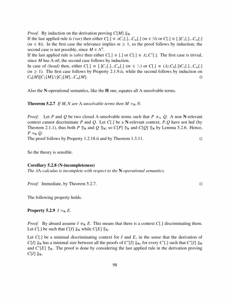
Proof. By induction on the derivation proving C[M] ⇓N.If the last applied rule is (var) then either C[.] ≡ xC1[.]...Cm[.] (m ∈ ) or C[.] ≡ [.]C1[.]...Cm[.](m ∈

). In the first case the relevance implies m ≥ 1, so the proof follows by induction; thesecond case is not possible, since M ∈ Λ0.If the last applied rule is (abs) then either C[.] ≡ [.] or C[.] ≡ λz.C ′[.]. The first case is trivial,since M has Λ-nf; the second case follows by induction.In case of (head) then, either C[.] ≡ [.]C1[.]...Cm[.] (m ∈

) or C[.] ≡ (λz.C0[.])C1[.]...Cm[.](m ≥ 1). The first case follows by Property 2.1.9.ii, while the second follows by induction onC0[M][C1[M]/z]C2[M]...Cm[M].

Also the N-operational semantics, like the H one, equates all Λ-unsolvable terms.

Theorem 5.2.7 If M,N are Λ-unsolvable terms then M ≈N N.

Proof. Let P and Q be two closed Λ-unsolvable terms such that P ,Λ Q. A non N-relevantcontext cannot discriminate P and Q. Let C[.] be a N-relevant context; P,Q have not hnf (byTheorem 2.1.1), thus both P ⇑N and Q ⇑N; so C[P] ⇑N and C[Q] ⇑N by Lemma 5.2.6. Hence,P ≈N Q.The proof follows by Property 1.2.18.ii and by Theorem 1.3.11.

So the theory is sensible.

Corollary 5.2.8 (N-incompleteness)The λΛ-calculus is incomplete with respect to the N-operational semantics.

Proof. Immediate, by Theorem 5.2.7.

The following property holds.

Property 5.2.9 I ≈N E.

Proof. By absurd assume I 0N E. This means that there is a context C[.] discriminating them.Let C[.] be such that C[I] ⇓N while C[E] ⇑N.

Let C[.] be a minimal discriminating context for I and E, in the sense that the derivation ofC[I] ⇓N has a minimal size between all the proofs of C′[I] ⇓N, for every C′[.] such that C′[I] ⇓Nand C′[E] ⇑N. The proof is done by considering the last applied rule in the derivation provingC[I] ⇓N.

98

If the last applied rule is (var) then C[.] ≡ xC1[.]...Cm[.] (m ∈ ), so there is a Ck[.] (1 ≤ k ≤ m)discriminating I and E with a derivation having smaller size, against the hypothesis that C[.] isminimum.If the last used rule is (abs) then, either C[.] ≡ λx.C ′[.] or C[.] ≡ [.]. In the former case, C′[.]would be a discriminating context such that the derivation of C′[I] ⇓N has smaller size than thederivation of C[I] ⇓N, against the hypothesis. The latter case is not possible, since clearly [.] isnot a discriminating context for I and E.Let the last used rule be (head), thus either C[.] ≡ (λx.C0[.])C1[.]...Cm[.] (m ≥ 1) or C[.] ≡[.]C1[.]...Cm[.] (m ∈ ). In the former case, the context C′[.] ≡ C0[.][C1[.]/x]C2[.]...Cm[.] wouldbe a discriminating context, such that the derivation C′[I] has smaller size than C[.], against thehypothesis that C[.] is minimum. The case C[.] ≡ [.]C1[.]...Cm[.] leads to a similar contradiction.In fact in this case C1[.]...Cm[.] would be a discriminating context “smaller” than C[.].The case C[I] ⇑N and C[E] ⇓N is symmetric.

The next theorem show that the N-operational semantics is fully-extensional (see Section 1.3).

Theorem 5.2.10 The theory ≈N is fully-extensional.

Proof. By Properties 2.1.7 and 5.2.9.

5.3 L-operational semantics

L ∈ E(Λ,Λ-LHNF) is the evaluation relation studied in this section; it is the universal evaluationrelationUΛ

Λ-LHNF.

The L-operational semantics models the so called lazy evaluation in a call by name parameterpassing environment: it is characterized by the fact that a Λ-redex is never reduced, in case itoccurs under the scope of an abstraction.

This behaviour is similar to that one of the real (call by name) programming languages, wherethe body of a procedure is evaluated only when its parameters are supplied.

Definition 5.3.1 (L-operational semantics) i) L ∈ E(Λ,Λ-LHNF) is the evaluation relationinduced by the formal system proving judgments of the shape

M ⇓L N

where M ∈ Λ and N ∈ Λ-LHNF. It consists of the following rules:

99

m ≥ 0(var)

xM1. . .Mm ⇓L xM1. . .Mm

(lazy)λx.M ⇓L λx.N

P[Q/x]M1. . .Mm ⇓L N(head)

(λx.P)QM1. . .Mm ⇓L N

ii) M L N if and only if, for all context C[.] such that C[M],C[N] ∈ Λ0,(C[M] ⇓L implies

C[N] ⇓L).

iii) M ≈L N if and only if M L N and N L M.

The formal system described before, when restricted to closed terms, corresponds to the call-by-name lazy evaluation machine introduced by Plotkin [81].

It is easy to check that L is deterministic.

Example 5.3.2 (λxy.x)(DD) ⇓L λy.DD. In fact we can build the following derivation:

(lazy)λy.DD ⇓L λy.DD

(head)(λxy.x)(DD) ⇓L λy.DD

The following theorem proves that the system L characterizes completely the class of Λ-lazyhead normal forms.

Theorem 5.3.3 i) M ⇓L N implies M →∗pΛ

N and N is in Λ-lhnf.

ii) M ⇓L if and only if M has a Λ-lhnf.

Proof.

i) By induction on the definition of ⇓L.

100

ii) (⇒) The proof is a consequence of i).(⇐) M has a Λ-lhnf means that there is N ∈ Λ-LHNF such that M =Λ N. But Λ-LHNF isa set of output value with respect to Λ, by Property 4.0.8; so there is a reduction sequenceM →∗p

ΛM′ ∈ Λ-LHNF.

The proof is done by induction on the length of the reduction sequence M →∗pΛ

M′. LetM ≡ λx1. . .xn.ζM1. . .Mm.If either n ≥ 1 or ζ is a variable, then a Λ-lhnf of M is M itself, so M ⇓L M, by anapplication of rule (lazy) or an application of rule (var).If n = 0 and ζ ≡ (λx.P)Q then the Λ-lhnf of M is a Λ-lhnf of P[Q/x]M1. . .Mm. Byinduction P[Q/x]M1. . .Mm ⇓L N, for some N, so M ⇓L N, by applying the rule (head).

By Theorem 5.3.3, it follows that both M ⇓H and M ⇓N imply M ⇓L. The following Lemmaproves that the λΛ-calculus is correct with respect to the L-operational semantics.

Theorem 5.3.4 (L-pretheory) ≈L is a Λ-pretheory.

Proof. By Theorems 5.3.3 and 4.1.4.

We will prove that the λΛ-calculus is not complete with respect to the L-operational semantics,by using a syntactical characterization of L-relevant context.

Lemma 5.3.5 (L-relevance) A context C[.] is L-relevant if and only if there is a context C ′[.] ≡[.]C1[.]...Cm[.] (m ∈ ) such that for all M ∈ Λ0, C[M] ⇓L if and only if C′[M] ⇓L.

Proof. (⇒) Assume that C[.] is L-relevant, namely there are M,N ∈ Λ0 such that C[M] ⇓Land C[N] ⇑L. By induction on C[M] ⇓L we will prove that there is a context C′[.] satisfying thestatement.The last applied rule cannot be (var), since C[.] ≡ xC1[.]...Cm[.] (m ∈

) is not relevant. If thelast applied rule is (lazy) then either C[.] ≡ [.] or C[.] ≡ λz.C ′′[.]. The first case is immediate;while the second is not possible, since λz.C′′[.] is not relevant.In the case of (head) then either C[.] ≡ [.]C1[.]...Cm[.] (m ∈

) or C[.] ≡ (λz.C0[.])C1[.]...Cm[.](m ≥ 1).The first case is trivial, while the second follows by induction on C0[.][C1[.]/z]C2[.]...Cm[.] yetdiscriminating M and N and so L-relevant too.

(⇐) Let C′[.] be a context satisfying the statement of the Lemma, so C ′[M] ⇓L if and only ifC[M] ⇓L, for each M ∈ Λ. Thus M ≡ DD and N ≡ λx1...xmz.z are witnesses of the L-relevanceof C[.].

101

By observing the details of the proof, it is easy to see that actually, for all M ∈ Λ, if C[M] ⇓L thenin the derivation of C[M] ⇓L there is a subderivation proving C′[M] ⇓L. Note that the contextλz.[.] is H-relevant but not L-relevant.

Lemma 5.3.6 Let C[.] be L-relevant. If M ∈ Λ0 and C[M] ⇓L then M ⇓L.

Proof. By induction on the derivation proving C[M] ⇓L.The last applied rule cannot be (var), since C[.] ≡ xC1[.]...Cm[.] (m ∈

) is not relevant. If thelast applied rule is (abs) then C[.] ≡ λz.C′[.] is not relevant, while the case C[.] ≡ [.] is trivial.In the case of (head) then, either C[.] ≡ [.]C1[.]...Cm[.] (m ∈

) or C[.] ≡ (λz.C0[.])C1[.]...Cm[.](m ≥ 1). The last case follows by induction on C0[M][C1[M]/z]C2[M]...Cm[M]; so let C[.] ≡[.]C1[.]...Cm[.] (m ∈

). If M ≡ λz.M′ then immediately M ⇓L, so let M ≡ (λz.P)QM1...Mn

(n ∈ ). C[M] ⇓L implies, by rule (head) that P[Q/z]M1...MnC1[M]...Cm[M] ⇓L.Since [.]C1[M]...Cm[M] is a relevant context (it discriminates DD and M), P[Q/z]M1...Mn ⇓L byinduction. Thus by applying the rule (head), M ⇓L follows.

An incompleteness result holds.

Theorem 5.3.7 (L-incompleteness)The λΛ-calculus is incomplete with respect to the L-operational semantics.

Proof. Let P and Q be two closed Λ-unsolvable terms of order zero such that P ,Λ Q. A nonL-relevant context cannot discriminate them. By Definition 2.1.3, if either P →∗

ΛR or Q →∗

ΛR,

for some R, then R cannot be an abstraction, hence P ⇑L and Q ⇑L. Let C[.] be any L-relevantcontext; so, by Lemma 5.3.6, C[P] ⇑L and C[Q] ⇑L. Hence, P ≈L Q.

Property 5.3.8 i) m , n implies λx1...xn.DD 0L λx1...xm.DD.

ii) I 0L E.

Proof.

i) Easy, by using the fact that DD ⇑L.

ii) The context [.](DD) discriminates the two given terms.

From the previous property and by Property 2.1.7, it follows that the operational semantics ≈L,being a Λ-theory, is not fully-extensional.

102

5.3.1 An example

We will show now that L0 ≈L L1, where

L0 ≡ λx.x(x(λx.DD)(DD))(λx.DD)L1 ≡ λx.x(λy.x(λx.DD)(DD)y)(λx.DD).

This equivalence has been firstly stated in [2], where it is showed that L0 and L1 are distinguishedby the interpretation in Scott-model considered in the paper.

First, let us prove a general property.

Lemma 5.3.9 Let M →∗η N. If N ⇓L then M ⇓L.

Proof. Let s be the size of the derivation proving N ⇓L and let l be the length of the reductionsequence from M to N. The proof is given by induction on the pair (s, l); the pairs are orderedaccording to the lexicographical order.If l = 0 then the proof is immediate, so let l ≥ 1.If N ≡ xN1...Nn (n ∈ ) then there are three cases.

1. M ≡ λy.M0y, where M0 →∗η N and y < FV(M0). The proof follows immediately by rule(lazy).

2. M ≡ (λy.M0y)M1...Mm (1 ≤ m ≤ n), where M0M1...Mm →∗η N and y < FV(M0). Byinduction M0M1...Mm ⇓L, hence M ⇓L by rule (head).

3. M ≡ xM1...Mn, where Mi →∗η Ni (1 ≤ i ≤ n). The proof follows by induction and by rule(var).

If N ≡ λx.N0 then M ≡ λy.M0 and the proof follows by rule (lazy). If N ≡ (λx.N0)N1...Nn

(n ≥ 1), then there are three cases.

1. M ≡ λy.M0y, where M0 →∗η N and y < FV(M0). The proof follows by rule (lazy).

2. M ≡ (λy.M0y)M1...Mm (1 ≤ m ≤ n), where M0M1...Mm →∗η N and y < FV(M0). Byinduction M0M1...Mm ⇓L, hence M ⇓L by rule (head).

3. M ≡ (λx.M0)M1...Mn, where Mi →∗η Ni (1 ≤ i ≤ n). It is easy to see that M0[M1/x]M2...Mn →∗ηN0[N1/x]N2...Nn. But N ⇓L implies N0[N1/x]N2...Nn ⇓L, and there is a derivation havingsize less than s proving it, hence by induction M0[M1/x]M2...Mn ⇓L. Then the proof fol-lows by rule (head).

103

The previous Lemma implies the following Corollary.

Corollary 5.3.10 If M →∗η N then N L M.

Proof. Clearly C[M] →∗η C[N], for all context C[.]. Then by Lemma 5.3.9, C[N] ⇓L impliesC[M] ⇓L.

In particular, it follows that L0 L L1. The next goal is to prove the reverse relation, namelyL1 L L0.

Let M ∈ Λ0; it is easy to check that M(λy.M(λx.DD)(DD)y)(λx.DD) ⇓L if and only if L1M ⇓L,by rule (head).

Lemma 5.3.11 Let M,N ∈ Λ0 be such that N =Λ M.If M(λy.N(λx.DD)(DD)y)(λx.DD) ⇓L, then either N →∗

Λλx0x1.x0 or N →∗

Λλx0x1.x1 or N →∗

Λ

λx0x1x2.M′′′, for some M′′′ ∈ Λ.

Proof. Let R ≡ M(λy.N(λx.DD)(DD)y)(λx.DD). The proof is by induction on the derivationproving R ⇓L.The last applied rule cannot be (var), since R ∈ Λ0. The last applied rule cannot be (lazy), sinceR is not an abstraction. Hence the last applied rule is (head); we consider all the possible shapesof M.

• M ≡ xM1...Mm (m ∈ ) is not possible, since M ∈ Λ0.

• M ≡ (λx0.M′)M1...Mm (m ≥ 1). The proof follows by induction on

M′[M1/x0]M2...Mm(λy.N(λx.DD)(DD)y)(λx.DD) ⇓L .

• Let M ≡ λx0.M′, so FV(M′) ⊆ x0.– M′ ≡ x0M1...Mm (m ∈ ) is not possible, in fact ≈L is a Λ-theory, so N(λx.DD)(DD) ≈L

M(λx.DD)(DD) ≈L (λx.DD)M′1...M

′m(DD), where M′

i ≡ Mi[λx.DD/x0] (1 ≤ i ≤ m),and this fact impliesM(λy.N(λx.DD)(DD)y)(λx.DD) ⇑L.

104

– Let M′ ≡ (λx1.M0)M1...Mm (m ≥ 1) and T ≡ λy.N(λx.DD)(DD)y, so there is aderivation d and a term R′ such that

d(··· )

(M0[M1/x1])[T/x0]M1[T/x0]...Mm[T/x0](λx.DD) ⇓L R′(head)

(λx1.M0[T/x0])M1[T/x0]...Mm[T/x0](λx.DD) ⇓L R′(head)

(λx0.(λx1.M0)M1...Mm)(λy.N(λx.DD)(DD)y)(λx.DD) ⇓L R′

hence the proof follows by induction on

d(··· )

(M0[M1/x1])[T/x0]M1[T/x0]...Mm[T/x0](λx.DD) ⇓L R′(head)

(λx0.(M0[M1/x1])M2...Mm)(λy.N(λx.DD)(DD)y)(λx.DD) ⇓L R′

– Let M′ ≡ λx1.M0. Since M ∈ Λ0, there are only three further cases.

1. M ≡ λx0x1.x0M1...Mm (m ∈ ). If m ≥ 1, then

N(λx.DD)(DD) ≈L (λx0x1.x0M1...Mm)(λx.DD)(DD) ≈L (λx.DD)M′1...M

′m

where M′i ≡ Mi[λx.DD/x0,DD/x1] (1 ≤ i ≤ m), because ≈L is a Λ-theory, hence

R ⇑L since

R ≈L (λx0x1.x0M1...Mm)(λy.(λx.DD)M1...Mmy)(λx.DD)

So let m = 0 and the proof is done.2. M ≡ λx0x1.x1M1...Mm (m ∈

); it is easy to see that m ≥ 1 implies R ⇑L. Thecase m = 0 is like te previous one.

3. The case M ≡ λx0x1x2.M′′′ is immediate.

By using the previous characterization we can prove that L1 L L0.

Lemma 5.3.12 Let C[.] be such that C[L0],C[L1] ∈ Λ0. If C[L1] ⇓L then C[L0] ⇓L.

Proof. The proof is given by induction the the size of C[L1] ⇓L, by considering the last appliedrule.

(var) It is not possible, since C[L1] ∈ Λ0.

105

(lazy) If C[.] ≡ [.] then the proof is trivial, since L0 ⇓L. If C[.] ≡ λz.C′[.] then the proof is trivial,since C[.] is not relevant.

(head) Either C[.] ≡ (λz.C0[.])C1[.]...Cm[.] or C[.] ≡ [.]C1[.]...Cm[.] (m ≥ 1). In the first case theproof follows by induction on the context C0[L1][C1[L1]/z]C2[L1]...Cm[L1].In the second case, the hypothesis that the last applied rule is (head) implies m ≥ 1, andthere is a derivation d and a term R such that

d(head)

C1[L1](λy.C1[L1](λx.DD)(DD)y)(λx.DD)C2[L1]...Cm[L1] ⇓L R(head)

L1C1[L1]...Cm[L1] ⇓L R

By inductive hypothesis,

C1[L0](λy.C1[L0](λx.DD)(DD)y)(λx.DD)C2[L0]...Cm[L0] ⇓L

so by Lemma 5.3.11, there are three possible cases.

1. If C1[L0]→∗Λλx0x1.x0 then it is easy to see that

C1[L0](λy.C1[L0](λx.DD)(DD)y)(λx.DD) =Λ λx.DD;

so m ≥ 2 is not possible. Let m = 1; so it is easy to see that

λy.C1[L0](λx.DD)(DD)y =Λ λx.DD =Λ C1[L0](λx.DD)(DD).

Hence C1[L0](C1[L0](λx.DD)(DD))(λx.DD) ⇓L, since ≈L is a Λ-theory. By rule(head), C[L0] ⇓L.

2. If C1[L1]→∗Λλx0x1.x1 then it is easy to see that

C1[L0](λy.C1[L0](λx.DD)(DD)y)(λx.DD) =Λ λx.DD;

so m ≥ 2 is not possible and we can assume m = 1.But C1[L1] →∗

Λλx0x1.x1 implies C1[L0]Q(λx.DD) =Λ λx.DD, for each Q ∈ Λ.

Hence C1[L0](C1[L0](λx.DD)(DD))(λx.DD) ⇓L, since ≈L is a Λ-theory. By rule(head), C[L0] ⇓L.

3. If C1[L0]→∗Λλx0x1x2.M′′′, for some M′′′ ∈ Λ, then

C1[L0](λy.C1[L0](λx.DD)(DD)y)(λx.DD)C2[L0]...Cm[L0] =Λ

C1[L0](λy.M′′′[λx.DD/x0,DD/x1, y/x2])(λx.DD)C2[L0]...Cm[L0] =Λ

C1[L0](C1[L0](λx.DD)(DD))(λx.DD)C2[L0]...Cm[L0].

Since ≈L is a λΛ-theory,

C1[L0](C1[L0](λx.DD)(DD))(λx.DD)C2[L0]...Cm[L0] ⇓L

and the proof follows by applying the rule (head).

106

Theorem 5.3.13 L1 ≈L L0.

Proof. By Corollary 5.3.10 and Lemma 5.3.12

107

Chapter 6

Call-by-value operational semantics

6.1 V-operational semantics

As proved in the Property 4.0.8, the set of Γ-lazy blocked normal forms (Γ-lbnf’s), namelyΓ-LBNF = λx.M | M ∈ Λ ∪ xM1...Mm | Mi ∈ Λ , m ∈ ∪ (λx.P)QM1...Mm | P,Mi ∈Λ , Q < Γ , Q ∈ Γ-LBNF , m ∈ , is a set of output values with respect to Γ. Notice thatΓ-LBNF0 = Γ0.

V ∈ E(Γ,Γ-LBNF) is the evaluation relation studied in this section, it is the universal evaluationrelationUΓ

Γ-LBNF.

This operational semantics models the call-by-value parameter passing together with lazy evalu-ation.

Definition 6.1.1 (V-operational semantics) i) V ∈ E(Γ,Γ-LBNF) is the evaluation relation in-duced by the formal system proving judgments of the shape

M ⇓V N

where M ∈ Λ and N ∈ Γ-LBNF. It consists of the following rules:

(var)xM1. . .Mm ⇓V xN1. . .Nm

(lazy)λx.M ⇓V λx.M

108

Q ⇓V Q′ Q′ ∈ Γ P[Q′/x]M1. . .Mm ⇓V N(head)

(λx.P)QM1. . .Mm ⇓V N

Q ⇓V Q′ Q′ < Γ(block)

(λx.P)QM1. . .Mm ⇓V (λx.P)Q′M1. . .Mm

ii) M V N if and only if, for all context C[.] such that C[M],C[N] ∈ Λ0,(C[M] ⇓V implies

C[N] ⇓V).

iii) M ≈V N if and only if M V N and N V M.

The formal system described before, when restricted to closed terms, corresponds to the S.E.C.D.machine introduced by Landin [59], and further studied by Plotkin [81].

Example 6.1.2 (λx.yx)(Ky) ⇓V y(λz.y). In fact we can build the following derivation:

(var)y ⇓V y

(lazy)λz.y ⇓V λz.y

(head)Ky ⇓V λz.y

(var)y(λz.y) ⇓V y(λz.y)

(head)(λx.yx)(Ky) ⇓V y(λz.y)

V is deterministic and it characterizes the set Γ-LBNF.

Theorem 6.1.3 i) M ⇓V N implies M →∗pΓ

N and N is in Γ-lbnf.

ii) M ⇓V if and only if M has a Γ-lbnf.

Proof.

i) By induction on the rules of ⇓V.

ii) (⇒) The proof is a consequence of i).(⇐) M has a Γ-lbnf means that there is N ∈ Γ-LBNF such that M →∗

ΓN. But Γ-LBNF is

a set of output value with respect to Γ, by Property 4.0.8; so there is a reduction sequenceM →∗p

ΓM′ ∈ Γ-LBNF.

Let M ≡ λx1...xn.ζM1...Mm; we reason by induction on the length of M →∗pΓ

M′. If n , 0then the proof follows by rule (lazy), so let n = 0. If ζ ∈ Var the proof follows by rule (var).Otherwise ζ ≡ (λz.P)Q; hence, if Q is Γ-valuable then the proof follows by induction andrule (head), otherwise it follows by induction and rule (block).

109

Let M ∈ Λ0; it is easy to check that M ⇓V if and only if there is P ∈ Λ such that M →∗Γ` λx.P.

The λΓ-calculus is correct with respect to the V-operational semantics, as proved in the followingtheorem.

Theorem 6.1.4 (V-pretheory) ≈V is a Γ-pretheory.

Proof. By Theorems 6.1.3 and 4.1.4.

The V-relevant contexts cannot be characterized by using contexts of the shape [.]C1[.]...Cm[.](m ∈

), as in the call by name operational settings; in fact [.](DD[.])I is not V-relevant, while(λxy.y)([.]I) is V-relevant. However, the following lemma establishes a negative characterization.

Lemma 6.1.5 (V-relevance) Let C[.] be not V-relevant and M ∈ Λ0.If C[M] ⇓V then there is a context C′[.] such that, ∀P ∈ Λ0 C[P] ⇓V C′[P]; moreover C′[P] ∈ Γ

if and only if C′[M] ∈ Γ.

Proof. By induction on C[M] ⇓V, so by cases on the last applied rule.

(var) If C[.] ≡ xC1[.]...Cm[.] (m ∈ ) then the proof is trivial and C′[.] ≡ C[.]. The case

C[.] ≡ [.]C1[.]...Cm[.] (m ∈ ) is not possible, since M ∈ Λ0

(lazy) The case C[.] ≡ [.] is not possible, since it is trivially V-relevant; while in case C[.] ≡λz.C′′[.], the proof is trivial.

(head) C[.] ≡ [.]C1[.]...Cm[.] (m ∈ ) is not possible, since C[M] ⇓V while C[DD] ⇑V thus

C[.] is V-relevant, against the hypothesis; so, let C[.] ≡ (λz.C0[.])C1[.]...Cm[.] (m ≥ 1). Ifthere is N ∈ Λ0 such that C1[N] ⇑V then C[N] ⇑V, by implying that C[.] is V-relevant,against the hypothesis. Hence C1[.] is not relevant and C1[M] ⇓V, thus by induction thereis D1[.] such that ∀P ∈ Λ0 C1[P] ⇓V D1[P] and D1[P] ∈ Γ if and only if D1[P] ∈Γ. By induction on C0[M][D1[M]/x]C2[M]...Cm[M] there is a context C′[.] such thatC0[N][D1[N]/x]C2[N]...Cm[N] ⇓V C′[N] and C′[N] ∈ Γ if and only if C′[M] ∈ Γ, forall N ∈ Λ0. The proof follows by rule (head).

(block) The case C[.] ≡ [.]C1[.]...Cm[.] (m ∈ ) is not possible, since it is V-relevant (as in the

previous case); so, let C[.] ≡ (λz.C0[.])C1[.]...Cm[.] (m ≥ 1). Clearly C1[.] is not relevantand C1[M] ⇓V, so by induction there is D1[.] such that ∀P ∈ Λ0 C1[P] ⇓V D1[P] andD1[P] < Γ. Let C′[.] ≡ (λz.C0[.])D1[.]C2[.]...Cm[.] and the proof follows easily.

110

We will prove that the λΓ-calculus is not complete with respect to the V-operational semantics,by using the notion of V-relevant context.

Lemma 6.1.6 Let C[.] be V-relevant. If M ∈ Λ0 and C[M] ⇓V then M ⇓V.

Proof. By induction on C[M] ⇓V, so by cases on the last applied rule.

(var) C[.] ≡ xC1[.]...Cm[.] (m ∈ ), is not V-relevant.

(lazy) C[.] ≡ λz.C′[.] is not V-relevant, while C[.] ≡ [.] is trivial.

(head) Let C[.] ≡ [.]C1[.]...Cm[.] (m ∈ ), so there are two cases:

1. if M ≡ λz.M′ then M ⇓V;

2. let M ≡ (λz.P)QM1...Mn (n ∈ ). C[M] ⇓V implies P[Q/z]M1...MnC1[M]...Cm[M] ⇓Vby rule (head); since [.]C1[M]...Cm[M] is a relevant context (it discriminates M andDD), by induction P[Q/z]M1...Mn ⇓V. Thus by rule (head), it follows that M ⇓V.

Let C[.] ≡ (λz.C0[.])C1[.]...Cm[.] (m ≥ 1) so there two cases again:

1. if C1[.] is not relevant then there exists C′1[.] satisfying the Lemma 6.1.5, thus byinduction on C0[M][C′1[M]/z]C2[M]...Cm[M] ⇓L, the proof follows;

2. otherwise C1[.] is relevant and the proof follows by induction on C1[M] ⇓L.

(block) Let C[.] ≡ [.]C1[.]...Cm[.] (m ∈ ); if M ≡ (λx.P)QN1...Nn (n ∈

) then Q ⇓V Q′, butQ ∈ Λ0 and Q′ is a closed Γ-lbnf imply that Q′ is an abstraction, against the hypothesisthat the last applied rule is (block); thus M ≡ λx.M′ and M ⇓V by rule (lazy).Let C[.] ≡ (λz.C0[.])C1[.]...Cm[.] (m ≥ 1), so C1[.] is relevant and the proof follows byinduction.

The following result holds.

Theorem 6.1.7 (V-incompleteness)The λΓ-calculus is incomplete with respect to the V-operational semantics.

111

Proof. Let P and Q be two closed Γ-unsolvable terms of order zero such that P ,Λ Q. A nonV-relevant context cannot discriminate them. By Definition 3.1.12, if P →∗

ΓR or Q →∗

ΓR, for

some R, then R cannot be an abstraction, hence P ⇑V and Q ⇑V. Let C[.] be a V-relevant context;so, by Lemma 6.1.6, C[P] ⇑V and C[Q] ⇑V. Hence, P ≈V Q.

As corollary, we obtain that the V-operational equivalence equates all closed Γ unsolvable termsof the same order.

Corollary 6.1.8Let P and Q be closed Γ-unsolvable terms of the same order n. Then P ≈V Q.

Proof. By induction on n. If n = 0, then the proof follows from the proof of the incompletenessresult. Otherwise it follows by induction.

The next property shows an interesting characterization of the V-operational semantics.

Property 6.1.9 Let M and N be such that M is potentially Γ-valuable while N is not potentiallyΓ-valuable. Then M 0V N.

Proof. According to the definition of potentially Γ-valuable term, we will consider only sub-stitutions whose codomain is Γ. M potentially Γ-valuable means that there is a substitutions such that s(M) ∈ Λ0 is Γ-valuable, while s′(N) is not Γ-valuable, for each substitution s′such that s′(N) ∈ Λ0. So let s be such that s(M) is Γ-valuable: we can easily extend s to asubstitution s′ such that s′(M) ∈ Λ0 is Γ-valuable while s′(N) ∈ Λ0 is not Γ-valuable. LetC[.] ≡ (λx1...xn.[.])s′(x1)...s′(xn) where FV(M) ∪ FV(N) ⊆ x1, ..., xn; it is easy to see that C[.]is discriminating for M and N.

The V-theory is not fully extensional. In fact, DD 0V λx.DDx.

6.1.1 An example

We will show now that V0 ≈V V1, where

V0 ≡ λx.(λx1x2.DD)(x(λx1.DD)(λx1.DD))V1 ≡ λx.(λx1x2x3.DD)(x(λx1.DD)(λx1x2.DD))(x(λx1x2.DD)(λx1.DD)).

This equivalence has been firstly proved in [32], where it is showed that the two terms are dis-criminated by the interpretation in Scott-model considered in the paper.

The interest of such a result will be clear when we will study the denotational semantics.

112

Lemma 6.1.10 Let M ∈ Λ0.

i) If V0M ⇓V then V0M ⇓V (λx.DD).

ii) If V1M ⇓V then V1M ⇓V (λx.DD).

Proof. By Lemma 6.1.3, P ∈ Λ0 and P ⇓V P′ imply P′ is an abstraction.

i) Let D1 ≡ (λx1.DD) and D2 ≡ (λx1x2.DD); thus

d0·········

M ⇓V M0

d1·········

M0D1D1 ⇓V M1

(lazy)λx2.DD ⇓V λx2.DD

(head)(λx1x2.DD)(M0D1D1) ⇓V λx2.DD

(head)(λx.D2(xD1D1))M ⇓V λx2.DD

ii) Let D1 ≡ (λx1.DD), D2 ≡ (λx1x2.DD) and D3 ≡ (λx1x2x3.DD); thus

d0·········

M ⇓V M0

d1·········

M0D1D2 ⇓V M1

d1·········

M0D1D2 ⇓V M2

(lazy)λx.DD ⇓V λx.DD

(head)D2((M0D2D1) ⇓V λx.DD

(head)D3(M0D1D2)(M0D2D1) ⇓V λx.DD

(head)(λx.D3(xD1D2)(xD2D1))M ⇓V λx.DD

Lemma 6.1.11 Let C[.] be a context such that C[V0],C[V1] ∈ Λ0.

i) If C[V0] ⇓V then ∃C′[.] such that C[V0] ⇓V C′[V0] and C[V1] ⇓V C′[V1].

ii) If C[V1] ⇓V then ∃C′[.] such that C[V0] ⇓V C′[V0] and C[V1] ⇓V C′[V1].

Proof.

i) By induction on the derivation proving C[V0] ⇓V.

(var) This case is not possible, since by hypothesis C[V0] ∈ Λ0.

113

(lazy) C[.] ≡ λz.C0[.] and C[.] ≡ [.] are both trivial.

(head) Let C[.] ≡ [.]C1[.]...Cm[.] (m ≥ 1); if m ≥ 2 then by Lemma 6.1.10 it is easy tosee that C[V0] ⇑V, so let m = 1. The proof follows by Lemma 6.1.10. Let C[.] ≡(λz.C0[.])C1[.]...Cm[.] (m ≥ 1), so by induction on C1[V0] ⇓V there is C′1[.] suchthat C1[V0] ⇓V C′1[V0] and C1[V1] ⇓V C′1[V1]. The proof follows by induction onC0[V0][C′1[V0]/z]C2[V0]...Cm[V0].

(block) This case is not possible, since by hypothesis C[V0] ∈ Λ0.

ii) (var) This case is not possible, since by hypothesis C[V0] ∈ Λ0.

(lazy) C[.] ≡ λz.C0[.] and C[.] ≡ [.] are both trivial.

(head) Let C[.] ≡ [.]C1[.]...Cm[.] (m ≥ 1), if m ≥ 2 then by Lemma 6.1.10 it is easyto see that C[V0] ⇑V, so let m = 1. The proof follows by Lemma 6.1.10. LetC[.] ≡ (λz.C0[.])C1[.]...Cm[.] (m ≥ 1) so by induction on C1[V1] ⇓V there is C′1[.]such that C1[V0] ⇓V C′1[V0] and C1[V1] ⇓V C′1[V1]. The proof follows by inductionon C0[V1][C′1[V1]/z]C2[V1]...Cm[V1].

(block) This case is not possible, since by hypothesis C[V0] ∈ Λ0.

Theorem 6.1.12 V0 ≈L V1.

Proof. The proof follows from Lemma 6.1.11.

114

Chapter 7

Operational Theories

7.1 Operational semantics and extensionality

In the Section 1.3, the notion of full extensionality has been introduced. A ∆-theory T is fully-extensional when all terms in it can be interpreted as functions, i.e., if and only if the full-extensionality principle holds:

(EXT) Mx =T Nx⇒ M =T N x < FV(M) ∪ FV(N).

Moreover we proved that a ∆-theory T is fully-extensional if and only if it is closed under η-equality, which is the congruence relation induced by the η-reduction rule:

(η) λx.Mx→η M if and only if x < FV(M).

Now the notion of extensionality will be considered in the particular setting of the ∆-theories,following the work done in [88].

Let O ∈ E(∆,Θ); intuitively a term M has a functional behaviour in O, or equivalently it canbe interpreted as a function, when M ≈O λx.Mx (x < FV(M)). If all terms have a functionalbehaviour in O, then it is natural to expect that ≈O in its turn behaves like the extensional equiv-alence on functions, i.e., if ∀P ∈ Λ, MP ≈O NP then M ≈O N. But not all operational theoriesgive a functional interpretation to all terms.

Let us consider, for example, the L-operational theory: DD and λx.DD have the same applicativebehaviour (since, for all y ∈ Var, both DDy ⇑L and (λx.DDx)y ⇑L), nevertheless they cannot beequated, since the context [.] separates them. In some sense DD, in the L-operational theory,can be see as a function too, but of arity 0. But the extensionality principle becomes vacuous ifextended to 0-arity functions. So we will introduce the notion of operational extensionality.

115

In order to formalize such a notion, let us introduce the key notion of O-comparable terms, withrespect to an operational theory O.

Definition 7.1.1 Let O ∈ E(∆,Θ) be defined by a formal system.M and N are O-comparable (notation M _O N) when, for each substitution s : Var → ∆ suchthat s(M), s(N) ∈ Λ0

s(M) ⇓O if and only if s(N) ⇓O.

Otherwise, M and N are said O-uncomparable (notation M ^O N).

We will speak simply about comparable terms if the involved operational semantics is clear bythe context.

Note that to be O-comparable does not imply to be equivalent. Let us consider the two termsλx.xzI and λx.xzO; if O ∈ H,N,L,V then λx.xzI _O λx.xzO but λx.xzI 0O λx.xzO. Notethat, x(DD) _V (λy.xy)(DD) are V-comparable although x(DD) ⇓V and (λy.xy)(DD) ⇑V.

To be comparable in a given operational semantics, is a necessary condition for two terms forbeing equivalent.

In the rest of this section, λ∗x.Mx will denote the fact that x < FV(M). Now we can state formallythe operational functionality principle.

(OP-FUN) O ∈ E(∆,Θ) is op-functional if and only if,for all M ∈ Λ, M _O λ∗x.Mx implies M ≈O λ∗x.Mx.

It is easy to see that M ≈O λ∗x.Mx implies M _O λ∗x.Mx.

Informally, an operational theory O is op-extensional when, for all terms M and N, if they canbe interpreted as functions and they have the same applicative behaviour, then M ≈O N.

(OP-EXT) O ∈ E(∆,Θ) is op-extensional if and only if,for all M,N ∈ Λ, for all x < FV(M) ∪ FV(N),if M _O λ∗x.Mx, N _O λ∗x.Nx and Mx ≈O Nx then M ≈O N.

It is easy to check that the two principles are equivalent when the operational semantics arecorrect.

Property 7.1.2 OP-FUN if and only if OP-EXT.

116

Proof. (⇒) Let O ∈ E(∆,Θ) satisfy OP-FUN. For all x < FV(M) ∪ FV(N), let M _O λ∗x.Mx,N _O λ∗x.Nx and Mx ≈O Nx.OP-FUN implies both M ≈O λ∗x.Mx and N ≈O λ∗x.Nx. Moreover λx∗.Mx ≈O λ∗x.Nx, sinceMx ≈O Nx and ≈O is a congruence; thus

M ≈O λ∗x.Mx ≈O λ∗x.Nx ≈O N.

(⇐) Let O ∈ E(∆,Θ) satisfying OP-EXT; let M _O λ∗x.Mx.Mz ≈O (λ∗x.Mx)z and λ∗x.Mx ≈O λ∗u.(λ∗x.Mx)u, since ≈O is a ∆-theory; thus, λ∗x.Mx _Oλ∗u.(λ∗x.Mx)u and by OP-EXT, M ≈O λ∗x.Mx.

The notion of op-extensionality can be captured by a suitable reduction rule, parameterized withrespect to the considered operational semantics.

Definition 7.1.3 Let O ∈ E(∆,Θ) be an evaluation relation.

i) The Oη-reduction (→Oη) is the contextual closure of the following rule: λ∗x.Mx →Oη M ifand only if M _O λ∗x.Mx;λ∗x.Mx is a Oη-redex and M is its contractum;

ii) M →∗Oη N and =Oη are respectively the reflexive and transitive closure of→Oη and the sym-metric, reflexive and transitive closure of→Oη.

iii) M →∆Oη N when either M →Oη N or M →∆ N;

iv) M →∗∆Oη N and =∆Oη are respectively the reflexive, symmetric and transitive of →∆Oη and

the symmetric, reflexive and transitive closure of→∆Oη.

A ∆-theory ≈O is a ∆Oη-theory, when ≈O is closed under =Oη, namely P =Oη Q implies P ≈O Q.

The relationship between op-extensionality and Oη-reduction rule is clarified in the next theorem.

Theorem 7.1.4 Let O ∈ E(∆,Θ) be correct with respect to the λ∆-calculus.O is op-extensional if and only if ≈O is closed under =Oη.

Proof.

⇒ Assume C[M] =Oη C[λ∗x.Mx], so M _O λ∗x.Mx by definition of→Oη.Clearly λ∗u.(λ∗x.Mx)u =∆ λ∗u.Mu, so λ∗u.(λ∗x.Mx)u ≈O λ∗u.Mu, since O is a ∆-theory,thus λ∗x.Mx _O λ∗u.(λ∗x.Mx)u too.Mz ≈O (λ∗x.Mx)z, since O is a ∆-theory. Hence M ≈O λ∗x.Mx by op-extensionality.Thus, C[M] ≈O C[λ∗x.Mx].

117

⇐ Let M _O λ∗x.Mx, N _O λ∗x.Nx and Mx ≈O Nx, for all x < FV(M) ∪ FV(N). Since Ois a ∆Oη-theory, both M ≈O λ∗x.Mx and N ≈O λ∗x.Nx. Moreover, Mx ≈O Nx implies(λ∗x.Mx) ≈O (λ∗x.Nx), so the proof follows by transitivity of ≈O.

We will prove that H, N, L and V are operationally extensional.

First we need to characterize the class of terms M such that M and λ∗x.Mx are O-comparable,when O ∈ H,N,L,V.

Lemma 7.1.5 Both M _H λ∗x.Mx and M _N λ∗x.Mx, for all M ∈ Λ.

Proof. Easy.

In H and N, the operational extensionality corresponds to full-extensionaly (see Theorems 5.1.10and 5.2.10).

Theorem 7.1.6 H and N are operational extensional Λ-theories.

Proof. Obvious, since fully-extensionality implies operational extensionality.

In L, it is no longer true that M _L λ∗z.Mz holds for all M ∈ Λ. In fact, y and λz.yz are notL-comparable (take the substitution s such that s(y) = DD).

Lemma 7.1.7M _L λ

∗z.Mz if and only if there is N ∈ Λ such that M →∗Λλx.N.

Proof.

⇒ Assume M does not reduce to an abstraction. This means that, for every reduction sequenceM →∗

ΛN, either N ≡ x ~Q or N ≡ U, where U is a Λ-unsolvable term of order 0. By

correctness, this implies either M ≈L x ~Q or M ≈L U. Let s be a substitution such thats(x) = DD, for all x.In both cases, s(x ~Q) and s(U) are Λ-unsolvable of order 0, hence s(x ~Q) ⇑L and s(U) ⇑L.On the other hand, s(λ∗z.Mz) =Λ λ∗z.s(M)z, so s(λ∗z.Mz) ⇓L, against the hypothesis thatM _L λ

∗z.Mz.

118

⇐ Let M →∗Λλx.N; so λ∗z.Mz →∗

Λλz.N[z/x], hence by correctness M ≈L λ∗z.Mz, which

implies M _L λ∗z.Mz.

By the previous lemma, the Lη-reduction (→Lη) can be restated, without any explicit referenceto the comparability relation L, as follows:

λ∗x.Mx→Lη M if and only if there is N ∈ Λ such that M →∗Λλx.N.

Theorem 7.1.8 L is an operational extensional Λ-theory.

Proof. By Lemma 7.1.7, if M =Lη N then M =Λ N, so M ≈L N by correctness and the prooffollows by Theorem 7.1.4.

Now let us consider the call-by-value operational semantics ≈V.

Lemma 7.1.9 M _V λ∗z.Mz if and only if M is Γ-valuable.

Proof.

(⇒) Assume that M →∗Γ

P implies P < Γ. This means that, for all reduction sequence M →∗Γ

N,either N ≡ x ~Q for some sequence ‖ ~Q‖ > 0, either N ≡ (λx.P)Q~R where Q < Γ, or N ≡ Uwhere U is a Γ-unsolvable term of order 0. Let s be a substitution such that ∀x ∈ Var,s(x) = λx.DD ∈ Γ.We prove by induction on N, that there is a substitution s such that s(N) ⇑V. The first andthe third case are obvious: both s(x ~Q) and s(U) are unsolvable of order 0, hence s(x ~Q) ⇑Vand s(U) ⇑V. In the second case, by induction s(Q) ⇑V; so, s((λx.P)Q~R) ⇑V. In all cases,s(M) ⇑V.On the other hand, s(λ∗z.Mz) = λ∗z.s(M)z, so s(λ∗z.Mz) ⇓V, against the hypothesis thatM _V λ

∗z.Mz.

(⇐) By definition, Γ = Var ∪ λx.M | M ∈ Λ. If M →∗Γλx.P′, for some P′, then M =Γ λ

∗z.Mz,so M ≈V λ∗z.Mz and M _V λ∗z.Mz. Let M →∗

Γx; for every substitution s : Var → Γ

such that s(M) ∈ Λ0, it is easy to see that s(x) ∈ Γ0 and M →∗Γ

x imply s(M) →∗Γ

s(x). Bycorrectness, s(M) ⇓V, while s(λ∗z.Mz) = λ∗z.s(M)z ∈ Γ0, so s(λ∗z.Mz) ⇓V. This implies,by definition, M _V λ

∗z.Mz.

119

By the previous lemma, the Vη-reduction (→Vη) can be restated, without any explicit referenceto the evaluation relation V, as follows:

λ∗x.Mx→Vη M if and only if M is Γ-valuable.

In the next chapter, we will prove that V is an operational extensional Γ-theory by using denota-tional tools.

An interesting overview on rewriting and extensionality can be found in [31].

7.2 Head-discriminability

We introduced in Definition 4.0.15, the notion of context discriminating a pair of terms, for agiven evaluation relation O. We will refine such a notion defining O head-discriminable, if theoperational difference between two terms can be tested through an head context. Clearly thisnotion is in some sense related to extensionality, since filling a head context C[.] by a closedterm M corresponds just to apply M to a suitable sequence of arguments.

Definition 7.2.1 O ∈ E(∆,Θ) is head discriminable if and only if C[M],C[N] ∈ Λ0 and C[M] ⇓Owhile C[N] ⇑O imply that there is a ∆-valuable head context C′[.] such that C′[M],C′[N] ∈ Λ0

and C′[M] ⇓O while C′[N] ⇑O (or viceversa).

Thus is a ∆-valuable head context is a context (λ~x[.])~P where P ∈ ~P is such that P ∈ ∆, byDefinitions 1.1.8 and 1.2.16.

Now let us define a particular class of operational semantics.

Definition 7.2.2An evaluation relation O is uniform if and only if λy.M ^O λx.N implies M ^O N.

Informally, the uniformity condition says that a reduction machine either computes under a λ-abstraction or not, in other words it has either a lazy or a not lazy behaviour, but it cannot mixthe two style of computing. Note that all the semantics we defined in this chapter are uniform.Moreover we would like to stress that uniformity is quite a natural property to expect for everyreasonable operational semantics.

120

It is easy to check that all the four operational semantics that we have studied are uniform.

We will prove in the next theorem that, for all the uniform operational semantics, head discrim-inability implies the operational extensionality.

Theorem 7.2.3If O ∈ E(∆,Θ) is uniform and head discriminable then it is operationally extensional.

Proof. Let O be head discriminable, M _O λ∗x.Mx and N _O λ∗x.Nx; we will prove thatM 0O N implies Mx 0O Nx, for all x < FV(M) ∪ FV(N).Since ≈O is head discriminable, M 0O N implies that there is a ∆-valuable head context (λ~y.[.])~Psuch that (λ~y.M)~P, (λ~y.N)~P ∈ Λ0, and (λ~y.M)~P ⇓O and (λ~y.N)~P ⇑O (or vice-versa).

• Let us consider the case ‖~P‖ = ‖~y‖. Thus M[~P/~y] ⇓O and N[~P/~y] ⇑O, by correctness.Since M _O λ∗x.Mx and N _O λ∗x.Nx, λ∗x.M[~P/~y]x ⇓O and λ∗x.N[~P/~y]x ⇑O. Thus thecontext (λ~yx.[.])~P discriminates Mx and Nx, which are so 0O.

• Let ‖~P‖ > ‖~y‖. Then ~P ≡ ~P1~P2, where ‖~P1‖ = ‖~y‖, and so M[~P1/~y]~P2 ⇓O and N[~P1/~y]~P2 ⇑O.But ‖~P2‖ > 0, ≈O is closed under =∆ and x < FV(M)∪FV(N), imply (λx.M[~P1/~y]x)~P2 ⇓Oand (λx.N[~P1/~y]x)~P2 ⇑O; thus by correctness, (λ~yx.Mx)~P1~P2 ⇓O and (λ~yx.Nx)~P1~P2 ⇑O.So the context (λ~yx.[.])~P1~P2 is a head context discriminating Mx and Nx, which are so 0O.

• Let ‖~P‖ < ‖~y‖. Then ~y ≡ ~y1~y2, where ‖~P‖ = ‖~y1‖, and, by ∆-reduction, λ~y2.M[~P/~y1] ⇓O andλ~y2.N[~P/~y1] ⇑O. By uniformity, this implies there is a substitution s such that s(M[~P/~y1]) ⇓Oand s(N[~P/~y1]) ⇑O, and consequently there is a substitution s′ such that s′(M) ⇓O ands′(N) ⇑O. Since M _O λ∗x.Mx and N _O λ∗x.Nx, λ∗x.s′(M)x ⇓O and λ∗x.s′(N)x ⇑O. LetC′[.] be the context such that, for all Q ∈ Λ, C′[Q] =∆ s′(Q). Then λx.C′[.] is the contextdiscriminating Mx and Nx, which are so 0O.

The previous theorem assures us that the notion of operational extensionality we defined is mean-ingful, under hypothesis of uniformity. In fact, head discriminability means that terms can bediscriminated just observing their applicative behaviour, so by considering them as functions,may be of arity 0.

All operational theories we considered are head-discriminable.

7.2.1 H is head-discriminable

Let M,N ∈ Λ0; we write M EH N in order to denote that M~P ⇓H imply N~P ⇓H, for each sequence~P of closed terms.

121

Theorem 7.2.4 Let M,N ∈ Λ0; M H N if and only if M EH N.

Proof. (⇒) Trivial.(⇐) We will show that C[M] ⇓H implies C[N] ⇓H; the proof is given by induction on the deriva-tion proving C[M] ⇓H.

(var) Clearly C[.] ≡ xC1[.]...Cm[.] (m ∈ ) thus the proof is trivial.

(abs) Either C[.] ≡ [.] or C[.] ≡ λx.C′[.]. In the first case the proof follows by hypothesis, in thesecond it follows by induction.

(head) There are two cases.

• Let C[.] ≡ [.]C1[.]...Cm[.] (m ∈ ) and let M ≡ (λz.M0)M1...Mn (n ∈ ) where m + n ≥ 1.If n = 0 then m ≥ 1, therefore we can let D[.] ≡ M0[C1[.]/z]C2[.]...Cm[.]; otherwise letD[.] ≡ M0[M1/z]M2...MnC1[.]...Cm[.]. In both cases D[M] ⇓H is the premise on the rule(head), so D[N] ⇓H by induction. Hence MC1[N]...Cm[N] ⇓H by rule (head), thus theproof follows by hypothesis.

• If C[.] ≡ (λx.C0[.])C1[.]...Cm[.] (m ≥ 1) then, since M ∈ Λ0, the proof follows by inductionon C[M] ≡ C0[M][C1[M]/x]C2[M]...Cm[M] ⇓H.

Hence, EH is a closed Λ-pretheory.

Corollary 7.2.5 H ∈ E(Λ,Λ-HNF) is head discriminable.

Proof. By Theorems 7.2.4 and 1.3.11, the proof follows.

7.2.2 N is head-discriminable

Let M,N ∈ Λ0; we write M EN N in order to denote that M~P ⇓N imply N~P ⇓N, for each sequence~P of closed terms.

Theorem 7.2.6 Let M,N ∈ Λ0; M N N if and only if M EN N.

122

Proof. (⇒) Trivial.(⇐) We will show that C[M] ⇓N implies C[N] ⇓N; the proof is given by induction on the deriva-tion proving C[M] ⇓N.All cases, but (var) are similar to that of the proof of the Lemma 7.2.4. If the last applied rule is(var) then C[.] ≡ xC1[.]...Cm[.] (m ∈ ), thus the proof follows by induction.

Hence, EN is a closed Λ-pretheory.

Corollary 7.2.7 N ∈ E(Λ,Λ-NF) is head discriminable.

Proof. By Theorems 7.2.6 and 1.3.11, the proof follows.

7.2.3 L is head-discriminable

Let M,N ∈ Λ0; we write M EL N in order to denote that M~P ⇓L imply N~P ⇓L, for each sequence~P of closed terms.

Theorem 7.2.8 Let M,N ∈ Λ0; M L N if and only if M EL N.

Proof. (⇒) Trivial.(⇐) We will show that if C[M],C[N] ∈ Λ0 then C[M] ⇓L implies C[N] ⇓L; the proof is given byinduction on the derivation proving C[M] ⇓L.

(var) It is not possible.

(lazy) Either C[.] ≡ [.] or C[.] ≡ λx.C′[.]. In the first case the proof follows by hypothesis whilethe second is trivial.

(head) There are two cases.

• Let C[.] ≡ [.]C1[.]...Cm[.] (m ∈ ) and let M ≡ (λz.M0)M1...Mn (n ∈ ) where m + n ≥ 1.If n = 0 then m ≥ 1, therefore we can let D[.] ≡ M0[C1[.]/z]C2[.]...Cm[.]; otherwise letD[.] ≡ M0[M1/z]M2...MnC1[.]...Cm[.]. In both cases D[M] ⇓L is the premise on the rule(head), so D[N] ⇓L by induction. Hence MC1[N]...Cm[N] ⇓L by rule (head), thus theproof follows by hypothesis.

• If C[.] ≡ (λx.C0[.])C1[.]...Cm[.] (m ≥ 1) then, since M ∈ Λ0, the proof follows by inductionon C[M] ≡ C0[M][C1[M]/x]C2[M]...Cm[M] ⇓L.

123

Hence, EL is a closed Λ-pretheory.

Corollary 7.2.9 L ∈ E(Λ,Λ-LHNF) is head discriminable.

Proof. By Theorems 7.2.8 and 1.3.11, the proof follows.

7.2.4 V is head-discriminable

A syntactical proof of the head-discriminability of the Γ-calculus is a little more complex, it willbe done by using the notion of weight (see Definition 3.1.29).

Let M,N ∈ Λ0; we write M EV N in order to denote that M~P ⇓V imply N~P ⇓V, for each sequence~P of closed terms.

Theorem 7.2.10 Let M,N ∈ Λ0; M V? N if and only if M EV N.

Proof. (⇒) Trivial, by Theorem 4.1.10.(⇐) Let C[M],C[N] ∈ Λ0 and note that Λ0 ∩ Γ-LBNF = Λ0 ∩ Ξ`-NF = Γ0.Clearly C[M] ⇓V if and only if C[M]→∗p

Γ?M′ ∈ Γ-LBNF if and only if C[M]→∗

Ξ` P ∈ Γ0 if andonly if C[M]→∗

Ξ` Q ∈ Ξ`-NF if and only if 〈C[M]〉 ∈ (by Corollary 3.2.2).We will show that 〈C[M]〉 ∈ implies 〈C[N]〉 ∈ . The proof is given by induction on 〈C[M]〉.〈C[M]〉 = 0 implies, either C[.] ≡ λx.C′[.] or C[.] ≡ [.]. In both case the proof is easy. Hence,let 〈C[M]〉 ≥ 1 and take in account the possible shape of contexts.

• If C[.] ≡ [.] then the proof is immediate by hypothesis.

• Let C[.] ≡ [.]C1[.]...Cm[.] (m ≥ 1) and let M ≡ (λz.M0).If D[.] ≡ M0[C1[.]/z]C2[.]...Cm[.] then 〈D[M]〉 < 1 + 〈C1[M]〉 + 〈D[M]〉 = 〈C[M]〉,therefore 〈D[M]〉 ∈

by induction. Moreover 〈C1[N]〉 ∈ by induction too. Hence

〈MC1[N]...Cm[N]〉 ∈ , so MC1[N]...Cm[N] ⇓V, by Corollary 3.2.2.Thus NC1[N]...Cm[N] ⇓V, by hypothesis and the proof follows by Corollary 3.2.2.

• Let C[.] ≡ [.]C1[.]...Cm[.] (m ≥ 1) and let M ≡ (λz.M0)M1...Mn (n ≥ 1).If D[.] ≡ M0[M1/z]M2...MnC1[.]...Cm[.] then 〈D[M]〉 < 〈C[M]〉, therefore 〈D[M]〉 ∈

by induction. Hence 〈MC1[N]...Cm[N]〉 ∈ , so MC1[N]...Cm[N] ⇓V, by Corollary 3.2.2.

Thus NC1[N]...Cm[N] ⇓V, by hypothesis and the proof follows by Corollary 3.2.2.

124

• If C[.] ≡ (λx.C0[.])C1[.]...Cm[.] (m ≥ 1) then 〈C0[M][C1[M]/x]C2[M]...Cm[M]〉 < 〈C[M]〉.Thus the proof follows by induction.

Hence, EV is a closed Γ-pretheory.

Corollary 7.2.11 V ∈ E(Λ,Λ-LBNF) is head discriminable.

Proof. The proof follows, by Theorems 7.2.10, 4.1.10 and 1.3.11.

We will show that the V-operational semantics is not semisensible (see Definition 1.3.4).

Theorem 7.2.12 The V-operational semantics is not semisensible.

Proof. Let YΓ be the recursion operator (λx f . f (λz.xx f z))(λx f . f (λz.xx f z)).Let B ≡ λxyz.x(yz), so clearly YΓB is an unsovale terms. By using the head discriminabilty it iseasy to check that YΓB ≈V I.

Let M ∈ Γ. It is easy to check that YΓBM ≈V IM ≈V M and that YΓBM is an unsolvable term.

125

Chapter 8

λ∆-Interaction Models

For studying the operational behaviour of λ-terms, usually a denotational (mathematical) ap-proach is followed. A denotational semantics for a language is based on the choice of a spaceof semantics values, or denotations, where terms are to be interpreted. Choosing a space withnice mathematical properties can help in proving semantic properties of terms, since to this aimstandard mathematical techniques can be used.

In the next definition, we will give the properties that a structure must satisfy in order to be usedas space of denotations for the λ∆-calculus, or, equivalently, to be a model for this calculus.

Definition 8.0.13 (λ∆-calculus model)A λ∆-model is a quadruple < , , , [[.]] >, where: is a set, is a map from 2 in and ⊆ . Moreover, if is the collection of functions(environments) from Var to , ranged over by ρ, ρ′, .., then the interpretation function [[.]] : Λ × → satisfies the following conditions:

1. [[x]]ρ = ρ(x);

2. [[MN]]ρ = [[M]]ρ [[N]]ρ;

3. [[λx.M]]ρ d = [[M]]ρ[d/x] if d ∈ ;4. if [[M]]ρ[d/x] = [[M′]]ρ′[d/y] for each d ∈ , then [[λx.M]]ρ = [[λy.M′]]ρ′;

5. M ∈ ∆ implies ∀ρ.[[M]]ρ ∈ .

where ρ[d/x](y) = if y ≡ x then d else ρ(y).

126

This definition assures that a λ∆-model respects some elementary key properties, namely theinterpretation of a term depends only on the behaviour of the environment on the free variables ofthe term itself, the α-rule is respected, the syntactical substitution is modeled by the environmentand the interpretation is contextually closed. Moreover is the semantical counterpart of the setof input values.

Property 8.0.14

i) If ρ(x) = ρ′(x), for all x ∈ FV(M), then [[M]]ρ = [[M]]ρ′ .

ii) If y < FV(M) then [[M]]ρ[d/x] = [[M[y/x]]]ρ[d/y], for all d ∈ .iii) If y < FV(M) then [[λx.M]]ρ = [[λy.M[y/x]]]ρ .

iv) If N ∈ ∆ then [[M[N/x]]]ρ = [[M]]ρ[[[N]]ρ/x] .

v) If [[M]]ρ = [[N]]ρ then, for every context C[.], [[C[M]]]ρ = [[C[N]]]ρ .

Proof.

i) By induction on M. If M ∈ Var then the proof is immediate. If M ≡ PQ then the prooffollows by induction and Definition 8.0.13.3. If M ≡ λx.N then by induction, ∀d ∈ ,[[N]]ρ[d/x] = [[N]]ρ′[d/x]; so [[λx.N]]ρ = [[λx.N]]ρ′ by Definition 8.0.13.4 .

ii) By induction on M. If M ∈ Var then the proof is immediate. If M ≡ PQ then the proof followsby induction. If M ≡ λz.N then by induction, ∀d′ ∈ , [[N]]ρ[d/x][d′/z] = [[N[y/x]]]ρ[d/y][d′/z]

(clearly ρ[d0/x0][d1/x1] = ρ[d1/x1][d0/x0]); hence, [[λz.N]]ρ[d/x] = [[(λz.N)[y/x]]]ρ′[d/y] byDefinition 8.0.13.4 and the proof is done.

iii) ∀d ∈ , [[M]]ρ[d/x] = [[M[y/x]]]ρ[d/y] by the previous point of this property. The proof followsby Definition 8.0.13.4 .

iv) By induction on M. If M ∈ Var then the proof is immediate. If M ≡ PQ then theproof follows by induction. If M ≡ λz.P then by induction ∀d ∈ , [[P[N/x]]]ρ[d/z] =

[[P]]ρ[d/z][[[N]]ρ[d/z]/x]; thus, [[M[N/x]]]ρ = [[M]]ρ[[[N]]ρ[d/z]/x] by Definition 8.0.13.4. Without lossof generality we can assume z < FV(N), hence [[M[N/x]]]ρ = [[M]]ρ[[[N]]ρ/x] by the point i)of this property.

v) By induction on the context C[.].If C[.] does not contains holes or C[.] ≡ [.], then the proof is obvious.If C[.] is C1[.]C2[.] then the proof follows immediately by induction.Let C[.] be λx.C′[.]; thus, ∀d ∈ , [[C′[M]]]ρ[d/x] = [[C′[N]]]ρ[d/x] by induction. The prooffollows by Definition 8.0.13.4 .

127

The previous property implies that Condition 3 of Definition 8.0.13 is the semantics counterpartof the ∆-reduction rule; it says that the interpretation of a term is closed under =∆, as proved inthe following.

Corollary 8.0.15 If M =∆ N, then [[M]]ρ = [[N]]ρ, for all ρ.

Proof. It is sufficient to prove that, if M →∆ N then [[M]]ρ = [[N]]ρ, for all ρ. Let Q ∈ ∆; so[[(λz.P)Q]]ρ = [[λz.P]]ρ [[Q]]ρ = [[P]]ρ[[[Q]]ρ/z] = [[P[Q/z]]]ρ by the definition of the model and byProperty 8.0.14.iv . The proof follows by Property 8.0.14.v .

Given a λ∆-model M, the interpretation function [[.]]M induces a denotational se-mantics on Λ. Namely two terms M and N are denotationally equivalent inM (andwe will write M ∼M N) if and only if:

[[M]]Mρ = [[N]]Mρ , for all environments ρ.

The Corollary 8.0.15 assure us that ∼M is a ∆-theory; moreover it implies that, if M =∆ N ∈ ∆

then ∀ρ.[[M]]ρ ∈ .

The denotational semantics induced by a model M is correct with respect to anoperational equivalence ≈O if:

M ∼M N implies M ≈O N, for all M and N;

while it is complete if:

M ≈O N implies M ∼M N, for all M and N.

A model is called fully-abstract with respect to an operational equivalence if theinduced denotational semantics is both correct and complete with respect to it.

The simplest denotational model is the so called term model.Let | M | be the ∆-equivalence class of M, i.e., | M |= N | N =∆ M; let | Λ | be the set all the

128

equivalence classes of Λ with respect to =∆, while | ∆ |⊆| Λ | is the set of equivalence classescontaining at least one input value.The term model TM(∆) is the quadruple <| Λ |, | ∆ |, , [[.]]TM(∆) >, where is defined as| M | | N |=| MN |.The interpretation of a term M in TM(∆), with FV(M) = x1,. . ., xm is given by [[M]]ρ =|M[N1/x1]..[Nm/xm] |, where Ni ∈ ρ(xi) (1 ≤ i ≤ m). It is easy to verify that TM(∆) satisfies theconditions of Definition 8.0.13.

Theorem 8.0.16 Let O be an evaluation relation.If the λ∆-calculus is correct w.r.t. ≈O then TM(∆) is correct for ≈O.

Proof. Since the λ∆-calculus is correct with respect to ≈O, =∆ implies ≈O. Since ∼TM (∆)coincide with =∆, the result follows.

It is easy to check that TM(Λ) is not complete with respect to the operational semantics H,N and L; while TM(Γ) is not complete with respect to the operational semantics V. Just taketwo unsolvable terms of order 0, e.g., DD and (λx.xxx)(λx.xxx). They are equated in all theoperational semantics above, while they are different in both TM(Λ) and TM(Γ).

Remark 8.0.17 The definition of λ∆-calculus model we gave, in case ∆ = Λ and = is thewell known definition of a λ-calculus model. But it looks different from the original one, given byHindley and Longo in [49]. In fact, they ask the interpretation function to satisfy the followingsix conditions:

1. [[x]]ρ = ρ(x);

2. [[MN]]ρ = [[M]]ρ [[N]]ρ;

3. [[λx.M]]ρ d = [[M]]ρ[d/x];

4. ρ(x) = ρ′(x) for all x ∈ FV(M)⇒ [[M]]ρ = [[M]]ρ′;

5. y < FV(M)⇒ [[λx.M]]ρ = [[λy.M[y/x]]]ρ;

6. if ∀d ∈ D[[M]]ρ[d/x] = [[M′]]ρ[d/x] then [[λx.M]]ρ = [[λx.M′]]ρ.

Our definition is shorter, and the strengthening of condition 4 allows to obtain, as side effect,both the α equality and the contextual equality (see Property 8.0.14).

129

8.1 Orthogonality

We will present now, a tentative of reinterpretation of some ludics idea [41, 43, 44] on the λ∆-calculus. Although clumsy in many sense, in this tentative we will show how beside the constuc-tion of a fully abstract model for a ∆-theory, there is some fine synthetic syntactical information(eventually infinitary). Therefore, we will propose a general setting where this kind of informa-tion can be considered.

As already said Λ0 has been defined as the set of closed λ-terms while ΛC has been defined asthe set of all contexts; we will use Λ0

C be the set of contexts C[.] such that P ∈ Λ0 implies thatC[P] ∈ Λ0 too.

Definition 8.1.1 A ∆-predicate P is simply a subset of Λ0 such that ∆-NF0 ⊆ P and M ∈ P andM =∆ N imply N ∈ P.

As example, you can put P be the set of closed terms having Λ-normal forms, or Λ-head normalforms, or Λ-weak head normal forms or again Γ-lazy blocked normal forms. The notion of ∆-predicate try to grasp the notion of closed output valuable terms; so it correspond to a restrictionof the notion of output valuable terms the defined in Subsection 4.1.1.

Property 8.1.2

i) If Θ is a set of output value with respect to ∆ then M ∈ Λ0 | M →∗∆

N ∈ Θ is a ∆-predicate.

ii) Let P be a ∆-predicate and ΘP = M ∈ Λ | FV(M) ⊆ x1, ..., xn implies λx1...xn.M ∈ P.If M ∈ P implies λx.M ∈ P, then ΘP is a set of output value with respect to ∆.

Proof.

i) Easy.

ii) Clearly ∆−NF ⊆ ΘP. Let M =∆ N ∈ ΘP and FV(M)∪FV(N) ⊆ x1, ..., xn. Thus λx1...xn.N ∈P by hypothesis, hence λx1...xn.M =∆ λx1...xn.N implies λx1...xn.M ∈ P. So M ∈ ΘP.

We will use A,B, ... in order to denote subsets of closed λ-terms and E,F , ... in order to denotesubsets of closing contexts.

130

Definition 8.1.3 Let P be a ∆-predicate,A ⊆ Λ0 and E ⊆ Λ0C.

A⊥⊥⊥⊥⊥⊥⊥⊥⊥ = C[.] ∈ Λ0C/∀M ∈ A s.t. C[M] ∈ P is said the set of orthogonal contexts of A with

respect to P. On the other hand, E>>>>>>>>> = M ∈ Λ0/∀C[.] ∈ E s.t. C[M] ∈ P the set of orthogonalterms of E with respect to P.( )>>>>>>>>> and ( )⊥⊥⊥⊥⊥⊥⊥⊥⊥ are said the pair of P-orthogonal operators.

℘(X) denote the powerset of a set X, namely the set A / A ⊆ X; thus ( )>>>>>>>>> is a function from℘(Λ0) to ℘(Λ0

C) while ( )⊥⊥⊥⊥⊥⊥⊥⊥⊥ is a function from ℘(Λ0C) to ℘(Λ0).

E⊥⊥⊥⊥⊥⊥⊥⊥⊥A (E are contexts for A) and A>>>>>>>>>E (A are terms for E) denote both A ⊆ E>>>>>>>>> and E ⊆ A⊥⊥⊥⊥⊥⊥⊥⊥⊥,that clearly are equivalent; namely E⊥⊥⊥⊥⊥⊥⊥⊥⊥A or A>>>>>>>>>E if and only if ∀M ∈ A ∀C[.] ∈ E C[M] ∈ Pwhere P is the corresponding ∆-predicate.

Let M be a closed λ-term; sometimes, by abusing the notation we will write M>>>>>>>>>C as an abbre-viation for M>>>>>>>>>C.

Property 8.1.4 Let P be a ∆-predicate,A ⊆ Λ0 and E ⊆ Λ0C.

A⊥⊥⊥⊥⊥⊥⊥⊥⊥>>>>>>>>> = M ∈ Λ0/∀C[.] ∈ Λ0C C[M] < P implies that ∃N ∈ A such that C[N] < P while

E>>>>>>>>>⊥⊥⊥⊥⊥⊥⊥⊥⊥ = C[.] ∈ Λ0C/∀M ∈ Λ0 C[M] < P implies that ∃C′[.] ∈ E such that C′[M] < P.

Proof. A⊥⊥⊥⊥⊥⊥⊥⊥⊥>>>>>>>>> = M ∈ Λ0/∀C[.] ∈ A⊥⊥⊥⊥⊥⊥⊥⊥⊥ C[M] ∈ P = M ∈ Λ0/∀C[.] (∀N ∈ A C[N] ∈ P) ⇒C[M] ∈ P = M ∈ Λ0/∀C[.] C[M] < P ⇒ (∃N ∈ A C[N] < P).By reasoning in the same way, the proof can be done for contexts.

For sake of simplicity, ( )>>>>>>>>> and ( )⊥⊥⊥⊥⊥⊥⊥⊥⊥ in what follows always will denote a pair of P-orthogonaloperators, for some ∆- predicate P.

Lemma 8.1.5 IfA ⊆ Λ0 and E ⊆ Λ0C thenA ⊆ A⊥⊥⊥⊥⊥⊥⊥⊥⊥>>>>>>>>> and E ⊆ E>>>>>>>>>⊥⊥⊥⊥⊥⊥⊥⊥⊥.

Proof. M ∈ A implies M>>>>>>>>>A⊥⊥⊥⊥⊥⊥⊥⊥⊥, so M ∈ A⊥⊥⊥⊥⊥⊥⊥⊥⊥>>>>>>>>>.C[.] ∈ E implies C[.]⊥⊥⊥⊥⊥⊥⊥⊥⊥E>>>>>>>>>, so C[.] ∈ E>>>>>>>>>⊥⊥⊥⊥⊥⊥⊥⊥⊥.

The next lemma shows that the orthogonality is antitone.

Lemma 8.1.6 i) IfA ⊆ B ⊆ Λ0 then B⊥⊥⊥⊥⊥⊥⊥⊥⊥ ⊆ A⊥⊥⊥⊥⊥⊥⊥⊥⊥.

ii) If E ⊆ F ⊆ Λ0C then F>>>>>>>>> ⊆ E>>>>>>>>>.

Proof.

131

i) C[.] ∈ B⊥⊥⊥⊥⊥⊥⊥⊥⊥ implies C[.]⊥⊥⊥⊥⊥⊥⊥⊥⊥B, thus C[.]⊥⊥⊥⊥⊥⊥⊥⊥⊥A i.e. C[.] ∈ A⊥⊥⊥⊥⊥⊥⊥⊥⊥.

ii) M ∈ E>>>>>>>>> implies M>>>>>>>>>E, thus M>>>>>>>>>F i.e. M ∈ F>>>>>>>>>.

Let A ⊆ B ⊆ Λ0. It is an easy corollary that A⊥⊥⊥⊥⊥⊥⊥⊥⊥>>>>>>>>> ⊆ B⊥⊥⊥⊥⊥⊥⊥⊥⊥>>>>>>>>>, therefore the biorthogonality ismonotone.

Lemma 8.1.7 IfA ⊆ Λ0 and E ⊆ Λ0C thenA⊥⊥⊥⊥⊥⊥⊥⊥⊥ = A⊥⊥⊥⊥⊥⊥⊥⊥⊥>>>>>>>>>⊥⊥⊥⊥⊥⊥⊥⊥⊥ and E>>>>>>>>> = E>>>>>>>>>⊥⊥⊥⊥⊥⊥⊥⊥⊥>>>>>>>>>.

Proof. A⊥⊥⊥⊥⊥⊥⊥⊥⊥ ⊆ (A⊥⊥⊥⊥⊥⊥⊥⊥⊥)>>>>>>>>>⊥⊥⊥⊥⊥⊥⊥⊥⊥ by Lemma 8.1.5. MoreoverA ⊆ A⊥⊥⊥⊥⊥⊥⊥⊥⊥>>>>>>>>> by Lemma 8.1.5, so (A⊥⊥⊥⊥⊥⊥⊥⊥⊥>>>>>>>>>)⊥⊥⊥⊥⊥⊥⊥⊥⊥ ⊆ A⊥⊥⊥⊥⊥⊥⊥⊥⊥by Lemma 8.1.6.E>>>>>>>>> ⊆ E>>>>>>>>>⊥⊥⊥⊥⊥⊥⊥⊥⊥>>>>>>>>> can be proved in a similar way.

Lemmas 8.1.5, 8.1.6, 8.1.7 say that biorthogonality is a closure operator, in the sense of thefollowing definition.

Definition 8.1.8 Let X be a set and let ℘(X) be its powerset.A function ˜ from ℘(X) to ℘(X) is said be a closing operator if and only if ∀A, B ⊆ X

• A ⊆ A

• A ⊆ B implies A ⊆ B

• ˜A ⊆ A.

Corollary 8.1.9 ( )⊥⊥⊥⊥⊥⊥⊥⊥⊥>>>>>>>>> and ( )>>>>>>>>>⊥⊥⊥⊥⊥⊥⊥⊥⊥ are closing operators.

Proof. By Lemmas 8.1.5, 8.1.6 and 8.1.7.

We call orthosets set of terms or contests that are closed by biorthogonality; furthermore Λ>>>>>>>>> andΛ⊥⊥⊥⊥⊥⊥⊥⊥⊥ will denote respectively A ⊆ Λ0 / ∃E ⊆ Λ0

C s.t. A = E>>>>>>>>> and E ⊆ Λ0C / ∃A ⊆ Λ0 s.t. E =

A⊥⊥⊥⊥⊥⊥⊥⊥⊥.

Lemma 8.1.10 i) IfA,B ⊆ Λ0 andA ⊆ B⊥⊥⊥⊥⊥⊥⊥⊥⊥>>>>>>>>> thenA⊥⊥⊥⊥⊥⊥⊥⊥⊥>>>>>>>>> ⊆ B⊥⊥⊥⊥⊥⊥⊥⊥⊥>>>>>>>>>.

ii) If E,F ⊆ Λ0C and E ⊆ F>>>>>>>>>⊥⊥⊥⊥⊥⊥⊥⊥⊥ then E>>>>>>>>>⊥⊥⊥⊥⊥⊥⊥⊥⊥ ⊆ F>>>>>>>>>⊥⊥⊥⊥⊥⊥⊥⊥⊥.

132

Proof.

i) By Lemma 8.1.6, (B⊥⊥⊥⊥⊥⊥⊥⊥⊥>>>>>>>>>)⊥⊥⊥⊥⊥⊥⊥⊥⊥ ⊆ A⊥⊥⊥⊥⊥⊥⊥⊥⊥ and (A⊥⊥⊥⊥⊥⊥⊥⊥⊥>>>>>>>>>) ⊆ (B⊥⊥⊥⊥⊥⊥⊥⊥⊥>>>>>>>>>)⊥⊥⊥⊥⊥⊥⊥⊥⊥>>>>>>>>>; but (B⊥⊥⊥⊥⊥⊥⊥⊥⊥>>>>>>>>>)⊥⊥⊥⊥⊥⊥⊥⊥⊥>>>>>>>>> = B⊥⊥⊥⊥⊥⊥⊥⊥⊥>>>>>>>>> by Lemma 8.1.7.

ii) Similar to the previous point.

8.2 Union and Intersection

Some interesting properties relates set theoretical intersection and union with>>>>>>>>> and⊥⊥⊥⊥⊥⊥⊥⊥⊥.

Lemma 8.2.1 i) If X ⊆ ℘(Λ0) then (⋃A∈XA)⊥⊥⊥⊥⊥⊥⊥⊥⊥ =

⋂A∈XA⊥⊥⊥⊥⊥⊥⊥⊥⊥.

ii) If X ⊆ ℘(Λ0C) then (

⋃E∈X E)>>>>>>>>> =

⋂E∈X E>>>>>>>>>.

Proof.

i) On the first hand, A ⊆ ⋃A∈XA for each A ∈ X, implies (

⋃A∈XA)⊥⊥⊥⊥⊥⊥⊥⊥⊥ ⊆ A⊥⊥⊥⊥⊥⊥⊥⊥⊥ by Lemma 8.1.6.

Thus (⋃A∈XA)⊥⊥⊥⊥⊥⊥⊥⊥⊥ ⊆ ⋂

A∈XA⊥⊥⊥⊥⊥⊥⊥⊥⊥.On the other hand, C[.] ∈ ⋂

A∈XA⊥⊥⊥⊥⊥⊥⊥⊥⊥ implies C[.] ∈ A⊥⊥⊥⊥⊥⊥⊥⊥⊥, for each A ∈ X; so C[.]⊥⊥⊥⊥⊥⊥⊥⊥⊥A, foreach A ∈ X thus C[.]⊥⊥⊥⊥⊥⊥⊥⊥⊥⋃

A∈XA and C[.] ∈ (⋃A∈XA)⊥⊥⊥⊥⊥⊥⊥⊥⊥.

ii) Similar to that of previous case.

In particular,A,B ⊆ Λ0 imply (A∪B)⊥⊥⊥⊥⊥⊥⊥⊥⊥ = A⊥⊥⊥⊥⊥⊥⊥⊥⊥∩B⊥⊥⊥⊥⊥⊥⊥⊥⊥, while E,F ⊆ Λ0C imply (E∪F )>>>>>>>>> = E>>>>>>>>>∩D>>>>>>>>>.

Furthermore,A,B ⊆ Λ0 impliesA⊥⊥⊥⊥⊥⊥⊥⊥⊥∪B⊥⊥⊥⊥⊥⊥⊥⊥⊥ ⊆ (A∩B)⊥⊥⊥⊥⊥⊥⊥⊥⊥ and E,F ⊆ Λ0C implies E>>>>>>>>>∪F>>>>>>>>> ⊆ (E∩F )⊥⊥⊥⊥⊥⊥⊥⊥⊥.

But the reverse inclusion is not always true.

Corollary 8.2.2 Λ>>>>>>>>> and Λ⊥⊥⊥⊥⊥⊥⊥⊥⊥ are closed under intersection.

Proof. We will show that, ifA,B ∈ Λ>>>>>>>>> thenA∩B ∈ Λ>>>>>>>>>.A = A⊥⊥⊥⊥⊥⊥⊥⊥⊥>>>>>>>>> and B = B⊥⊥⊥⊥⊥⊥⊥⊥⊥>>>>>>>>>, sinceA,B ∈ Λ>>>>>>>>>. ThusA∩B = A⊥⊥⊥⊥⊥⊥⊥⊥⊥>>>>>>>>> ∩B⊥⊥⊥⊥⊥⊥⊥⊥⊥>>>>>>>>> = (A⊥⊥⊥⊥⊥⊥⊥⊥⊥ ∪B⊥⊥⊥⊥⊥⊥⊥⊥⊥)>>>>>>>>> by Lemma8.2.1, so the proof follows by definition of Λ>>>>>>>>>. The same reasoning holds for Λ⊥⊥⊥⊥⊥⊥⊥⊥⊥.

A lemma on the possibility of “orthogonality-postposition” with respect to set theoretical unionfollows.

133

Lemma 8.2.3 i) If X ⊆ ℘(Λ0C) then (

⋃E∈X E>>>>>>>>>⊥⊥⊥⊥⊥⊥⊥⊥⊥)>>>>>>>>> = (

⋃E∈X E)>>>>>>>>>.

ii) If X ⊆ ℘(Λ0) then (⋃A∈XA⊥⊥⊥⊥⊥⊥⊥⊥⊥>>>>>>>>>)⊥⊥⊥⊥⊥⊥⊥⊥⊥ = (

⋃A∈XA)⊥⊥⊥⊥⊥⊥⊥⊥⊥.

Proof.

i) E ⊆ E>>>>>>>>>⊥⊥⊥⊥⊥⊥⊥⊥⊥ for each E ∈ X, implies⋃E∈X E ⊆

⋃E∈X E>>>>>>>>>⊥⊥⊥⊥⊥⊥⊥⊥⊥. Hence (

⋃E∈X E>>>>>>>>>⊥⊥⊥⊥⊥⊥⊥⊥⊥)>>>>>>>>> ⊆ (

⋃E∈X E)>>>>>>>>> by

Lemma 8.1.6.On the other hand, M ∈ (

⋃E∈X E)>>>>>>>>> implies M>>>>>>>>>⋃

E∈X E, thus M>>>>>>>>>E for each E ∈ X.Moreover M ∈ E>>>>>>>>> for each E ∈ X, thus M>>>>>>>>>E>>>>>>>>>⊥⊥⊥⊥⊥⊥⊥⊥⊥ for each E ∈ X. Therefore M>>>>>>>>>⋃

E∈X E>>>>>>>>>⊥⊥⊥⊥⊥⊥⊥⊥⊥,so M ∈ (

⋃E∈X E>>>>>>>>>⊥⊥⊥⊥⊥⊥⊥⊥⊥)>>>>>>>>>.

ii) Similar to that of previous case.

In particular, E,F ⊆ Λ0C imply (E ∪ F>>>>>>>>>⊥⊥⊥⊥⊥⊥⊥⊥⊥)>>>>>>>>> = (E ∪ F )>>>>>>>>> while A,B ⊆ Λ0 imply (A ∪ B⊥⊥⊥⊥⊥⊥⊥⊥⊥>>>>>>>>>)⊥⊥⊥⊥⊥⊥⊥⊥⊥ =

(A∪ B)⊥⊥⊥⊥⊥⊥⊥⊥⊥.

LetA,B ⊆ Λ0; thus (A∩B⊥⊥⊥⊥⊥⊥⊥⊥⊥>>>>>>>>>)⊥⊥⊥⊥⊥⊥⊥⊥⊥ ⊆ (A∩B)⊥⊥⊥⊥⊥⊥⊥⊥⊥, but the converse it is not true, in general.On the other hand E,F ⊆ Λ0

C implies (E ∩ F>>>>>>>>>⊥⊥⊥⊥⊥⊥⊥⊥⊥)>>>>>>>>> ⊆ (E ∩ F )>>>>>>>>>.

8.2.1 Orthogonal Lattices

Since orthosets are not closed under set-theoretical union, we will use ∪∗ in order to denote thebiorthogonal closure of an union.

Definition 8.2.4 i) IfA,B ⊆ Λ0 thenA∪∗B = (A∪B)⊥⊥⊥⊥⊥⊥⊥⊥⊥>>>>>>>>>.

ii) If E,F ⊆ Λ0C then E∪∗F = (E ∪ F )>>>>>>>>>⊥⊥⊥⊥⊥⊥⊥⊥⊥.

Note that the meaning of ∪∗ is overloaded.

Let X ⊆ ℘(Λ0) and Y ⊆ ℘(Λ0C), so

⋃∗A∈XA = (⋃A∈XA)⊥⊥⊥⊥⊥⊥⊥⊥⊥>>>>>>>>> while

⋃∗ E∈YE = (⋃E∈Y E)>>>>>>>>>⊥⊥⊥⊥⊥⊥⊥⊥⊥.

Theorem 8.2.5 i) Λ>>>>>>>>> endowed with ∩ and ∪∗ is a complete lattice.

ii) Λ⊥⊥⊥⊥⊥⊥⊥⊥⊥ endowed with ∩ and ∪∗ is a complete lattice.

Proof.

134

i) Let X ⊆ Λ>>>>>>>>> and B ∈ Λ>>>>>>>>>.If A ⊆ B for each A ∈ X, then

⋃A∈XA ⊆ B, thus (

⋃A∈XA)⊥⊥⊥⊥⊥⊥⊥⊥⊥>>>>>>>>> ⊆ B⊥⊥⊥⊥⊥⊥⊥⊥⊥>>>>>>>>> = B by Lemmas

8.1.6 and 8.1.7. Hence⋃∗A∈XA ⊆ B and

⋃∗A∈XA is the least upper bound (or supremum)of X.If B ⊆ A for each A ∈ X, then B ⊆ ⋂

A∈XA thus B = B⊥⊥⊥⊥⊥⊥⊥⊥⊥>>>>>>>>> ⊆ (⋂A∈XA)⊥⊥⊥⊥⊥⊥⊥⊥⊥>>>>>>>>> by Lemmas

8.1.6 and 8.1.7. But (⋂A∈XA)⊥⊥⊥⊥⊥⊥⊥⊥⊥>>>>>>>>> =

⋂A∈XA, so

⋂A∈XA is greatest lower bound (or

infimum) of X.

ii) Similar to that of the previous point.

Let A,B0,B1 ∈ Λ>>>>>>>>>. It is easy to see that (A ∩ B0) ∪ (A ∩ B1) = A ∩ (B0 ∪ B1), since thepowerset of a set is a distributive lattice; hence, (A∩B0)∪ (A∩B1) ⊆ A∩ (B0 ∪B1)⊥⊥⊥⊥⊥⊥⊥⊥⊥>>>>>>>>> implies((A∩B0) ∪ (A∩B1))⊥⊥⊥⊥⊥⊥⊥⊥⊥>>>>>>>>> ⊆ (A∩ (B0 ∪ B1)⊥⊥⊥⊥⊥⊥⊥⊥⊥>>>>>>>>>)⊥⊥⊥⊥⊥⊥⊥⊥⊥>>>>>>>>>. However, Λ>>>>>>>>> and Λ⊥⊥⊥⊥⊥⊥⊥⊥⊥ are not distributive.

As an example, let us consider the Λ-predicate PH = M ∈ Λ0 | M →∗∆

Λ-HNF.Let A = λx.xK(DD)⊥⊥⊥⊥⊥⊥⊥⊥⊥>>>>>>>>>, B0 = λx.xI(DD)⊥⊥⊥⊥⊥⊥⊥⊥⊥>>>>>>>>> and B1 = λx.x(DD)I⊥⊥⊥⊥⊥⊥⊥⊥⊥>>>>>>>>>. It is possible to showthat (B0 ∪ B1)⊥⊥⊥⊥⊥⊥⊥⊥⊥>>>>>>>>> = λx.x(DD)(DD)⊥⊥⊥⊥⊥⊥⊥⊥⊥>>>>>>>>>, but (A∩ B0)⊥⊥⊥⊥⊥⊥⊥⊥⊥>>>>>>>>> = ∅ and (A∩ B1)⊥⊥⊥⊥⊥⊥⊥⊥⊥>>>>>>>>> = λx.xKI⊥⊥⊥⊥⊥⊥⊥⊥⊥>>>>>>>>> (seeSection 8.6). So (A∩B0)∪(A∩B1) = λx.xKI⊥⊥⊥⊥⊥⊥⊥⊥⊥>>>>>>>>> whileA∩(B0∪B1)⊥⊥⊥⊥⊥⊥⊥⊥⊥>>>>>>>>> = λx.x(DD)(DD)⊥⊥⊥⊥⊥⊥⊥⊥⊥>>>>>>>>>.

8.3 Set applications

Definition 8.3.1 LetA,B ⊆ Λ0 and E,F ⊆ Λ0C. We define

A B = MN ∈ Λ0|M ∈ A ∧ N ∈ BE F = C[.] ∈ Λ0

C |C[E>>>>>>>>>[ ]] ⊆ F>>>>>>>>>⊥⊥⊥⊥⊥⊥⊥⊥⊥ ∧C[[ ]F>>>>>>>>>] ⊆ E>>>>>>>>>⊥⊥⊥⊥⊥⊥⊥⊥⊥

where

C[E>>>>>>>>>[ ]] = C′[ ] ∈ Λ0C |∃P ∈ E>>>>>>>>> C′[ ] ≡ C[P[ ]],

C[[ ]E>>>>>>>>>] = C′[ ] ∈ Λ0C |∃Q ∈ F>>>>>>>>> C′[ ] ≡ C[[ ]Q].

LetA,B ⊆ Λ0 and E,F ⊆ Λ0C.

SometimesA B will be denoted simplyAB; while EF will be used for E F .

Lemma 8.3.2 If E,F ⊆ Λ0C then E F = (E>>>>>>>>> F>>>>>>>>>)⊥⊥⊥⊥⊥⊥⊥⊥⊥.

135

Proof. Let ( )>>>>>>>>> and ( )⊥⊥⊥⊥⊥⊥⊥⊥⊥ be a pair of P-orthogonal operators.

C[.] ∈ E F ⇔

C[E>>>>>>>>>[ ]] ⊆ F>>>>>>>>>⊥⊥⊥⊥⊥⊥⊥⊥⊥ ⇔ C[E>>>>>>>>>F>>>>>>>>>] ∈ P ⇔ C[.]⊥⊥⊥⊥⊥⊥⊥⊥⊥E>>>>>>>>>F>>>>>>>>>

C[[ ]F>>>>>>>>>] ⊆ E>>>>>>>>>⊥⊥⊥⊥⊥⊥⊥⊥⊥ ⇔ C[B>>>>>>>>>F>>>>>>>>>] ∈ P ⇔ C[.]⊥⊥⊥⊥⊥⊥⊥⊥⊥E>>>>>>>>>F>>>>>>>>>

⇔ C[.] ∈ (E>>>>>>>>> F>>>>>>>>>)⊥⊥⊥⊥⊥⊥⊥⊥⊥.

Note that C[E>>>>>>>>>[ ]] ⊆ F>>>>>>>>>⊥⊥⊥⊥⊥⊥⊥⊥⊥ and C[[ ]F>>>>>>>>>] ⊆ E>>>>>>>>>⊥⊥⊥⊥⊥⊥⊥⊥⊥ conditions in definition are redundant.

By the previous Lemma E>>>>>>>>>F>>>>>>>>> ⊆ (E>>>>>>>>>F>>>>>>>>>)⊥⊥⊥⊥⊥⊥⊥⊥⊥>>>>>>>>> = (EF )>>>>>>>>>, but usually E>>>>>>>>>F>>>>>>>>> , (EF )>>>>>>>>>.In fact take in account the Λ-predicate PH of closed terms having head normal form: clearlyλx.xx⊥⊥⊥⊥⊥⊥⊥⊥⊥>>>>>>>>> , λx.xxx⊥⊥⊥⊥⊥⊥⊥⊥⊥>>>>>>>>>, but (λx.xxx)(λx.xxx) ∈ (λx.xx)(λx.xx)⊥⊥⊥⊥⊥⊥⊥⊥⊥>>>>>>>>> , λx.xx⊥⊥⊥⊥⊥⊥⊥⊥⊥>>>>>>>>> λx.xx⊥⊥⊥⊥⊥⊥⊥⊥⊥>>>>>>>>>.

A lemma on the postposition of orthogonality with respect to compositions.

Lemma 8.3.3 i) IfA,B ⊆ Λ0 then (A B⊥⊥⊥⊥⊥⊥⊥⊥⊥>>>>>>>>>)⊥⊥⊥⊥⊥⊥⊥⊥⊥ = (A B)⊥⊥⊥⊥⊥⊥⊥⊥⊥.

ii) If E,F ⊆ Λ0C then (E F>>>>>>>>>⊥⊥⊥⊥⊥⊥⊥⊥⊥) = (E F ).

Proof.

i) On a first hand,

A ⊆ AB ⊆ B⊥⊥⊥⊥⊥⊥⊥⊥⊥>>>>>>>>>

⇒A B ⊆ A B⊥⊥⊥⊥⊥⊥⊥⊥⊥>>>>>>>>> ⇒ (A B⊥⊥⊥⊥⊥⊥⊥⊥⊥>>>>>>>>>)⊥⊥⊥⊥⊥⊥⊥⊥⊥ ⊆ (A B)⊥⊥⊥⊥⊥⊥⊥⊥⊥.

On the other hand, C[.] ∈ (AB)⊥⊥⊥⊥⊥⊥⊥⊥⊥ ⇒ C[.]⊥⊥⊥⊥⊥⊥⊥⊥⊥(AB)⇒ C[A[ ]]⊥⊥⊥⊥⊥⊥⊥⊥⊥B ⇒ C[A[ ]] ⊆ B⊥⊥⊥⊥⊥⊥⊥⊥⊥ ⇒C[A[ ]]⊥⊥⊥⊥⊥⊥⊥⊥⊥B⊥⊥⊥⊥⊥⊥⊥⊥⊥>>>>>>>>> ⇒ C[.]⊥⊥⊥⊥⊥⊥⊥⊥⊥(A B⊥⊥⊥⊥⊥⊥⊥⊥⊥>>>>>>>>>)⇒ C[.] ∈ (A B⊥⊥⊥⊥⊥⊥⊥⊥⊥>>>>>>>>>)⊥⊥⊥⊥⊥⊥⊥⊥⊥.

ii) (E F>>>>>>>>>⊥⊥⊥⊥⊥⊥⊥⊥⊥) = (E>>>>>>>>> F>>>>>>>>>⊥⊥⊥⊥⊥⊥⊥⊥⊥>>>>>>>>>)⊥⊥⊥⊥⊥⊥⊥⊥⊥ = (E>>>>>>>>> F>>>>>>>>>)⊥⊥⊥⊥⊥⊥⊥⊥⊥ = E F by Lemma 8.3.2.

LetA ⊆ Λ0 and E ⊆ Λ0C. Note that (A⊥⊥⊥⊥⊥⊥⊥⊥⊥ E)>>>>>>>>> = (A⊥⊥⊥⊥⊥⊥⊥⊥⊥>>>>>>>>> E>>>>>>>>>)>>>>>>>>>⊥⊥⊥⊥⊥⊥⊥⊥⊥ = (A E>>>>>>>>>)⊥⊥⊥⊥⊥⊥⊥⊥⊥, by Lemma 8.3.2

and the first point of the previous Lemma.

Lemma 8.3.4 IfA,B0,B1 ⊆ Λ0 thenA (B0 ∪ B1) = AB0 ∪AB1

136

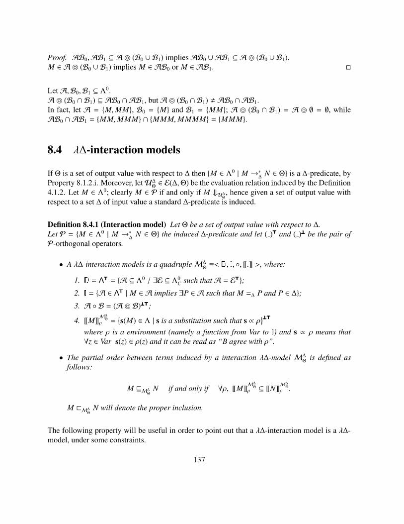
Proof. AB0,AB1 ⊆ A (B0 ∪ B1) impliesAB0 ∪AB1 ⊆ A (B0 ∪ B1).M ∈ A (B0 ∪ B1) implies M ∈ AB0 or M ∈ AB1.

LetA,B0,B1 ⊆ Λ0.A (B0 ∩ B1) ⊆ AB0 ∩AB1, butA (B0 ∩ B1) , AB0 ∩AB1.In fact, let A = M,MM, B0 = M and B1 = MM; A (B0 ∩ B1) = A ∅ = ∅, whileAB0 ∩AB1 = MM,MMM ∩ MMM,MMMM = MMM.

8.4 λ∆-interaction models

If Θ is a set of output value with respect to ∆ then M ∈ Λ0 | M →∗∆

N ∈ Θ is a ∆-predicate, byProperty 8.1.2.i. Moreover, letU∆

Θ∈ E(∆,Θ) be the evaluation relation induced by the Definition

4.1.2. Let M ∈ Λ0; clearly M ∈ P if and only if M ⇓U∆Θ, hence given a set of output value with

respect to a set ∆ of input value a standard ∆-predicate is induced.

Definition 8.4.1 (Interaction model) Let Θ be a set of output value with respect to ∆.Let P = M ∈ Λ0 | M →∗

∆N ∈ Θ the induced ∆-predicate and let ( )>>>>>>>>> and ( )⊥⊥⊥⊥⊥⊥⊥⊥⊥ be the pair of

P-orthogonal operators.

• A λ∆-interaction models is a quadrupleM∆Θ≡< , , , [[.]] >, where:

1. = Λ>>>>>>>>> = A ⊆ Λ0 / ∃E ⊆ Λ0C such thatA = E>>>>>>>>>;

2. = A ∈ Λ>>>>>>>>> | M ∈ A implies ∃P ∈ A such that M =∆ P and P ∈ ∆;3. A B = (A B)⊥⊥⊥⊥⊥⊥⊥⊥⊥>>>>>>>>>;

4. [[M]]M∆Θ

ρ =s(M) ∈ Λ | s is a substitution such that s ∝ ρ⊥⊥⊥⊥⊥⊥⊥⊥⊥>>>>>>>>>

where ρ is a environment (namely a function from Var to ) and s ∝ ρ means that∀z ∈ Var s(z) ∈ ρ(z) and it can be read as “B agree with ρ”.

• The partial order between terms induced by a interaction λ∆-model M∆Θ

is defined asfollows:

M vM∆Θ

N if and only if ∀ρ, [[M]]M∆Θ

ρ ⊆ [[N]]M∆Θ

ρ .

M @M∆Θ

N will denote the proper inclusion.

The following property will be useful in order to point out that a λ∆-interaction model is a λ∆-model, under some constraints.

137

Property 8.4.2 Let P be a ∆-predicate,A,B ⊆ Λ>>>>>>>>> and E ⊆ Λ⊥⊥⊥⊥⊥⊥⊥⊥⊥.

i) If M ∈ E>>>>>>>>> and M =∆ N then N ∈ E>>>>>>>>>.

ii) If ∀M ∈ A there is N ∈ B such that M =∆ N thenA⊥⊥⊥⊥⊥⊥⊥⊥⊥>>>>>>>>> ⊆ B⊥⊥⊥⊥⊥⊥⊥⊥⊥>>>>>>>>>.

iii) The orthosets induced from P are closed under =∆.

Proof.

i) Let M ∈ E>>>>>>>>> = M ∈ Λ0/∀C[.] ∈ E s.t. C[M] ∈ P; thus C[M] ∈ P and M =∆ N implyC[N] ∈ P, by Definition of ∆-predicate, so N ∈ E>>>>>>>>>.

ii) Since the Lemma 8.1.10, we will show simply thatA ⊆ B⊥⊥⊥⊥⊥⊥⊥⊥⊥>>>>>>>>>.Let M ∈ A, so by hypothesis there is N ∈ B such that M =∆ N. But N ∈ B⊥⊥⊥⊥⊥⊥⊥⊥⊥>>>>>>>>> by Lemma8.1.5, so M ∈ B⊥⊥⊥⊥⊥⊥⊥⊥⊥>>>>>>>>> by the previous point.

iii) Easy, by the previous points.

It is natural to ask that a not ∆-valuable term be different from a ∆-valuable term.

Definition 8.4.3A set Θ of output value with respect to ∆ is said strong if and only if M ∈ ∆0 and N < ∆0 implythat there is a context C[.] and a P ∈ Θ such that C[M] =∆ P, while C[N] ,∆ Q for each Q ∈ Θ.

The next theorem show that a λ∆-interaction model is a λ∆-model under hypothesis of uniformity(see Definition 7.2.2) and head discriminability (see Definition 7.2.1). Note that under thoseconditions an operational semantics is op-extensional.

Theorem 8.4.4 Let Θ be a set of strong output value with respect to ∆ and letM∆Θ≡< , , , [[.]] >

the induced λ∆-interaction model.IfU∆

Θ∈ E(∆,Θ) is uniform and head discriminable thenM∆

Θis a λ∆-model.

Proof.

1) [[x]]ρ = (ρ(x))⊥⊥⊥⊥⊥⊥⊥⊥⊥>>>>>>>>> = ρ(x) by Lemma 8.1.7.

138

2) [[MN]]M∆Θ

ρ =s(MN) ∈ Λ | s is a substitution such that s ∝ ρ⊥⊥⊥⊥⊥⊥⊥⊥⊥>>>>>>>>> =

s(M)s(N) ∈ Λ | s ∝ ρ⊥⊥⊥⊥⊥⊥⊥⊥⊥>>>>>>>>> = (((s(M) ∈ Λ | s ∝ ρ

s(N) ∈ Λ | s ∝ ρ)))⊥⊥⊥⊥⊥⊥⊥⊥⊥>>>>>>>>> =

(((s(M) ∈ Λ | s ∝ ρ⊥⊥⊥⊥⊥⊥⊥⊥⊥>>>>>>>>>

s(N) ∈ Λ | s is such that s ∝ ρ⊥⊥⊥⊥⊥⊥⊥⊥⊥>>>>>>>>>)))⊥⊥⊥⊥⊥⊥⊥⊥⊥>>>>>>>>> = [[M]]M∆Θ

ρ [[N]]M∆Θ

ρ

by Lemma 8.3.3.

3) IfA ∈ then [[λx.M]]M∆Θ

ρ A = ((([[λx.M]]M∆Θ

ρ A)))⊥⊥⊥⊥⊥⊥⊥⊥⊥>>>>>>>>> = (((s(λx.M) ∈ Λ | s ∝ ρ⊥⊥⊥⊥⊥⊥⊥⊥⊥>>>>>>>>> A)))⊥⊥⊥⊥⊥⊥⊥⊥⊥>>>>>>>>> =

(((s(λx.M) ∈ Λ | s ∝ ρA)))⊥⊥⊥⊥⊥⊥⊥⊥⊥>>>>>>>>> =

s((λx.M)N) ∈ Λ | s ∝ ρ and N ∈ A⊥⊥⊥⊥⊥⊥⊥⊥⊥>>>>>>>>> =

s(M[N/x]) ∈ Λ | s ∝ ρ and N ∈ A⊥⊥⊥⊥⊥⊥⊥⊥⊥>>>>>>>>> =

s′(M) ∈ Λ | s′ ∝ ρ[A/x]⊥⊥⊥⊥⊥⊥⊥⊥⊥>>>>>>>>> = [[M]]M

∆Θ

ρ[A/x]by Lemma 8.3.3 and by Property 8.4.2.

4) We will show that [[λx.M]]M∆Θ

ρ , [[λy.M′]]M∆Θ

ρ′ implies [[M]]M∆Θ

ρ[A/x] , [[M′]]M∆Θ

ρ′[A/y], for someA ∈ .s(λx.M) ∈ Λ | s ∝ ρ⊥⊥⊥⊥⊥⊥⊥⊥⊥>>>>>>>>> ,

s′(λy.M′) ∈ Λ | s′ ∝ ρ′⊥⊥⊥⊥⊥⊥⊥⊥⊥>>>>>>>>> impliess(λx.M) ∈ Λ | s ∝ ρ⊥⊥⊥⊥⊥⊥⊥⊥⊥ ,

s′(λy.M′) ∈ Λ | s′ ∝ ρ′⊥⊥⊥⊥⊥⊥⊥⊥⊥, by Lemma 8.1.6.Since the hypothesis of head discriminability, we can assume that there is a ∆-valuablehead context C[.] ≡ [.]P1...Pp (p ∈

), for some closed Pi ∈ ∆ (0 ≤ i ≤ p) such thatC[s(λx.M)] ∈ P for each s ∝ ρ while C[s′(λy.M′)] < P for some s′ ∝ ρ′ (or viceversa).If p = 0 then the proof follows by hypothesis of uniformity, so let p ≥ 1. If r ≡ s[P1/x] andr′ ≡ s′[P1/y] then r(M)P2...Pp ∈ P and r′(M′)P2...Pp < P, by Definition of ∆-predicate.Note that P⊥⊥⊥⊥⊥⊥⊥⊥⊥>>>>>>>>>1 ∈ , since Θ is strong and N ∈ P⊥⊥⊥⊥⊥⊥⊥⊥⊥>>>>>>>>>1 imply N =∆ Q ∈ ∆, and orthosets areclosed under =∆.Let A = P1⊥⊥⊥⊥⊥⊥⊥⊥⊥>>>>>>>>>, so

r(M) ∈ Λ | r ∝ ρ[A/x]

⊥⊥⊥⊥⊥⊥⊥⊥⊥ , r′(M′) ∈ Λ | r′ ∝ ρ′[A/y]

⊥⊥⊥⊥⊥⊥⊥⊥⊥; hencer(M) ∈ Λ | r ∝ ρ[A/x]

⊥⊥⊥⊥⊥⊥⊥⊥⊥>>>>>>>>> , r′(M′) ∈ Λ | r′ ∝ ρ′[A/y]

⊥⊥⊥⊥⊥⊥⊥⊥⊥>>>>>>>>> and [[M]]M∆Θ

ρ[A/x] , [[M′]]M∆Θ

ρ′[A/y].

5) M ∈ ∆ implies ∀ρ.[[M]]M∆Θ

ρ ∈ , since Θ is strong and the Property 8.4.2.

Let Θ be a set of strong output value with respect to ∆ and letM∆Θ≡< , , , [[.]] > the induced

λ∆-interaction model.IfU∆

Θ∈ E(∆,Θ) is uniform and head discriminable then it is easy to check that the denotational

equivalence ofM∆Θ

is fully abstract with respect to the corresponding universal operational se-mantics.

Theorem 8.4.5 (Full Abstraction) Let Θ be a set of strong output value with respect to ∆ in-ducing the λ∆-interaction model M∆

Θ≡< , , , [[.]] >. If U∆

Θ∈ E(∆,Θ) is uniform and head

discriminable then ∼M∆Θ

is fully abstract with respect to ≈U∆Θ.

Proof. Let M,N ∈ Λ0. It is immediate that M vM∆Θ

N if and only if M U∆Θ

N. Thus the prooffollows by the Lemma 1.3.11.

139

We have already noted that the four instances of studied operational semantics are uniform andhead-discriminable, moreover it is easy to see that their sets od output values are strong. Thus,for each one of they, the related interaction model is fully abstract.

8.5 Some further operations

For sake of simplicity, ( )>>>>>>>>> and ( )⊥⊥⊥⊥⊥⊥⊥⊥⊥ in what follows always will denote a pair of P-orthogonaloperators, for some ∆- predicate P.

Definition 8.5.1 LetA,B ⊆ Λ0. A ⇒ B is defined as the set M ∈ Λ0 | M A ⊆ B.

Some further ludics-style property of the structure can be showed.

Lemma 8.5.2 LetA,B ⊆ Λ0.

i) If B ∈ Λ>>>>>>>>> thenA ⇒ B = A⊥⊥⊥⊥⊥⊥⊥⊥⊥>>>>>>>>> ⇒ B.

ii) If B ∈ Λ>>>>>>>>> thenA ⇒ B ∈ Λ>>>>>>>>>.

Proof.

i) If M ∈ A⊥⊥⊥⊥⊥⊥⊥⊥⊥>>>>>>>>> ⇒ B then M A⊥⊥⊥⊥⊥⊥⊥⊥⊥>>>>>>>>> ⊆ B, so M A ⊆ B, sinceA ⊆ A⊥⊥⊥⊥⊥⊥⊥⊥⊥>>>>>>>>>.Hence, M ∈ A ⇒ B andA⊥⊥⊥⊥⊥⊥⊥⊥⊥>>>>>>>>> ⇒ B ⊆ A ⇒ B.On the other hand, let M ∈ A ⇒ B i.e. M A ⊆ B, thus (M A)⊥⊥⊥⊥⊥⊥⊥⊥⊥>>>>>>>>> ⊆ B⊥⊥⊥⊥⊥⊥⊥⊥⊥>>>>>>>>> = B.But (MA⊥⊥⊥⊥⊥⊥⊥⊥⊥>>>>>>>>>)⊥⊥⊥⊥⊥⊥⊥⊥⊥>>>>>>>>> = (MA)⊥⊥⊥⊥⊥⊥⊥⊥⊥>>>>>>>>>, by Lemma 8.3.3 and MA⊥⊥⊥⊥⊥⊥⊥⊥⊥>>>>>>>>> ⊆ (MA)⊥⊥⊥⊥⊥⊥⊥⊥⊥>>>>>>>>>, by Lemma8.1.10. Thus M A⊥⊥⊥⊥⊥⊥⊥⊥⊥>>>>>>>>> ⊆ B implies M ∈ A⊥⊥⊥⊥⊥⊥⊥⊥⊥>>>>>>>>> ⇒ B andA ⇒ B ⊆ A⊥⊥⊥⊥⊥⊥⊥⊥⊥>>>>>>>>> ⇒ B.

ii) ClearlyA ⇒ B ⊆ (A ⇒ B)⊥⊥⊥⊥⊥⊥⊥⊥⊥>>>>>>>>>, so we will prove simply that (A ⇒ B)⊥⊥⊥⊥⊥⊥⊥⊥⊥>>>>>>>>> A ⊆ B.(A ⇒ B) A ⊆ B implies ((A ⇒ B) A)⊥⊥⊥⊥⊥⊥⊥⊥⊥>>>>>>>>> ⊆ B⊥⊥⊥⊥⊥⊥⊥⊥⊥>>>>>>>>> = B. Since (A ⇒ B)⊥⊥⊥⊥⊥⊥⊥⊥⊥>>>>>>>>> A ⊆((A ⇒ B)⊥⊥⊥⊥⊥⊥⊥⊥⊥>>>>>>>>> A)⊥⊥⊥⊥⊥⊥⊥⊥⊥>>>>>>>>> = ((A ⇒ B) A)⊥⊥⊥⊥⊥⊥⊥⊥⊥>>>>>>>>>, by Lemma 8.3.3, the proof is done.

Lemma 8.5.3 LetA,B0,B1 ⊆ Λ0.

i) A ⇒ (B0 ∩ B1) = (A ⇒ B0) ∩ (A ⇒ B1).

140

ii) (B0 ∪ B1)⇒A = (B0 ⇒ A) ∩ (B1 ⇒ A).

Proof.

i) M ∈ A ⇒ (B0 ∩ B1) if and only if, M A ⊆ B0 ∩ B1 if and only if, M A ⊆ B0

and M A ⊆ B1 if and only if, M ∈ A ⇒ B0 and M ∈ A ⇒ B1 if and only if,M ∈ (A ⇒ B0) ∩ (A ⇒ B1).

ii) M ∈ (B0 ∪ B1) ⇒ A if and only if, M (B0 ∪ B1) ⊆ A if and only if, M B0 ⊆ Aand M B1 ⊆ A if and only if, M ∈ B0 ⇒ A and M ∈ B1 ⇒ A if and only if,M ∈ (B0 ⇒A) ∩ (B1 ⇒A).

(A ⇒ B0)∪∗ (A ⇒ B1) ⊆ A ⇒ (B0∪∗B1), however the reverse implication is not true.

It is natural to think that contexts are terms.

Definition 8.5.4 Let E ⊆ Λ0C. The set λx.C[x] ∈ Λ0 | ∃C[.] ∈ E⊥⊥⊥⊥⊥⊥⊥⊥⊥>>>>>>>>> will be denoted E].

The following property will be useful in order to show some partial result on how orthosets ofcontexts can be be embedded in Λ>>>>>>>>>.

Property 8.5.5 If P be a ∆-predicate then P ∈ Λ>>>>>>>>>.

Proof. Clearly P ⊆ P⊥⊥⊥⊥⊥⊥⊥⊥⊥>>>>>>>>>. Moreover, if M ∈ P⊥⊥⊥⊥⊥⊥⊥⊥⊥>>>>>>>>> then M>>>>>>>>>P⊥⊥⊥⊥⊥⊥⊥⊥⊥, i.e C[M] ∈ P for each C[.] ∈ P⊥⊥⊥⊥⊥⊥⊥⊥⊥.Since [.] ∈ P⊥⊥⊥⊥⊥⊥⊥⊥⊥, in particular M ∈ P and the proof is done.

Recall that ∆? = M ∈ Λ | M →∆ P ∈ ∆ is the set of input valuable terms, as defined inSubsection 4.1.1.

Lemma 8.5.6 Let P be a ∆-predicate and E ⊆ Λ0C. If E>>>>>>>>> ⊆ ∆? then E] ⊆ E>>>>>>>>> ⇒ P.

Proof. Let A = λx.C[x] ∈ Λ0 | ∃C[.] ∈ E; clearly A E>>>>>>>>> ⊆ P by Property 8.4.2 and sinceE>>>>>>>>> ⊆ ∆?. Thus (A E>>>>>>>>>)⊥⊥⊥⊥⊥⊥⊥⊥⊥>>>>>>>>> ⊆ P⊥⊥⊥⊥⊥⊥⊥⊥⊥>>>>>>>>> = P by Lemma 8.1.7 and (A⊥⊥⊥⊥⊥⊥⊥⊥⊥>>>>>>>>> E>>>>>>>>>)⊥⊥⊥⊥⊥⊥⊥⊥⊥>>>>>>>>> = P by Lemma8.3.3. But E] = A⊥⊥⊥⊥⊥⊥⊥⊥⊥>>>>>>>>> implies E] E>>>>>>>>> ⊆ (E] E>>>>>>>>>)⊥⊥⊥⊥⊥⊥⊥⊥⊥>>>>>>>>> = P by Lemma 8.1.5, so E] ⊆ E>>>>>>>>> ⇒ P.

It is easy to see that, in case P is one of the predicates related to the four operational semanticsthat we have considered in details, E] = E>>>>>>>>> ⇒ P.

141

We will remark that contexts can be seen as terms when the substitution is considered withoutrestrictions (hence by considering terms not up to α-equivalence). Therefore, in a call by namesetting λz.(λxy.x)(zyy) → λzy.zyy where some free variables has been captured, so a “dynamicbinding” of variables is considered [3] in place of the usual static binding.

In this calculus, the metalanguage of contexts is the language, but some kind of “interference”may happen making a the Confluence and the Standardization theorem false.

Last, note that lattices of orthosets are positive neighbourhood system in the sense of Scott [96],so it is not hard to see as they induce a Scott Domains.

8.6 The λΛ-interaction modelHIn this section we will present some partial result on a particular case of study: we will study theλΛ-interaction model related to the H-operational semantics.

Let PH = M ∈ Λ0 | M ⇓H; so PH is a well defined Λ-predicate. In this section we will consideralways orthogonality operators induced by PH .

We have already said that the related λΛ-interaction model is fully abstract with respect to theH-operational semantics. In this section we will give a partial characterization of orthosets ofterms that are induced by PH .

First we introduce an extension of the Λ-language by adding a constant Ω to the formation rulesof terms.

Definition 8.6.1 i) ΛΩ is the language obtained by adding to Λ the constant Ω, namely thelanguage inductively defined as follows:

• Ω ∈ ΛΩ;

• x ∈ Var implies x ∈ ΛΩ;

• M ∈ ΛΩ and x ∈ Var implies (λx.M) ∈ ΛΩ;

• M ∈ ΛΩ and N ∈ ΛΩ implies (MN) ∈ ΛΩ.

ii) →Ω is the reduction defined as the contextual closure of the following rules:

ΩM → Ω λx.Ω→ Ω

iii) The ΛΩ-reduction (→ΛΩ) is the contextual closure of the following rules:

142

(λx.M)N → M[N/x]

ΩM → Ω λx.Ω→ Ω

→∗ΛΩ

is the reflexive and transitive closure of→ΛΩ.The η-reduction (→η) can be directly applied to the language ΛΩ (see Definition 1.3.7).M ∈ ΛΩ is in ΛΩ-normal form (ΛΩ-nf) if and only if it does not contain ΛΩ-redexes.

The intuitive interpretation of the constant Ω is that it represents a term without head normalform.

In order to study the orthogonal closure of set of terms in with respect to the H-operationalsemantics, we shall widely use the notion of path introduced in Definition 2.1.10 page 39.

Definition 8.6.2 A path γ induces a function γ[ ] from Λ to ΛΩ.

• If γ ≡ ε and M →∗Λλx1...xn.xM1...Mm for some n,m ∈

then γ[M] = λx1...xn.xM1...Mm,otherwise γ[M] = Ω.

• Let γ ≡ k; γ′, for some k ∈ ∗ and path γ′:

– if ε[M] = Ω then γ[M] = Ω;

– if ε[M] , Ω then γ[M] = γ′[Mk] where ε[M] =η λx1...xn.xM1...Mm, for some m ≥ k.

We say that a path γ is strict on a term M, whenever γ′[M] , Ω for each γ′ being a strict prefixof γ.

Let us formalize a preorder relationγ on terms, stratified on paths.

Definition 8.6.3 Let γ be a path.

i) γ is the relation on Λ formalized in the following way:

a) M ε N whenever ε[M] , Ω impliesε[M] =η λx1...xn.xM1...Mm and ε[N] =η λx1...xn.xN1...Nm, for some n,m ∈ .

b) M k;γ N whenever ε[M] , Ω impliesε[M] =η λx1...xn.xM1...Mm, ε[N] =η λx1...xn.xM′

1...M′m for some m ≥ k, and Mk γ Nk.

ii) 3γ is the relation on Λ formalized in the following way:

143

a) M 3γ N, whenever γ[M] , Ω and γ[N] = Ω;

b) M 3k;γ N, whenever ε[M] = λx1...xn.xM1...Mm and ε[N] = λx1...xp.yN1...Nq, for somen,m, p, q ∈ ∗ but one of the following cases arises:

• x . y;

• | n − m |,| p − q |;• M =η λx1...xn.xM1...Mm, N =η λx1...xn.xN1...Nm, and Mk 3γ Nk.

iii) M 'γ N whenever γ[M] =η λx1...xn.xM1...Mm and γ[N] =η λx1...xn.xN1...Nm, for somen,m ∈ .

Note that both γ and 3γ are invariant with respect to =Λ and =η. In particular, if M has Λ-normal form then γ[M] , Ω for each path γ.

Example 8.6.4x 3,1 x; in fact x =η λx1x2x3.xx1x2x3 and x3 1 x3, since x3 =η λy1.x3y1 and y1 ε y1.Moreover, λx.xO(DD) 2,3 λx.xKI since (DD) 3 I, but λx.xO(DD) 31 λx.xKI since O 3ε

K; in particular, M =Λ λx.xO(DD) and N =η λx.xKI imply that M 2,3 N and M 31 N.

We will write M N if and only if M γ N, for all path γ. Hence, M 3 N will means thatthere is a path γ such that M 3γ N.

Property 8.6.5 Let γ be a path.

i) Either M γ N or M 3γ N.

ii) M 'γ N if and only if M γ N and γ[M] , Ω if and only if N γ M and γ[N] , Ω

Proof. Trivial.

A well-known result is the following [53, 102].

Theorem 8.6.6 (Semi-separability)If M 3 N then there is a context C[.] such that C[M] ⇓H while C[N] ⇑H.

Proof. See Subsection 8.6.1.

Note that C[M] ⇓H if and only if ε[C[M]] , Ω.

144

Definition 8.6.7 Let M be a term, C[.] be a context and γ be a path strict on M.We define context-path replacement (without any α-equality) as follows:

M[C[.]/γ] =

C[.] if γ = ε;

λx1...xn.xM1...Mk[C[.]/γ]...Mm if ε[M] =η λx1...xn.xM1...Mm for some m ≥ k.

Example 8.6.8 λxy.xy(yDD)[x[.]/2] = λxy.xyx[.].

Let γ0, γ1 be paths, they are said disjoint if and only if γ0 ≡ γa; k; γ0b, γ1 ≡ γa; h; γ1

b and k , h.Moreover, if F = γ1, ..., γn is a finite set of paths (n ∈

) then we will say that F is disjoint ifand only if either n ≤ 1 or their paths are pairwise disjoints.

Let γ1, ..., γn be a finite set of disjoint paths strict on a term M; if C1[.], ...,Cn[.] are contextsthen it is straightforward the meaning of the simultaneous replacement contexts-paths, which wewill denote by M[C1[.]/γ1, ...,Cn[.]/γn].

Property 8.6.9 Let M be a closed term and C[.] be a context.

i) If C[M] ⇓H then there is a finite set F = γ1, ..., γn (n ∈ ) of paths such that γ j[M] , Ω

( j ≤ n) and, moreover M 'γ j N for each j ≤ n implies C[N] ⇓H.

ii) Let γ1, ..., γn be a finite set of strict disjoint paths on M.

Either C[M

[[.]/γ1, ..., [.]/γn

]]is not H-relevant, or there is a path γk (k ≤ n) such that

C[M[P1/γ1, ..., (DD)/γk, ..., Pn/γn]

]⇑H for each sequence of terms P1, ..., Pk−1, Pk+1, ..., Pn.

Proof.

i) The proof is boring, so note that the depth of the derivation proving C[M] ⇓H bound the lengthof paths “visited”, moreover the there is an integer bounding the integers that occur in thepaths of F, since no η-equivalence is at work.

ii) The proof is that of the Lemma of sequentiality of Berry [20, 9].

Hence, the semiseparabilty is actually a biimplication.

Corollary 8.6.10M 3 N if and only if there is a context C[.] such that C[M] ⇓H while C[N] ⇑H.

145

Proof. ⇒ By Theorem 8.6.6.⇐ The proof will be given by contraposition, so let M N. If C[M] ⇓H then the proof followseasily, by Property 8.6.9.i.

We will write γ′ @ γ meaning that γ′ is a strict prefix of γ, namely γ ≡ γ′; k; γ′′, for some pathγ′′ and k ∈ ∗. A crucial point follows.

Lemma 8.6.11 Let A ⊆ Λ0. Let P ∈ Λ0 be such that there is M ∈ A such that P M and foreach path γ, if γ[P] = Ω then there is Nγ ∈ A such that P Nγ and γ[N]γ = Ω.If C[N] ⇓H for each N ∈ A, then C[P] ⇓H.

Proof. If C[N] ⇓H for each N ∈ A then, in particular C[M] ⇓H. Therefore, there is a finite setF = γ1, ..., γn (n ∈

) of paths such that γ j[M] , Ω ( j ≤ n) and, moreover M 'γ j Q for eachj ≤ n implies C[Q] ⇓H, by Property 8.6.9.i. There are two cases.

1. If M 'γ P for each path γ ∈ F then C[P] ⇓H and the proof follows.

2. Otherwise, there is some γ ∈ F such that M ;γ P.Let F∗ = γ ∈ F | M ;γ P and γ′ @ γ implies M 'γ′ P. It is easy to see that F∗ is a finiteset of strict disjoint paths on P.

If F∗ = γ∗1, ..., γ∗h then, by Property 8.6.9.ii, either C[P[[.]/γ∗1, ..., [.]/γ

∗h

]]is not H-relevant,

or there is a path γ∗k (k ≤ h) such that C[P[Q1/γ

∗1, ..., (DD)/γ∗k , ...,Qh/γ

∗n]]⇑H for each

sequence of terms Q1, ...,Qk−1,Qk+1, ...,Qh.

• Let C[P[[.]/γ∗1, ..., [.]/γ

∗h

]]be not H-relevant. Clearly PM ≡ P

[γ∗1[M]/γ∗1, ..., γ

∗h[M]/γ∗h

]

is a term, and moreover M 'γ j PM for each j ≤ n implies C[PM] ⇓H.Hence C

[P[Q1/γ

∗1, ...,Qh/γ

∗h]]⇑H for each sequence of terms Q1, ...,Qh.

• There is a path γ∗k (k ≤ h) such that C[P[Q1/γ

∗1, ..., (DD)/γ∗k , ...,Qh/γ

∗n]]⇑H for each

sequence of terms Q1, ...,Qk−1,Qk+1, ...,Qh.Note that P M implies that either γ[P] = Ω or P 'γ M; thus both γ∗j[P] = Ω foreach j ≤ h and C[P] ⇑H. By hypothesis, there is Nγ∗k ∈ A such that P Nγ∗k and

γ∗k[Nγ∗k ] = Ω, therefore PM ≡ P[γ∗1[Nγ∗k ]/γ

∗1, ..., γ

∗h[Nγ∗k ]/γ

∗h

]is a term, but C[PM] ⇑H.

The proof is done, since PM ≡ Nγ∗k

Thus we can state our partial characterization.

146

Theorem 8.6.12 LetA ⊆ Λ0. Let P ∈ Λ0 be such that there is M ∈ A such that P M and foreach path γ, if γ[P] = Ω then there is Nγ ∈ A such that P Nγ and γ[N] = Ω.If P Q then Q ∈ A⊥⊥⊥⊥⊥⊥⊥⊥⊥>>>>>>>>>.

Proof. The proof follows by Lemma 8.6.11 and Corollary 8.6.10.

Example 8.6.13 IfA = λx.x(DD)I, λx.xI(DD) then λx.x(DD)(DD) ∈ A⊥⊥⊥⊥⊥⊥⊥⊥⊥>>>>>>>>>, by Lemma 8.6.11.

LetA,B ⊆ Λ0. Let P ∈ B if and only if there is M ∈ A such that P M and for each path γ, ifγ[P] = Ω then there is Nγ ∈ A such that P Nγ and γ[N] = Ω.We don’t know if Q ∈ A⊥⊥⊥⊥⊥⊥⊥⊥⊥>>>>>>>>> imply the existence of a term P ∈ B such that P Q.

LetA = λx.x Ω.....Ω︸ ︷︷ ︸2n

| n ∈ , we conjecture thatA⊥⊥⊥⊥⊥⊥⊥⊥⊥>>>>>>>>> = λx.x Ω.....Ω︸ ︷︷ ︸n

| n ∈

Not that similar results can be obtained in the case of the Λ-predicate PN = M ∈ Λ0 | M ⇓N.

8.6.1 Proof of Semi-separability

The proof of the Semi-separability Theorem will be done by showing a semi-separability al-gorithm, which is in some sense an extension to approximants of the Λ-separability algorithm.The main differences between the two algorithms are that the semi-separability one is defined infunction of a particular path and it is not restricted to consider Λ-nf. Namely, given two termsM and N and a path γ such that M 3γ N, it gives as output a context C[.] such that C[M] →∗

ΛI

while C[N] has not head normal form. The path γ is explicitly used by the algorithm.

The terms Bn, On, U im are defined as in Subsection 2.1.2. The notion of args (defined in Subsec-

tion 2.1.2) will be restricted on paths as follows.

Definition 8.6.14 Let M be a term; argsγ(M) ∈ is defined inductively on γ as:

• argsε(M) = 0 whenever ε[M] = Ω;

• argsε(M) = m whenever ε[M] = λx1...xn.xN1...Nm, for some n,m ∈ ∗;• argsk;γ(M) = m + argsγ(Mk) whenever ε[M] = λx1...xn.xN1...Nm for some n,m ∈ ∗.

argsγ( ) is a partial function; but if γ is strict on M then argsγ(M) ∈ .

147

The algorithm is defined as a formal system, proving statements of the shape:

M,N VγD C[.]

where γ is strict on N, M 3γ N and C[.] is a context.

Note that M 3γ N implies that γ is strict on M, furthermore if γ is not strict on N then we canreplace γ with its unique prefix γ′ strict on N and such that γ′[N] = Ω.

The design of the algorithm follows the same pattern as the Separability Algorithm, but for somerules dealing with Ω; it is presented in Figure 8.1 (pag.149). For sake of simplicity, we assumethat all bound and free variables have different names.

Lemma 8.6.15 Let M,N be two terms, r ≥ maxargsγ(M), argsγ(N) and Crx[.] ≡ (λx.[.])Br.

i) r ≥ argsγ(Crx[M]).

ii) If M 3γ N then Crx[M] 3γ Cr

x[N].

Proof. The proof is quite similar to the proof of point ii) of Lemma 2.1.16.

i) By induction on M.

ii) By induction on γ.

Now we can prove that the algorithm is correct and complete.

Lemma 8.6.16 (Termination)If M 3γ N where γ is strict on N then M,N Vγ

D C[.].

Proof. The proof can be done by induction on γ. The proof follows essentially the same patternas the proof of termination of the Λ-Separability algorithm (see Theorem 2.1.18). The onlydifferent cases are rules (D1) and (D2), and in both cases the proof is immediate.

Lemma 8.6.17 (Correctness) Let M 3γ N, for some path γ strict on N .If M,N Vγ

D C[.] then C[M]→∗Λ

I, while C[N] has not head normal form.

148

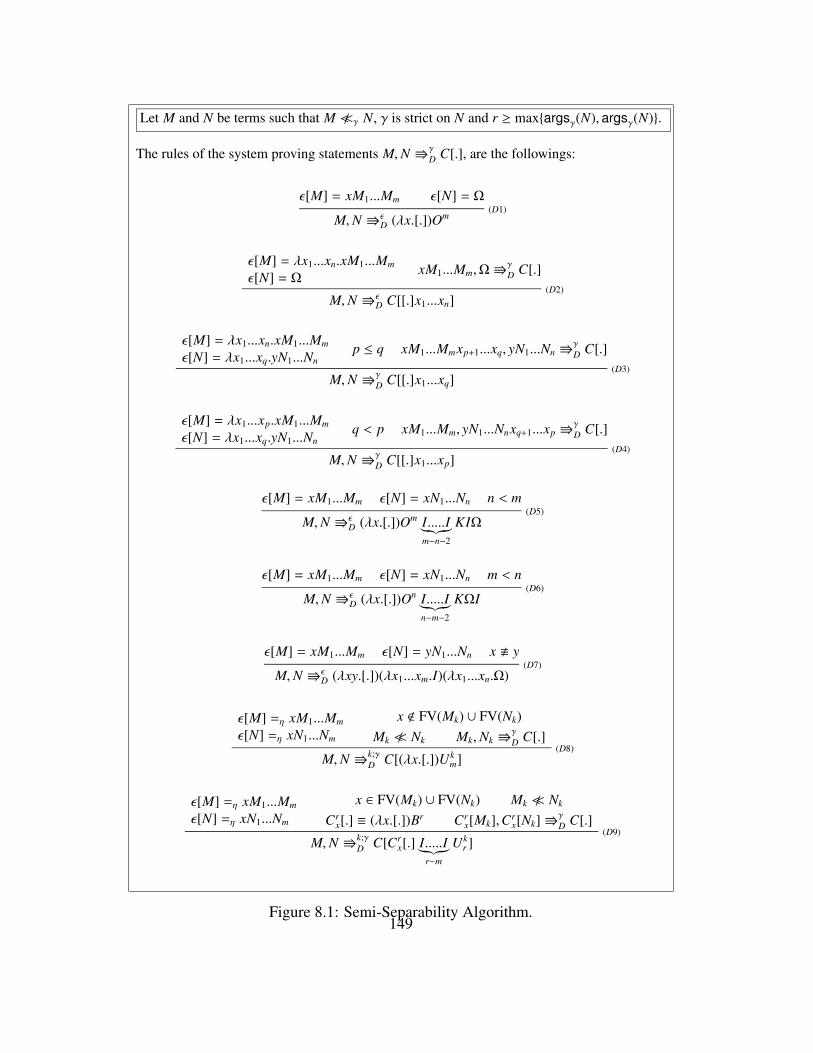
Let M and N be terms such that M 3γ N, γ is strict on N and r ≥ maxargsγ(N), argsγ(N).

The rules of the system proving statements M,N VγD C[.], are the followings:

ε[M] = xM1...Mm ε[N] = Ω(D1)

M,N VεD (λx.[.])Om

ε[M] = λx1...xn.xM1...Mm

ε[N] = ΩxM1...Mm,ΩV

γD C[.]

(D2)M,N Vε

D C[[.]x1...xn]

ε[M] = λx1...xn.xM1...Mm

ε[N] = λx1...xq.yN1...Nnp ≤ q xM1...Mmxp+1...xq, yN1...Nn V

γD C[.]

(D3)M,N Vγ

D C[[.]x1...xq]

ε[M] = λx1...xp.xM1...Mm

ε[N] = λx1...xq.yN1...Nnq < p xM1...Mm, yN1...Nnxq+1...xp V

γD C[.]

(D4)M,N Vγ

D C[[.]x1...xp]

ε[M] = xM1...Mm ε[N] = xN1...Nn n < m(D5)

M,N VεD (λx.[.])Om I.....I︸︷︷︸

m−n−2

KIΩ

ε[M] = xM1...Mm ε[N] = xN1...Nn m < n(D6)

M,N VεD (λx.[.])On I.....I︸︷︷︸

n−m−2

KΩI

ε[M] = xM1...Mm ε[N] = yN1...Nn x . y(D7)

M,N VεD (λxy.[.])(λx1...xm.I)(λx1...xn.Ω)

ε[M] =η xM1...Mm

ε[N] =η xN1...Nm

x < FV(Mk) ∪ FV(Nk)Mk 3 Nk Mk,Nk V

γD C[.]

(D8)M,N Vk;γ

D C[(λx.[.])Ukm]

ε[M] =η xM1...Mm

ε[N] =η xN1...Nm

x ∈ FV(Mk) ∪ FV(Nk) Mk 3 Nk

Crx[.] ≡ (λx.[.])Br Cr

x[Mk],Crx[Nk]V

γD C[.]

(D9)M,N Vk;γ

D C[Crx[.] I.....I︸︷︷︸

r−m

Ukr ]

Figure 8.1: Semi-Separability Algorithm.149

Proof. By induction on the derivation of M,N VγΛ

C[.].

(D1),(D2) Obvious.

(D3),(D4),(D5),(D6),(D7),(D8) By using the Confluence Theorem, they are respectively simi-lar to case (Λ1), (Λ2), (Λ3), (Λ4), (Λ5) and (Λ6) in the proof of correctness of the Λ-Separability algorithm (see Theorem 2.1.19).

(D9) The proof is similar to the proof of rule (Λ7) of the proof of correctness of the Λ-Separabilityalgorithm, using Lemma 8.6.15 instead of Lemma 2.1.16.

Proof of the Semi-separability Theorem

By Lemmas 8.6.16 and 8.6.17.

150

Part III

A Typed calculus

151

III. Introduction

PCF is a paradigmatic example of a typed functional programming language, it is based on theLCF language introduced by Scott as “logical calculus” or “algebra” for the purpose of studyingcomputability and logical properties of programs by using type theory [95].

In this part, we present a version of PCF (similar to that presented in [17]) being a typed λ-calculus with integers, successor, predecessor, conditional and recursion operators. PCF hasbecome the most popular paradigmatic language studied in semantics of programming languages,in fact many kind of semantics as been studied for it (see [1, 4, 15, 16, 72, 84, 54]).

Milner in “Fully abstract models of typed λ-calculi” [68] has introduced the key notion of full-abstraction. Two programs are said observational equivalent with respect to some operationalsematics, whenever they are interchangeable without affecting the observable outcome of thecomputation. In contrast, according to a denotational semantics the meaning of a program isits denotation; hence, two programs are denotationally equivalent if they have the same deno-tation in the model. If the denotational equivalence implies the operational equivalence, thenthe denotational semantics is said correct. If the reverse implication holds then the denotationalsemantics is said complete. If the equivalences coincide then the denotational semantics is saidfully abstract.

Plotkin in “LCF considered as a programming language” [84] and Sazonov in “Expressibilityof functions in D. Scott’s LCF language” [91] have showed that the standard interpretation ofPCF on Scott-Continous Domains is not fully abstract. In particular, the parallel-or is a con-tinuous function and it makes different the interpretation of some PCF -programs that cannot bedistinguished observationally. Moreover Plotkin by extending the syntax of PCF by a parallel-ifoperator, has obtained a programming language fully abstract with respect to Scott-ContinuousDomains (via the standard interpretation too). It is possible to show that the parallel-if and thewell-known parallel-or are interdefinables [101]. Curien in [21] showed that simply adding theparallel-or to PCF is enough to obtain the full-abstraction.

The problem of giving a semantical description of a fully abstract model of unextended PCFhas been resolved in many way [1, 68, 70, 54], moreover many efforts has been done in orderto construct spaces of “sequentials” functions corresponding to those definable in PCF withoutparallelism, as “stable functions”, “bistable functions”, “strongly stable functions”, “sequentialalgorithms”, and “manifestly sequential functions” [9, 10, 15, 16, 17, 21].

In particular, Gustave Berry has discovered stability in his study of sequential computation [9,10]. Its stable functions give a more refined denotational characterization of PCF programs thanthat of Scott Continuous Functions. Stable functions take into account the minimum amount ofinput information producing some amount of output information. Berry’s dI-domains, are Scott-domains satisfying two additional axioms, such that the ordering on functions spaces is not thepointwise ordering, but a new ordering, called the stable ordering. However, it is well-known

152

that there is some kind of stable “parallel function”, as the Gustave function.

The theory of stable functions has been rediscovered by Girard [35] as a semantic counterpart ofhis theory of dilators. Girard has introduced the category of Coherent Spaces [36], being a verynice mathematical setting where morphisms are stable functions between coherent spaces.

Many people have studied how extend a language in order to obtain the full-abstraction withrespect to some models [84, 17, 12, 72]. The general benefits of structured approaches to opera-tional semantics and connection to full abstraction are discussed in [66].

It has been observed in [55] that, already in finite dI-domains, there are stable functions thatare not Scott-continuous. We rediscovered independently the same kind of functions in coherentspaces. Namely, there are functions able to distinguish a constant function (defined on the bottomof the domain) from non-constant function.

We have showed how those functions can be added to PCF by a new control operator, namedtest?, by describing, its behavior in an operational way. Let ⇓e be our evaluation relation, let Mbe a closed term of type ι ι (namely M applied to a numeral gives back a numeral or diverges)and let Ωι be a diverging term. Morally test? can be described with the two following rules:

1. if M0 ⇓e and MΩι ⇑e then test?M ⇓e 0;

2. if M0 ⇓e and MΩι ⇓e then test?M ⇓e 1.

Nevertheless, a more constructive operational description (based on an abstract machine) will begiven in details.

This kind of operator seems correspond to a weak version of “tests” that can be done in the lan-guage SPCF (essentially a PCF endowed with some kind of errors and error-catching) definedfrom Cartwright, Curien and Felleisen in “Fully Abstract Semantics for observably sequentiallanguages” [17]. The control test considered together with a Gustave-like operator have beenjoined to the syntax of PCF , by obtaining a new language StPCF endowed with an operationalsemantics.

Hence we have showed that coherent spaces give a fully abstract model for PCF extended bytest? and a Gustave-Operator (we called it, StPCF ), via the standard interpretation. In par-ticular, we show that all finite cliques of coherent spaces being interpretation of a PCF -StPCFtype are represented by a StPCF -program.

After we have developped the results of this part of the thesis, we have discovered that the sameproblem was considered first by Jim and Meyer in “Full Abstraction and Context Lemma” [55],by considering dI-domains. They have showed some negative results. First they define in adenotational way, the True-Separator function (that actually correspond to a boolean version ofour operator test?), hence they show that this operator break-down the coincidence between theapplicative-preorder on terms and the contextual-preorder. Finally, they show that with their huge

153

class of “linear ground operational rules” defining some PCF -like rules of evaluation the beforecoincidence cannot be break-down. Since the True-Separator function is both stable and stronglystable, they conclude that it is hard to find an extension of PCF with operators endowed with anoperational desciption being fully abstract with respect to stable and strongly stable function.

Indeed, our operational decription of the operator test? fall down from their PCF -like rules.So the results presented in [55] can be reread as:

it is not possible to find a conservative extension of PCF fully abstract with respectto stable functions (and strongly stable functions) without an operator as test?,moreover the operational description of test? cannot be defined by using theirPCF -like rules.

The relations between StPCF and strongly stable functions are unexplored, although we areinterested in.

154

Chapter 9

Stable PCF

PCF [84, 68] is an essential programming language based on Scott’s LCF logic of computablefunctions [46]. It can be extended in order to give out a new language fully abstract with respectto the coherent spaces of Girard [35, 36], as we will in this chapter.

9.1 Syntax of PCFWe present a version of PCF (similar to that presented in [17]) being a typed λ-calculus withintegers, successor, predecessor, conditional and recursion operators.

Definition 9.1.1 (Types) Let ι be a type constant or ground.The types of PCF are generated by the following grammar:

σ ::= ι | (σ τ)

where σ, τ, ... are metavariables ranging over types of PCF .

As customary the associates to right, thus σ1 σ2 σ3 is an abbreviation for σ1 (σ2 σ3). Furthermore, it is easy to see that all types τ have the shape τ1 ... τn ι, forsome type τ1, ..., τn (n ∈ ).

Definition 9.1.2 The level of a type is defined inductively as follows

• level(ι) = 0

• level(σ τ) = 1 + maxlevel(σ), level(τ).

155

Let Var be a numerable set of variables.

Definition 9.1.3 (PCF -words)The words of PCF are defined by the following grammar:

M ::= x | (λxσ.N) | (PQ) | Yσ

| if0 | succ | pred | n

where x ∈ Var and σ is a type, while M, N, P, Q, ... are metavariables ranging over the wordsof PCF and n, m, ... are metavariables ranging over numerals, namely the numerable constants0, 1, 2, ......

The λ-abstraction is the only binder as customary in λ-calculi, while Yσ is the recursion operatorof type (σ σ) σ for each type σ, if0 is a conditional operator having type ι ι ιι, numerals represent natural numbers and have type ι, while succ and pred are successorand predecessor operator having type ι ι.

As customary, MNP will be used as an abbreviation for (MN)P, while λxσyτ.P is an abbreviationfor (λxσ.(λyτ.P)).

Note that variables are untyped, but the λ-abstraction add some type information to the variable.The language of PCF will be a subset of the PCF -words.

Definition 9.1.4The set of free variables of a word M is denoted FV(M) and it is defined as follows:

FV(x) = x FV(n) = ∅ FV(if0 ) = ∅FV(MN) = FV(M) ∪ FV(N) FV(succ ) = ∅ FV(Yσ) = ∅FV(λxσ.N) = FV(N) \ x FV(pred ) = ∅

M is closed if and only if FV(M) = ∅, otherwise M is said open. A variable x occurring in a termM is said bound if and only if x < FV(M).

Words are considered up to α-equivalence, namely a bound variable can be renamed provided nofree variable be captured; so, λxσ.x =α λy

σ.y while λxσ.xy ,α λyσ.yy .

As customary, M[N/x] denotes the capture-free substitution of all free occurrences of x in M by N.

Not all words are well-typed, the “typing system” establishing valid typed terms and their typesfollows.

156

Definition 9.1.5 (PCF -language) A basis B is a finite list of pairs variable-type of the shape

x1 : σ1, ....., xn : σn (n ∈ )

such that xi = x j implies i = j (1 ≤ i, j ≤ n), i.e. there is not variable repetition.A term of the PCF -language is a word M being in the conclusion B ` M : σ of a derivation builtby using the following rules:

B, x : σ, B′ ` x : σ B ` n : ι B ` Yσ : (σ σ) σ

B ` P : σ τ B ` Q : σ

B ` PQ : τ

B, x : σ, B′ ` N : τ

B, B′ ` λxσ.N : σ τ

B ` succ : ι ι B ` pred : ι ι B ` if0 : ι ι ι ι

B ` M : σ is a typing judgment or simply typing if and only if, it is the conclusion of a derivation,before defined; moreover, M is said the subject of the typing.A program is a closed term of type ι.

As customary we will write B ` M : σ when the typing is a conclusion of a derivation built byusing the previous rules, while we will write B 0 M : σ when a such derivation does not exist. Ifthe basis of a typing is empty then we will write simply ` M : σ.

Note that B ` λxν.M : σ implies that there is a type τ such that σ ≡ ν τ.

For sake of simplicity, in the follows only words being terms will be considered, although some-times its typings will be omitted.

Definition 9.1.6 (PCF -contexts) Let C[.] be a word generated by the following grammar:

C[.] ::= x | [.] | λxσ.C[.] | (C[.]D[.]) | Yσ

| if0 | succ | pred | n

where [.] is a new symbol (said hole), x ∈ Var and σ is a type, while C[.],D[.], ... will be used inthe follows as metavariables ranging over contexts and n, m, ... are metavariables ranging overnumerals.

Informally, a context forσ is a term with one or more “holes” [.] in them, where [.] is an holdplacefor an unknown term of type σ.

157

Let C[.] be a context; as customary, by replacing all occurrences of holes of C[.] by a term M anew term P ≡ C[M] is obtained where the free variables of M can be captured by λ-abstractionsof C[.].

A calculus based on some reduction rules can be defined in a similar way to that used for theλ-calculus, as in [72]; however, we are interested only in the leftmost reduction strategy, so weallow only lazy reductions i.e. reduction not under the scope of a λ-abstraction.

Definition 9.1.7 Let→e be the reduction for PCF defined by the following rules:

(λxσ.M)N→e M[N/x]M→e M

′

MN→e M′N

YσM→e M(YσM)

if0 0 M N→e M if0 n + 1 M N→e N

succ n→e n + 1 pred n + 1→e n

N→e N′

MN→e MN′ (if M is succ , pred or if0 ).

where n is a numerals and the meaning of n + 1 is straightforward.

Note that→e is lazy in the sense that, it cannot be applied under abstractions.

The reduction→e is confluent, i.e. it enjoy the Church-Rosser property. Furthermore, it make usable to define an operational semantics by a partial function Exec from programs to numerals.

Exec(M) = n if and only if M→∗e n, for a program M and a numeral n;

where→∗e is the transitive reflexive closure of→e.

Definition 9.1.8 (Subject Reduction) If B ` M : σ and M→e N then B ` N : σ too.

Proof. Easy.

Clearly Exec induces a lazy call-by-name deterministic well-defined evaluation, that can be for-malized in a SOS-style in a straightforward manner.

158

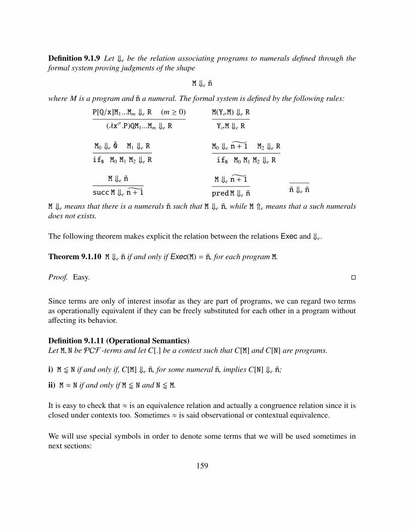
Definition 9.1.9 Let ⇓e be the relation associating programs to numerals defined through theformal system proving judgments of the shape

M ⇓e n

where M is a program and n a numeral. The formal system is defined by the following rules:

P[Q/x]M1...Mm ⇓e R (m ≥ 0)

(λxσ.P)QM1...Mm ⇓e R

M(YσM) ⇓e R

YσM ⇓e R

M0 ⇓e 0 M1 ⇓e R

if0 M0 M1 M2 ⇓e R

M0 ⇓e n + 1 M2 ⇓e R

if0 M0 M1 M2 ⇓e R

M ⇓e n

succ M ⇓e n + 1

M ⇓e n + 1

pred M ⇓e nn ⇓e n

M ⇓e means that there is a numerals n such that M ⇓e n, while M ⇑e means that a such numeralsdoes not exists.

The following theorem makes explicit the relation between the relations Exec and ⇓e.

Theorem 9.1.10 M ⇓e n if and only if Exec(M) = n, for each program M.

Proof. Easy.

Since terms are only of interest insofar as they are part of programs, we can regard two termsas operationally equivalent if they can be freely substituted for each other in a program withoutaffecting its behavior.

Definition 9.1.11 (Operational Semantics)Let M, N be PCF -terms and let C[.] be a context such that C[M] and C[N] are programs.

i) M / N if and only if, C[M] ⇓e n, for some numeral n, implies C[N] ⇓e n;

ii) M ≈ N if and only if M / N and N / M.

It is easy to check that ≈ is an equivalence relation and actually a congruence relation since it isclosed under contexts too. Sometimes ≈ is said observational or contextual equivalence.

We will use special symbols in order to denote some terms that we will be used sometimes innext sections:

159

• Ωσ will be used in order to denote the term defined by induction σ as follows:

Ωι ≡ Yι(λxι.x) Ωµτ ≡ λxµ.Ωτ.

• by using Ωσ, it is possible to define terms Ynσ (n ∈ ) in the following way:

– Y0σ ≡ Ω(σσ)σ

– Yn+1σ ≡ λxσσ.x(Yn

σ x).

Let M be a program; as a notational convention we will write simply M ⇓e whenever M ⇓e n, forsome n. Furthermore, we will write M ⇑e if there are no derivation proving M ⇓e n.

Lemma 9.1.12 i) If ΩσM0...Mm (m ∈ ) is a program then ΩσM0...Mm ⇑e.

ii) Let YσM0...Mm (m ∈ ) be a program.YσM0...Mm ⇓e n if and only if Yk

σM0...Mm ⇓e n, for some k ∈ .

Proof.

i) Easy.

ii) (⇒) YσM0...Mm ⇓e n implies that M0(YσM0)...Mm ⇓e n too; by induction on the latter derivationit is possible to show that M0(M0.....(ΩσM0)...)︸ ︷︷ ︸

k

M1...Mm ⇓e n, for some k ∈ . The proof follows

by definition of Ykσ.

(⇐) M0(M0.....(ΩσM0)...)︸ ︷︷ ︸k

M1...Mm ⇓e n for some k ∈ implies that YσM0...Mm ⇓e n by induction

on the derivation.

In literature PCF is often presented with booleans and some operator on they. We consideredonly integers (as done in [17]), since the differences between the two formalizations are mean-ingless for our purposes.

However, sometimes in the follows some simple example will be showed by using booleans; thuswe formalize an extension of PCF .

Definition 9.1.13 (PCF+++B-language)

• Types of PCF+++B are the types of PCF extended with the ground type o .

160

• The words of PCF+++B are the words generated by the grammar of PCF extended withtt | ff | zero? | cond .

• The terms of PCF+++B are defined as that of PCF , by adding the following rules for typing:

B ` tt : o B ` ff : o

B ` zero? : ι o B ` cond : o ι ι ι

Clearly FV(tt) = FV(ff) = FV(zero?) = FV(cond) = ∅.In order to formalize the behavior of tt, ff, zero?, cond, the reduction rule→e can be extendedby:

cond tt M N→e M cond ff M N→e N

zero? 0→e tt zero? n + 1→e ff

N→e N′

MN→e MN′ (if M is zero? or cond).

The behavior of tt, ff, zero?, cond can be described in a SOS-style by extending the formalsystem for the relation ⇓e with the rules:

M0 ⇓e tt M1 ⇓e R

cond M0 M1 M2 ⇓e R

M0 ⇓e ff M2 ⇓e R

cond M0 M1 M2 ⇓e R

M ⇓e 0

zero?M ⇓e tt

M ⇓e n + 1

zero?M ⇓e ff

Let M,N be two PCF -programs, namely closed terms of type ι. It is easy to see that they areoperationally equivalent in PCF+++B if and only if they are operationally equivalent in PCF .

9.2 Mathematical Preliminaries

The standard mathematical notation and terminology will be used for sets and functions, howeversome definition will be recalled.

If X is a finite set then ‖X‖ is the number of elements of X.

161

Definition 9.2.1 A partial order or poset is a pair (D,v) where D is a set and v is an orderrelation, namely a binary relation such that, for each x, y, z ∈ D:

• x v x (reflexive);

• if x v y and y v x then x = y (antisymmetric);

• if x v y and y v z then x v z (transitive).

By abusing the notation often the poset will be simply denoted by D.

A subset X ⊆ D is bounded if and only if it has an upper bound; sometimes x, y ∈ D are saidconsistent when there is z ∈ D such that x, y v z. A poset D is said consistently complete if andonly if there is the least upper bound of each pair of consistent element of D.

An element of D is said bottom and denoted⊥⊥⊥⊥⊥⊥⊥⊥⊥ if and only if⊥⊥⊥⊥⊥⊥⊥⊥⊥ v d, for each d ∈ X.

A least upper bound or supremum or join of X ⊆ D is an element d of D such that x v d, foreach x ∈ X. It is easy to check that the supremum of a set is unique, if it exists.

A partial order D is flat when, for all x, y ∈ D, if x v z then x =⊥⊥⊥⊥⊥⊥⊥⊥⊥ or x = z.

A subset X of D is directed if ∀x, x′ ∈ X ∃x′′ ∈ X such that x ≤ x′′ and x′ ≤ x′′, namely for eachpair of elements of X there is an upper bound in X.

Definition 9.2.2 A cpo is a poset D with bottom⊥⊥⊥⊥⊥⊥⊥⊥⊥ ∈ D such that if X ⊆ D is directed then thereis tX ∈ D being the least upper bound of X.

Let A, B be cpos; a function f : A → B is monotonic if and only if ∀x, x′ ∈ A x ≤A x′ thenf (x) ≤B f (x′).

A function f : A→ B is Scott-continuous [92, 93] if and only if it preserves limit of directed set,namely if X ⊆ D is directed then

f (tX) = t f (X)

Definition 9.2.3 A category C is a 4-tuple (Ob jC, homC, , idC) where

1. Ob jC is a collection of objects;

2. homC(A, B) is a collection of arrows, for all A, B ∈ Ob jC;

3. is a partial composition operation on arrows such that:

162

• if f ∈ homC(A, B) and g ∈ homC(B,C) then g f ∈ homC(A,C);

• ( f g) h = f (g h) when the composition is defined.

4. idC is a total function associating to each A ∈ Ob jC an arrow idAC ∈ homC(A, A) such that:

idAC f = f idA

C = f

for all f ∈ homC(A, A).

Let f ∈ homC(A, B); f is an iso if and only if there exists f −1 ∈ homC(B, A) such that f f −1 = idAC

and f −1 f = idBC.

An object 1 in a category C is said terminal if and only if there exists exactly one arrow inhomC(A, 1), for each A ∈ Ob jC.

Definition 9.2.4 Let A0, A1 ∈ Ob jC; an object P of the category with two arrows πi ∈ homC(P, Ai)(i ≤ 1) is said categorical product if and only if, for each B ∈ Ob jC and each fi ∈ homC(B, Ai)(i ≤ 1), there exists a unique arrow 〈 f0, f1〉 ∈ homC(B, P) such that

πi 〈 f0, f1〉 = fi i ≤ 1

〈π0 f , π1 f 〉 = f

for each f ∈ homC(B, P).

As customary a product for A0, A1 will be denoted simply A0 × A1. Sometimes × will be usedin order to denote the set-theoretical cartesian product, however a different notation will be usedfor the categorical products of the categories considered in the follow.

Definition 9.2.5 A category C is said cartesian if and only if it has at least a terminal object anda there is a categorical product for any two objects of C.

The exponent of two objects is the next key notion.

Definition 9.2.6 Let A, B ∈ Ob jC; an exponent for A, B is an object BA with an arrow eval ∈homC(BA × A, B) such that, for each C ∈ Ob jC, for each f ∈ homC(C × A, B) there is a uniqueh ∈ homC(C, BA) satisfying

eval (h × idA) = f

where f × g = 〈 f π1, g π2〉.

163

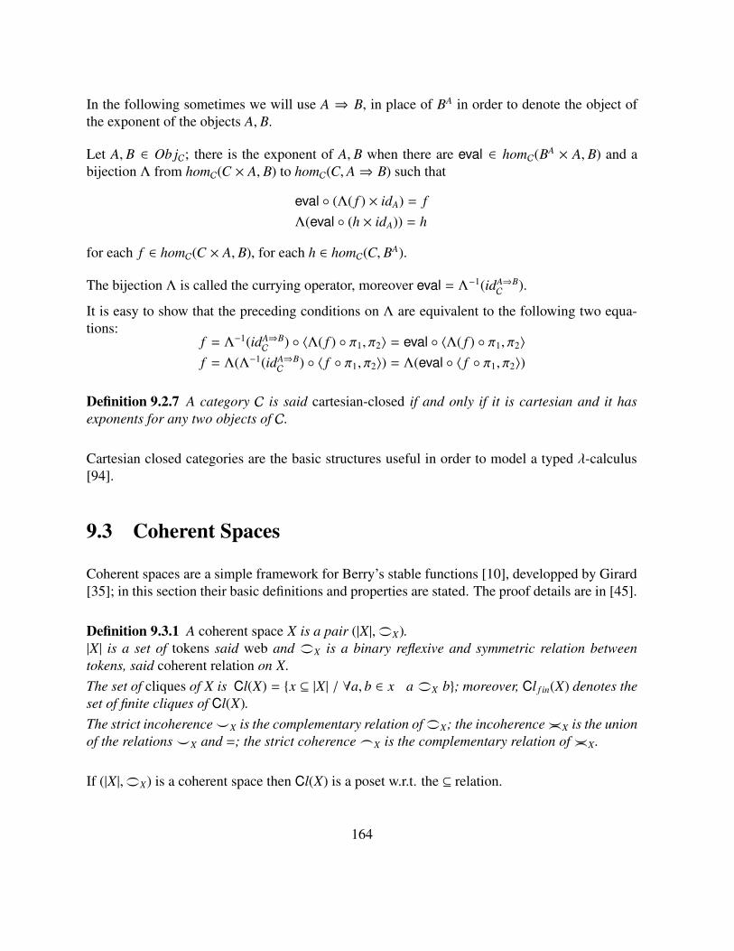
In the following sometimes we will use A ⇒ B, in place of BA in order to denote the object ofthe exponent of the objects A, B.

Let A, B ∈ Ob jC; there is the exponent of A, B when there are eval ∈ homC(BA × A, B) and abijection Λ from homC(C × A, B) to homC(C, A⇒ B) such that

eval (Λ( f ) × idA) = fΛ(eval (h × idA)) = h

for each f ∈ homC(C × A, B), for each h ∈ homC(C, BA).

The bijection Λ is called the currying operator, moreover eval = Λ−1(idA⇒BC ).

It is easy to show that the preceding conditions on Λ are equivalent to the following two equa-tions:

f = Λ−1(idA⇒BC ) 〈Λ( f ) π1, π2〉 = eval 〈Λ( f ) π1, π2〉

f = Λ(Λ−1(idA⇒BC ) 〈 f π1, π2〉) = Λ(eval 〈 f π1, π2〉)

Definition 9.2.7 A category C is said cartesian-closed if and only if it is cartesian and it hasexponents for any two objects of C.

Cartesian closed categories are the basic structures useful in order to model a typed λ-calculus[94].

9.3 Coherent Spaces

Coherent spaces are a simple framework for Berry’s stable functions [10], developped by Girard[35]; in this section their basic definitions and properties are stated. The proof details are in [45].

Definition 9.3.1 A coherent space X is a pair (|X|, _X).|X| is a set of tokens said web and _X is a binary reflexive and symmetric relation betweentokens, said coherent relation on X.The set of cliques of X is Cl(X) = x ⊆ |X| / ∀a, b ∈ x a _X b; moreover, Cl f in(X) denotes theset of finite cliques of Cl(X).The strict incoherence_X is the complementary relation of _X; the incoherence _X is the unionof the relations _X and =; the strict coherence ^X is the complementary relation of _X.

If (|X|, _X) is a coherent space then Cl(X) is a poset w.r.t. the ⊆ relation.

164

Let X be a coherent space; tokens will be basic bits of information. Further two different tokensa, b will be coherent if and only if its information is “compatible”, namely if it makes sense tojoin they in a more complex information. As example, tokens of a function from N to N, will besomething like a ≡ (0 7→ 3), b ≡ (1 7→ 3) and c ≡ (0 7→ 5) and so on; the obvious coherencerelations will be a ^ b, b ^ c, but a _ c in fact there are no functions in N −→ N that can giveback on the input 0 both the outputs 3 and 5.

Lemma 9.3.2 Let X be a coherent space.

i) ∅ ∈ Cl(X).

ii) a ∈ Cl(X), for each a ∈ |X|.iii) If y ⊆ x and x ∈ Cl(X) then y ∈ Cl(X).

iv) If D ⊆ Cl(X) is directed then ∪D ∈ Cl(X).

Proof. Easy.

Hence, the cliques of a coherent space with the set-inclusion form a cpo.Let x, x′ be sets; x ⊆ f in x′ means that x ⊆ x′ and x is finite.

Definition 9.3.3Let X and Y be coherent spaces and f : Cl(X) −→ Cl(Y) be a monotonic function.

• f is said continuous if and only if ∀x ∈ Cl(X) ∀b ∈ f (x) implies that ∃x0 ⊆ f in x such thatb ∈ f (x0).

• f is said stable if and only if ∀x ∈ Cl(X) ∀b ∈ f (x) implies that ∃x0 ⊆ f in x such thatb ∈ f (x0) and, ∀x′ ⊆ x if b ∈ f (x′) then x0 ⊆ x′.

The continuity ask for the existence of a finite part of the input for which every token in output isproduced, while the stability ask for a minimum finite part of the input for which an output tokenis produced.

Equivalent formulations of continuity and stability are formalized in what follows.

Lemma 9.3.4

165

i) Let X and Y be coherent spaces and f : Cl(X) −→ Cl(Y) be a monotonic function.f is continuous if and only if f (∪D) = ∪ f (x)/x ∈ D, for each D ⊆ Cl(X) directed.

ii) Let X and Y be coherent spaces and f : Cl(X) −→ Cl(Y) be a continuous function.f is stable if and only if ∀x, x′ ∈ Cl(X), x ∪ x′ ∈ Cl(X) implies f (x ∩ x′) = f (x) ∩ f (x′).

It is easy to check that coherent spaces and stable morphisms form a category denoted by .

Definition 9.3.5 Let X1 and X2 be coherent spaces.X1&X2 is the coherent space having |X&Y | = (1×|X1|)∪(2×|X2|) as web; while, ∀(i, a), ( j, b) ∈|X1&X2| (i, a) _X1&X2 ( j, b) if and only if i , j or, i = j and a _Xi b.

It is easy to check that X1&X2 is a categorical product in for the spaces X1, X2. Since1 = (∅, ∅) is terminal object for , it follows that is cartesian.

Stable functions can be represented as cliques in some coherent space.

Definition 9.3.6 Let X and Y be coherent spaces.The trace tr( f ) of the stable function f : Cl(X) −→ Cl(Y) is the set of pair (x0, b) ∈ Cl f in(X) × |Y |such that b ∈ f (x0) and ∀x ⊆ x0, b ∈ f (x) implies x = x0.

A coherent space having traces of functions as clique is expected.

Definition 9.3.7 Let X and Y be coherent spaces.X ⇒ Y is the coherent space having |X ⇒ Y | = Cl f in(X) × |Y | as web, while if (x0, b0), (x1, b1) ∈|X ⇒ Y |, then (x0, b0) _X⇒Y (x1, b1) under the following conditions:

i) x0 ∪ x1 ∈ Cl(X) implies b0 _Y b1;

ii) x0 ∪ x1 ∈ Cl(X) and b0 = b1 imply x0 = x1.

The bridge between stable functions and clique of corresponding coherent space X ⇒ Y is givenin the next lemma.

Lemma 9.3.8 If f : Cl(X) −→ Cl(Y) is a stable function then tr( f ) ∈ Cl(X ⇒ Y).

Let X,Y be coherent spaces and t ∈ Cl(X ⇒ Y); F (t) : Cl(X) −→ Cl(Y) will be a function suchthat ∀x ∈ Cl(X), F (t)(x) = b ∈ |Y | / ∃x0 ∈ Cl(X) (x0, b) ∈ t ∧ x0 ⊆ x.

166

Lemma 9.3.9 Let X,Y be coherent spaces and t ∈ Cl(X ⇒ Y).F (t) : Cl(X)→ Cl(Y) is a stable function.

It is easy to check that is a cartesian closed category, by defining the arrow eval ∈ homC(BA×A, B) of the Definition 9.2.6 as

eval(z) = b ∈ B | ∃(1, (x0, b)) ∈ z such that ∀a ∈ x0 (2, a) ∈ z.

9.4 Interpretation of PCFPlotkin [84] as showed how it is possible to interpret the PCF syntax on Scott Domains by a settheoretical interpretation based on a standard interpretation carrying out some natural constrainton models of PCF .

Although the same constraints can be formalized in a categorical style, for sake of simplicity, weprefer to give a set theoretical interpretation in order to avoid the need of some cumbersome (forour purposes) formalization of the “stable” order on arrows.

In fact, in order to give a categorical interpretation for Yσ usually a cpo-enriched category isdefined by making explicit an order between arrows, but unfortunately stable morphisms are notordered in an extensional way [17, 4].

Definition 9.4.1The interpretation is standard when ground types are interpreted on flat partial orders.

We will give a standard interpretation of PCF as a mapping from the syntax to the coherentspaces category, namely types will be mapped in objects (coherent spaces) and terms on cliques.

Definition 9.4.2

i) Let B denote the coherent space of boolean values, namely (T,F), _B) such that T _B F;thus Cl(B) = ∅, T, F.

T F

∅

167

ii) Let N denote the coherent space of natural numbers, namely (|N|, _N) such that |N| = and

m ^N n if and only if m = n, for all m, n ∈ |N|.Thus Cl(N) = ∅ ∪ n / n ∈ |N| .

0 1 n

∅

Note Cl(B) and Cl(N) endowed with the set theoretical inclusion forms flat partial orders.As customary emphatic brackets will be used as notation in order to formalize both the correspon-dence between types and coherent spaces and the correspondence between terms and cliques.

The standard interpretation of PCF put ~ι = N, while ~σ τ = ~σ⇒ ~τ. The interpreta-tion can be extended to PCF+++B by putting ~o = B.

In order to give an interpretation to a PCF -term M we need to know its typing, actually theinterpretation will interpret typing i.e. terms with type (although implicitly).Let B be a basis, so EnvB will be a set of function mapping a variable x in a clique of ~σ whenx : σ ∈ B. If ρ ∈ EnvB, x : σ ∈ B and x ∈ ~σ then ρ[x/x] ∈ EnvB is the environment such that

ρ[x/x](y) =

x if x ≡ y

ρ(y) otherwise.

Definition 9.4.3 Let B ` M : σ be a typing of PCF and let ρ ∈ EnvB.The interpretation of M with respect to ρ is denoted ~Mρ and it is a clique of ~σ obtained in thefollowing way, by induction on M.

• ~xρ = ρ(x).

• ~λxµ.Pρ =

(x0, b) ∈ Cl(~µ) × |~τ|

∣∣∣∣∣∣b ∈ ~Pρ[x0/x] and∀y ⊆ x0 b ∈ ~Pρ[y/x] implies y = x0

where σ ≡ µ τ, for some types µ, τ.

• ~PQρ = F (~Pρ)~Qρ where F is the operator defined just before the Definition 9.3.9.

• Let σ ≡ (τ τ) τ and x ∈ Cl f in(~τ τ); we will write (z0, b0) Ex (z1, b1) if andonly if either (z0, b0) = (z1, b1), or b0 ∈ z1, or there is (z2, b2) ∈ x such that b2 ∈ z1 and(z0, b0) Ex (z2, b2), for all (z0, b0), (z1, b1) ∈ x.

168

~Yτ =

(x, a)

∣∣∣∣∣∣∣∣∣∣∣∣∣

(x, a) ∈ Cl f in(~τ τ) × |~τ| ;(x,Ex) is a finite partial order;there is a unique (z, b) ∈ x being the top such that b = a;if (z, c) ∈ x and d ∈ z then ∃(y, e) ∈ x such that e = d.

• ~if0 = (0, (n, (∅, n))) / n ∈ ∪ (m, (∅, (n, n))) / n ∈ and m , 0 .• ~nρ = n, for each n ∈ .

Except for Yτ, it is easy to check that the interpretation function is well defined.

Note that, if (x0, a) ∈ ~Yτ then (x,Ex) has at least minimal element of the shape (∅, b); moreover,(z, b) ∈ x0 is minimal if and only if z = ∅. Let us remark that (x0, a) is a partial order (not simplya preorder), so there is no “loop” in the structure.

Let (x0, a) ∈ ~Yτ and (z, b) ∈ x0; if x0 (z,b)= (z′, b′) ∈ x0 | (z′, b′) Ex0 (z, b) then, it is easy tosee that (x0 (z,b), b) ∈ ~Yτ.

Lemma 9.4.4 If (x0, a0), (x1, a1) ∈ ~Yτ then (x0, a0) _~(ττ)τ (x1, a1).

Proof. Note that ‖x0∪ x1‖ = 0 is not possible, since xk , ∅ (k ≤ 1) by definition of interpretationof Yτ. The conditions of coherence are proved, by contraposition.

1. We will prove that a0 _~τ a1 implies x0 ∪ x1 < Cl(~τ τ), by induction on ‖x0 ∪ x1‖.‖x0 ∪ x1‖ = 1 would imply x0 = (∅, a0) = (∅, a1) = x1, so the case is not possible.Let ‖x0∪ x1‖ = 2. The case x0 = (∅, b), (b, a0) = x1 is not possible. Hence x0 = (∅, a0),x1 = (∅, a1) and the proof is immediate, since a0 _~τ a1 implies (∅, a0) _~ττ (∅, a1),thus (∅, a0), (∅, a1) < Cl(~τ τ).Let ‖x0∪x1‖ ≥ 3; by definition of interpretation of Yτ there are (z0, a0) ∈ x0 and (z1, a1) ∈ x1.If z0 ∪ z1 ∈ Cl(~τ) then (z0, a0) _~ττ (z1, a1), since by hypothesis a0 _~τ a1, hencex0 ∪ x1 < Cl(~τ τ).Let z0 ∪ z1 < Cl(~τ), so there are b0 ∈ z0, b1 ∈ z1 such that b0 _~τ b1, moreoverthere are (z0

0, b0) ∈ x0 and (z11, b1) ∈ x1 such that (x0 (z0

0,b0), b0), (x1 (z11,b1), b1) ∈ ~Yτ, by

interpretation of Yτ. Nevertheless ‖x0 (z00,b0) ∪x1 (z1

1,b1) ‖ < ‖x0 ∪ x1‖, so by inductivehypothesis x0 (z0

0,b0) ∪x1 (z11,b1)< Cl(~τ τ).

Since xk (zkk ,bk)⊆ xk (k ≤ 1), the proof is done.

2. We will prove that x0 , x1 and a0 = a1 then x0 ∪ x1 < Cl(~τ τ), by induction on‖x0 ∪ x1‖.‖x0 ∪ x1‖ = 1 is not possible, as in the previous case. ‖x0 ∪ x1‖ = 2 would imply eitherx0 = (∅, a0), (∅, a1) = x1 and a0 = a1, or x0 = (∅, b), (b, a0) = x1, so both cases are

169

not possible.Let ‖x0 ∪ x1‖ ≥ 3; by definition of interpretation of Yτ there is (z0, a0) ∈ x0 and there is(z1, a1) ∈ x1. If z0 , z1 then (z0, a0) _~ττ (z1, a0) and the proof is done, otherwise letz0 = z1. The case z0 = z1 = ∅ is against the hypothesis that ‖x0 ∪ x1‖ ≥ 3, since it wouldimply x0 = (∅, a0) = (∅, a1) = x1. Hence by definition of interpretation of Yτ, for eachb ∈ z0 = z1 there are (zb

0, b) ∈ x0, (zb1, b) ∈ x1 such that (x0 (zb

0,b), b), (x1 (zb1,b), b) ∈ ~Yτ.

If zb0 , zb

1, for some b ∈ z0, then (zb0, b) _~ττ (zb

1, b) and the proof is immediate.Otherwise, x0 , x1 implies that there is b′ ∈ z0 = z1 and there are (z′0, b

′) ∈ x0, (z′1, b′) ∈ x1

such that (x0 (z′0,b′), b′), (x1 (z′1,b′), b

′) ∈ ~Yτ and x0 (z′0,b′), x1 (z′1,b′).Nevertheless ‖x0 (z′0,b′) ∪x1 (z′1,b′) ‖ < ‖x0 ∪ x1‖, thus x0 (z′0,b′) ∪x1 (z′1,b′)< Cl(~τ τ)by induction. Since xk (z′k ,b′)⊆ xk (k ≤ 1), the proof is done.

Let x ∈ Cl f in(~τ τ); so, we can define

F n(x) =

∅ if n = 0F (x)(F n−1(x)) otherwise.

Lemma 9.4.5 F n(x) ⊆ F n+1(x).

Proof. By induction on n. If n = 0 the proof is trivial, so let n ≥ 1.

F n(x) =b | ∃(x0, b) ∈ x ∧ x0 ⊆ F n−1(x)

⊆ b | ∃(x0, b) ∈ x ∧ x0 ⊆ F n(x)

= F n+1(x)

since F n−1(x) ⊆ F n(x) by induction.

Theorem 9.4.6 i) If x ∈ Cl(~σ σ) then F (~Yσρ)(x) =⋃

n≥0

F n(x).

ii) ~Yσ =⋃

n≤0~Y(n)σ .

iii) F (~λxσ.Mρ)(x) = ~Mρ[x/xσ] where x ∈ ~σ.

iv) ~if0 ρ x y z =

y if x = 0z if x = n and n , 0

∅ otherwise.

Proof.

170

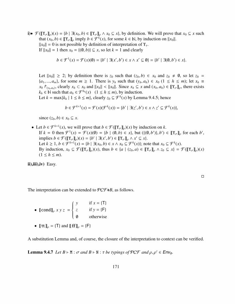
i)• F (~Yσρ)(x) = b | ∃(x0, b) ∈ ~Yσρ ∧ x0 ⊆ x, by definition. We will prove that x0 ⊆ x suchthat (x0, b) ∈ ~Yσρ imply b ∈ F k(x), for some k ∈ , by induction on ‖x0‖.‖x0‖ = 0 is not possible by definition of interpretation of Yτ.If ‖x0‖ = 1 then x0 = (∅, b) ⊆ x, so let k = 1 and clearly

b ∈ F 1(x) = F (x)(∅) = b′ | ∃(x′, b′) ∈ x ∧ x′ ⊆ ∅ = b′ | ∃(∅, b′) ∈ x.

Let ‖x0‖ ≥ 2; by definition there is z0 such that (z0, b) ∈ x0 and z0 , ∅, so let z0 =

a1, ..., am, for some m ≥ 1. There is yh such that (yh, ah) ∈ x0 (1 ≤ h ≤ m); let xh ≡x0 (yh,ah), clearly xh ⊂ x0 and ‖xh‖ < ‖x0‖. Since xh ⊆ x and (xh, ah) ∈ ~Yσρ, there existskh ∈ such that ah ∈ F kh(x) (1 ≤ h ≤ m), by induction.Let k = maxkh | 1 ≤ h ≤ m, clearly z0 ⊆ F k(x) by Lemma 9.4.5; hence

b ∈ F k+1(x) = F (x)(F k(x)) = b′ | ∃(z′, b′) ∈ x ∧ z′ ⊆ F k(x),

since (z0, b) ∈ x0 ⊆ x.

• Let b ∈ F k+1(x), we will prove that b ∈ F (~Yσρ)(x) by induction on k.If k = 0 then F 1(x) = F (x)(∅) = b | (∅, b) ∈ x, but ((∅, b′), b′) ∈ ~Yσρ for each b′,implies b ∈ F (~Yσρ)(x) = b′ | ∃(x′, b′) ∈ ~Yσρ ∧ x′ ⊆ x.Let k ≥ 1, b ∈ F k+1(x) = b | ∃(x0, b) ∈ x ∧ x0 ⊆ F k(x); note that x0 ⊆ F k(x).By induction, x0 ⊆ F (~Yσρ)(x), thus b ∈ a | (z0, a) ∈ ~Yσρ ∧ z0 ⊆ x = F (~Yσρ)(x)(1 ≤ h ≤ m).

ii),iii),iv) Easy.

The interpretation can be extended to PCF+++B, as follows.

• ~condρ x y z =

y if x = Tz if y = F∅ otherwise

• ~ttρ = T and ~ffρ = F

A substitution Lemma and, of course, the closure of the interpretation to context can be verified.

Lemma 9.4.7 Let B ` M : σ and B ` N : τ be typings of PCF and ρ, ρ′ ∈ EnvB.

171

i) If ρ(x) ⊆ ρ′(x), for all FV(M), then ~Mρ ⊆ ~Mρ′ .ii) If x : τ ∈ B then ~M[N/x]ρ = ~Mρ[ ~Nρ/x].

iii) ~Mρ = ~Nρ implies ~C[M]ρ = ~C[N]ρ, for all C[ ] respecting types.

Proof.

i) By induction on M. If M ∈ Var ∪ succ , pred , if0 , Yσ, n then the proof is immediate.If M ≡ P0P1 then the proof follow by induction, since ~Piρ ⊆ ~Piρ′ (i ∈ 0, 1). IfM ≡ (λxσ.P) the proof follows by induction again, since ~Pρ[z/x] ⊆ ~Pρ′[z/x], for eachz ∈ ~σ, since x < FV(λxσ.P).

ii) Similar to the previous case.

iii) By induction on the shape of C[.].

Furthermore,the interpretation satisfies property of adequateness.

Theorem 9.4.8 Let M, N ∈ PCF . If M→e N then ~Mρ = ~Nρ.

Proof. We check here only some cases.

• By lemma 9.4.7

~(λxσ.M)Nρ = F (~λxσ.Mρ)~Nρ =

= b | ∃x0 (x0, b) ∈ ~λxσ.Mρ ∧ x0 ⊆ ~Nρ =

= b | ∃x0

(x0, b)

∣∣∣∣∣∣b ∈ ~Mρ[x0/x] and∀y ⊆ x0 b ∈ ~Mρ[y/x] ⇒ y = x0

∧ x0 ⊆ ~Nρ =

= b | b ∈ ~Mρ[~Nρ/x] = ~Mρ[~Nρ/x] = ~M[N/x]ρ

• ~if0 0 M N ρ = ~if0 ρ0~Mρ~Nρ = ~Mρ

• If ~Mρ = f then, by Lemma 9.4.6.i,

~YσMρ = F (~Yσρ)( f ) =⋃

n≤0

F n( f ) (∅) =

⋃

n≤1

F n( f ) (∅) = F ( f )

⋃

n≤0

F n( f ) (∅) = F ( f )~YσMρ = ~M(YσM)ρ

172

It would be clear that the interpretation of closed terms as constants is invariant with respect toenvironments, thus in such cases sometimes the environment indexing the interpretation mappingwill be omitted.

9.5 Correctness of PCFTwo programs are observational equivalent if they are interchangeable without affecting the ob-servable outcome of the computation. In contrast, according to denotational semantics the mean-ing of a program is its denotation; hence, two programs are denotationally equivalent if theyhave the same denotation in the model. If the denotational equivalence implies the operationalequivalence, then the denotational semantics is said correct. If the reverse implication holds thenthe denotational semantics is said complete. If the equivalences coincide then the denotationalsemantics is said fully abstract.

Definition 9.5.1 Let B ` M : σ and B ` N : σ be typings of PCF .We write M ∼ N if and only if ~Mρ = ~Nρ, for each ρ ∈ EnvB.

• If M ∼ N implies M ≈ N, for all M and N, then ∼ is said correct with respect to ≈.

• If M ≈ N implies M ∼ N, for all M and N, then the ∼ is said complete with respect to ≈.

• ∼ is fully-abstract for ≈ if and only if ∼ is both correct and complete with respect to ≈.

The operational behaviour may be related to the denotational model in an even weaker sense: thedenotational semantics is said weakly adequate when

~Mρ = ~Vρ if and only if M ⇓e V, for each programs M, V and environment ρ.

We will prove first the weak adequacy, hence we will show how the correctness is implied. Theproof of weak adequacy is based on a computability argument in Tait style and it has been usedin [84, 72] for Scott-continuous domains.

Definition 9.5.2We will write Comp(B, M, µ) whenever, B ` M : σ and the following conditions are satisfied:

1. Comp(∅, M, ι) if and only if ~Mρ = ~nρ implies M ⇓e n, for each n;

173

2. Comp(∅, M, σ τ) if and only if Comp(∅, N, σ) implies Comp(∅, MN, τ);

3. Comp(x1 : ν1, ..., xn : νn, M, σ) (n ≥ 1) if and only ifComp(∅, Ni, νi) (1 ≤ i ≤ n) implies Comp(∅, M[N1/x1, ..., Nn/xn], σ).

Remark that Comp(∅, M, σ τ) and Comp(∅, N, σ) implies Comp(∅, MN, τ); moreover, Comp(x1 :ν1, ..... , xn : νn, M , τ1 ..... τm ι) (n,m ∈ ), Comp(∅, Ni, νi) (1 ≤ i ≤ n), Comp(∅, P j, τ j)(1 ≤ j ≤ m) and

~M[N1/x1, ..., Nn/xn]P1...Pmρ = ~nρimply M[N1/x1, ..., Nn/xn]P1...Pm ⇓e n.

Lemma 9.5.3 Let B ` M : σ be a valid typing. Always, Comp(B, M, σ).

Proof. The proof is given by induction on the derivation proving B ` M : σ.

• Let B ` x : σ and Comp(∅, P, σ) where σ ≡ τ1 ... τm ι (m ∈ ).If Comp(∅, Ni, τi) (1 ≤ i ≤ m) and ~x[P/x]N1...Nmρ = ~nρ then PN1...Nm ⇓e n sinceComp(∅, P, σ), thus Comp(B, x, σ), by Definition 9.5.2.

• Let B ` n : ι then the proof is trivial.

• Let B ` if0 : ι ι ι ι and Comp(∅, Ni, ι) (1 ≤ i ≤ 3).If ~if0 N1N2N3ρ = ~nρ then either ~N1ρ = ~0ρ or ~N1ρ = ~m + 1ρ, by interpretationof if0 . In the first case, yet ~N1ρ = ~nρ, thus by induction N0 ⇓e 0 and N0 ⇓e n and theproof follows by applying the evaluation rules. The second case is similar.

• Let B ` succ : ι ι or B ` pred : ι ι are easier than the previous case.

• We will show that Comp(B, P, σ τ) and Comp(B, Q, σ) imply Comp(B, PQ, τ).Let B ≡ x1 : σ1, ..., xh : σh (h ∈ ) and Comp(∅, Ni, σi) (1 ≤ i ≤ h).Let τ ≡ τ1 ... τm ι (m ∈ ) and Comp(∅, Ri, τi) (1 ≤ i ≤ m).Thus Comp(∅, P[N1/x1, ..., Nh/xh], σ τ) and Comp(∅, Q[N1/x1, ..., Nh/xh], σ) by hypoth-esis, so Comp(∅, P[N1/x1, ..., Nh/xh]Q[N1/x1, ..., Nh/xh]R1...Rn, ι).The proof follows by Definition 9.5.2.

• We will show that Comp(B, P, τ) and B ≡ x : σ, B′ imply Comp(B′, λxσ.P, σ τ).Let B′ ≡ x1 : σ1, ..., xh : σh (h ∈ ) and Comp(∅, Ni, σi) (1 ≤ i ≤ h).Let τ ≡ τ1 ... τm ι (m ∈ ) and Comp(∅, Ri, τi) (1 ≤ i ≤ m).Let Comp(∅, Q, σ) and ~(λxσ.P)[N1/x1, ..., Nh/xh]QR1...Rnρ = ~nρ, for some n; therefore,~(λxσ.P)[N1/x1, ..., Nh/xh]QR1...Rnρ = ~P[Q/x, N1/x1, ..., Nh/xh]R1...Rnρ by Theorem 9.4.8.But Comp(B, P, τ) implies Comp(∅, P[Q/x, N1/x1, ..., Nh/xh]R1...Rn, ι), hence it follows thatP[Q/x, N1/x1, ..., Nh/xh]R1...Rn ⇓e n by Definition 9.5.2. The proof follows by the first ruleof the formal system ⇓e.

174

• Let B ` Yσ : (σ σ) σ where σ ≡ τ1 ... τm ι (m ∈ ).Let Comp(∅, Ri, τi) (1 ≤ i ≤ m) and Comp(∅, Q, σ σ).We will prove that, if ~YσQR1...Rnρ = ~nρ then YσQR1...Rn ⇓e n.By Theorem 9.4.6, there is k ∈ such that ~Yk

σQR1...Rnρ = ~YσQR1...Rnρ; thus YkσQR1...Rn ⇓e

n by the previous points of this Lemma, since Ykσ does not contains Yσ. The proof follows

by Lemma 9.1.12.

Corollary 9.5.4 The denotational semantics is weakly adequate.

Proof. Theorem 9.4.8 and Lemma 9.5.3 imply that ~Mρ = ~nρ if and only if M ⇓e n, for eachprogram M, numerals n and environment ρ.

As said, the weak adequacy implies the correctness.

Theorem 9.5.5The denotational semantics is correct with respect to the operational semantics.

Proof. Let M, N be two terms of PCF and ~Mρ = ~Nρ, for each environment ρ. Let C[.]be a context such that both C[M] and C[N] are programs. If C[M] ⇓e n, for some value n, then~C[M]ρ = ~nρ by Theorem 9.4.8. By Lemma 9.4.7 ~C[N]ρ = ~C[M]ρ = ~nρ, hence C[N] ⇓e n

by weak adequacy.By definition of operational equivalence the proof is done.

9.5.1 Some Examples

The cpo of cliques induced by the coherent space B → B is represented in figure 9.1 pag.176(where a continuous line join coherent cliques).

Let N⇒ N be the set of traces of functions from N to N, namely (|N⇒ N|, _N⇒N) such that

|N⇒ N| = (x0, b0) / x0 ∈ Cl f in(N) ∧ b0 ∈ N

and ∀(x0, b0), (x1, b1) (x0, b0) _N⇒N (x1, b1) if and only if x0 ∪ x1 ∈ Cl(X) implies b0 _Y b1

and, furthermore x0 ∪ x1 ∈ Cl(X) and x0 , x1 imply b0 , b1.

175

(∅,T) (∅,F)

(T,T), (F,T) (T,F), (F,T) (T,T), (F,F) (T,F), (F,F)

(F,T) (T,T) (F,F) (T,F)

∅

Figure 9.1: The cliques of N⇒ N.

As example 0, 1, 0, 5, ∅, 19 are in |N⇒ N| and 0, 1 _N⇒N 9, 19, while 0, 1 _N⇒N∅, 19 and 0, 5 _N⇒N ∅, 19.Thus 0, 3, 1, 3, 2, 3 is the trace of the function f that gives back 3 on the inputs 0, 1and 2, while f is undefined all remaining possible inputs.

In order to simplify the syntax, some syntactic sugar will be introduced.

ι (note the dot over the equality sign) will denote a function testing equality of natural numbers;namely

~ιρ(x)(y) =

0 if x = y = n , for some n ∈ 1 if x , y and x , ∅ and y , ∅∅ otherwise, i.e. x = ∅ or y = ∅

or in a syntactic manner Mι Nι is an abbreviation for the application of the following term to M

and N:

` Yιιι

(λFιιιxιyι.if0 x (if0 y01)

(if0 y (if0 x01) (F(pred x)(pred y))

)): ι ι ι.

Similarly, Mo o No is an abbreviation for the application of the following term to M and N:λxoyo.cond x (cond y tt ff)(cond y ff tt).

Definition 9.5.6 Let x0, x1 ∈ Cl(~σ1 τ) where τ ∈ ι, o.We write x0 b x1 if and only if F (x0)(y) ⊆ F (x1)(y), for each y ∈ Cl(~τ).

Note that ~λxo.tt = (∅,T), while ~λxo.cond (x o x) tt Ωo = (T,T), (F,T). Clearly(T,T), (F,T) * (∅,T), nevertheless (T,T), (F,T) b (∅,T).

176

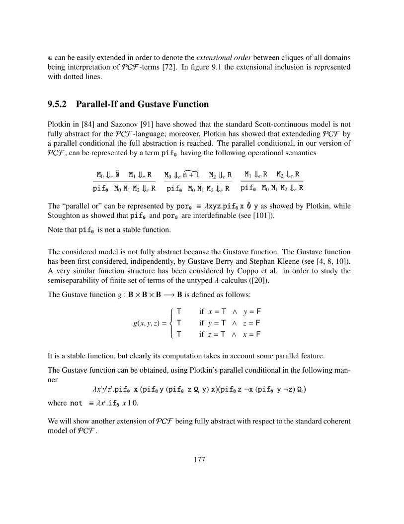
b can be easily extended in order to denote the extensional order between cliques of all domainsbeing interpretation of PCF -terms [72]. In figure 9.1 the extensional inclusion is representedwith dotted lines.

9.5.2 Parallel-If and Gustave Function

Plotkin in [84] and Sazonov [91] have showed that the standard Scott-continuous model is notfully abstract for the PCF -language; moreover, Plotkin has showed that extendeding PCF bya parallel conditional the full abstraction is reached. The parallel conditional, in our version ofPCF , can be represented by a term pif0 having the following operational semantics

M0 ⇓e 0 M1 ⇓e R

pif0 M0 M1 M2 ⇓e R

M0 ⇓e n + 1 M2 ⇓e R

pif0 M0 M1 M2 ⇓e R

M1 ⇓e R M2 ⇓e R

pif0 M0 M1 M2 ⇓e R

The “parallel or” can be represented by por0 ≡ λxyz.pif0 x 0 y as showed by Plotkin, whileStoughton as showed that pif0 and por0 are interdefinable (see [101]).

Note that pif0 is not a stable function.

The considered model is not fully abstract because the Gustave function. The Gustave functionhas been first considered, indipendently, by Gustave Berry and Stephan Kleene (see [4, 8, 10]).A very similar function structure has been considered by Coppo et al. in order to study thesemiseparability of finite set of terms of the untyped λ-calculus ([20]).

The Gustave function g : B × B × B −→ B is defined as follows:

g(x, y, z) =

T if x = T ∧ y = FT if y = T ∧ z = FT if z = T ∧ x = F

It is a stable function, but clearly its computation takes in account some parallel feature.

The Gustave function can be obtained, using Plotkin’s parallel conditional in the following man-ner

λxιyιzι.pif0 x(pif0 y (pif0 z Ωι y) x

)(pif0 z ¬x (pif0 y ¬z) Ωι

)

where not ≡ λxι.if0 x 1 0.

We will show another extension ofPCF being fully abstract with respect to the standard coherentmodel of PCF .

177

9.5.3 Another Gap

It is interesting to consider some traces of function in (B→ B)→ B as

~λ f oo.tt = (∅,T)~λ f oo.condo ( f (tt) tt) (tt) (Ωo) = ((T,T),T), ((∅,T),T)~λ f oo.condo ( f (Ωo) tt) (tt) (Ωo) = ((∅,T),T)~λ f oo.condo ( f (tt) f (tt)) (tt) (Ωo) = ((T,T),T), ((T,F),T), ((∅,T),T), ((∅,F),T)~λ f oo.condo ( f (Ωo) f (Ωo)) (tt) (Ωo) = ((∅,T),T), ((∅,F),T)

Note that ((T,T),T) and ((T,T),T), ((T,F),T) are traces of stables functions.They are PCF-definable? The answer is NO, since f (Ωo) = Ωo is a not PCF test!The respective pseudo-program would be something like

λ f oo.if f (tt) tt and f (Ωo) = Ωo then tt

λ f oo.if f (tt) f (tt) and f (Ωo) = Ωo then tt

Let b to denote the extensional inclusion as defined in Definition 9.5.6 and let # to denote theexistence of a “semantic test” in order to distinguish differents tokens.

Definition 9.5.7 Let X = (|X|, _X) be a coherent space.a, b ∈ |X| are said semantically separable, denoted a#b, if and only if (a,T), (b,F) ∈ X → B.

It follows some intuitive relations

(T,T) b

#

(∅,T) c

#

(F,T)#

(F,T) ⊆ (T,T), (F,T) b (∅,T)

(T,F) b

#

(∅,F) c (F,F)#

(F,F) ⊆ (T,F), (F,F) b (∅,F)

Two token are (semantically) separable if and only if their union is not a clique, namely theycontain at least two incoherent tokens.

9.5.4 Non-Scott-Continuous Stable Functions

Definitions of Scott Domains are standard in literature (as lattices, posets, neighbourhood sys-tems, information systems, ...), so they are not explicitely recalled here [4, 6, 92, 93].

178

Let [B], [B → B] be respectively, standard Scott Domains for booleans and continous arrowsfrom booleans to booleans. It is easy to check that [B] and [B → B] have a finite number ofelements, further there is an isomorphism between they and respectively the posets Cl(B) andCl(B→ B).

Let [B → (B → B)] the standard Scott Domain of continous arrows from [B] to [B → B]. It iswell known that, there is an injection from Cl(B → (B → B)) to [B → (B → B)] but there isno bijection between they, i.e. elements of Cl(B → (B → B)) are strictly less than elements of[B→ (B→ B)].

Now, let [(B → B) → B] the standard Scott Domain of continous arrows from [B → B] to[B]. It would be natural waiting for a relations similar to that showed before in this case too,nevertheless some unexpected fact becomes.

On a first hand, a Scott continous function as λ f oo.pif0 f (tt)tt f (ff) realizing a “parallel or”on f (tt) and f (ff), clearly it’s not a stable function.

But on the oher hand, there are stable functions that are not Scott continous!Note that in the coherent space B→ B the tokens (T,T) and (∅,T) are incoherent; they representrespectively the functions λxo.cond x tt Ωo and λxo.tt.

Let us consider ((T,T)︸ ︷︷ ︸

B→B

, T),((∅,T)︸ ︷︷ ︸

B→B

, F)

it is easy to check that this clique belong to Cl((B → B) → B), since the incoherence between(T,T) and (∅,T) makes true the coherence constraints in the upper level.

Theorem 9.5.8 There are stable functions that are not Scott continous functions.

In particular, this implies that it is not possible to represent stable functions by adding to thelanguage ofPCF only gustave-like functions, since they are Scott-continous and Scott-continousmorphisms are closed under composition.

9.6 Syntax of StPCFIn order to fill the gap between the PCF functions and the morphisms on coherent spaces be-ing interpretations of some PCF -type, we will introduce a nondeterministic conditional and a“control test” function. PCF extended in this manner will be called “stable PCF ” or simplyStPCF .

179

The nondeterministic conditional 3cond has type:

B ` 3cond : ι⇒ ι⇒ ι︸ ︷︷ ︸conditions

⇒ ι⇒ ι⇒ ι︸ ︷︷ ︸branches

⇒ ι

while its execution, corresponding to that of the Gustave function, may be described by thefollowing reduction rules

3cond 0 n P ; M0 M1 M2 →e M0

3cond P 0 n ; M0 M1 M2 →e M1

3cond n P 0 ; M0 M1 M2 →e M2

where n , 0

P0 →e Q0 P1 →e Q1 P2 →e Q2

3cond P0 P1 P2 ; M0 M1 M2 →e 3cond Q0 Q1 Q2 ; M0 M1 M2

Plotkin has showed that if0 p y z can be replaced by pif0 p (pif0 p xΩι) (pif0 pΩι z); never-

theless, note that if0 p y z can be replaced also by

3cond p 1 0 ; y Ωι z .

The “control test” make us able to observing if a programs terminating use or not a ground input.Our “control test” seems to be very similar, although simpler, to that presented by Cartwright,Curien and Felleisen in [17].

test? will be an operator typed as follows

B ` test? : (ι ι) ι

Unfortunately the reduction rule describing the semantics of test? are not intuitive, thus itspresentation will be given first in denotational way

F (~test?ρ) x =

0 if F (x)0 , ∅ and F (x)∅ = ∅1 if F (x)∅ , ∅ (hence, F (x)0 , ∅).∅ otherwise.

180

where x ∈ Cl(N⇒ N). As simple examples,

~test? (λxι.tt)ρ = 1~test? (λxι.if0 x 3 0)ρ = 0~test? (λxι.if0 xΩι 0)ρ = ∅~test? succ ρ = 0~test? pred ρ = ∅ since, by definition ~pred 0ρ = ∅

In order to better understand the function test? some further enlightening, by showing theStPCF -representation of some stable function non PCF -representable:

• the trace ((0, 1), 3) is represented by the StPCF -program

λfιι.if0 (test? f) (if0 (f0) Ωι 3) Ωι;

• the trace ((1, 0), 2), ((∅, 0), 3) is represented by the StPCF -program

λfιι.if0 (((test? (λxι.f(succ x))))) (((if0 (f1) 2Ωι))) (((if0 (fΩι) 3Ωι))).

Definition 9.6.1 (StPCF -words)The words of StPCF are defined by the following grammar:

M ::= x | (λxσ.N) | (PQ) | Yσ

| if0 | succ | pred | n

| test? | 3cond

where x ∈ Var and σ is a type, while M, N, P, Q, ... are metavariables ranging over the wordsof PCF and n, m, ... are metavariables ranging over numerals, namely the numerable constants0, 1, 2, ......

Types of StPCF are that of PCF , FV(3cond) = FV(test?) = ∅, the terms can be obtainedby adding the typing-rules of 3cond and test? to that of the Definition 9.1.5. The contextsextension is straightforward and so that of operational equivalence.

Yet, it is straightforward how test? and 3cond can be transformed for the the language PCF+++B,in order to take in account the booleans.

181

9.6.1 Structured Operational Semantics

Although the operational semantics for this kind of “test” can be formalised by introducing somereduction rule, for sake of simplicity, only an operational presentation in SOS-style will be done.

Definition 9.6.2 Let ⇓e be the relation associating programs to numerals (actually extendingthat defined for PCF ) defined through the formal system proving judgments of the shape

M ⇓e n

and defined by the following rules:

P[Q/x]M1...Mm ⇓e n (m ≥ 0)(head)

(λxσ.P)QM1...Mm ⇓e n

M(YσM) ⇓e n(Y)

YσM ⇓e n

M ⇓e 0 M1 ⇓e n(0if0 )

if0 M0 M1 M2 ⇓e n

M ⇓e k + 1 M2 ⇓e n(1if0 )

if0 M0 M1 M2 ⇓e n

M ⇓e n + 1(pred )

pred M ⇓e n

M ⇓e n(succ )

succ M ⇓e n + 1

(num)n ⇓e n

P0 ⇓e 0 P1 ⇓e k + 1 M0 ⇓e n(03cond)

3cond P0 P1 P2 ; M0 M1 M2 ⇓e n

P1 ⇓e 0 P2 ⇓e k + 1 M1 ⇓e n(13cond)

3cond P0 P1 P2 ; M0 M1 M2 ⇓e n

P1 ⇓e 0 P0 ⇓e k + 1 M2 ⇓e n(23cond)

3cond P0 P1 P2 ; M0 M1 M2 ⇓e n

The operational behavior of test? M is a little bit complex; morally, test? can be describedwith the two following rules:

1. if M0 ⇓e and MΩι ⇑e then test?M ⇓e 0;

2. if M0 ⇓e and MΩι ⇓e then test?M ⇓e 1.

182

Nevertheless, a more constructive operational description can be given.For sake of simplicity, in what follows n0 or n1 will be an abbreviation for the numerals k, if itexists, such that if0 n0 (if0 n1 0 0) n1 ⇓e k (note that if0 n0 0 n1 ⇓e k is equivalent under thehypothesis that n0, n1 are both defined).

test? (P[Q/x]M1...Mm) ⇓e n (m ∈ )(?head)

test?((λxσ.P)QM1...Mm) ⇓e n

test? (M(YσM)) ⇓e n(?Y)

test? (YσM) ⇓e n

test? (λxι.P[Q/z]M1...Mm) ⇓e n (m ≥ 0)(λ?head)

test? (λxι.(λzσ.P)QM1...Mm) ⇓e n

test? (λxι.M(YσM)) ⇓e n(λ?Y)

test? (λxι.(YσM)) ⇓e n

M0 ⇓e 0 M1 ⇓e n(?0if0 )

test? (if0 M0 M1) ⇓e 1

M0 ⇓e k + 1(?1if0 )

test? (if0 M0 M1) ⇓e 0

M0[0/x] ⇓e 0 test? (λxι.M0) ⇓e n0 test? (λxι.M1) ⇓e n1(λ?0if0 )

test? (λxι.if0 M0 M1 M2) ⇓e n0 or n1

M0[0/x] ⇓e k + 1 test? (λxι.M0) ⇓e n0 test? (λxι.M2) ⇓e n2(λ?1if0 )

test? (λxι.if0 M0 M1 M2) ⇓e n0 or n2

M[0/x] ⇓e m + 1 test? (λxι.M) ⇓e n(λ?pred )

test? (λxι.pred M) ⇓e n

(?succ )test? succ ⇓e 0

test? (λxι.M) ⇓e n(λ?succ )

test? (λxι.succ M) ⇓e n

(λ?num)test? (λxι.n) ⇓e 1

(λ?x)test? (λxι.x) ⇓e 0

test? (λxι.(M 0)) ⇓e n(λ??)

test? (λxι.test? M) ⇓e n

P2 ⇓e 0 P0 ⇓e k + 1(?23cond)

test? (3cond P0 P1 P2 M0 M1) ⇓e 0

P0 ⇓e 0 P1 ⇓e k + 1 M0 ⇓e n(?03cond)

test? (3cond P0 P1 P2 M0 M1) ⇓e 1

P1 ⇓e 0 P2 ⇓e k + 1 M1 ⇓e n(?13cond)

test? (3cond P0 P1 P2 M0 M1) ⇓e 1

183

test? (λxι.M0) ⇓e n0

P0[0/x] ⇓e 0 test? (λxι.P0) ⇓e n1

P1[0/x] ⇓e k + 1 test? (λxι.P1) ⇓e n2(λ?03cond)

test? (λxι.3cond P0 P1 P2 ; M0 M1 M2 ) ⇓e n0 or n1 or n2

test? (λxι.M1) ⇓e n0

P1[0/x] ⇓e 0 test? (λxι.P1) ⇓e n1

P2[0/x] ⇓e k + 1 test? (λxι.P2) ⇓e n2(λ?13cond)

test? (λxι.3cond P0 P1 P2 ; M0 M1 M2 ) ⇓e n0 or n1 or n2

test? (λxι.M2) ⇓e n0

P2[0/x] ⇓e 0 test? (λxι.P2) ⇓e n1

P0[0/x] ⇓e k + 1 test? (λxι.P0) ⇓e n2(λ?23cond)

test? (λxι.3cond P0 P1 P2 ; M0 M1 M2 ) ⇓e n0 or n1 or n2

The next theorem gives the basic operational characterization of test?.

Theorem 9.6.3

i) If M[0/z] is a program and M[0/z] ⇓e n then test?(λzι.M) ⇓e k where k ∈ 0, 1; moreover, ifM[Ωι/z] ⇓e n

′ then k ≡ 1 and n′ ≡ n.

ii) If M0 is a program and M0 ⇓e n then test?M ⇓e k where k ∈ 0, 1; moreover, if MΩι ⇓e n′

then k ≡ 1and n′ ≡ n.

iii) If test?M ⇓e k then k ∈ 0, 1 and M0 ⇓e n; moreover, if k ≡ 1 then MΩι ⇓e n.

Proof.

i) The proof is given by induction on the derivation proving M[0/z] ⇓e n.

• If the derivation ends with(P[Q/x])[0/z]M1[0/z]...Mm[0/z] ⇓e n (m ≥ 0)

(head)(λxσ.P)[0/z]Q[0/z]M1[0/z]...Mm[0/z] ⇓e n

then test?(λzι.P[Q/x]M1...Mm) ⇓e k where k ∈ 0, 1, by induction.Thus test?(λzι.((λxσ.P)QM1...Mm)) ⇓e k, by rule (λ?head).If (λxσ.P)[Ωι/z]Q[Ωι/z]M1[Ωι/z]...Mm[Ωι/z] ⇓e n

′ then the last applied rule must be (head),so (P[Q/x])[Ωι/z]M1[Ωι/z]...Mm[Ωι/z] ⇓e n

′ too. Hence k ≡ 1 and n′ ≡ n by induction, sothe proof is immediate.

184

• If (Y) is the last applied rule then the proof follows the guideline of the previous case,byreplacing the rules (λ?head) and (head) respectively by the rules (λ?Y) and (Y).

• If the derivation ends withM[0/z] ⇓e 0 M1[0/z] ⇓e n

(0if0 )if0 M0[0/z] M1[0/z] M2[0/z] ⇓e n

then test?(λzι.M0) ⇓e k0 and test?(λzι.M1) ⇓e k1 where k0, k1 ∈ 0, 1, by induction.Thus test?(λzι.if0 M0 M1 M2) ⇓e k where k ∈ 0, 1 by rule (λ?0if0 ).If if0 M0[Ωι/z] M1[Ωι/z] M2[Ωι/z] ⇓e n

′ then the last applied rule must be either (0if0 ) or(1if0 ), so M0[Ωι/z] ⇓e, thus M0[Ωι/z] ⇓e 0 and k0 ≡ 1 by induction.Hence the last applied rule must be (0if0 ) and M1[Ωι/z] ⇓e n

′, thus n′ ≡ n and k1 ≡ 1 byinduction. But if0 1 (if0 1 0 0) 1 ⇓e 1 implies k ≡ 1.

• If (1if0 ) is the last applied rule then the proof is similar to the previous case.

• If the derivation ends withM[0/z] ⇓e n + 1

(pred )pred M[0/z] ⇓e n

then test?(λzι.M) ⇓e k where k ∈ 0, 1, by induction; so test?(λzι.pred M) ⇓e k by rule(λ?pred ).If pred M[Ωι/z] ⇓e n

′ then M[Ωι/z] ⇓e n′ + 1, since the last applied rule must be (pred );the proof follows by induction.

• If (succ ) is the last applied rule then the proof follows the guideline of the previous case,byrule (λ?succ ).

• Let (num) be the last applied rule; since M[0/z] is a program then either M ≡ z or M ≡ m, forsome numerals m.In the first case z[0/z] ⇓e and z[Ωι/z] ⇑e, but test?(λzι.z) ⇓e 0 by rule (λ?x).In the other case m[0/z] ⇓e m and m[Ωι/z] ⇓e m, but test?(λzι.n) ⇓e 1 by rule (λ?num).

• In case (03cond), (13cond) or (23cond) are the last applied rules then the proof is similar tothe case (0if0 ), respectively by using rules (λ?03cond), (λ?13cond) and (λ?23cond).

• If the derivation ends with

test? ((P[Q/x])[0/z]M1[0/z]...Mm[0/z]) ⇓e n (m ∈ )(?head)

test?((λxσ.P)[0/z]Q[0/z]M1[0/z]...Mm[0/z]) ⇓e n

then test?(λzι.test? (P[Q/x]M1...Mm)) ⇓e k where k ∈ 0, 1, by induction; but the lastrule of the derivation proving test?(λzι.test? (P[Q/x]M1...Mm)) ⇓e k must be (λ??), sotest?(λzι.P[Q/x]M1...Mm0) ⇓e k. So test?(λzι.(λxσ.P)QM1...Mm0) ⇓e k by rule (λ?head),therefore test?(λzι.test?((λxσ.P)QM1...Mm)) ⇓e k by rule (λ??).If test?((λxσ.P)[Ωι/z]Q[Ωι/z]M1[Ωι/z]...Mm[Ωι/z]) ⇓e n′ then the last applied rule must

185

be (?head), so test?((P[Q/x])[Ωι/z]M1[Ωι/z]...Mm[Ωι/z]) ⇓e n′ too. Hence k ≡ 1 andn′ ≡ n by induction, so the proof is immediate.

• If (?Y) is the last applied rule then the proof follows the guideline of the previous case,byreplacing the rules (λ?head) and (?head) respectively by the rules (λ?Y) and (?Y).

• If the derivation ends with

test? (λxι.(P[Q/y])[0/z]M1[0/z]...Mm[0/z]) ⇓e n (m ≥ 0)(λ?head)

test? (λxι.(λyσ.P)[0/z]Q[0/z]M1[0/z]...Mm[0/z]) ⇓e n

then test?(λzι.test? (λxι.(P[Q/y])M1...Mm)) ⇓e k where k ∈ 0, 1, by induction; butthe last rule of the derivation proving test?(λzι.test? (λxι.(P[Q/y])M1...Mm)) ⇓e k mustbe (λ??), so test?(λzι.(((λxι.(P[Q/y])M1...Mm)))0) ⇓e k where the last applied rule must be(λ?head), so test?(((λzι.(P[Q/y])[0/x]M1[0/x]...Mm[0/x]))) ⇓e k.By applying the rule (λ?head), both test?(((λzι.(λyσ.P)[0/x]Q[0/x]M1[0/x]...Mm[0/x]))) ⇓e k

and test?(((λzι.(λxι.(λyσ.P)QM1...Mm)0))) ⇓e k.Thus test?(((λzι.test?(λxι.(λyσ.P)QM1...Mm)))) ⇓e k by rule (λ??).If test?(λxι.(λyσ.P)[Ωι/z]Q[Ωι/z]M1[Ωι/z]...Mm[Ωι/z]) ⇓e n′ then the last applied rulemust be (λ?head), so test?(λxι.(P[Q/y])[Ωι/z]M1[Ωι/z]...Mm[Ωι/z]) ⇓e n′ too. Hencek ≡ 1 and n′ ≡ n by induction, so the proof is immediate.

• If (λ?Y) is the last applied rule then the proof is similar to that of the previous case.

• If (?0if0 ) is the last applied rule then the proof is easier than that of next case.

• If the derivation ends withM0[0/x] ⇓e n + 1

(?1if0 )test? (if0 M0[0/x] M1[0/x]) ⇓e 0

then test?(λzι.M0) ⇓e k where k ∈ 0, 1, by induction; but test?(λzι.0) ⇓e 1 by rule(λ?num). Hence test?(λzι.if0 M0 M10) ⇓e k or 1 by rule (λ?1if0 ).Thus test?(λzι.test? (if0 M0 M1)) ⇓e k or 1 by rule (λ??).If test?(if0 M0[Ωι/x] M1[Ωι/x]) ⇓e n′ then the last applied rule must be (?1if0 ), so theproof follows by induction.

• If the derivation ends with

M0[0/x, 0/z] ⇓e 0 test? (λxι.M0[0/z]) ⇓e n0 test? (λxι.M1[0/z]) ⇓e n1(λ?0if0 )

test? (λxι.if0 M0[0/z] M1[0/z] M2[0/z]) ⇓e n0 or n1

then test?(λzι.test? (λxι.M0)) ⇓e k0 and test?(λzι.test? (λxι.M1)) ⇓e k1 where k0, k1 ∈0, 1, by induction; in both those derivations the last applied rule must be (λ??), sotest?(λzι.(λxι.M0)0) ⇓e k0 and test?(λzι.(λxι.M1)0) ⇓e k1 and yet test?(λzι.M0[0/x]) ⇓e

186

k0 and test?(λzι.M1[0/x]) ⇓e k1 by rule (λ?head).So test? (λzι.if0 M0[0/x] M1[0/x] M2[0/x]) ⇓e k0 or k1 by rule (λ?0if0 ) and, moreover,test? (λzι.(λxι.if0 M0 M1 M2)0) ⇓e k0 or k1 by rule (λ?head).Therefore test? (λzι.test?(λxι.if0 M0 M1 M2)) ⇓e k0 or k1 by rule (λ??).If test?(λxι.if0 M0[Ωι/z] M1[Ωι/z] M2[Ωι/z]) ⇓e n′ then the last applied rule must be(λ?0if0 ), so the proof follows by induction.

• If (λ?1if0 ) is the last applied rule then the proof is similar to that of case (λ?0if0 ).

• If the derivation ends withM[0/x, 0/z] ⇓e n + 1 test? (λxι.M[0/z]) ⇓e n

(λ?pred )test? (λxι.pred M[0/z]) ⇓e n

then test? (λzι.test? (λxι.M)) ⇓e k where k ∈ 0, 1, by induction. But the last rule of thederivation must be (λ??), so test? (λzι.(λxι.M)0) ⇓e k, where the last rule of the derivationmust be (λ?head), so test? (λzι.M[0/x]) ⇓e k.Hence test? (λzι.pred M[0/x]) ⇓e k by rule (λ?pred ), so test? (λzι.(λxι.pred M)0) ⇓e k

by rule (λ?head), thus test? (λzι.test?(λxι.pred M)) ⇓e k by rule (λ??).If test? (λxι.pred M[Ωι/z]) ⇓e n

′ then the last applied rule must be (λ?pred ), so the proofis immediate by induction.

• Let (?succ ) be the last applied rule. FV(test? succ ) = ∅ implies test? succ [Ωι/z] ⇓e.The following derivation is the proof:

(λ?num)test? (λzι.0) ⇓e 1

(λ?succ )test? (λzι.succ 0) ⇓e 1

(λ??)test? (λzι.test? succ ) ⇓e 1

• If the derivation ends withtest? (λxι.M[0/z]) ⇓e n

(λ?succ )test? (λxι.succ M[0/z]) ⇓e n

then test? (λzι.test? (λxι.M)) ⇓e k where k ∈ 0, 1, by induction. But the last rule of thederivation must be (λ??), so test? (λzι.(λxι.M)0) ⇓e k where the last rule of the derivationmust be (λ?head), so test? (λzι.M[0/x]) ⇓e k.Hence test? (λzι.succ M[0/x]) ⇓e k by rule (λ?succ ), so test? (λzι.(λxι.succ M)0) ⇓e k

by rule (λ?head), thus test? (λzι.test?(λxι.succ M)) ⇓e k by rule (λ??).If test? (λxι.succ M[Ωι/z]) ⇓e n

′ then the last applied rule must be (λ?succ ), so the proofis immediate by induction.

187

• Let (λ?num) be the last applied rule. FV(test? (λxι.n)) = ∅ implies test? (λxι.n)[Ωι/z] ⇓e.The following derivation is the proof:

(λ?num)test? (λzι.n) ⇓e 1

(λ?head)test? (λzι.(λxι.n)0) ⇓e 1

(λ??)test? (λzι.test?(λxι.n)) ⇓e 1

• Let (λ?x) be the last applied rule. FV(test?(λxι.x)) implies test?(λxι.x)[Ωι/z] ⇓e. Thefollowing derivation is the proof:

(λ?num)test? (λzι.0) ⇓e 1

(λ?head)test? (λzι.(λxι.x)0) ⇓e 1

(λ??)test? (λzι.test?(λxι.x)) ⇓e 1

• If the derivation ends withtest? (λxι.(M[0/z] 0)) ⇓e n

(λ??)test? (λxι.test? M[0/z]) ⇓e n

then test? (λzι.test? (λxι.(M 0))) ⇓e k where k ∈ 0, 1, by induction. But the last ruleof the derivation must be (λ??), so test? (λzι.(λxι.(M 0))0) ⇓e k where the last rule of thederivation must be (λ?head), so test? (λzι.(M0)[0/x] ) ⇓e k.So test? (λzι.test?(M[0/x])) ⇓e k by rule (λ??), thus test? (λzι.(λxι.test?M)0) ⇓e k byrule (λ?head). Hence test? (λzι.test?(λxι.test?M)) ⇓e k by rule (λ??).If test? (λxι.test? M[Ωι/z]) ⇓e n′ then the last applied rule must be (λ??), thereforetest? (λxι.(M[Ωι/z] 0)) ⇓e n′ too. Hence k ≡ 1 and n′ ≡ n by induction, so the proofis immediate.

• If (?23cond) is the last applied rule then the proof is similar to the case (?1if0 ).

• If (?03cond) or (?13cond) is the last applied rule then the proof is similar to the case (?0if0 ).

• If (λ?03cond), (λ?13cond) or (λ?23cond) is the last applied rule then the proof is similar tothe case (λ?0if0 ).

ii) The proof is given by induction on the derivation proving M0 ⇓e n.Note that M0 is a program implies that M . test? because its type.

• If the last applied rule is (head) then there are two cases.

188

If the derivation ends withP[Q/x]M1...Mm0 ⇓e n (m ≥ 0)

(head)(λxσ.P)QM1...Mm0 ⇓e n

then test?(P[Q/x]M1...Mm) ⇓e k where k ∈ 0, 1, by induction.Thus test?((λxσ.P)QM1...Mm) ⇓e k by rule (λ?head).If (λxσ.P)QM1...MmΩι ⇓e n

′ then the last applied rule must be (head), so (P[Q/x])M1...MmΩι ⇓e

n′ too. Thus k ≡ 1 and n′ ≡ n by induction.

In case the derivation ends withP[0/x] ⇓e n

(head)(λxσ.P)0 ⇓e n

then the proof follows by the point i) of this theorem.

• Let (Y) be the last applied rule. It easy to see that a word Yσ0 cannot be a program, for eachtype σ. If the derivation ends with

N(YσN)0 ⇓e n(Y)

YσN0 ⇓e n

then test? (N(YσN)) ⇓e k where k ∈ 0, 1, by induction, thus the proof follows by rule(?Y). If YNΩι ⇓e n

′ then N(YσN)Ωι ⇓e n′, so the proof follows by induction.

• Let (0if0 ) be the last applied rule; thus the derivation must end with

M ⇓e 0 M1 ⇓e n(0if0 )

if0 M0 M1 0 ⇓e n

so the proof is easy by induction and by rule (?0if0 ).Clearly if0 M0 M1 Ωι ⇓e so the proof is done.

• Let (1if0 ) be the last applied rule; thus the derivation must end with

M ⇓e n + 1 0 ⇓e 0(1if0 )

if0 M0 M1 0 ⇓e n

so the proof is easy by induction and by rule (?1if0 ). Note that if0 M0 M1 Ωι ⇑e.

• The last applies rule cannot be (pred ), since pred 0 ⇑e.

• If (succ ) is the last applied rule then the proof is trivial, by rule (?succ ).Note that succΩι ⇑e.

• The last applies rule cannot be (num).

189

• If (03cond), (13cond) or (23cond) is the last applied rule then the proof follows respectivelyby rule (?03cond), (?13cond), (?23cond).

iii) The proof is given by induction on the derivation proving test?M ⇓e k.

• If the derivation ends withtest? (P[Q/x]M1...Mm) ⇓e k (m ∈ )

(?head)test?((λxσ.P)QM1...Mm) ⇓e k

then k ∈ 0, 1 and P[Q/x]M1...Mm0 ⇓e n by induction, so (λxσ.P)QM1...Mm0 ⇓e n by rule(head). If k ≡ 1 then P[Q/x]M1...MmΩι ⇓e n by induction, so the proof is trivial by rule(head).

• If (?Y) is the last applied rule then the proof is similar to that of the previous case.

• If the derivation ends withtest? (λxι.P[Q/z]M1...Mm) ⇓e k

(λ?head)test? (λxι.(λzσ.P)QM1...Mm) ⇓e k

then k ∈ 0, 1 and (λxι.P[Q/z]M1...Mm)0 ⇓e n by induction, for some n. But the last ap-plied rule in the derivation proving (λxι.P[Q/z]M1...Mm)0 ⇓e n must be (head), having haspremise (P[Q/z])[0/x]M1[0/x]...Mm[0/x] ⇓e n.So both (λzσ.P)[0/x]Q[0/x]M1[0/x]...Mm[0/x] ⇓e and (λxι.(λzσ.P)QM1...Mm)0 ⇓e by rule(head).If k ≡ 1 then (λxι.P[Q/z]M1...Mm)Ωι ⇓e n by induction, but the last applied rule must be(head), having has premise (P[Q/z])[Ωι/x]M1[Ωι/x]...Mm[Ωι/x] ⇓e n. The proof follows byapplying the rule (head) twice.

• If (λ?Y) is the last applied rule then the proof is similar to that of the previous case.

• If the derivation ends withM0 ⇓e 0 M1 ⇓e n

(?0if0 )test? (if0 M0 M1) ⇓e 1

then the proof is easy, since both if0 M0M10 ⇓e n and if0 M0M1Ωι ⇓e n by hypothesis andby rule (0if0 ).

• If (?1if0 ) is the last applied rule then the proof is easy, since 0 ⇓e 0 by rule (num).Thus if0 M0M10 ⇓e 0 by hypothesis and by rule (1if0 ). Note that if0 M1M2Ωι ⇑e.

• If the derivation ends with

M0[0/x] ⇓e 0 test? (λxι.M0) ⇓e k0 test? (λxι.M1) ⇓e k1(λ?0if0 )

test? (λxι.if0 M0 M1 M2) ⇓e k0 or k1

then (λxι.M0)0 ⇓e n0, (λxι.M1)0 ⇓e n1 and k0, k1 ∈ 0, 1 by induction.Since if0 k0 (if0 k1 0 0) k1 ⇓e k0 or k1, it is easy to see that k0 or k1 ∈ 0, 1. But the last

190

rule applied in the derivation proving (λxι.M1)0 ⇓e n1 must be (head), having has premiseM1[0/x] ⇓e n1. Note that M0[0/x] ⇓e 0 by hypothesis; thus if0 M0[0/x] M1[0/x] M2[0/x] ⇓e

n1 by rule (0if0 ), so (λxι.if0 M0 M1 M2)0 ⇓e n1 by rule (head).Moreover, if if0 k0 (if0 k1 0 0) k1 ⇓e 1 then k0 ≡ k1 ≡ 1; so (λxι.M0)Ωι ⇓e n0 and(λxι.M1)Ωι ⇓e n1. Hence M1[Ωι/x] ⇓e n1 by rule (head). Since M0[0/x] ⇓e 0 by hypothesis,M0[Ωι/x] ⇓e 0 by the point i of this theorem. So if0 M0[Ωι/x] M1[Ωι/x] M2[Ωι/x] ⇓e n1 byrule (0if0 ), thus (λxι.if0 M0 M1 M2)Ωι ⇓e n1 by rule (head).

• If (λ?1if0 ) is the last applied rule then the proof is similar to that of case (λ?0if0 ).

• If the derivation ends withM[0/x] ⇓e m + 1 test? (λxι.M) ⇓e k

(λ?pred )test? (λxι.pred M) ⇓e k

then k ∈ 0, 1 and (λxι.M)0 ⇓e n by induction. The last rule applied proving (λxι.M)0 ⇓e n

must be (head), thus M[0/x] ⇓e n and clearly m + 1 ≡ n.The proof follows by rules (pred ) and (head).If k ≡ 1 then (λxι.M)Ωι ⇓e n by induction, but the last applied rule must be (head), havinghas premise M[Ωι/x] ⇓e n. The proof follows by the point i of this Theorem, reasoning asbefore.

• If (λ?succ ) is the last applied rule then the proof is similar to that of case (λ?pred ).

• If the last applied rule is one of the following

(?succ )test? succ ⇓e 0

(λ?num)test? (λxι.n) ⇓e 1

(λ?x)test? (λxι.x) ⇓e 0

then the proof is trivial.

• If the last applied rule istest? (λxι.M 0) ⇓e n

(λ??)test? (λxι.test? M) ⇓e n

then (λxι.M 0)0 ⇓e and n ∈ 0, 1 by induction. Thus M[0/x]0 ⇓e, so by point ii of thistheorem test?M[0/x] ⇓e k where k ∈ 0, 1; so (λxι.test? M)0 ⇓e by rule (head).If k ≡ 1 then (λxι.M 0)Ωι ⇓e by induction, but the last applied rule must be (head), havinghas premise M[Ωι/x] 0 ⇓e n. The proof follows by the point i of this Theorem, reasoningas before.

• If (?03cond), (?13cond) or (?23cond) is the last applied rule then the proof is similar to thatof case (?0if0 ).

• If (λ?03cond), (λ?13cond) or (λ?23cond) is the last applied rule then the proof is similar tothat of case (λ?0if0 ).

191

9.7 Interpretation of StPCFSome preliminary property will be considered, before the StPCF interpretation.

If σ is the type of a PCF program then σγ ≡ τ1 ..... τm ι, for some m ≥ 0; let E = ~σbe the corresponding coherent space, in what follows for sake of simplicity its tokens will bewrited simply as (x1; ...; xm; b) where xi ∈ Cl(~τi), for all i ≤ m, and b ∈ |~γ|.

Lemma 9.7.1 Let E ≡ X1 ⇒ ... ⇒ Xm ⇒ N be a coherent space (m ≥ 1), where Xi is theinterpretation of a PCF -type (1 ≤ i ≤ m).If (x1; ...; xm; bx), (y1; ...; ym; by) ∈ E, such that (x1; ...; xm; bx) , (y1; ...; ym; by), then:

∃k ≤ m such that xk ∪ yk < Cl(Xk) if and only if (x1; ...; xm; bx) ^ (y1; ...; ym; by).

Proof. By induction on m.

m = 1 (⇒) Clearly x1 ∪ y1 < Cl(X1) make immediatly (x1, bx) coherent with (y1, by).

(⇐) Let (x1, bx) ^ (y1, by). Since Cl(N) is flat, bx, by must be in one of the two followingrelations:

a) bx = by implies x1 , y1, since (x1, bx) , (y1, by) by hypothesis, so x1 ∪ y1 < Cl(X1);

b) bx _ by implies, immediately x1 ∪ y1 < Cl(X1).

m ≥ 2 (⇒) If x1 ∪ y1 < Cl(X1) then the proof is trivial.Let x1 ∪ y1 ∈ Cl(X1); by hypothesis there exists k ≥ 2 such that xk ∪ yk < Cl(Xk), so byinduction (x2; ...; xm; bx) ^ (y2; ...; ym; by) and the proof follows by coherence definition.

(⇐) Let (x1; ...; xm; bx) ^ (y1; ...; ym; by). If x1 ∪ y1 < Cl(X1) then the proof is trivial.If x1∪y1 ∈ Cl(X1) then (x2; ...; xm; bx) _ (y2; ...; ym; by) by coherence conditions, thus thereare two cases:

a) (x2; ...; xm; bx) = (y2; ...; ym; by) would imply x1 = y1 by coherence conditions, therefore(x1; ...; xm; bx) = (y1; ...; ym; by) against the hypothesis;

b) the case (x2; ...; xm; bx) ^ (y2; ...; ym; by) follows by induction.

192

Let E ≡ X1 ⇒ ... ⇒ Xm ⇒ N be a coherent space, where Xi is the interpretation of a PCF -type(i ≤ m). If (x1; ...; xm; bx), (y1; ...; ym; by) ∈ E then, as a corollary, it follows:∀k ≤ m, xk ∪ yk ∈ Cl(Xk) if and only if (x1, ...xm, bx) _ (y1, ...ym, by).

Let E ≡ X1 ⇒ ... ⇒ Xm be a coherent space (m ≥ 1), where Xi is the interpretation of a PCF -type (i ≤ m) and t ∈ E; F∗(t) : Cl(X1)&.....&Cl(Xm−1) −→ Cl(Xm) will be the function such that∀xi ∈ Cl(Xi),

F∗(t)x1.....xm = b ∈ |Xm| | ∃(y1, ...ym, b) ∈ t such that ∀i ≤ m, yi ⊆ xi.

Lemma 9.7.2 If M0...Mm is a term (m ≥ 1) then ~M0...Mmρ = F∗(~M0ρ)~M1ρ...~Mmρ.

Proof. By induction on m. If m = 1 then the proof is trivial, in fact

~M0M1ρ = F (~M0ρ)~M1ρ = b | ∃(y, b) ∈ ~M0ρ ∧ y ⊆ ~Mmρ = F∗(~M0ρ)~M1ρ.

Let m ≥ 2; but ~M0...Mm−1ρ = F∗(~M0ρ)~M1ρ...~Mm−1ρ by induction, so

~M0...Mmρ = F (~M0...Mm−1ρ)~Mmρ = b | ∃(ym, b) ∈ ~M0...Mm−1ρ ∧ ym ⊆ ~Mmρ =

b | ∃(ym, b) ∈ F∗(~M0ρ)~M1ρ...~Mm−1ρ ∧ ym ⊆ ~Mmρ =

b | ∃(ym, b) ∈ c | ∃(y1, ...ym−1, c) ∈ ~M0ρ such that ∀i ≤ m − 1, yi ⊆ ~Miρ ∧ ym ⊆ ~Mmρ =

b | ∃(y1, ...ym−1, ym, b) ∈ ~M0ρ such that ∀i ≤ m, yi ⊆ ~Miρ = F∗(~M0ρ)~M1ρ....~Mmρ.

Now the denotational interpretation of StPCF , can be taken in account.

The interpretation of 3cond can be done as follows:

~3condρ = (0; n + 1; ∅; a; ∅; ∅; a) | a ∈ |N| ∪ (∅; 0; n + 1; ∅; a; ∅; a) | a ∈ |N| ∪ (n + 1; ∅; 0; ∅; ∅; a; a) | a ∈ |N|

It is easy that the interpretation is well posed, and in particular that the tokens of this interpreta-tion are coherents.

The interpretation of test? can be done as follows:

193

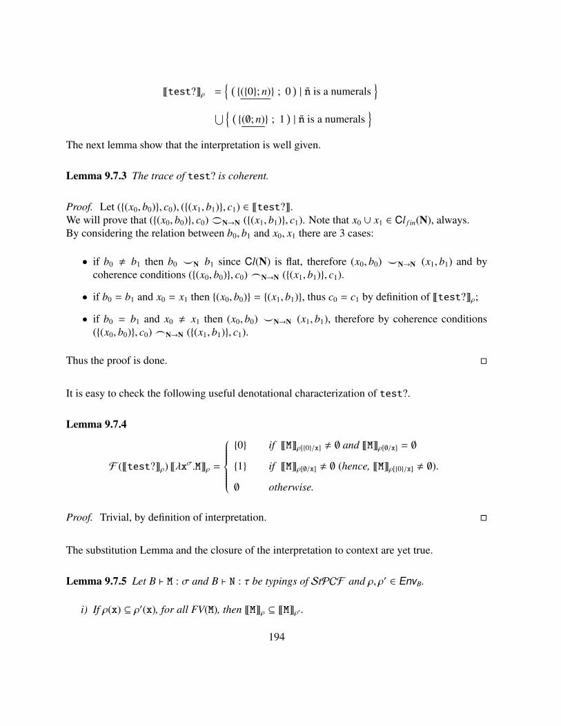
~test?ρ = ( (0; n) ; 0

) | n is a numerals

⋃ ( (∅; n) ; 1) | n is a numerals

The next lemma show that the interpretation is well given.

Lemma 9.7.3 The trace of test? is coherent.

Proof. Let ((x0, b0), c0), ((x1, b1), c1) ∈ ~test?.We will prove that ((x0, b0), c0) _N→N ((x1, b1), c1). Note that x0 ∪ x1 ∈ Cl f in(N), always.By considering the relation between b0, b1 and x0, x1 there are 3 cases:

• if b0 , b1 then b0 _N b1 since Cl(N) is flat, therefore (x0, b0) _N→N (x1, b1) and bycoherence conditions ((x0, b0), c0) ^N→N ((x1, b1), c1).

• if b0 = b1 and x0 = x1 then (x0, b0) = (x1, b1), thus c0 = c1 by definition of ~test?ρ;

• if b0 = b1 and x0 , x1 then (x0, b0) _N→N (x1, b1), therefore by coherence conditions((x0, b0), c0) ^N→N ((x1, b1), c1).

Thus the proof is done.

It is easy to check the following useful denotational characterization of test?.

Lemma 9.7.4

F (~test?ρ) ~λxσ.Mρ =

0 if ~Mρ[0/x] , ∅ and ~Mρ[∅/x] = ∅1 if ~Mρ[∅/x] , ∅ (hence, ~Mρ[0/x] , ∅).∅ otherwise.

Proof. Trivial, by definition of interpretation.

The substitution Lemma and the closure of the interpretation to context are yet true.

Lemma 9.7.5 Let B ` M : σ and B ` N : τ be typings of StPCF and ρ, ρ′ ∈ EnvB.

i) If ρ(x) ⊆ ρ′(x), for all FV(M), then ~Mρ ⊆ ~Mρ′ .

194

ii) If x : τ ∈ B then ~M[N/x]ρ = ~Mρ[ ~Nρ/x].

iii) Let τ = σ and ~Mρ = ~Nρ.If Bc ` C[M] : µ and Bc ` C[N] : µ then ~C[M]ρc = ~C[N]ρc where ρc ∈ EnvBc .

Proof.

i),ii) Similar to the proofs of Lemma 9.4.7.

iii) By induction on C[.]. If C[.] ≡ [.], x, Yν, if0 , succ , pred , 3cond, test?, n then the proofis trivial. If C[.] ≡ C0[.]C1[.] then the proof follows by induction. If C[.] ≡ λxν.C0[.] then

~λxν.C0[M]ρc =

(x0, b) ∈ |~µ|

∣∣∣∣∣∣b ∈ ~C0[M]ρc[x0/x] and∀y ⊆ x0 b ∈ ~C0[M]ρc[y/x] implies y = x0

=

(x0, b) ∈ |~µ|

∣∣∣∣∣∣b ∈ ~C0[N]ρc[x0/x] and∀y ⊆ x0 b ∈ ~C0[N]ρc[y/x] implies y = x0

= ~λxν.C0[N]ρc

A basic link between the operational and the denotational word is stated in the next theorem.

Theorem 9.7.6 Let M be a program. If M ⇓e N then ~Mρ = ~nρ.

Proof. The proof is done by induction on the derivation proving M ⇓e N. When the evaluationinvolves directly the PCF syntax then the proof can be done as in the Theorem 9.4.8. Thus, wecheck only the cases of 3cond and test?.

• If the derivation ends withP0 ⇓e 0 P1 ⇓e k + 1 M0 ⇓e n

(03cond)3cond P0 P1 P2 ; M0 M1 M2 ⇓e n

then by induction ~P0ρ = 0, ~P1ρ = n + 1 and ~M0ρ = n. The proof is trivial, byinterpretation of 3cond.

• If the last applied rule is (13cond) or (23cond) then the proof is similar to that of theprevious case.

• If the derivation ends withtest? (P[Q/x]M1...Mm) ⇓e n (m ∈ )

(?head)test?((λxσ.P)QM1...Mm) ⇓e n

195

then by induction ~test?((λxσ.P)QM1...Mm)ρ = ~nρ and moreover,

~(λxσ.M)Nρ = F (~λxσ.Mρ)~Nρ =

= b | ∃x0 (x0, b) ∈ ~λxσ.Mρ ∧ x0 ⊆ ~Nρ =

= b | ∃x0

(x0, b)

∣∣∣∣∣∣b ∈ ~Mρ[x0/x] and∀y ⊆ x0 b ∈ ~Mρ[y/x] ⇒ y = x0

∧ x0 ⊆ ~Nρ =

= b | b ∈ ~Mρ[~Nρ/x] = ~Mρ[~Nρ/x] = ~M[N/x]ρ

so by Lemma 9.7.5.iii the proof follows.

• If the derivation ends withtest? (λxι.P[Q/z]M1...Mm) ⇓e n (m ≥ 0)

(λ?head)test? (λxι.(λzσ.P)QM1...Mm) ⇓e n

then the proof is similar to that of the previous case.

• If the last applied rule is (?Y) or (λ?Y) then the proof is similar to that of the rule (?head).

• If the derivation ends withM0 ⇓e 0 M1 ⇓e k

(?0if0 )test? (if0 M0 M1) ⇓e 1

then ~M0ρ = 0 and ~M1ρ = k by induction, so it is easy to see that ~if0 M0 M1ρ =

F∗(~if0 ρ)~M0ρ~M1ρ = (∅, k) | n ∈ . The proof follows by interpretation of test?.

• If the derivation ends withM0 ⇓e k + 1

(?1if0 )test? (if0 M0 M1) ⇓e 0

then ~M0ρ = k + 1 by induction; clearly ~if0 M0 M1ρ = F∗(~if0 ρ)~M0ρ~M1ρ =

(m,m) | m ∈ . The proof follows by interpretation of test?.

• If the last applied rule is (λ?0if0 ) then the proof is similar to that of the rule (λ?1if0 ).

• If the derivation ends with

M0[0/x] ⇓e n + 1 test? (λxι.M0) ⇓e n0 test? (λxι.M2) ⇓e n2(λ?1if0 )

test? (λxι.if0 M0 M1 M2) ⇓e n0 or n2

then ~test? (λxι.if0 M0 M1 M2)ρ = F (~test?ρ)~λxι.if0 M0 M1 M2ρ = z.Recall that if0 n0 (if0 n2 0 0) n2 ⇓e k implies that n0 or n2 is k; thus there are three cases.

1. If n0 or n2 ≡ 1 then, both test? (λxι.M0) ⇓e 1 and test? (λxι.M2) ⇓e 1; therefore~test? (λxι.M0)ρ = ~test? (λxι.M2)ρ = 1 by induction.So ~M0ρ[∅/x] , ∅ , ~M2ρ[∅/x], by Lemma 9.7.4. Yet by induction ~M0[0/x]ρ = n+1,so ~M0ρ[0/x] = n + 1 by Lemma 9.7.5.ii and ~M0ρ[∅/x] = n + 1 too. Therefore~if0 M0 M1 M2ρ[∅/x] , ∅ and the proof follows by Lemma 9.7.4.

196

2. If n0 ≡ 0 then test? (λxι.M0) ⇓e 0, so ~M0ρ[∅/x] = ∅ while ~M0ρ[0/x] , ∅; therefore~if0 M0 M1 M2ρ[∅/x] = ∅.Yet by induction ~M0[0/x]ρ = n + 1, so ~M0ρ[0/x] = n + 1. On the other hand,test? (λxι.M2) ⇓e n2 implies ~M2ρ[0/x] , ∅ thus ~if0 M0 M1 M2ρ[0/x] , ∅. The prooffollows by Lemma 9.7.4.

3. If n2 ≡ 0 then test? (λxι.M2) ⇓e 0, so ~M2ρ[∅/x] = ∅ while ~M2ρ[0/x] , ∅. But~M0[0/x]ρ = n + 1 implies, either ~M0ρ[∅/x] = n + 1 or ~M0ρ[∅/x] = ∅; in bothcases ~if0 M0 M1 M2ρ[∅/x] = ∅.Nevertheless ~if0 M0 M1 M2ρ[0/x] , ∅, so by Lemma 9.7.4, the proof is done.

• If the derivation ends withM[0/x] ⇓e m + 1 test? (λxι.M) ⇓e n

(λ?pred )test? (λxι.pred M) ⇓e n

then the proof is similar to that of the case (λ?1if0 ).

• If the derivation ends withtest? (λxι.M) ⇓e n

(λ?succ )test? (λxι.succ M) ⇓e n

then the proof is easy.

• If the last applied rule is one the following

(?succ )test? succ ⇓e 0

(λ?num)test? (λxι.n) ⇓e 1

λ?xtest? (λxι.x) ⇓e 0

then the proof is trivial.

• If the derivation ends withtest? (λxι.M 0) ⇓e n

(λ??)test? (λxι.test? M) ⇓e n

Remark that ~M 0ρ , ∅ if and only if ~test? Mρ , ∅. By Lemma 9.7.4, the proof is easy.

• If the last applied rule is (?23cond) then the proof is similar to that of the rule (?1if0 ).

• If the last applied rule is (?03cond) or (?13cond) then the proof is similar to that of therule (?0if0 ).

• If the last applied rule is (λ?03cond), (λ?13cond) or (λ?23cond) then the proof is similarto that of the rule (λ?0if0 ).

197

9.8 Correctness of StPCFWe will prove first the weak adequacy, hence we will show how the correctness is implied.

We will use the same predicate of the Definition 9.5.2 simply applied to all terms of StPCF .Remember that Comp(∅, M, σ τ) and Comp(∅, N, σ) implies Comp(∅, MN, τ); furthermoreComp(x1 : ν1, ..... , xn : νn, M , τ1 ..... τm ι) (n,m ∈

), Comp(∅, Ni, νi) (1 ≤ i ≤ n),Comp(∅, P j, τ j) (1 ≤ j ≤ m) and

~M[N1/x1, ..., Nn/xn]P1...Pmρ = ~nρ

if and only if M[N1/x1, ..., Nn/xn]P1...Pm ⇓e n.

Lemma 9.8.1 Let B ` M : σ be a valid typing. Always, Comp(B, M, σ).

Proof. The proof is given by induction on the derivation proving B ` M : σ, by considering onlynew typing rules, since the remaining cases can be proved as done in the proof of the Lemma9.5.3.

• Let B ` 3cond : ι ι ι ι ι ι ι and Comp(∅, Ni, ι) (1 ≤ i ≤ 6).Let ~3cond N1 N2 N3 N4 N5 N6ρ = ~nρ. There are 3 cases by 3cond interpretation, weassume without loss of generality, that ~N1ρ = ~0ρ, ~N2ρ = ~k + 1ρ and ~N4ρ = ~nρ.Hence N1 ⇓e 0, N2 ⇓e k + 1 and N4 ⇓e n by hypothesis; thus the proof follows by rule(03cond). The remaining cases are similar.

• Let B ` test? : (ι ι) ι and Comp(∅, N, ι ι).We will show that, if ~test? Nρ = ~nρ then test? N ⇓e n. Clearly both Comp(∅,Ωι, ι)and Comp(∅, 0, ι), so both Comp(∅, NΩι, ι) and Comp(∅, N0, ι) by hypothesis. By interpre-tation of test? there are two cases.

1. If n ≡ 0 then ~NΩιρ = ∅ and ~N0ρ = ~mρ. Hence N0 ⇓e m; moreover test?N ⇓e k

where k ∈ 0, 1 by theorem 9.6.3.ii. If k . 1 then MΩι ⇓e m by Lemma 9.6.3.iii,thus ~NΩιρ = ~mρ , ∅ by Theorem 9.7.6 against our hypothesis.

2. If n . 0 then ~NΩιρ = ~N0ρ = ~mρ. Hence NΩι ⇓e m and N0 ⇓e m; thus the prooffollows by Lemma 9.6.3.ii.

Corollary 9.8.2 Our denotational semantics is weakly adequate.

198

Proof. The Lemma 9.8.1 together with Theorem 9.7.6 implies that ~Mρ = ~nρ if and only ifM ⇓e n, for each programs M, numerals n and environment ρ.

The weak adequacy implies the correctness.

Theorem 9.8.3The given denotational semantics is correct with respect to the operational semantics.

Proof. Let M, N be two terms of PCF and ~Mρ = ~Nρ, for each environment ρ. If C[.] isa context such that both C[M] and C[N] are programs and C[M] ⇓e n, for some value n, then~C[M]ρ = ~nρ by Theorem 9.7.6, so ~C[N]ρ = ~nρ by hypothesis and Lemma 9.7.5, henceC[N] ⇓e n by weak adequacy.By definition of operational equivalence the proof is done.

9.9 Definability and Full Abstraction of StPCFAs done by Plotkin for PCF and Scott-Domains in [84], we will show the that the coherentspaces give us a fully abstract semantics for StPCF by showing the definability of finite cliques,namely if x0 is a finite clique (in an coherent space interpretation of a PCF -type) then there exista StPCF program M such that ~Mρ = x0.

Definition 9.9.1 Let x be a finite clique of a StPCF -term.So PxQ will denote the class of terms having x as in interpretation, namely PxQ = M | ~Mρ = x.

By abusing the notation, if a is a token of a StPCF -term then PaQ will be used in place of PaQand often we will write PxQ = M in place of M ∈ PxQ.

We introduce some notations that we will use everywhere in what follows.As defined in subsection 9.5.1, recall that M N is an abbreviation for the application of thefollowing term to M and N:

` Yιιι

(λFιιιxιyι.if0 x (if0 y01)

(if0 y (if0 x01) (F(pred x)(pred y))

)): ι ι ι.

Furthermore, let n0 or n1 be an abbreviation for the term if0 n0 (if0 n1 0 0) n1, let n0 and n1 bean abbreviation for the term if0 n0 (if0 n1 0 1) (if0 n1 1 1), let not n0 be an abbreviation forthe term if0 n0 1 0, last let k-succ M be an abbreviation for succ .....succ︸ ︷︷ ︸

k

M where k ∈ and M

199

is a term (possibly open) having type ι. Note that or and and are strict operators, in the sensethat if one of their parameters diverges then their evaluation diverges.

In order to help the reader, we will try to give an informal idea of the problems raising in theproof of the definability by observing some examples will be presented.

Example 9.9.2 a) Let (3, 4) ∈ |~ι ι|, so clearly P(3, 4)Q = λxι.if0 (x 3)4Ωι.

b) Let ((3, 4), 5) ∈ |~(ι ι) ι|. At a first sight, the term M ≡ λfιι.if0 (f3 4)5Ωι isa natural candidate for P((5, 6), 3)Q but unfortunately this impression is wrong, in fact~Mρ = ((3, 4), 5), ((∅, 4), 5). It is easy to check that

P((3, 4), 5)Q = λfιι.if0

(f3 4 and

test?(λzι.f(3-succ z))

)5Ωι.

c) Let (((3, 4), 5), 6) ∈ |~((ι ι) ι) ι|.Note that the term M ≡ λF(ιι)ι.if0

(F(λxι.if0 (x 3)4Ωι

) 5

)6Ωι does not define the

considered token, in fact ~Mρ = (((3, 4), 5), 6), ((∅, 5), 6). It is easy to check that

P(((3, 4), 5), 6)Q = λF(ιι)ι.if0

(F(λxι.if0 (x 3)4Ωι

) 5

)and

test?(λzι.F

(λxι.if0 (x 3)(4-succ z)Ωι

)) 6Ωι.

d) Let a ≡ ((((3, 4), 5), 6), 7) ∈ |~(((ι ι) ι) ι) ι|.Note that the term M ≡ λF((ιι)ι)ι.if0

(F(λfιι.if0 ((f3) 4)5Ωι

) 6

)7Ωι does not

define the considered token, in fact

~Mρ = ((((3, 4), 5), 6), 7), ((((∅, 4), 5), 6), 7), ((∅, 6), 7).

By using P((3, 4), 5)Q defined in point b, it is easy to check that

PaQ = λF(ιι)ι.if0

((F P((3, 4), 5)Q

) 6

)and

test?(λfιι.F

(λxι.if0 ((f3) 4)(5-succ z)Ωι

)) 7Ωι.

The following property is crucial key making us able to prove the definability.

Property 9.9.3 Let ` M : σ ι be a StPCF -typing, ~Mρ = f ∈ Cl~σ ι and x ∈ Cl f in~σ.If x = a0, ...., an (n ∈

) and xak = (∅, a0), ..., (0, ak), ..., (∅, an) (k ≤ n) then, the followingpoint are equivalent:

200

i) b ∈ F ( f )x and, ∀y ⊆ x, b ∈ F ( f )y implies x = y;

ii) ∀k ≤ n, F ( f )(((F (xak)0))) = b while F ( f )(((F (xak)∅))) = ∅;iii) b ∈ ~M(PxQρ and, ∀k ≤ n, ~test?(λzι.M(PxakQz))ρ = 0.

Proof. Easy, by using the Lemma 9.7.4.

A further enlightening example follows.

Example 9.9.4

a) Let a ≡ ((10, 11)︸ ︷︷ ︸ιι

; ((3, 4), 5), ((3, 8), 9)︸ ︷︷ ︸(ιι)ι

; 6) ∈ |~(ι ι) ((ι ι) ι) ι|.

Note that the term

M ≡ λfιιF(ιι)ι.if0(f10 11 and (F P(3, 4)Q) 5 and (FP(3, 8)Q) 9

)6Ωι

does not define the considered token a, in fact

~Mρ =

((10, 11); ((3, 4), 5), ((3, 8), 9); 6

)((∅, 11); ((3, 4), 5), ((3, 8), 9); 6

)

It is easy to check that

PaQ = λfιιF(ιι)ι.if0

f10 11 and test?(λzι.f(10-succ z))

(F P(3, 4)Q) 5 and (FP(3, 8)Q) 9

6Ωι.

b) Let e =

((3, 30), (4, 41), 101), ((∅, 90), 109),((3, 31), (5, 50), 102), ((4, 40), (5, 51), 103)

∈ Cl(~(ι ι) ι

).

Let x101 = (3, 30), (4, 41), x102 = (3, 31), (5, 50), x103 = (4, 40), (5, 51),x109 = (∅, 90) and, note that they are pairwise incoherent. We will try to define theclique e in a compositional way, so some simpler cliques is defined first.

P

(x101, 0)(x109, 1)

Q = λfιι.if0

f3 30

and

f4 41

0

(if0

(f90 ˜109 and

not (((test?(λzι.f(90-succ z)))))

)1Ωι

)

201

It wolud be clear that, in case f3 30 and f4 41 there is no need for checking theminimality, since it must be ~fΩιρ = ∅ by monotonicity and correctness.

P

(x101, 1)(x103, 0)(x104, 0)

Q = λfιι.3cond

if0 (f3 30) (if0 (f4 41)0Ωι)(if0

f3 31

and

f5 50

1Ωι)

if0 (f4 40) (if0 (f5 51)0Ωι)(if0

f4 41

and

f3 30

1Ωι)

if0 (f5 50) (if0 (f3 31)0Ωι)(if0

f5 51

and

f4 40

1Ωι)

1

0

0

P

(x109, 0)(x103, 1)(x104, 1)

Q = λfιι.if0 (f5 90)(fΩι 90)if0 (f5 50) (if0 (f3 31)1Ωι)(if0

f5 51

and

f4 40

1Ωι)

Thus it is easy to check that:

PeQ = λfιι.3cond

(P

(x101, 0)(x109, 1)

Q f

) P

(x101, 1)(x103, 0)(x104, 0)

Q f

P

(x109, 0)(x103, 1)(x104, 1)

Q f

˜101

if0 (f5 50) (if0 (f3 31) ˜102Ωι)(if0

f5 51

and

f4 40

˜103Ωι)

˜109

We remark that in the definition of previous cliques there are many part of programs beingredundant, so it can be simplified.

Cl f in(E B⇒ N) will denote the subset of Cl f in(E → N) such that u ∈ Cl f in(E B⇒ N) if and only if(y0, b) ∈ u then, either b = 0 or b = 1.

Lemma 9.9.5Let E ≡ ~σ be a coherent space, such that σ ≡ τ1 ..... τm ι (m ≥ 0) is a type.If e ∈ Cl f in(E) then e is definable.

202

Proof. We will prove that, if e ∈ Cl f in(E) then e is definable and moreover if u ∈ Cl f in(E B⇒ N)then u is definable too. The proof is given by induction on level(σ) (see Definition 9.1.2).q Let level(σ) = 0, namely E = N and σ = ι. Thus Ωι and the numerals n define all possiblefinite clique, since Cl f in(N) = ∅ ∪ n / n ∈ | |.Furthermore, if u ∈ Cl f in(N B⇒ N) then u is definable, by induction on ‖u‖.

• u = ∅ is defined by Ωι→ι.

• Let u = (x1, b1) such that x1 ∈ Cl f in(N) and b1 ∈ 0, 1.If x1 = ∅ then there are just two cases λzι.0, λzι.1. If x1 , ∅ then ‖x1‖ = 1, i.e. it containsa numerals, since Cl(N) is a flat cpo. If x1 = n then the program defining the clique hasthe following shape: λzι.if0 (z n) PbQΩι.

• Let ‖u‖ > 1 and (x1, b1) ∈ u; so x1 ∈ Cl f in(N) and b1 ∈ 0, 1. Clearly x1 , ∅ since Cl(N)is a flat cpo. If u′ = u − (x1, b1) and x1 = n1 then program defining the clique has thefollowing shape: λzι. (((z ι Pn1Q))) Pb1Q (((Pu′Qz))) where Pu′Q is well defined by induction.

q Let level(σ) = l and l ≥ 1, thus σ ≡ τ1 ..... τm ι where m ≥ 1.We will show that each e ∈ Cl(E) is definable, by induction on ‖e‖.

• If e = ∅ then PeQ ≡ Ωσ.

• Let e = a0 where ai = (x1; ...; xm; b) (i ≤ n) and X j = ~τ j (1 ≤ j ≤ m).Clearly (x j, 0) ∈ |X j

B⇒ N| (1 ≤ j ≤ m) are definable by induction, thus

PeQ ≡ λz1...zm.if0(P(x1, 0)Qz1 and .... and P(xm, 0)Qzm

)PbQ Ωι.

• Let e = a0, ....., an where n ≥ 0, ai = (xi1; ...; xi

m; bi) (i ≤ n) and X j = ~τ j (1 ≤ j ≤ m).There exists k ≤ m such that x0

k ∪ x1k < Cl(X1) and in particular, there exists c ∈ x0

k andd ∈ x1

k such that c _Xk d, by Lemma 9.7.1. Therefore

e1 = (xi1; ...; xi

m; bi) ∈ e / c ∈ xik ∈ Cl(Xk)

e2 = (xi1; ...; xi

m; bi) ∈ e / d ∈ xik ∈ Cl(Xk)

e3 = e − (e1 ∪ e2) = (xi1; ...; xi

m; bi) ∈ e / c, d < xik

are definable by induction on the size, while

u1 = (x1; ...; xm; 0) / ∃(x1; ...; xm; b) ∈ e1 ∪ (x1; ..., xm; 1) / ∃(x1; ...; xm; b) ∈ e2u2 = (x1; ...; xm; 0) / ∃(x1; ...; xm; b) ∈ e3 ∪ (x1; ..., xm; 1) / ∃(x1; ...; xm; b) ∈ e1u3 = (x1, ..., xm, 0) / ∃(x1; ...; xm; b) ∈ e2 ∪ (x1; ...; xm; 1) / ∃(x1; ...; xm; b) ∈ e3

are cliques, by Lemma 9.7.1, and they definable by induction on the level. Hence,

PeQ ≡ λz1...zm.3cond (Pu1Qzk) (Pu2Qz1...zm) (Pu3Qz1...zm) ;(Pe1Qz1...zm) (Pe3Qz1...zm) (Pe2Qz1...zm).

203

By induction on ‖u‖ we will check that if u ∈ Cl f in(E B⇒ N) then u is definable too!Note that level(σ) ≥ 1 implies that σ . ι.

• If u = ∅ then the proof is trivial.

• Let u = (e0, bu0) where bu

0 ∈ 0, 1 and reason by induction on ‖e0‖.– If e0 = ∅ then PuQ ≡ λFσ.Pbu

0Q.

– Let e0 = a0 where a0 = (x01; ...; x0

m; b0).We will show that the clique u = ((x0

1; x02; ...; x0

m; b0), bu0) is definable. Note that,

both x0i (i ≤ m) and u′ = ((x0

2; ...; x0m; b0), bu

0) are definable, by induction on level.You can check that M ≡ λFσ.if0

((F Px0

1Q...Px0mQ)

ι Pb0Q)Pbu

0QΩι does not define u;

in fact, ~M =((z1, ..., zm, b0), bu

0) / ∀i ≤ m zi ⊆ x0i

(see Example 9.9.2).

If x01 = c0

1, ..., c0h1 then x

c0j

1 = (∅, c01), ..., (0, c0

j ), ..., (∅, c0h1

) (1 ≤ j ≤ h1) is a cliquedefinable by induction, thus

PuQ ≡ λFσ.if0

((((F Px01Q...Px0

mQ))) ι Pb0Q) and

test?(λxι.F (Pxc0

11 Qx) Px0

2Q...Px0mQ)

and ..... and

test?(λxι.F (Pxc0

h11 Qx) Px0

2Q...Px0mQ)

(Pu′Q(FPx0

1Q))

Ωι.

– Let e0 = a0, ....., an (n ≥ 1) where ai = (xi1; ...; xi

m; bi) (i ≤ n) and Xi = ~τi(1 ≤ i ≤ m). Note that e′ = e − a0 = ((x1

1; ...; x1m; b0), ....., (xn

1; ...; xnm; bn), bu

0)is a clique definable by induction on the size. Let a0 = (x0

1; ...; x0m; b0); so and u′ =

((x02; ...; x0

m; b0), 0) is a clique definable by induction on the level.

If x01 = c0

1, ..., c0h0 then let x

c0k

1 = (∅, c01), ..., (0, c0

k), ..., (∅, c0h0

) (k0 ≤ h0) thus

PuQ ≡ λFσ.if0

((((F Px01Q...Px0

mQ))) ι Pb0Q) and

test?(λxι.F (Pxc0

11 Qx) Px0

2Q...Px0mQ)

and ..... and

test?(λxι.F (Pxc0

h11 Qx) Px0

2Q...Px0mQ)

and (Pu′Q(FPx01Q))

(Pe′QF) Ωι.

• Let u = (e0, bu0), ....., (ep, bu

p) (p ≥ 1) where buj ∈ 0, 1 ( j ≤ p).

By Lemma 9.7.1, if i, j ≤ p and i , j then ei ∪ e j < Cl(E); thus ei , ∅, for each j ≤ p.

Let e j = a j0, ....., a

jn j (n j ≥ 0), a j

i = (x( j,i)1 ; ...; x( j,i)

m ; b( j,i)) (i ≤ n j, j ≤ p) and Xi = ~τi(i ≤ m).

204

There exists a0k0∈ e0 (k0 ≤ n0) and a1

k1∈ e1 (k1 ≤ n1) such that a0

k0_ a1

k1. Let a0

k0≡

(x(0,k0)1 , ..., x(0,k0)

m , b(0,k0)) and a1k1≡ (x(1,k1)

1 , ..., x(1,k1)m , b(1,k1)), therefore x(0,k0)

i ∪ x(1,k1)i ∈ Cl(Xi)

(i ≤ m) are definable, yet by Lemma 9.7.1. So, let zi = x(0,k0)i ∪ x(1,k1)

i (i ≤ m).Furthermore, note that a0

k0, a1

k1imply that b(0,k0) , b(1,k1) or there exists q ≤ m such that

x(0,k0)q , x(1,k1)

q .

Note that the following cliques are definable by induction on the size:

v1 = (ei, bui ) ∈ u / a0

k0∈ ei

v2 = (ei, bui ) ∈ u / a1

k1∈ ei

v3 = u − (v1 ∪ v2) = (ei, bui ) ∈ u / a0

k0< ei and a1

k1< ei

w′1 = (ei, 0) / (ei, bui ) ∈ v1

w′′1 = (ei, 1) / (ei, bui ) ∈ v2

w2 = (ei, 0) / (ei, bui ) ∈ v3 ∪ (ei, 1) / (ei, bu

i ) ∈ v1w3 = (ei, 0) / (ei, bu

i ) ∈ v2 ∪ (ei, 1) / (ei, bui ) ∈ v3

– If b(0,k0) , b(1,k1) then w? = (b(0,k0), 0) , (b(1,k1), 1) is definable, by induction. Hence

PuQ ≡ λFσ.3cond(if0 (((Pw?Q(F Pz1Q...PzmQ))))(Pw′1QF)(Pw′′1 QF)

)(Pw2QF) (Pw3QF)

(Pv1QF) (Pv3QF) (Pv2QF)

– Otherwise b(0,k0) = b(1,k1). Let q ≤ m, such that x(0,k0)q , x(1,k1)

q .Without loss of generality, there is a token c0

q ∈ x(0,k0)q such that c0

q < x(1,k1)q ; in fact, if

such a token does not exist, it is sufficient to exchange (e0, bu0) and (e1, bu

1).

Hence zc0

qq = (0, c0

q) ∪ (∅, c) / c ∈ zq and a , c0q is a clique definable by induction,

and

PuQ ≡ λFσ.3condif0

(F Pz1Q...PzmQ) ι Pb(0,k0)Q and

test?(λxι.FPz1Q...Pzq−1Q(Pz

c0q

q Qx)Pzq+1Q...PzmQ)

(Pw′1QF)(Pw′′1 QF)

(Pw2QF) (Pw3QF)(Pv1QF) (Pv3QF) (Pv2QF).

The definability implies the completeness as showed in the next theorem.

Theorem 9.9.6The given denotational semantics is complete with respect to the operational semantics.

205

Proof. The interpretation of an abstraction is defined as

~λxµ.Pρ =

(x0, b) ∈ Cl f in(~µ) × |~τ|

∣∣∣∣∣∣b ∈ ~Pρ[x0/x] and∀y ⊆ x0 b ∈ ~Pρ[y/x] implies y = x0

for some types µ, τ. It is easy to see that, if M, N are two open terms of PCF such that M / N andFV(M) ∪ FV(N) ⊆ x1, ..., xn then λx1...xn.M / λx1...xn.N.

Let M, N be two closed terms of PCF such that ∅ ` M : σ and ∅ ` N : σ, while M / N.Note that the interpretation is invariant with respect to ρ, since M, N are closed; thus by definition~Mρ , ~Nρ, for each environment ρ.

Let σ ≡ τ1 ..... τm ι (m ≥ 0) and without loss of generality assume that there isa = (x1; ...; xm; b) and x j ∈ X j = ~τ j (1 ≤ j ≤ m) such that a ∈ ~Mρ but a < ~Nρ.

By Lemma 9.9.5, there is a terms Px jQ having x j as interpretation (1 ≤ j ≤ m).Hence by definition of interpretation, clearly ~MPx1Q.....PxmQρ = ~PbQρ while, on the other hand,~NPx1Q.....PxmQρ = ∅ , ~PbQρ by Lemma 9.7.1. Therefore M 0 N, since by Corollary 9.8.2,both MPx1Q.....PxmQ ⇓e PbQ and NPx1Q.....PxmQ ⇑e, and the proof is done.

Hence, ∼ and ≈ are the same relation on programs of StPCF .

Corollary 9.9.7The given denotational semantics is fully abstract with respect to the operational semantics.

Proof. By Theorems 9.8.3 and 9.9.6.

We conjecture that our syntax does not make definable all cliques of coherent spaces (not onlyfinite), thus a first open problem is to find a syntax such that all cliques of coherent spaces aredefinable, as done for Scott-Domains by Plonking.

Other questions are the relations between either strongly stable functions or bidomains withStPCF .

206

Bibliography

[1] Abramsky S., Jagadeesan R., Malacaria P., “Full Abstraction for PCF (extended abstract).”,Lecture Note in Computer Science, Vol.789, 1994.

[2] Abramsky S., Ong L.C., “Full abstraction in the Lazy Lambda Calculus”, Information andComputation, 105, 1993, pp. 159-267.

[3] Aho A.V., Sethi R., Ullman J.D., “Compilers: principles techniques and tools.” Addison-Wesley, 1986.

[4] Amadio R., Curien P.L., “Domains and Lambda-Calculi.”, Cambridge Tracts in TheoreticalComputer Science, N.46, 1998.

[5] Bakel S., Barbanera F., Dezani-Ciancaglini M., Vries F., “Intersection Types for λ-trees”,Theoretical Computer Science, 272, 2002 pp.3-40.

[6] Barendregt H., “The Lambda Calculus: its Syntax and Semantics”, revised edition, NorthHolland, 1984.

[7] Bastonero O., Pravato A., Ronchi Della Rocca S., “Structures for Lazy Semantics”, Pro-gramming Concepts and Methods, Gries and de Roever ed.s, Chaptman & Hall, 1998, pp.30-48.

[8] Berry G., “Modeles completement adequats et stable du lambda-calcul type.”, These de Doc-torat d’Etat, Paris VII, 1979.

[9] Berry G., “Sequentialite de l’evaluation formelle des λ-expressions”, Automata, languagesand programming (3 Int. Coll. Paris), 1978, DUNOD, pp.67-80.

[10] Berry G., “Stable Models of typed lambda-calculi”, Automata, languages and programming(5 Int. Coll. Udine), LNCS 62, 1978, pp.72-89.

[11] Berry G., Curien P.L., Levy J.J., “Full abstraction for sequential languages: state of the art”,Algebraic methods in Semantics, Nivet and reynolds ed.s, Cambridge University Press, 1985,pp. 89-132.

207

[12] Bloom B., “Can LCF be topped? Flat lattice models of typed λ-calculus”, Information andComputation, 87, 1990, pp.263-300.

[13] Bohm C., “Alcune Proprieta’ delle forme βη-normali nel λK-calcolo”, Pubblicazionidell’Istituto per le Applicazioni del Calcolo, 696, 1968.

[14] Bohm C., Dezani-Ciancaglini M., Peretti P, Ronchi Della Rocca S., “A DiscriminationAlgorithm inside λ-calculus”, Theoretical Computer Science, 8, 3,1978, pp. 271-291.

[15] Bucciarelli A., Ehrhard T., “Sequentiality and Strong Stability”, in Proc. 6th Symp. Logicin Computer Science, IEEE press, 1991, pp.138-145.

[16] Bucciarelli A., Ehrhard T., “A theory of sequentiality”, Theoretical Computer Science, 113,1993, pp.273-291.

[17] Cartwright R., Curien P.L., Felleisen M., “Fully Abstract Semantics for observably sequen-tial languages”, Information and Computation, 111, 1994, pp.297-401.

[18] Church A., “The Calculi of lambda-conversion”, Princeton University Press, Princeton, NJ,1941.

[19] Coppo M., Dezani-Ciancaglini M., “An extension of the basic functionality theory for theλ-calculus”, Notre Dame J. Formal Logic, 21(4), 1980, pp.685-693.

[20] Coppo M., Dezani-Ciancaglini M., Ronchi Della Rocca S.: “(Semi)-separability of FiniteSets of terms in Scott’sD∞-Models of the λ-calculus”, International Conference on AutomataLanguages and Programming 1978, Ausiello and Bohm ed.s, Lecture Notes in ComputerScience, 62, Springer-Verlag, 1978, pp. 142-164.

[21] Curien P.L., “Categorical combinators, sequential algorithms and functional program-ming”, Research Notes in Theoretical Computer Science, Pitman, 1986.

[22] Curien P.L., “Abstract Machines, control and sequents.” Coursenotes for theAPPSEM’2000-International summer school on applied sematics. (Available in “http://www-sop.inria.fr/oasis/Caminha00/abstract.html”).

[23] Curien P.L., Herbelin H., “The duality of computation”, Proc. International Conference onFunctional Programming, September 2000, Montreal, IEEE (2000)).

[24] Curry H.B., Feys R. “Combinatory Logic”, vol. 1, North Holland, 1958.

[25] Curry H.B., Hindlley J. R., Seldin J.P. “Combinatory Logic”, vol. 2, Studies in Logic 65,North Holland, 1972.

[26] Danos V., Regnier L., “The structure of multiplicatives.”, Archive for Mathematical Logic,Vol.28, 181-203, 1989.

208

[27] David R., Nour K., “A Syntactical proof of the operational equivalence of two lambdaterms”, Theoretical Computer Science, 180, (1997), pp. 371-375.

[28] Dezani-Ciancaglini M., Honsell F., Alessi F., “A complete characterization of completeintersection-type preorders”, ACM TOCL, 4(1), 2003, pp. 120-147.

[29] Dezani-Ciancaglini M.,Honsell F.,Ronchi Della Rocca S., “Models for theories of Func-tions strictly depending on all their arguments”, (abstract), Journal of Symbolic Logic, 51, 3,(1986), 845-846.

[30] Dezani-Ciancaglini M., Intrigila B., Venturini-Zilli M., “Bohm’s Theorem for BohmTrees”, ICTCS98, World Scientific, Oxford, 1998, pp.1-23.

[31] Di Cosmo R., “ A brief history of rewriting with extensionality”, In Fairouz Kamareddine,editor, International Summer School on Type Theory and Rewriting, Glasgow, September1996, Kluwer.

[32] Egidi L., Honsell F., Ronchi Della Rocca S., “Operational, Denotational and Logical De-scription: a case study”, Fundamenta Informaticae, 16, 2, (1992), pp. 149-170.

[33] Felleisen M., Friedman P.D., “A syntactical Theory of Sequential State”, Theoretical Com-puter Science, 69 (1989), pp. 243-287.

[34] Felleisen M., Friedman P.D., Kohlbecker E., Duba B., “A syntactical Theory of SequentialControl”, Theoretical Computer Science, 52 (1987), pp. 205-237.

[35] Girard J.Y., “The System F of Variable Types, fifteen years later”, Theoretical ComputerScience, 45, 1986, pp. 159-192.

[36] Girard J.Y., “Linear Logic”, Theoretical Computer Science, 50, 1987, pp. 1-102.

[37] Girard J.Y., “Towards a geometry of interaction.”, Categories in Computer Science andLogic, 69-108, 1989.

[38] Girard J.Y., “Geometry of interaction I: interpretation of system F.”, Logic Colloqium 1988,In Ferro, Bonotto, Valentini, Zanardo editors, 1989.

[39] Girard J.Y., “Geometry of interaction II: deadlock-free algorithms.”, Lecture Note in Com-puter Science, In Martin-Lof, Mints editors, Vol.417 76-93,1990.

[40] Girard J.Y., “Geometry of interaction III: accomodating the additives.” Advances in LinearLogic, In Girard, Lafont, Regnier editors, 1995.

[41] Girard J.Y., “On the meaning of logical rules I: syntax vs. semantics.”, ComputationalLogic, In U. Berger and H. Schwichtenberg editors, 1999.

209

[42] Girard J.Y., “ On the meaning of logical rules II: multiplicative/additive case.”, Foundationof Secure Computation, In F. L. Bauer and R. Steinbrggen editors, 2000.

[43] Girard J.Y., “Locus Solus.”, Manuscrit, 1999.

[44] Girard J.Y., “Locus Solum: from the rules of logics to the logics of rules”, MathematicalStructures in Computer Science, 11, 2001, pp.301-506.

[45] Girard J.Y., Lafont Y., Taylor P., “Proofs and Types.”, Cambridge tracts in thoretical com-puter science, Vol.7, 1990.

[46] Gordon M., Milner R., Wadsworth C., “Edinburgh LCF: a mechanized logic of computa-tion”, Lecture Notes in Computer Science, 78, 1979.

[47] Hindley R., “Basic Simple Type Theory”, Cambridge Univ. Press 1995.

[48] Hindley R., Seldin J., “Introduction to Combinators and Lambda-calculus”, CambridgeUniv. Press 1986.

[49] Hindley R., Longo G., “Lambda Calculus Models and Extensionality”, Z. Math. LogikGrundlag. Math., 26, 1980, pp. 289-310.

[50] Honsell, F., Lenisa, M., “Final Semantics for untyped λ-calculus”, LNCS 902, 1995, pp.249-265.

[51] Honsell F., Ronchi Della Rocca S., “An Approximation Theorem for Topological LambdaModels and the Topological Incompleteness of Lambda Calculus”, Journal of Computer andSystems Science, 45, 1992, pp.49-75.

[52] Honsell F., Ronchi Della Rocca S., “Reasoning about Interpretations in Qualitative LambdaModels”, Programming Concept and Methods, Broy and Jones ed.s, North Holland, 1990,pp.505-521.

[53] Hyland Y., “A Syntactic Characterization of the Equality in some Models of the LambdaCalculus”, Journal of London Mathematical Society, 12, 2, 1976, pp.83-95.

[54] Hyland M., Ong. L., “On full abstraction for PCF.”, Technical Report, 1994

[55] Jim T., Meyer A.R., “Full Abstraction and Context Lemma”, SIAM Journal Computing,25(3), 1996, pp.663-696.

[56] Kahn G., “Natural Semantics”, Programming of Future Generation Computers, Fuchi andNivat ed.s, North Holland, 1988, pp.237-257.

[57] Klop J.W., “Combinatory Reduction Systems”, Mathematical Center Tracts 129, 1980,Amsterdam.

210

[58] Krivine J.L., “Lambda-calculus, types and models”, Ellis Horwood (1993).

[59] Landin P.J.,“The mechanical evaluation of expressions”, Comput.J.,6,1963, pp.308-320.

[60] Landin P.J., “A correspondence between ALGOL 60 and Church’s lambda notation”,Comm. Assoc. Comput. Mach., 8, 1965, pp. 89-101, 158-165.

[61] Landin P.J., “The next 700 programming languages”, Comm. Assoc. Comput. Mach., 9,1966, pp. 157-164.

[62] Levy J.J., “Reduction correcte et optimales dans le lambda calcul”, PhD Thesis, UniversiteParis VII, 1978.

[63] Loader R., “Note on simply typed λ-calculus”, ECS-LFCS-98-381, 1998.

[64] Longo P., “Set-Theoretical models of lambda calculus: Theories, Expansions and Isomor-phisms”, Annals of Pure and Applied Logic, 24,1983, pp.153-188.

[65] McCarthy J.,“The LISP 1.5 Programmers’ Manual”, M.I.T. Press, Cambridge (Mass.),1962.

[66] Meyer A.R., “Semantical paradigms: Notes for an invited lecture with two appendices byStavros Cosmadakis”, in Third Annual Symposium on Logic in Computer Science, 1988,pp.236-253.

[67] Mitchell J.C., “Foundations for Programming Languages”, M.I.T. Press, 1996.

[68] Milner R., “Fully abstract models of typed λ-calculi”, Theoretical Computer Science, 4,1977, pp.1-27.

[69] Moggi E., “The Partial Lambda-Calculus”, PhD thesis, University of Edinburgh, 1988,CST- 53-88.

[70] Mulmuley K., “Full Abstraction and Semantics Equivalence”, ACM Doctoral DissertationAward, MIT Press, 1987.

[71] Ong H.L., “ Fully Abstract Models of the Lazy Lambda Calculus”, in Proceedings of 29thIEEE Conference on Foundations of Computer Science, IEEE Computer Society Press, 1988,pp. 368-376.

[72] Ong H.L., “Correspondence between operational and denotational semantics: the full ab-straction problem for PCF” in handbook of logic in computer science, vol.4, 1995, pp.269-356.

[73] Paolini L., “La chiamata per Valore e La valutazione pigra nel λ-calcolo”, Tesi di Laurea,Universita di Torino, 1998.

211

[74] Paolini L., “Elements de Ludique”, Memoire de DEA - MDFI, IML, Universite de laMediterranee, 2000.

[75] Paolini L.,“Call-by-value Separability and Computability”, ICTCS’02, LNCS 2202, 2001,pp. 74-89.

[76] Paolini L., Ronchi Della Rocca S., “Call By Value Solvability”, Theoretical Informaticsand Applications, 33, 1999, pp.507-534.

[77] Paolini L., Ronchi Della Rocca S., “The Parametric Parameter Passing λ-calculus”, Infor-mation and Computation, to appear.

[78] Pierce B., “Types and Programming Languages”, M.I.T. Press, 2002.

[79] Piperno A., “An Algebraic View of the Bohm-out Technique”, Theoretical Computer Sci-ence, 212, 1999.

[80] Pitts A., “Operational Semantics and Program Equivalence”, Lectures at the InternationalSummer School On Applied Semantics, APPSEM 2000, Caminha, Minho, Portugal, 9-15September 2000.

[81] G.Plotkin., ”Call by value, call by name and the λ-calculus” Theoretical Computer Science,1975, pp. 125-159.

[82] Plotkin G., “Domains”, Lecture Notes, University of Edinburgh, 1983.

[83] Plotkin G., “A Structured Approach to Operational Semantics”, DAIMI FN-19,ComputerScience Dept., Aarhus University, 1981.

[84] Plotkin G., “LCF considered as a programming language”, Theoretical Computer Science,1977.

[85] Plotkin G., “Tω as universal domain”, Journal of Computer and Systems Sciences,17,1978,pp.209-236.

[86] Pravato A., Ronchi Della Rocca S., Roversi L., “The call by value lambda-calculus: asemantic investigation”, Mathematical Structures in Computer Science, 9(5), 1999, pp.617-650.

[87] Ronchi Della Rocca S., “ Discriminability of infinite sets of terms inD∞ Scott’s models ofthe λ-calculus”, CAAP 81, Lecture Notes in Computer Science, 112, Springer-Verlag, 1981,pp. 350-364.

[88] Ronchi Della Rocca S., “Operational Semantics and Extensionality”, proceedings of the2-th International ACM SIGPLAN conference on Principle of Declarative Programming Lan-guages (PPDP ’00), Montreal, (2000), ACM Press, pp. 24-31.

212

[89] Ronchi Della Rocca S., Paolini L., “The Parametric λ-calculus: a meta-model for compu-tation”, Computer Science-Monograph, Springer Verlag, to appear.

[90] Revesz G.E., “ Lambda-Calculus, Combinators, and Functional Programming”, CambridgeUniversity press, 1988.

[91] Sazonov V.Y., “Expressibility of functions in D. Scott’s LCF language.”, Algebra i Logika,15, 1976, 308-330.

[92] Scott D., “Continuous Lattices”, Lecture Notes in Mathematics, Springer Verlag, 274, 1972,pp.97-136.

[93] Scott D., “Data Types as Lattices”, SIAM J. of Comput., 5, 1976, pp. 522-587.

[94] Scott D., “Relating theories of the λ-calculus.”, Essays on combinatory logic, lambd-calculus and formalism, in Hindley-Seldin ed.s, Academic Press, 1980.

[95] Scott D., “A type theoretical alternative to CUCH, ISWIM and OWHI”, Theoretical Com-puter Science (Bohm Festschrift), 121, 1993, pp.411-440.

[96] Scott D., “Lectures on a mathematical theory of Computation”, Technical Monograph PRG-19, Oxford University, 1981.

[97] Stoy J., “Denotational Semantics: the Scott-Strachey approach to programming LanguageTheory”, M.I.T. press, Series in Computer Science, 1985.

[98] Strachey C., “Fundamental concepts in Programminf Languages”, Lecture Notes, Interna-tional Summer School in Computer Programming, Copenhagen, 1967.

[99] Takahashi M., “Parallel Reductions in λ-calculus”, Information and Computation, 118(1),1995, pp.120-127.

[100] Turi D., Plotkin G., “Toward a mathematical Operational Semantics”, Proc. of LICS’97,IEEE Computer Society Press, 1997, pp. 280-291.

[101] Stoughton A., ”Interdefinability of parallel operations in PCF”, Theoretical Computer Sci-ence, 79, 1991, pp.357-358.

[102] Wadsworth C.P., “The Relation between Computational and Denotational Properties forScott’sD∞ Model of Lambda Calculus”, SIAM Journal on Computing, 5, 1976, pp. 488-521.

[103] Winskel G., “The formal semantics of Programming languages”, M.I.T. Press, 1993.

[104] Winskel G., “Stable Bistructure Models of PCF”, MFCS 1994, pp. 177-197

[105] Wadler P., “Call-by-value is dual to call-by-name”, International Conference on Func-tional Programming, August 2003.

213

Index

→∆Oη, 117@, 146=∆, 10=Oη, 117=∆Oη, 117=∆η, 32Bn, 40On, 40U i

n, 40Y , 38#, 178&, 166Λ⊥⊥⊥⊥⊥⊥⊥⊥⊥, 132Λ>>>>>>>>>, 132PCF+++B, 160nfΛ, 40B, 167⇓O, 81ff, 160Γ, 11Γ-NF, 46Γ-hnf, 50Γ-lbnf, 79Γ-nf, 46, 79L0, 103L1, 103Λ, 6ΛΩ, 142Λ-η, 37Λ-hnf, 35, 79Λ-lhnf, 35, 79Λ-nf, 35, 79ΛΩ-nf, 143

ΛI, 11N, 95N, 168Ω, 142PCF

interpretation, 168substitution, 156

⊥⊥⊥⊥⊥⊥⊥⊥⊥, 131℘( ), 131Ψ, 47Ψ`, 47Ψ`-nf, 47>>>>>>>>>, 131Vc, 148VΛ, 39b, 176tt, 160Yσ, 156Θ, 79⇑O, 81V0, 112V1, 112Var, 6Θ, 78→∆, 10→

∆, 13

, 50Ξ`, 48Ξ, 48, 79≈N, 95≈O, 82≈H, 91≈V, 109

214

≈L, 100args, 40argsγ, 147∪∗ , 1341, 166H, 81, 90L, 81N, 80O, 80V, 81, 126cond, 160[[.]], 126

ι, 176o, 176

ε, 39≡, 6E(∆,Θ), 80∆?, 87Θ?, 87^, 116⇓H, 90if0 , 156λ-term, 6〈.〉, 56⇓L, 99γ, 143 ∗, 39⇓N, 95O, 82V, 109N, 95H, 91L, 100pred , 156→e, 158→Ω, 142→∗Oη, 117→∗

∆Oη, 117→∗

∆, 10

→ΛΩ, 142→Oη, 117→Ψ`, 47EH, 121EL, 123EN, 122⇓V, 108'γ, 39, 144_, 116_H, 118_L, 118_N, 118_V, 119vM∆

Θ, 137

succ , 156test?, 1803cond, 180~M, 7zero?, 160

abstraction, 6active, 13

Ξ`, 54application, 6arguments, 12

basis, 157agree, 137

biorthogonality, 131bottom, 162

calculusλΛ, 35λΓ, 46λ∆, 9

call-by-name, 11, 35call-by-value, 11, 46cartesian, 163cartesian-closed, 164category, 162clique, 164closure

215

Var, 10reduction, 10substitution, 10

coherent relation, 164coherent space, 164comparable, 116complete, 173complete development, 20confluence, 12

Ξ`, 54consistent, 162consistently complete, 162context, 9

H-relevant, 92L-relevant, 101N-relevant, 97V-relevant, 110∆-valuable, 16discriminating, 83head, 16relevant, 83

continuous, 162, 165contractum

Ψ`, 47∆, 10

correct, 173cpo, 162

D, 7degree

Γ, 50Λ, 36

derivation, 81size, 81

directed, 162discriminability

H, 121L, 123N, 122head, 120

disjoint, 145

E, 7environment, 126evaluation relation, 80

deterministic, 82non-deterministic, 82uniform, 120

exponent, 163extensional order, 176

fixed pointΓ, 53Λ, 37operator, 38, 53

free for, 8fully-abstract, 173

Gustave, 177

headblock, 12context, 9redex, 12variable, 12

head normal formΓ, 50, 51Λ, 35, 79Λ-lazy, 35, 79Ψ`, 47

hole, 9

I, 7incompleteness

L, 102input value, 10

standard set, 14interpretation, 126PCF , 168standard, 167

iso, 163

join, 162judjement, 157

216

K, 7

language, 6ΛΩ, 142

lazyΨ-contractum, 47Ψ-redex, 47Ψ-reduction, 47

lazy blocked nfΓ, 79

least upper bound, 162level, 155

machinereduction, 82

modelλ∆, 126complete, 128correct, 128fully-abstract, 128

monotonic, 162

normal form, 10Γ, 46, 79Λ, 35, 79Ψ`, 47∆, 10

normalformΛΩ, 143

normalizingΨ`, 47∆, 10

numeral, 156

O, 7occur, 7operational semantics

L, 99N, 95V, 108H, 90

operator

closing, 132orthogonal, 131

orderΓ, 50, 51Λ, 36

orthogonality, 131orthosets, 132output value, 78

parallel if, 177parallel or, 177partial order, 162path, 39

disjoint, 145prefix, 146strict, 143

PCFcontext, 157program, 157terms, 157words, 156

poset, 162flat, 162

predicate∆, 130

pretheory∆, 32H, 92L, 101N, 97V, 110closed, 33

principality condition, 78principle

operational extensionality, 116operational functionality, 116

product, 163

recursioncall-by-value, 53

redexΓ, 46

217

Ψ`, 47∆, 10Ξ`-degree, 54Ξ`-principal, 54degree, 13head, 12principal, 13

reduction, 10Oη, 117Ω, 142Ψ-lazy, 47→∆, 18∆, 10⇒∆, 18⇒

∆, 22

⇒i∆, 25

→i∆, 25

→p∆, 13

Ξ-lazy, 48α, 8η, 32ΛΩ, 142parallel deterministic, 18parallel non-deterministic, 18principal, 13standard, 13

replacement, 7context-path, 145simultaneous, 8, 145

semantically separable, 178semantics

denotational, 128operational, 82

semi-separabilityalgorithm, 148

separability, 31Γ, 52Γ-algorithm, 64Λ-algorithm, 43Λ, 37

separable, 31sequentialization, 13solvability

Γ, 51Λ, 36

stable, 165standardization, 13

Ξ`, 55theorem, 14

StPCF, 179context, 181term, 181type, 181word, 181

strict, 143strongly normalizing

Ψ`, 47∆, 10

subject, 157substitution, 9subterm, 7supremum, 162

termΓ-solvable, 50Γ-valuable, 47O-comparable, 116∆-solvable, 16∆-unsolvable, 16closed, 7occurence, 7open, 7potentially Γ-valuable, 47

term model, 128terminal, 163theory

∆Oη, 117∆, 30consistent, 31full extensional, 31inconsistent, 31

218

input consistent, 31input inconsistent, 31maximal, 31semi-sensible, 31sensible, 31

token, 164trace, 166type, 155PCF , 155level, 155

uncompletenessH, 94N, 98V, 111

variable, 6bound, 7, 156free, 7, 156head, 12

weakly adequate, 173web, 164weight, 56word

closed, 156open, 156

219