Cantor exchange systems and renormalization

A.A. Pinto, D.A. Rand, F. Ferreira

Abstract

We prove a one-to-one correspondence between (i) C1+ conjugacy classes of C1+H Cantor exchange

systems that are C1+H fixed points of renormalization and (ii) C1+ conjugacy classes of C1+H diffeo-

morphisms f with a codimension 1 hyperbolic attractor Λ that admit an invariant measure absolutely

continuous with respect to the Hausdorff measure on Λ. However, we prove that there is no C1+α Cantor

exchange system, with bounded geometry, that is a C1+α fixed point of renormalization with regularity α

greater than the Hausdorff dimension of its invariant Cantor set.

1. Introduction

The works of Masur [11], Penner and Harer [14], Thurston [27,28] and Veech [29] show a

strong link between affine interval exchange maps and Anosov and pseudo-Anosov maps. We

develop a smooth version of the above link proving that every C1+H diffeomorphism f on a sur-

face, with a codimension 1 hyperbolic attractor, induces a C1+H Cantor exchange system Φf .

E. Ghys and D. Sullivan (see E. Cawley [3]) observed that Anosov diffeomorphisms on the torus

determine circle diffeomorphisms that have an associated renormalization operator. In the same

direction, we prove that every C1+H diffeomorphism f on a surface, with a codimension 1

hyperbolic attractor, determines a renormalization operator acting on the topological conjugacy

class [Φf ]C0 of Φf . Then, we go one step further proving that every C1+ conjugacy classes

j =1

i

n n=1 n

+

in

in

of C1+H Cantor exchange systems Φ ∈ [Φf ]C0 that are C1+H fixed points of renormalization,

[Rf Φ]C1+H = [Φ]C1+H , determines a unique C1+H diffeomorphism g, topologically conjugate to f , with an invariant measure absolutely continuous with respect to the Hausdorff measure on

its invariant set. Furthermore, there is a Teichmüller space of solenoid functions (as introduced in

[19]) which characterizes the set of all C1+ conjugacy classes of C1+H Cantor exchange systems

Φ ∈ [Φf ]C0 that are C1+H fixed points of renormalization [Rf Φ]C1+H = [Φ]C1+H . Denjoy [4] has shown the existence of upper bounds for the smoothness of Denjoy maps (see related re-

sults of J. Harrison [8] and A. Norton [13]). We prove that there is no C1+α Cantor exchange

system Ψ ∈ [Φf ]C0 , with bounded geometry, that is a C1+α fixed point of renormalization with regularity α greater than the Hausdorff dimension of the Cantor invariant set of Ψ .

1.1. Train tracks

A train track T = In

Ij /∼ is the disjoint union of non-trivial compact intervals Ij ⊂ R j =1

˜

with a given endpoints equivalence relation. Let In

˜

Ij be a finite disjoint union of non-trivial j =1

˜

compact intervals Ij ⊂ R. An endpoints equivalence relation consists in fixing pairwise disjoint

equivalence classes E1, . . . , Ei such that /i

Ej is equal to the set of all endpoints of the

intervals I1, . . . , In, and any two endpoints x and y are equivalent if, and only if, they belong to

a same set Ej . We allow the case where some equivalence classes are singletons.

A parametrization α : I → T in T is the image of a non-trivial interval I in R by a homeomor- phism onto its image. If I is closed (respectively, open), we say that α(I) is a closed (respectively,

open) arc in T .A chart in T is the inverse of a parametrization. A topological atlas B on the train

track T is a given set of charts {(j, J )} on the train track covering locally every arc. A C1+α ,

with α> 0, atlas B on the train track T is a topological atlas such that the overlap maps are C1+α

and have uniformly C1+α bounded norm. A C1+H atlas B is a C1+α atlas, for some α> 0.

1.2. Cantor exchange systems

A C1+H exchange system Φ = {φi ; i = 1, . . . , n} on a train track TΦ , with a C1+H atlas BΦ ,

is a finite set of maps φi : Iφi → Jφi with the following properties:

(i) The sets Iφi and Jφi are closed intervals in the train track TΦ , and, for some α > 0, the maps

φi ∈ Φ are C1+α diffeomorphisms with respect to the charts in the atlas BΦ ;

(ii) If φi : Iφi → Jφi is in Φ , then there is φj : Iφj → Jφj in Φ such that Iφj = Jφi , Jφj = Iφi and

φj = φ−1;

(iii) For every x ∈ TΦ , there exist at most two distinct intervals Iφi and Iφj containing x .

We note that condition (i) implies that the intervals Jφi are also closed intervals. We say

that a finite sequence {φi ∈ Φ}m or an infinite sequence {φi ∈ Φ}n;?1 is admissible with re- −1

spect to x , if φin ◦ · · · ◦ φi1 (x) ∈ Iφin 1 and φin /=

φi

n−1 for all n > 1. We define the invariant

set ΩΦ of Φ as being the set of all points x ∈ TΦ for which there are two distinct infinite ad- missible sequences {φF ∈ Φ}n;?1 and {φB ∈ Φ}n;?1 with respect to x. The forward orbit OF (x)

in in

of a point x ∈ ΩΦ is the set {φF (x): n � 1}, and the backward orbit OB (x) of x is the set

{φB (x): n � 1}. We will assume that the invariant set ΩΦ is minimal, i.e., for every x ∈ ΩΦ , the

closure OF (x) is equal to the invariant set ΩΦ and that the closure OB (x) is also equal to the

i=1

α>0

1

s

s

1

invariant set ΩΦ . Furthermore, without loss of generality, we will assume that there are inter- vals Iφ1 ⊂ Iφ1 , . . . , Iφn ⊂ Iφn such that the endpoints of the intervals Iφ1 , . . . , Iφn belong to the

invariant set ΩΦ and ΩΦ ⊂ /n

Iφi . We denote the Hausdorff dimension of ΩΦ by HD(ΩΦ ).

If 0 < HD(ΩΦ )< 1, we call Φ a C1+H Cantor exchange system, which is the case studied in

this paper.

We say that a Cantor exchange system Φ is determined by a map φ : Iφ → Jφ if all the maps 1

φi : Iφi → Jφi contained in Φ are the restriction of the map φ or its inverse φ− to Iφi . In this case, we call φ a Cantor exchange map. We note that not all Cantor exchange systems are determined

by a Cantor exchange map.

We say that two C1+α Cantor exchange systems Φ = {φi : Iφ 0 → Jφi ; i = 1, . . . , n} and Ψ =

{ψi : Iψi → Jψi ; i = 1, . . . , n}, with α > 0, are C conjugate if there is a map h : ΩΦ → ΩΨ , with a homeomorphic extension ξ : TΦ → TΨ to the train track TΦ , such that h ◦ φi (x) = ψi ◦ h(x)

for all x ∈ ΩΦ . We denote by [Φ]C0 the set of all C1+H Cantor exchange systems that are C0

conjugate to Φ. By minimality of the invariant set ΩΦ , the map h is unique (but its extension

ξ is not necessarily unique). If h has a C1+α diffeomorphic extension, with respect to the C1+α

atlas BΦ , to the train track TΦ , then we say that Φ and Ψ are C1+α conjugate. We denote by

[Φ]C1+α the set of all C1+α Cantor exchange systems that are C1+α conjugate to Φ, and we

denote by [Φ]C1+H the set /

[Φ]C 1+α .

1.3. Renormalization

Let Φ = {φi : Iφi → Jφi : i = 1, . . . , n} and Ψ = {ψi : Iψi → Iψi : i = 1, . . . , m} be C 1+H

Cantor exchange systems. We say that Ψ is a renormalization of Φ if there is a renormalization

sequence set S = S(Φ, Ψ ) = {s1,...,sm} with the following properties:

(i) For every i ∈ {1,..., n}, we have that

ψi = φsi

k(si )

◦ · · · ◦ φsi |Iψi ,

where si = si i . . .s

i ∈ S. In particular, ΩΨ ⊂ ΩΦ and Iψ ⊂ Iφ . k(s ) 1 i i

(ii) For every x ∈ ΩΦ \ ΩΨ , there are exactly two distinct sequences si,sj ∈ S with the property that there are points yi ∈ Iψi , yj ∈ Iψj such that

x = φsi ◦ · · · ◦ φsi (yi ) and x = φsj ◦ · · · ◦ φ

sj (yj ),

k(x,i) 1 k(x,j) 1

for some 0 < k(x, i)< k(si ) and 0 < k(x, j)< k(sj ).

If Ψ is a renormalization of Φ, with renormalization sequence set S(Φ, Ψ ), then there is a

unique renormalization operator R = RS(Φ,Ψ ) : [Φ]C0 → [Ψ ]C0 defined as follows: Let Φ be

a C1+H Cantor exchange system topologically conjugate to Φ. Let ξ : TΦ → TΨ be a homeo-

morphic extension to the train track TΦ of the topological conjugacy h : ΩΦ → ΩΨ . Since h is

unique, by minimality of ΩΦ , for every si ∈ S, ξ(Iψi ) and ξ(Jψi ) are the smallest closed arcs 1+H

containing h(Iψi ) and h(Jψi ), respectively, and, so, are uniquely determined. Define the C Cantor exchange system Ψ by

Ψ = fψ

i = φ

si

k(si )

◦ · · · ◦ φ i : ξ(Iψi ) → ξ(Jψi ), for every s 1

∈ S(Φ, Ψ ) .

i

i

n;?0

M

M

By construction, Ψ is topologically conjugate to Ψ and does not depend on the extension ξ of 1+H

h considered in the sets ξ(Iψ1 ), . . . , ξ(Iψn ). Furthermore, Ψ is a C Cantor exchange sys-

tem that is a renormalization of Φ with respect to the renormalization sequence set S(Φ,Ψ ) =

S(Φ, Ψ ). Hence, the renormalization operator R is well defined by RΦ = Ψ .

Definition 1.1. Let R : [Φ]C0 → [Ψ ]C0 be a renormalization operator. We say that a C1+α Cantor

exchange system Γ ∈ [Φ]C0 is a C1+α fixed point of the renormalization operator R, if RΓ is

C1+α conjugated to Γ , i.e., [RΓ ]C1+α = [Γ ]C1+α . We say that a C1+H Cantor exchange system

Γ ∈ [Φ]C0 is a C1+H fixed point of the renormalization operator R, if Γ is C1+α fixed point of the renormalization operator R, for some α> 0.

1.4. Codimension 1 attractors

Throughout this paper, (f, Λ, M) is a C1+H diffeomorphism f with a codimension 1 hyper-

bolic attractor Λ and with a Markov partition M on Λ satisfying the disjointness property as we

pass to describe.

We say that (f, Λ) is a C1+H diffeomorphism f with a codimension 1 hyperbolic attractor

Λ, if (f, Λ) has the following properties:

(i) f : S → S is a C1+α diffeomorphism of a compact surface S with respect to a C1+α structure on S, for some α> 0.

(ii) Λ is a hyperbolic invariant subset of S such that f |Λ is topologically transitive and Λ has a local product structure.

(iii) There is an open set O ⊂ S such that Λ = n

f nO.

A C1+H diffeomorphism (f, Λ) with codimension 1 hyperbolic attractor has the property that

the local stable leaves intersected with Λ are Cantor sets and the local unstable leaves are

1-dimensional manifolds (see Appendix A.1, and also [1] and [30]). Let HD(Λs ) be the Haus-

dorff dimension of the stable leaves intersected with the basic set. Furthermore, (f, Λ) has a

Markov partition M on Λ with the following disjointness property: The unstable leaf bound-

aries of any two Markov rectangles do not intersect except, possibly, at their endpoints (see also

Appendix A.3).

Let f be a C1+H diffeomorphism with codimension 1 hyperbolic attractor Λ and with a

Markov partition M satisfying the disjointness property. In Section 2, we present an explicit

construction of a C1+H Cantor exchange system Φf, induced by (f, Λ, M). Let Cf,M be

the topological conjugacy class of Φf,M . In Section 3, we present an explicit construction of a

renormalization operator Rf,M : Cf,M → Cf,M acting on the topological conjugacy class Cf,M

of the C1+H Cantor exchange system Φf, induced by (f, Λ, M).

Let F be the set of all C1+H codimension 1 hyperbolic diffeomorphisms topologically con-

jugate to f (see Appendix A.6).

Theorem 1 (Teichmüller space). Let (f, Λ, M) be a C1+H diffeomorphism f with a codi-

mension 1 hyperbolic attractor Λ and with a Markov partition M for f on Λ satisfying the

disjointness property. There is a unique map

Tf,M : F = f

g]C1+H : g ∈ F → C =

f Φ]C1+H : Φ ∈ Cf,M

[ [

defined by Tf,M([g]C1+H ) = [Φg,Mg ]C1+H , where Mg is the pushforward of the Markov parti-

tion M of f by the topological conjugacy between f and g. The map T = Tf,M : F → C has the following properties:

(a) If [Φ]C1+H = T [g]C1+H , then HD(TΦ) = HD(Λg );

(b) T (F) = CR, where CR ⊂ C is the set of all C1+H conjugacy classes [Φ]C1+H ∈ C that are

C1+H fixed points of renormalization, [RΦ]C1+H = [Φ]C1+H ;

(c) For every [Φ]C1+H ∈ CR there is a unique C1+H conjugacy class of C1+H hyperbolic diffeo-

morphisms g ∈ T −1([Φ]C1+H ) with a codimension 1 hyperbolic invariant set Λg that admits an invariant measure absolutely continuous with respect to the Hausdorff measure on Λg ;

(d) The set CR is characterized by a moduli space consisting of solenoid functions.

The above solenoid functions are introduced in [19] where they were used to construct a

moduli space for the set of all C1+H diffeomorphisms on a surface S with a hyperbolic invariant

set Λ contained in S (see Appendices A.10–A.16).

M

M

M

(M,N )

(M,N ) → £

(M,N ) → £

M

Definition 1.2. Let φ : I → J be a homeomorphism between open sets I ⊂ R and J ⊂ R. If

0 <α < 1, then φ is said to be C1,α if it is differentiable and for all points x, y ∈ I

where the positive function χφ (t ) satisfies limt →0 χφ (t )/t α = 0.

In particular, a C1+β diffeomorphism is C1,α for all 0 <α < β. Furthermore, a C1,α homeo-

morphism is C1+α . Hence, for all 0 <α < β, we have C1+β ⊂ C1,α ⊂ C1+α .

Theorem 2. Let Cf,M be the topological conjugacy class of C 1+H Cantor exchange systems de-

termined by a C1+H diffeomorphism f with codimension 1 hyperbolic attractor Λ and with

a Markov partition M satisfying the disjointness property (as in Theorem 1). There is no

C1,HD(ΩΦ ) Cantor exchange system Φ ∈ Cf, , with bounded geometry, that is a C1,HD(ΩΦ )

fixed point of renormalization operator, i.e., [Rf,MΦ]C1,HD(ΩΦ ) = [Φ]C1,HD(ΩΦ ) .

2. Induced Cantor exchange systems

In this section, given a C1+H diffeomorphism f with codimension 1 hyperbolic attractor

Λ and with a Markov partition M satisfying the disjointness property, we present an explicit

construction of the induced C1+H Cantor exchange system Φ = Φf, .

Suppose that M and N are Markov rectangles, and x ∈ M and y ∈ N . We say that x and y are stable holonomically related if (i) there is an unstable leaf segment £u(x, y) such that

∂£u(x, y) = {x, y}, and (ii) £u(x, y) ⊂ £u(x, M) ∪ £u(y, N). Let P = P be the set of all pairs

(M, N) such that there are points x ∈ M and y ∈ N stable holonomically related.

For every Markov rectangle M ∈ M, choose a spanning leaf segment £M in M . Let I =

{£M : M ∈ M}. For every pair (M, N) ∈ P , there are maximal leaf segments £D ⊂ £M ,

£C D C

(M,N ) ⊂ £N such that the holonomy h(M,N ) : £(M,N ) → £(M,N ) is well defined (see Appen-

dix A.3). We call such holonomies h(M,N ) : £D

C (M,N )

the (stable) primitive holonomies

associated to the Markov partition M.

Definition 2.1. The set H = {h(M,N ) : £D

C (M,N )

; (M, N) ∈ P } is a complete set of stable

holonomies.

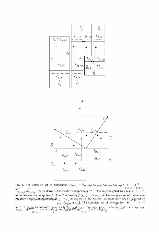
In Fig. 1, we consider a derived-Anosov diffeomorphism g : T → T semi-conjugated, by

a map π : T → T , to the Anosov automorphism f : T → T defined by f (x, y) = (x + y, y), where T = R2 \ (Zv.. × Zw.. ). We exhibit the complete set of holonomies Hf, = {h(A,A), h(A,B), h(B,A), h

−1 −1 −1

(A,A), h(A,B), h(B,A)} associated to the Markov partition M = {A, B}

of f . The derived-Anosov diffeomorphism g admits a Markov partition Mg = {A1, A2, B1} with the property that A = π(A1) ∪ π(A2) and B = π(B1). The complete set of holonomies Hg,Mg

D D

is related to Hf,M as follows: h(A,B) ◦ π |π(£(A1,B1)) = π ◦ h(A1,B1), h(A,A) ◦ π |π(£(A2,A1)) = π ◦ h(A2,A1), h(B,A) ◦ π |π(£D

) = π ◦ h(B ,A ) and h(B,A) ◦ π |π(£D ) = π ◦ h(B ,A ).

(B1,A1) 1 1 (B1,A2) 1 2

Lemma 1. The triple (f, Λ, M) induces a train track Tf with a set of canonical parametriza-

tions. Furthermore, the atlas As (f, ρ) induces a C1+α atlas Bs (f, ρ) in Tf .

1 1 1

Fig. 1. The complete set of holonomies Hg,Mg = {h(A1,B1), h(A2,A1), h(B1,A1), h(B1,A2), h−

, h−1 ,

h−1 −1 (A1,B1) (A2,A1)

(B1,A1), h(B1,A2)} for the derived-Anosov diffeomorphism g : T → T semi-conjugated, by a map π : T → T ,

to the Anosov automorphism f : T → T defined by f (x, y) = (x + y, y). The complete set of holonomies

for the Anosov automorphism f : T → T associated to the Markov partition M = {A, B} is given by Hf,M = {h(A,A), h(A,B), h(B,A), h− − −

g,Mg

(A,A), h(A,B), h(B,A)}. The complete set of holonomies H is re- D D

lated to Hf,M as follows: h(A,B) ◦ π |π(£(A1,B1)) = π ◦ h(A1,B1) , h(A,A) ◦ π |π(£(A2,A1)) = π ◦ h(A2,A1) , h(B,A) ◦ π |π(£D

) = π ◦ h(B ,A ) and h(B,A) ◦ π |π(£D ) = π ◦ h(B ,A ) .

(B1,A1) 1 1 (B1,A2) 1 2

1

Mi

M

(M,N ) N

Proof. For every leaf segment £M ∈ I , let £M be the smallest full leaf segment containing £M

(see definition in Appendix A). Let £M be a full leaf segment that is a small extension of the leaf £M , that compactly contains £M , and does not intersect any other Markov rectangle. By

the Stable Manifold Theorem, there are C1+H diffeomorphisms kM : £M → K M . We choose the

C1+H diffeomorphisms kM : £M → K M with the extra property that their images are pairwise

disjoint, i.e., K M ∩ K N = ∅ for all M, N ∈ M such that M /= N . Set K M = kM (£M ),

n

K M =

K Mi ,

i=1

n

L M =

£Mi ,

i=1

n

L M =

£Mi and LM = L M ∩ Λf . (2)

i=1

Let k : L M → K M be the map defined by k|£M = kM , for every M ∈ M. Let

n

π : Mi → LM (3)

i=1

be the projection defined by π(xi) = yi , where yi ∈ £u (xi ) ∩ LM for every xi ∈ Mi . The end-

points xi ∈ £Mi and xj ∈ £Mj are in the same endpoints equivalence class, if there are points

xi ∈ £Mi and xj ∈ £Mj with the following properties:

(i) k−1

([xi, xi ]) ∩ Λf = k−1(xi );

Mi Mi

(ii) k−1

([xj , xj ]) ∩ Λf = k−1 (xj );

Mj Mj

(iii) There is a closed stable leaf segment £s (yi , yj ) such that

£s (yi , yj ) ∩ Λf = £s (yi , yj ) ∩ f int £u

(k−1

(xi )), int £u

(k−1

(xj )) .

Mi Mi Mj Mj

The endpoints equivalence class in L M is the minimal equivalence class satisfying the above

properties.

For every stable leaf segment £s , consider the smallest full leaf segment £s containing £s and

a chart j : £s → I in the atlas As (f, ρ). By [18], for every Markov rectangle M , the holonomy

h : £s ∩ M → £M has a C1+α extension with respect to the charts in the atlas As (f, ρ), which

implies that the map kM ◦ h ◦ j −1|j (M ∩ £s) has a C1+α diffeomorphic extension uM to the train

track Tf . Therefore, the map π ◦ j −1|(I ∩ j (£s )) has a homeomorphic extension τ : I → Tf such that k

−1 ◦ τ |j (M ∩ £s) = kM ◦ h ◦ j −1 and k−1 ◦ τ = uM is a C1+α diffeomorphism, for

M M

every Markov rectangle M . The inverse of these parametrizations τ together with the previous charts k

−1, for every M ∈ M, forma C1+α atlas Bs (f, ρ) induced by As (f, ρ). ✷

Lemma 2. The triple (f, Λ, M) induces a C1+H Cantor exchange system

Φ = Φf,M = fe(M,N ) : kM

(£(M,N )

) → kN

(£(M,N )

) (M, N) ∈ P

,

D C

with bounded geometry with respect to the atlas Bs (f, ρ) on Tf = Tφ. Furthermore, for every

(M, N) ∈ P, e(M,N )|kM (£D ) = kM ◦ h(M,N ) ◦ k−1

.

(M,N ) N

N |k : k(£

k(£

M

i=1

h(N ,N ) = hα α D

i j n 1 i M αi (Ni ,Nj ) i

k |k(£

D

Proof. Define e(M,N )|kM (£D ) = kM ◦ h(M,N ) ◦ k−1

. By Theorem 2.1 in [18], the map kM ◦

h(M,N ) ◦k−1 M

D (M,N )

) extends (not uniquely) to a C1+α diffeomorphism e (M,N ) (M,N )) →

C (M,N ) ) for some α > 0. By Lemma 1, the set {e(M,N ): (M, N) ∈ P} satisfies properties (i),

(ii) and (iii) of the definition of a C1+H Cantor exchange system. ✷

3. Renormalization of Cantor exchange systems

In this section, given a C1+H diffeomorphism f with codimension 1 hyperbolic attractor Λ and with a Markov partition M satisfying the disjointness property, we present an explicit

construction of a renormalization operator R = Rf,M acting on the topological conjugacy

class of the C1+H Cantor exchange system Φf, induced by (f, Λ, M). Let the Markov

partition N = f∗M be the pushforward of the Markov partition M, i.e., for every M ∈ M,

N = f (M) ∈ N .

Lemma 3. Let Φf,M and Φf,N be the C 1+H

Cantor exchange systems induced (as in Lemma 2),

respectively, by (f, Λ, M) and (f, Λ, N ). There is a well-defined renormalization operator

R = Rf,M : [Φf,M]C0 → [Φf,N ]C0 .

Proof. For simplicity of notation, let us denote kM by k (see (2)). We choose a map

σ : {1,..., n}→ {1,..., n} (4)

with the property that Ni ∩ Mσ(i) /= ∅, where Ni ∈ N and Mσ(i) ∈ M. For each Ni ∈ N , let

£Ni be the stable spanning leaf segment £Mσ (i) ∩ π(Ni ), and let £Ni be the corresponding full n

stable spanning leaf (i.e., £Ni ∩ Λ = £Ni ), where π : /

Mi → LM is the natural projection as defined in (2). Set

LN =

n

i=1

£Ni and

LN =

n

i=1

£Ni .

The set LN determines the train track TN with atlas B(f, ρ) as constructed in Lemma 1. Let D C

HN = {h(Ni ,Nj ) : £(Ni ,Nj ) → £(Ni ,Nj )

|(Ni , Nj ) ∈ PN } be the (stable) primitive holonomic sys-

tem associated to the Markov partition N . By construction, for every (Ni , Nj ) ∈ PN there is a

sequence hα1 , . . . , hαn of holonomies in HM such that

Let

i j n ◦ · · · ◦ h 1 |£Ni .

e(Ni ,Nj ) : kMσ (i)

(£(Ni ,Nj )

) → kMσ (j)

(£(Ni ,Nj )

)

D D

be given by e(N ,N ) = eα ◦ · · · ◦ eα , where eα ∈ Φf, and e |k(£D ) = k ◦ hα ◦ −1 D

(Ni ,Nj ) ). Set

Ψ = fe(N ,N ) : k

(£D

) → k

(£C

) (Ni , Nj ) ∈ P

i j (Ni ,Nj ) (Ni ,Nj ) N

(£

M

N

N

h(M ,M )|£D = θN i j Nj

1

By construction, Ψ = Φf,N (as constructed in Lemma 2), and so Ψ is a C 1+H Cantor exchange

system. Since the set S(Φf,M, Φf,N ) of all sequences α1 . . . αn such that e(Ni ,Nj ) = eαn ◦ · · · ◦ 1+H

eα1 , for some (Ni , Nj ) ∈ PN , form a renormalizable sequence set, the C Cantor exchange

system Φf,N is a renormalization of Φf,M. Therefore, by Section 1.3, there is a well-defined renormalization operator R = Rf,M : [Φf,M]C0 → [Φf,N ]C0 . ✷

Lemma 4. The C1+H Cantor exchange system Φf, is a C1+H fixed point of renormalization,

i.e ., [RΦf,M]C0 = [Φf,M]C0 , where R = Rf,M : [Φf,M]C0 → [Φf,N ]C0 is the renormalization operator (as constructed in Lemma 3).

Proof. We construct a C1+α conjugacy Θ : K → KM between Φ f,M and Φ f,N . For every

N ∈ N and M = f −1(N ), there is a holonomy θN between the spanning leaf segments f −1(£N )

and £M . By Theorem 2.1 in [18], the holonomy θN has a C1+α diffeomorphic extension

θN : f −1(£N ) → £M . Let Θ : K → KM be the C1+α diffeomorphism given by

Θ|k(£N ) = k ◦ θN ◦ f −1 ◦ k−1 (5)

for every N ∈ N . We observe that each pair

(Ni , Nj ) ∈ PN

determines a unique pair (Mi , Mj ) = (f −1(Ni ), f −1(Nj )) ∈ P , and vice versa. Hence, it is D

M D

enough to prove that Θ conjugates φ(Ni ,Nj )|£(Ni ,Nj ) with φ(Mi ,Mj )|£(Mi ,Mj )

, for every (Ni , Nj ) ∈ 1+H

PN , to show that Φf,M is a C fixed point of renormalization.

By construction of the maps θNi and θNj , we have that

i j (Mi ,Mj ) i ◦ f − ◦ h(N ,N ) ◦ f ◦ θ

−1,

and so

1 D −1 −1 −1 −1 −1

Θ ◦ e(Ni ,Nj ) ◦ Θ− |£(Mi ,Mj ) = k ◦ θNj ◦ f ◦ k ◦ k ◦ h(Ni ,Nj ) ◦ k

1

◦ k ◦ f ◦ θNj ◦ k

which ends the proof. ✷

= k ◦ h(Mi ,Mj ) ◦ k−

= e(Mi ,Mj ),

4. Markov maps versus renormalization

The map F : T → T determines a C1+α Markov map, with respect to the atlas B and with invariant set Ω , if the following properties are satisfied:

(i) F : T → T is a local C1+α diffeomorphism with respect to the C1+α atlas B on the train track T.

i=1 i=1

M M

◦

M

Ff, (j −1)

M

(ii) There exist c> 0 and λ> 1 such that, for every x ∈ Ω ,

( ) d jn ◦ Fn ◦ i−1 (x) > cλn, (6)

with respect to charts i, jn ∈ B.

(iii) The map F admits a Markov partition {K1,..., Km}, i.e., there exists a finite set of arcs

{K 1, . . . , K m} such that (a) Ki = K i ∩ Ω , (b) /m

∂K i ⊂ Ω , and (c) F (∂K i ) ⊂ /m

∂K i ,

for every j = 1,..., m.

Let F : L → L be the map induced by the action of f −1

on stable leaf segments, i.e.,

F (x) = π ◦ f −1(x) for every x ∈ L (see (3)). Since f is a local diffeomorphism, the map F

is a local homeomorphism. Let F : kM(LM) → kM(LM) be the map defined by F = kM ◦ F k

−1. Since the holonomies have C1+α extensions (see Theorem 2.1 in [18]), and the map

M

f is C1+α , for some α > 0, the map F has a C1+α extension Ff, : Tf → Tf , with respect to

the atlas Bι(f, ρ), (not uniquely determined) that is a C1+α Markov map with Markov partition

{kM ◦ π(M1),..., kM ◦ π(Ml)}, where M = {M1,..., Ml } is the Markov partition of f (see 1+α

also A. Pinto and D. Rand [19]). Hence, the map Ff,M : Tf → Tf constructed above is a C Markov map. For every j � 1, let L

(j) be the j th level of the partition of Φf, , as presented

0 M (j)

in Section 1.5. By construction, the map Ff,M sends each interval I ∈ L0 onto an interval

M(I ) ∈ L0 , for every j > 0.

Definition 4.1. Let h : ΩΦ → ΩΨ be the topological conjugacy between a C1+H Cantor ex-

change system Ψ = {ψi : Iψi → Jψi ; i = 1, . . ., m} and Φf,M = {φi : Iφi → Jφi ; i = 1,. . ., n}.

We say that Ψ induces a C1+H Markov map

FΨ : TΨ → TΨ ,

if FΨ is a C1+α Markov map, for some α> 0, and FΨ ◦ h(x) = h ◦ Ff,

(x), for every x ∈ ΩΨ .

Lemma 5. Let Φf,M be a C 1+H Cantor exchange system induced by (f, Λ, M).A C 1+H

1+H Can-

tor exchange system Ψ ∈ [Φf,M]C0 , with bounded geometry, determines a C 1+H

Markov map

FΨ topologically conjugate to Ff,M if, and only if, Ψ is a C

tion operator Rf,M.

Remark 2. Lemma 5 also holds for C1,α regularities.

fixed point of the renormaliza-

Proof of Lemma 5. For simplicity of notation, let us denote kM by k (see (2)). Let 1+α

Θ : KN → KM be the C diffeomorphism as constructed in (5). For every N ∈ N , let

M = f −1(N ) ∈ M. Recall that £N ⊂ £M

σ(i) ⊂ LM (see (4)). By construction of F = F f,M

and Θ , the spanning leaf segment £N ⊂ LN has the property that F ◦ k(£N ) = k(£M ) and

F |k(£N ) = Θ . Therefore,

F |KN = Θ. (7)

0

0

1

2 g1

Every leaf segment £ ⊂ LM with the property that F ◦ k(£) = k(£M ) is a spanning leaf segment

of N . Therefore, there is a sequence eα1 , . . . , eαp of Cantor exchange maps in Φ = Φf,M such that

Furthermore,

eαp ◦ · · · ◦ eα1

(k(£)

) = k(£N ).

F |k(£) = Θ ◦ eαp ◦ · · · ◦ eα1 . (8)

FΨ |ξ(KN ) = Θ. (9)

Letting £N , £ and eα1 , . . . , eαp be as above, by (8), we obtain that

FΨ |ξ ◦ k(£) = ΘΨ ◦ eαp ◦ · · · ◦ eα1

. (10)

By (9), if FΨ is C1+α then ΘΨ is C1+α . By (10), if ΘΨ is C1+α then FΨ is C1+α .

Let L(j)

be the j th level of the partition of Ψ (see Section 1.3). By construction, the map FΨ

sends each interval I ∈ L(j)

onto an interval FΨ (I ) ∈ L(j −1)

for every j > 0. Hence, if Ψ has 0 0

bounded geometry we obtain that the length of the sets in L(j)

converge exponentially fast to

0 when j tends to infinity. Therefore, using the Mean Value Theorem, we obtain that if Ψ has

bounded geometry then FΨ satisfies property (ii) and, conversely, if FΨ satisfies property (ii)

we obtain that Ψ has bounded geometry. So, we conclude that if Ψ is a C1+α Cantor exchange system, with bounded geometry, then FΨ is a C1+α Markov map, and vice versa. ✷

5. Proofs of Theorems 1 and 2

Proof of Theorem 1. Let g ∈ F be topologically conjugated to f by a map ug : Uf → Ug , where Uf and Ug are open neighborhoods of Λf and Λg , respectively. The Markov partition M deter-

mines a Markov partition Mg such that, for every M ∈ M, we have that Mg = ug (M) ∈ Mg .

We denote the set ug(L M) by L g . Letting Lg = L g ∩ Λg , we have that Lg = ug (LM). By

the Stable Manifold Theorem, there is a C1+H diffeomorphism kg : L g → Kg with the similar 1+H

properties as the map k : L M → KM . The triple (g, Λg, Mg) induces a C system

Cantor exchange

with bounded geometry. Let g1, g2 ∈ F be C1+H conjugate by a map u : Ug

→ Ug2 , where

Ug1 and Ug2 are open neighborhoods of Λg1 and Λg2 , respectively. By construction, the map

u = kg ◦ u ◦ k−1 is a C 1+H diffeomorphism, and

−

g

g

1

Mg

Therefore, u is a C1+H conjugacy between Φg , Mg and Φg , Mg , and so the map Tf, is

well defined. 1 1 1 1 M

Proof of statement (a). Since the holonomies are C1+α (see A. Pinto and D. Rand [18]), the

Hausdorff dimension of the stable leaf segments £ is the same independently of the stable leaf

segment considered, and so equal to HD(Λs ). In particular, all leaf segments £Mg ∈ Ig have the same Hausdorff dimension which is equal to the Hausdorff dimension of Lg . Since the Can-

tor invariant set TΦg,Mg is equal to k(Lg), the Hausdorff dimension HD(TΦg,Mg

) is equal to

HD(Λs ).

Proof of statement (b). By Lemma 4, if g ∈ F , then the C1+H Cantor exchange system Φg,

is a fixed point of the renormalization operator Rg,Mg that, by construction, is the same as Rf,M.

Hence, T (F) ⊂ CR .

The proof that T (F) ⊃ CR follows from the proof of the statement (c) below.

Proof of statement (c). Let Φ be a C1+H Cantor exchange system such that [RΦ]C1+H = [Φ]C1+H . Since [RΦ]C1+H = [Φ]C1+H , by Lemma 5, the C1+H Cantor exchange system Φ in- duces a Markov map FΦ . Therefore, (Φ, FΦ) is a self-renormalizable structure as defined in [15] and [16]. By Theorem 1.14 in [15] (see also A. Pinto and D. Rand [16]), there is a one-to-one

correspondence between C1+H conjugacy classes of (Φ, FΦ) and C1+H conjugacy classes of

C1+H diffeomorphisms g(Φ, FΦ) with hyperbolic invariant set Λg , and with an invariant mea- sure absolutely continuous with respect to the Hausdorff measure.

Proof of statement (d). Let Φ be a C1+H Cantor exchange system such that [RΦ]C1+H =

[Φ]C1+H . Since [RΦ]C1+H = [Φ]C1+H , by Lemma 5, the C1+H Cantor exchange system Φ in-

duces a Markov map FΦ . Let CF be the set of all C1+H conjugacy classes of pairs (Φ, FΦ).

Hence, there is a one-to-one map m1 : CR → CF given by m1(Φ) = (Φ, FΦ). By Lemma 4.2 in [15] (see also A. Pinto and D. Rand [16]), there is a well-defined Teichmüller space TS con-

sisting of solenoid functions, and a one-to-one map m2 : TS → CF given by m2(s) = (Φ, FΦ). Therefore, m

−1 ◦ m2 : TS → CR is a one-to-one map. ✷

Proof. By Theorem 1.14 in [15], given a C1+α Cantor exchange system Ψ and a C1+α Markov

map FΨ , there is a C1+α diffeomorphism with a codimension 1 hyperbolic attractor set with

an invariant measure absolutely continuous with respect to the Hausdorff measure, topologically

conjugate to f which induces Ψ . Hence, by Lemma 5, Ψ is a C1+β fixed point of renormaliza- tion, for some β > 0, which implies Lemma 6. ✷

Proof of Theorem 2. Let us suppose that the Cantor exchange system Ψ is a C1,α fixed point

of the renormalization operator Rf,M with α = HD(TΨ ) and with bounded geometry. Hence,

by Lemma 5, Ψ induces a C1,α Markov map FΨ . Let ξ be the homeomorphic extension of the

n;?1

0

(M,N ) → £

(M,N )

0

conjugacy between Φ and Ψ , and set η = ξ ◦ k ◦ π . Let Tn be the set of all pairs (I, J ) such that (i) I is a stable leaf n-cylinder, (ii) J is a stable leaf n-cylinder or a stable n-gap cylinder, and (iii) I and J have a unique common endpoint (see Appendix A.4). Using the Mean Value

Theorem and that FΨ is a C1,α Markov map, the function r : /

Tn → R+ given by

r(I, J ) =

m lim |η ◦ f m(J )|

→+∞ |η ◦ f m(I )|

is well defined, where |L| means the length of the smallest interval containing L ⊂ R. By bounded geometry of Ψ , we obtain that r is bounded away from zero. Furthermore, using that

FΨ is a C1,α Markov map, for every pair (I, J ) ∈ Tn, we get

where Cn ∈ R+ converges to zero when n tends to infinity.

Let h = h(M,N ) : £D

C (M,N )

be a ι-primitive holonomy. Since the Cantor exchange

system is C1,α , for every (I, J ) ∈ Tn such that I ∪ J ⊂ £D , we get

α

where Cn ∈ R+ converges to zero when n tends to infinity.

From (11), we obtain that

Thus, using (12) we get

where C 1 ∈ R+

converges to zero when n tends to infinity. n 0

Since α = HD(TΨ ), by the Rigidity Lemma 4.1 in [17], we obtain that r is a stable trans- versely affine ratio function (see definition in Appendix A.7). However, putting together Theo-

rem 1 and Lemma 1 in [22], there are no stable transversely affine ratio functions with respect to the stable lamination of Λf , and so we get a contradiction. ✷

Acknowledgments

We are very grateful to Welington de Melo and Stefano Luzzatto for very useful discussions on

this work. We thank the referee for his useful comments. We thank IHES, CUNY, IMPA, Stony

Brook and University of Warwick for their hospitality. We thank Calouste Gulbenkian Founda-

tion, PRODYN-ESF, POCTI and POCI by FCT and Ministério da Ciência e da Tecnologia and

Centros de Matemática da Universidade do Minho e da Universidade do Porto for their financial

support of A.A. Pinto and F. Ferreira, and the Wolfson Foundation and the UK Engineering and

Physical Sciences Research Council for their financial support of D.A. Rand.

Appendix A

In this appendix, we present some basic facts for C1+H hyperbolic diffeomorphisms (f, Λ),

that we include for clarity of the exposition. We say that (f, Λ) is a C1+H hyperbolic diffeomor-

phism, if (f, Λ) has the following properties:

(i) f : S → S is a C1+α diffeomorphism of a compact surface S with respect to a C1+α structure on S, for some α> 0.

(ii) Λ is a hyperbolic invariant subset of S such that f |Λ is topologically transitive and Λ has a local product structure.

In particular, a C1+H diffeomorphism f with a codimension 1 attractor Λ is a C1+H hyperbolic

diffeomorphism.

A.1. Leaf segments

Let d bea metric on M , and define the map fι = f if ι = u, or fι = f −1 if ι = s. For ι ∈ {s, u},

if x ∈ Λ we denote the local ι-manifolds through x by

By the Stable Manifold Theorem (see [9] and [25]), these sets are respectively contained in the

stable and unstable immersed manifolds

which are the image of a C1+γ immersion κι,x : R → M . An open (respectively closed) full ι-leaf

segment I is defined as a subset of Wι(x) of the form κι,x (I1) where I1 is an open (respectively closed) subinterval (non-empty) in R. An ι-open (respectively closed) leaf segment is the in-

tersection with Λ of a full open (respectively closed) ι-leaf segment such that the intersection

contains at least two distinct points. If the intersection is exactly two points we call this ι-closed

leaf segment an ι-leaf gap. An ι-full leaf segment is either an open or closed ι-full leaf segment.

An ι-leaf segment is either an open or closed ι-leaf segment. The endpoints of a full ι-leaf seg-

ment are the points κι,x (u) and κι,x (v) where u and v are the endpoints of I1. The endpoints of

an ι-leaf segment I are the points of the minimal closed full ι-leaf segment containing I . The

interior of a ι-leaf segment I is the complement of its boundary. In particular, a ι-leaf segment

I has empty interior if, and only if, it is an ι-leaf gap. A map c : I → R is an ι-leaf chart of an

ι-leaf segment I if has an extension cE : IE → R to a full ι-leaf segment IE with the following

properties: I ⊂ IE and cE is a homeomorphism onto its image. An ι-full leaf segment is either an open or close full leaf segment.

i=1

A.2. Rectangles

Since Λ is a hyperbolic invariant set of a diffeomorphism f : M → M , for 0 <ε < ε0 there

is δ = δ(ε) > 0, such that for all points w, z ∈ Λ with d(w, z) < δ, Wu(w, ε) and Ws (z, ε)

intersect in an unique point that we denote by [w, z]. Since we assume that the hyperbolic set

has a local product structure, we have that [w, z]∈ Λ. Furthermore, the following properties

are satisfied: (i) [w, z] varies continuously with w, z ∈ Λ; (ii) the bracket map is continuous on

a δ-uniform neighborhood of the diagonal in Λ × Λ; and (iii) whenever both sides are defined

f ([z, w]) = [f (z), f (w)]. Note that the bracket map does not really depend on δ provided it is sufficiently small.

Let us underline that it is a standing hypothesis that all the hyperbolic sets considered here

have such a local product structure.

A rectangle R is a subset of Λ which is (i) closed under the bracket, i.e., x, y ∈ R ⇒ [x, y]∈ R, and (ii) proper, i.e., is the closure of its interior in Λ. This definition imposes that a rectangle

has always to be proper which is more restrictive than the usual one which only insists on the

closure condition. If £s and £u are respectively stable and unstable leaf segments intersecting in a single

point then we denote by [£s , £u] the set consisting of all points of the form [w, z] with

w ∈ £s and z ∈ £u. We note that if the stable and unstable leaf segments £ and £1 are closed

then the set [£, £1] is a rectangle. Conversely in this 2-dimensional situations, any rectan- gle R has a product structure in the following sense: for each x ∈ R there are closed sta-

ble and unstable leaf segments of Λ, £s (x, R) ⊂ W s (x) and £u(x, R) ⊂ W u(x) such that

R = [£s (x, R), £u(x, R)]. The leaf segments £s (x, R) and £u(x, R) are called stable and un-

stable spanning leaf segments for R. For ι ∈ {s, u}, we denote by ∂ £ι(x, R) the set consisting

of the endpoints of £ι(x, R), and we denote by int £ι(x, R) the set £ι(x, R) \ ∂ £ι(x, R). The in-

terior of R is given by int R = [int £s (x, R), int £u(x, R)], and the boundary of R is given by

∂R = [∂ £s (x, R), £u(x, R)] ∪ [£s (x, R), ∂ £u(x, R)].

A.3. Markov partitions

By Theorem 3.12 in page 79 of [2] (see also Sinai [26]), a Markov partition of f is a collection

R = {R1, . . . , Rk } of such rectangles such that (i) Λ ⊂ /k

Ri ; (ii) Ri ∩ Rj = ∂Ri ∩ ∂Rj for

all i and j ; (iii) if x ∈ int Ri and fx ∈ int Rj then

(a) f (£s (x, Ri )) ⊂ £s (f x, Rj ) and f −1(£u(f x, Rj )) ⊂ £u(x, Ri );

(b) f (£u(x, Ri )) ∩ Rj = £u(f x, Rj ) and f −1(£s (f x, Rj )) ∩ Ri = £s (x, Ri ).

The last condition means that f (Ri ) goes across Rj just once. In fact, it follows from condi-

tion (a) providing the rectangles Rj are chosen sufficiently small (see Mañé [10]). The rectangles

which make up the Markov partition are called Markov rectangles.

We note that there is a Markov partition R of f with the following disjointness property (see

R. Bowen [2], S. Newhouse and J. Palis [12], Ya. Sinai [26]):

(i) If 0 < δf,s < 1 and 0 < δf,u < 1 then the stable and unstable leaf boundaries of any two

Markov rectangles do not intersect.

(ii) If 0 < δf,ι < 1 and 0 < δf,ι1 = 1 then the ι1-leaf boundaries of any two Markov rectangles do not intersect except, possibly, at their endpoints.

If δf,s = δf,u = 1, the disjointness property does not apply and so we consider that it is trivially

satisfied for every Markov partition. For simplicity of our exposition, we consider Markov parti- tions that satisfy the disjointness property. This result is also used in [5–7,20,21,23] and [24].

A.4.

A.5. Basic holonomies

Suppose that x and z are two points inside any rectangle R of Λ. Let I and J be two stable

leaf segments respectively containing x and z and inside R. Then we define h : I → J by h(w) =

[w, z]. Such maps are called the basic stable holonomies. They generate the pseudo-group of all stable holonomies. Similarly we define the basic unstable holonomies.

A.6. Conjugacies

Let (f, Λ) be a C1+H hyperbolic diffeomorphism. Somewhat unusually we also desire to

highlight the C1+H structure on M in which f is a diffeomorphism. By a C1+H structure on M

we mean a maximal set of charts with open domains in M such that the union of their domains

cover M and whenever U is an open subset contained in the domains of any two of these charts

i and j then the overlap map j ◦ i−1 : i(U) → j (U ) is C1+α , where α > 0 depends on i, j

and U . We note that by compactness of M , given such a C1+H structure on M , there is an atlas

consisting of a finite set of these charts which cover M and for which the overlap maps are C1+α

compatible and uniformly bounded in the C1+α norm, where α > 0 just depends upon the atlas.

We denote by Cf the C1+H structure on M in which f is a diffeomorphism. Usually one is not

concerned with this as, given two such structures, there is a homeomorphism of M sending one

onto the other and thus, from this point of view, all such structures can be identified. For our

discussion it will be important to maintain the identity of the different smooth structures on M .

We say that a map h : Λf → Λg is a topological conjugacy between two C1+H hyperbolic

diffeomorphisms (f, Λf ) and (g, Λg) if there is a homeomorphism h : Λf → Λg with the fol- lowing properties:

(i) g ◦ h(x) = h ◦ f (x) for every x ∈ Λf .

(ii) The pull-back of the ι-leaf segments of g by h are ι-leaf segments of f .

ι1

Definition 6.1. Let F be the set of all C1+H hyperbolic diffeomorphisms (g, Λg) such that

(g, Λg) and (f, Λ) are topologically conjugate by h.

A.7. HR-Hölder ratios

A HR-structure associates an affine structure to each stable and unstable leaf segment in such

a way that these vary Hölder continuously with the leaf and are invariant under f .

An affine structure on a stable or unstable leaf is equivalent to a ratio function r(I : J) which can be thought of as prescribing the ratio of the size of two leaf segments I and J in the same

stable or unstable leaf. A ratio function r(I : J) is positive (we recall that each leaf segment has at least two distinct points) and continuous in the endpoints of I and J . Moreover,

r(I : J) = r(J : I )−1 and r(I1 ∪ I2 : K) = r(I1 : K) + r(I2 : K) (13)

provided I1 and I2 intersect at most in one of their endpoints.

We say that r is a ι-ratio function if (i) for all ι-leaf segments K , r(I : J) (I, J ⊂ K ) defines a

ratio function on K ; (ii) r is invariant under f , i.e., r(I : J) = r(f I : fJ) for all ι-leaf segments;

and (iii) for every basic ι-holonomy map θ : I → J between the leaf segment I and the leaf

segment J defined with respect to a rectangle R and for every ι-leaf segment I0 ⊂ I and every

ι-leaf segment or gap I1 ⊂ I ,

where ∈ (0, 1) depends upon r and the constant of proportionality also depends upon R, but not on the segments considered. Since r satisfies the condition (14) and defines an affine structure on each leaf that is f -invariant we say that r is a transversely Hölder ι-ratio function. A HR-structure

is a pair (rs , ru) consisting of a stable and an unstable ratio function.

Definition 6.2. If an ι-ratio function r is invariant under holonomies h (i.e., r(I : J) = r(h(I) : h(J ))), then we say that r is a transversely affine ι-ratio function.

A.8. Realized ratio functions

Let g ∈ F and ρ = ρg be a C1+ Riemannian metric on the manifold containing Λ. The ι-

lamination atlas Aι(g, ρ) determined by ρ is the set of all maps e : I → R where I = Λ ∩ I

with I a full ι-leaf segment, such that e extends to an isometry between the induced Riemannian

metric on I and the Euclidean metric on the reals. We call the maps e ∈ Aι(g, ρ) the ι-lamination

charts. If I is an ι-leaf segment (or a full ι-leaf segment) then by |I | = |I |ρ we mean the length in the Riemannian metric ρ of the minimal full ι-leaf containing I . By hyperbolicity of g in Λ, there

are 0 <ν < 1 and C > 0 such that for all ι-leaf segments I and all m � 0 we get |gmI | � Cνm|I |. Thus, using the mean value theorem and the fact that gι is Cr , for all short leaf segments K and all leaf segments I and J contained in it, the ι-realized ratio function rg,ι given by

2

ι1

is well defined, where α = min{1,r − 1}. This construction gives the HR-structure on Λ deter- mined by g. By [19], we get the following equivalence:

Theorem 3. The map g → (rg,s , rg,u) determines a one-to-one correspondence between C1+H

conjugacy classes in F and HR-structures.

A.9. Lamination atlas

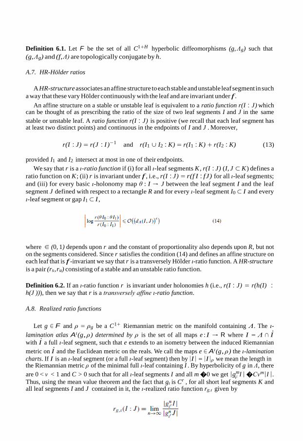
Given an ι-ratio function r , we define the embeddings e : I → R by

where ξ is an endpoint of the ι-leaf segment I and R is a Markov rectangle containing ξ (see

Fig. 2). For this definition it is not necessary that R contains I . We denote the set of all these

embeddings e by A(r).

Let g ∈ F and A(g, ρ) the ι-lamination atlas determined by a Riemannian metric ρ. Putting

together Propositions 2.5 and 3.5 of [19], we get that the overlap map e1 ◦ e−1 between a chart has a C1+H diffeomorphic extension to the reals. Therefore,

e1 ∈ A(g, ρ) and a chart e2 ∈ A(rg,ι) for all short leaf segments K and all leaf segments I and J contained in it, we obtain that

where in is any chart in A(rg,ι) containing the segment gnK in its domain.

A.10. Realized solenoid functions

For ι = s and u, let Sι denote the set of all ordered pairs (I, J ) of ι-leaf segments with the following properties:

Fig. 2. The embedding e : I → R.

(i) The intersection of I and J consists of a single endpoint.

(ii) If δf,ι = 1 then I and J are primary ι-leaf cylinders.

(iii) If 0 < δf,ι < 1 then fι1 I is an ι-leaf 2-cylinder of a Markov rectangle R and fι1 J is an ι-leaf

2-gap also of the same Markov rectangle R.

See Appendix A.4 for the definitions of leaf cylinders and gaps. Pairs (I, J ) where both are primary cylinders are called leaf-leaf pairs. Pairs (I, J ) where J is a gap are called leaf-gap

pairs and in this case we refer to J as a primary gap. The set Sι has a very nice topological

structure. If δf,ι1 = 1 then the set Sι is isomorphic to a finite union of intervals, and if δf,ι1 < 1 then the set Sι is isomorphic to an embedded Cantor set.

We define a pseudo-metric dSι : Sι × Sι → R+ on the set Sι by

.

Let g ∈ T (f, Λ). For ι = s and u, we call the restriction of an ι-ratio function rg,ι to Si a realized

solenoid function σg,ι. By construction, for ι = s and u, the restriction of an ι-ratio function to Si

gives an Hölder continuous function satisfying the matching condition, the boundary condition

and the cylinder-gap condition as we now proceed to describe.

A.11. Hölder continuity of solenoid functions

This means that for t = (I, J ) and t 1 = (I 1, J 1) in Sι , |σι(t ) − σι(t 1)| � O((dSι (t, t 1))α ). The Hölder continuity of σg,ι and the compactness of its domain imply that σg,ι is bounded away from zero and infinity.

A.12. Matching condition

Let (I, J ) ∈ Sι be a pair of primary cylinders and suppose that we have pairs

Fig. 3. The f -matching condition for ι-leaf segments.

Hence, noting that g|Λ = f |Λ, the realized solenoid function σg,ι must satisfy the matching condition (see Fig. 3) for all such leaf segments:

.

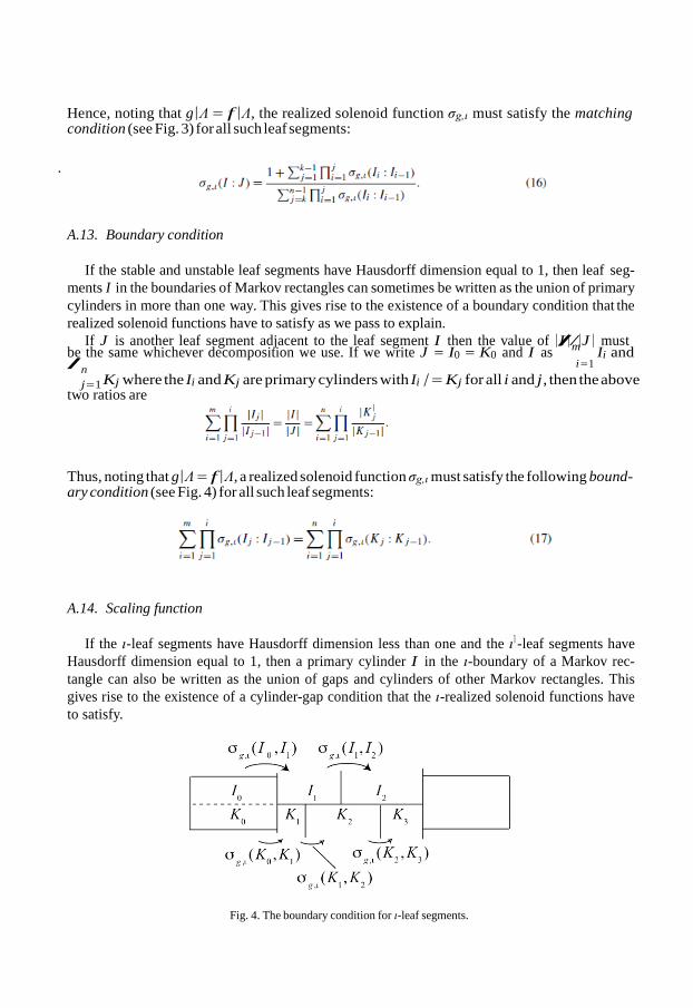
A.13. Boundary condition

If the stable and unstable leaf segments have Hausdorff dimension equal to 1, then leaf seg-

ments I in the boundaries of Markov rectangles can sometimes be written as the union of primary

cylinders in more than one way. This gives rise to the existence of a boundary condition that the

realized solenoid functions have to satisfy as we pass to explain.

If J is another leaf segment adjacent to the leaf segment I then the value of |I |/|J | must be the same whichever decomposition we use. If we write J = I0 = K0 and I as

/m Ii and

/n i=1

j =1 Kj where the Ii and Kj are primary cylinders with Ii /= Kj for all i and j , then the above two ratios are

Thus, noting that g|Λ = f |Λ, a realized solenoid function σg,ι must satisfy the following bound- ary condition (see Fig. 4) for all such leaf segments:

A.14. Scaling function

If the ι-leaf segments have Hausdorff dimension less than one and the ι1-leaf segments have

Hausdorff dimension equal to 1, then a primary cylinder I in the ι-boundary of a Markov rec-

tangle can also be written as the union of gaps and cylinders of other Markov rectangles. This

gives rise to the existence of a cylinder-gap condition that the ι-realized solenoid functions have

to satisfy.

Fig. 4. The boundary condition for ι-leaf segments.

ι1 ι1

ι1

Before defining the cylinder-gap condition, we will introduce the scaling function that will be

useful to express the cylinder-gap condition.

Let sclι be the set of all pairs (K, J ) of ι-leaf segments with the following properties:

(i) K is a leaf n1-cylinder or an n1-gap segment for some n1 > 1; (ii) J is a leaf n2-cylinder or an n2-gap segment for some n2 > 1;

(iii) mn1−1K and mn2−1J are the same primary cylinder.

Lemma 7. Every function σι : Sι → R+ has a canonical extension sι to sclι. Furthermore, if σι is

the restriction of a ratio function rι|Sι to Sι then sι = rι|sclι.

See proof of Lemma 7 in [15].

Remark 3. The above map sι : sclι → R+ is the scaling function determined by the solenoid

function σι : Sι → R+.

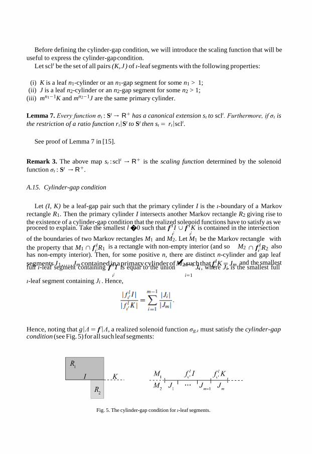
A.15. Cylinder-gap condition

Let (I, K) be a leaf-gap pair such that the primary cylinder I is the ι-boundary of a Markov

rectangle R1. Then the primary cylinder I intersects another Markov rectangle R2 giving rise to

the existence of a cylinder-gap condition that the realized solenoid functions have to satisfy as we proceed to explain. Take the smallest l � 0 such that f l I ∪ f l K is contained in the intersection

ι1 ι1

of the boundaries of two Markov rectangles M1 and M2. Let M1 be the Markov rectangle with

the property that M1 ∩ f l R1 is a rectangle with non-empty interior (and so M2 ∩ f l R2 also

has non-empty interior). Then, for some positive n, there are distinct n-cylinder and gap leaf

segments J1,..., Jm contained in a primary cylinder of M2 such that f l K = Jm and the smallest full ι-leaf segment containing f l I is equal to the union

/m−1 Ji , where Ji is the smallest full

ι1

ι-leaf segment containing Ji . Hence, i=1

ˆ ˆ

Hence, noting that g|Λ = f |Λ, a realized solenoid function σg,ι must satisfy the cylinder-gap condition (see Fig. 5) for all such leaf segments:

Fig. 5. The cylinder-gap condition for ι-leaf segments.

where sg,ι is the scaling function determined by the solenoid function σg,ι.

A.16. Solenoid functions

Now, we are ready to present the definition of an ι-solenoid function.

Definition 1. An Hölder continuous function σι : Sι → R+ is an ι-solenoid function if σι satisfies the matching condition, the boundary condition and the cylinder-gap condition.

We denote by PS(f ) the set of pairs (σs , σu) of stable and unstable solenoid functions.

Remark 4. Let σι : Sι → R+ be an ι-solenoid function. The matching, the boundary and the cylinder-gap conditions are trivially satisfied except in the following cases:

(i) The matching condition if δf,ι = 1.

(ii) The boundary condition if δf,s = δf,u = 1.

(iii) The cylinder-gap condition if δf,ι < 1 and δf,ι1 = 1.

Theorem 4. The map rι → rι|Sι gives a one-to-one correspondence between ι-ratio functions and ι-solenoid functions.

See proof of Theorem 4 in [15].

The set PS(f ) of all pairs (σs , σu) has a natural metric. Combining Theorem 3 with Theo-

rem 4, we obtain that the set PS(f ) forms a moduli space for the C1+H conjugacy classes of

C1+H hyperbolic diffeomorphisms g ∈ T (f, Λ):

Corollary 1. The map g → (rg,s |Ss, rg,u|Su) determines a one-to-one correspondence between

C1+H conjugacy classes of g ∈ T (f, Λ) and pairs of solenoid functions in PS(f ).

References

[1] C. Bonatti, R. Langevin, Difféomorphismes de Smale des surfaces, Astérisque 250 (1998).

[2] R. Bowen, Equilibrium States and the Ergodic Theory of Anosov Diffeomorphisms, Lecture Notes in Math.,

vol. 470, Springer-Verlag, New York, 1975.

[3] E. Cawley, The Teichmüller space of an Anosov diffeomorphism of T 2 , Invent. Math. 112 (1993) 351–376.

[4] A. Denjoy, Sur les courbes définies par les équations différentielles à la surface du tore, J. Math. Pures Appl. 11 (9)

(1932) 333–375.

[5] E. de Faria, W. de Melo, A.A. Pinto, Global hyperbolicity of renormalization for Cr unimodal mappings, Ann. of

Math. 164 (2006) 731–824.

[6] F. Ferreira, A.A. Pinto, Explosion of smoothness from a point to everywhere for conjugacies between diffeomor-

phisms on surfaces, Ergodic Theory Dynam. Systems 23 (2003) 509–517.

[7] F. Ferreira, A.A. Pinto, Explosion of smoothness from a point to everywhere for conjugacies between Markov

families, Dyn. Syst. 16 (2) (2001) 193–212.

[8] J. Harrison, An introduction to fractals, in: Proc. Sympos. Appl. Math., vol. 39, Amer. Math. Soc., 1989, pp. 107–

126.

[9] M. Hirsch, C. Pugh, Stable manifolds and hyperbolic sets, in: Proc. Sympos. Pure Math., vol. 14, Amer. Math. Soc.,

1970, pp. 133–164.

[10] R. Mañé, Ergodic Theory and Differentiable Dynamics, Springer-Verlag, Berlin, 1987.

[11] H. Masur, Interval exchange transformations and measured foliations, Ann. of Math. (2) 115 (1) (1982) 169–200.

[12] S. Newhouse, J. Palis, Hyperbolic nonwandering sets on two-dimension manifolds, in: M. Peixoto (Ed.), Dynamical

Systems, Academic Press, New York, 1973, pp. 293–301.

[13] A. Norton, Denjoy’s Theorem with exponents, Proc. Amer. Math. Soc. 127 (10) (1999) 3111–3118.

[14] R.C. Penner, J.L. Harer, Combinatorics of Train Tracks, Princeton University Press, Princeton, NJ, 1992.

[15] A.A. Pinto, D.A. Rand, Geometric measures for hyperbolic sets on surfaces, Stony Brook IMS Preprint 3 (2006)

1–69.

[16] A.A. Pinto, D.A. Rand, Solenoid functions for hyperbolic sets on surfaces, in: Boris Hasselblatt (Ed.), Dynamics,

Ergodic Theory and Geometry: Dedicated to Anatole Katok, Math. Sci. Res. Inst. Publ. 54 (2007) 145–178.

[17] A.A. Pinto, D.A. Rand, Rigidity of hyperbolic sets surfaces, J. London Math. Soc. 71 (2) (2004) 481–502.

[18] A.A. Pinto, D.A. Rand, Smoothness of holonomies for codimension 1 hyperbolic dynamics, Bull. London Math.

Soc. 34 (2002) 341–352.

[19] A.A. Pinto, D.A. Rand, Teichmüller spaces and HR structures for hyperbolic surface dynamics, Ergodic Theory

Dynam. Systems 22 (2002) 1905–1931.

[20] A.A. Pinto, D.A. Rand, Classifying C1+ structures on hyperbolical fractals: 1. The moduli space of solenoid func-

tions for Markov maps on train-tracks, Ergodic Theory Dynam. Systems 15 (1995) 697–734.

[21] A.A. Pinto, D.A. Rand, Classifying C1+ structures on hyperbolical fractals: 2. Embedded trees, Ergodic Theory

Dynam. Systems 15 (1995) 969–992.

[22] A.A. Pinto, D.A. Rand, F. Ferreira, Hausdorff dimension bounds for smoothness of holonomies for codimension 1

hyperbolic dynamics, J. Differential Equations (2007), doi: 10.1016/j.jde.2007.02.013, in press, 11 pp.

[23] A.A. Pinto, D.A. Rand, F. Ferreira, Fine Structures of Hyperbolic Diffeomorphisms, Monograph, Springer-Verlag,

2008.

[24] A.A. Pinto, D. Sullivan, The circle and the solenoid. Dedicated to Anatole Katok on the Occasion of his 60th

Birthday, Discrete Contin. Dyn. Syst. A 16 (2) (2006) 463–504.

[25] M. Schub, Global Stability of Dynamical Systems, Springer-Verlag, 1987.

[26] Ya. Sinai, Markov partitions and C-diffeomorphisms, Anal. Appl. 2 (1968) 70–80.

[27] W. Thurston, On the geometry and dynamics of diffeomorphisms of surfaces, Bull. Amer. Math. Soc. 19 (1988)

417–431.

[28] W. Thurston, The Geometry and Topology of Three-Manifolds, Princeton University Press, Princeton, 1978.

[29] W. Veech, Gauss measures for transformations on the space of interval exchange maps, Ann. of Math. (2) 115 (2)

(1982) 201–242.

[30] R.F. Williams, Expanding attractors, Publ. Math. Inst. Hautes Études Sci. 43 (1974) 169–203.