FORMULATION AND ANALYSIS OF ALTERNATING EVOLUTION (AE) SCHEMES
Chapter 4
Variational Formulation ofBoundary Value Problems
4.1 Elements of Function Spaces
4.1.1 Space of Continuous Functions
• N is a set of non-negative integers.
• 1) An n-tuple ! = (!1, · · · , !n) ! Nn is called a multi-index.
2) The length of ! is
|!| :=n!
j=1
!j.
3) 0¯
= (0, · · · , 0).
• Set D! := ("/"x1)!1 · · · ("/"xn)!n .
Example 4.1.1. Assume n = 3, ! = (!1, !2, !3) ! N3, u(x1, x2, x3) : R3 " R.
29
What is"
|!|=3 D!u ?
|!| = 3 =#3!
j=1
!j = 3.
=# ! = (3,0,0), (0,3,0), (0,0,3), (2,1,0), (2,0,1), (0,2,1),(1, 2, 0), (1, 0, 2), (0, 1, 2), (1, 1, 1).
=#!
|!|=3
D!u ="3u
"x31
+"3u
"x32
+"3u
"x33
+"3u
"x21"x2
+"3u
"x21"x3
+"3u
"x22"x3
+"3u
"x1"x22
+"3u
"x1"x23
+"3u
"x2"x23
+"3u
"x1"x2"x3.
This sort of list can get very long. Hence D! is useful notation.
Definition 4.1.2. Let ! be an open set in Rn. Let k ! N. Define spaces Ck(!),Ck(!) and C!(!) by
Ck(!) := {u : ! " R | D!u is continuous in ! for all |!| $ k},Ck(!) := {u : ! " R | D!u is continuous in ! for all |!| $ k},
C!(!) := {u : ! " R | D!u is continuous in ! for all ! ! Nn},
where ! is the closure of !. If ! is bounded, ! =! %"!, where "! is the boundaryof !. We denote C(!) = C0(!) and C(!) = C0(!).
Example 4.1.3. Set I := (0, 1) and u(x) := 1/x2 &x ! I. Then clearly for allk ' 0 u ! Ck(I). However, in I = [0, 1] u is not continuous at 0. Thus, u /! C(I).
Definition 4.1.4. For a bounded open set ! ( Rn, k ! N and u ! Ck(!), thenorm )u)Ck(!) is defined by
)u)Ck(!) :=!
|!|"k
supx#!
|D!u(x)|.
Example 4.1.5. Let I = (0, 1), u(x) := x, u ! C(I). Then, supx#I |u(x)| = 1.
Definition 4.1.6. For an open set ! ( Rn and u ! C(!) the support of u denotedby supportu (( Rn) is defined by
supportu := the closure of {x ! ! | u(x) *= 0}.
Remark. The support of u is the smallest closed subset of ! such that u = 0 in!\supportu.
30
Example 4.1.7. 1) Let 0 = x0 < x1 < · · · < xn = 1 be a patition of [0, 1]. Define#j(x) : [0, 1] " R by
#j(x) :=
#$$%
$$&
x+ xj$1
hx ! (xj$1, xj),
xj+1 + x
hx ! (xj , xj+1),
0 elsewhere.
Then we see #j ! C(I) and support#j = [xj$1, xj+1].
2) Define w(x) : Rn " R by
w(x) :=
#%
& e$
11+ |x|2 |x| < 1,
0 otherwise.
Then we see w ! C!(Rn) and supportw = {x ! Rn | |x| $ 1}.
Definition 4.1.8. Define Ck0 (!) (( Ck(!)) by
Ck0 (!) := {u ! Ck(!) | supportu is a bounded subset of !}.
4.1.2 Spaces of Integrable Functions
Definition 4.1.9. Let ! denote an open subset of Rn and assume 1 $ p < ,. Wedefine a space of integrable functions Lp(!) by
Lp(!) :='
v : ! " R |(
!|v(x)|pdx < +,
).
The space Lp(!) is a Banach space with norm ) ·) Lp(!) defined by
)v)Lp(!) =*(
!|v(x)|pdx
+1/p
.
Especially the space L2(!) is a Hilbert space with inner product -·, ·.L2(!) definedby
-u, v.L2(!) :=(
!u(x)v(x)dx
and norm ) ·) L2(!) defined by )u)L2(!) :=,-u, v.L2(!).
31
We have Minkowski’s inequality as follows. For u, v ! Lp(!), 1 $ p < ,
)u + v)Lp(!) $ )u)Lp(!) + )v)Lp(!).
We also have Holder’s inequality. For u ! Lp(!) and v ! Lq(!), 1 $ p, q < , with1/p + 1/q = 1
--(
!u(x)v(x)dx
-- $ )u)Lp(!))v)Lq(!).
Now, any two integrable functions are equal if they are equal almost everywhere,that is, they are equal except on a set of zero measure. Strictly speaking, Lp(!)consists of equivalent classes of functions.
Example 4.1.10. Let u, v : (+1, 1) " R be
u(x) ='
1 x ! (0, 1),0 x ! (+1, 0], v(x) =
'1 x ! [0, 1),0 x ! (+1, 0),
The functions u and v are equal almost everywhere, since the set {0} where u(0) *=v(0) has zero measure in the interval (+1, 1). So u and v are equal as integrablefunctions in (+1, 1).
Suppose that u ! Ck(!), where ! is an open set of Rn. Let v ! C!0 (!). Then we
see by integration by parts(
!D!u(x)v(x)dx = (+1)|!|
(
!u(x)D!v(x)dx,
where |!| $ k.
Definition 4.1.11. A function u : ! " R is locally integrable if u ! L1(U) forevery bounded open set U such that U ( !.
Definition 4.1.12. Suppose u : ! " R is locally integrable and there is a locallyintegrable function w! : ! " R such that
(
!w!(x)#(x)dx = (+1)|!|
(
!u(x)D!#(x)dx
for all # ! C!0 (!).
Then the weak derivative of u of order ! denoted by D!u is defined by D!u = w!.
32
Note that at most only one w! satisfies (4.1.12) so the weak derivative of u is well-defined. Indeed, the following DuBois-Raymond lemma shows such w! is unique.
Lemma 4.1.13. (DuBois-Raymond) Suppose ! is an open set in Rn and w : ! " Ris locally integrable. If (
!w(x)#(x)dx = 0
for all # ! C!0 (!), then w(x) = 0 for a.e x ! !.
We will useD for both classical and weak derivatives.
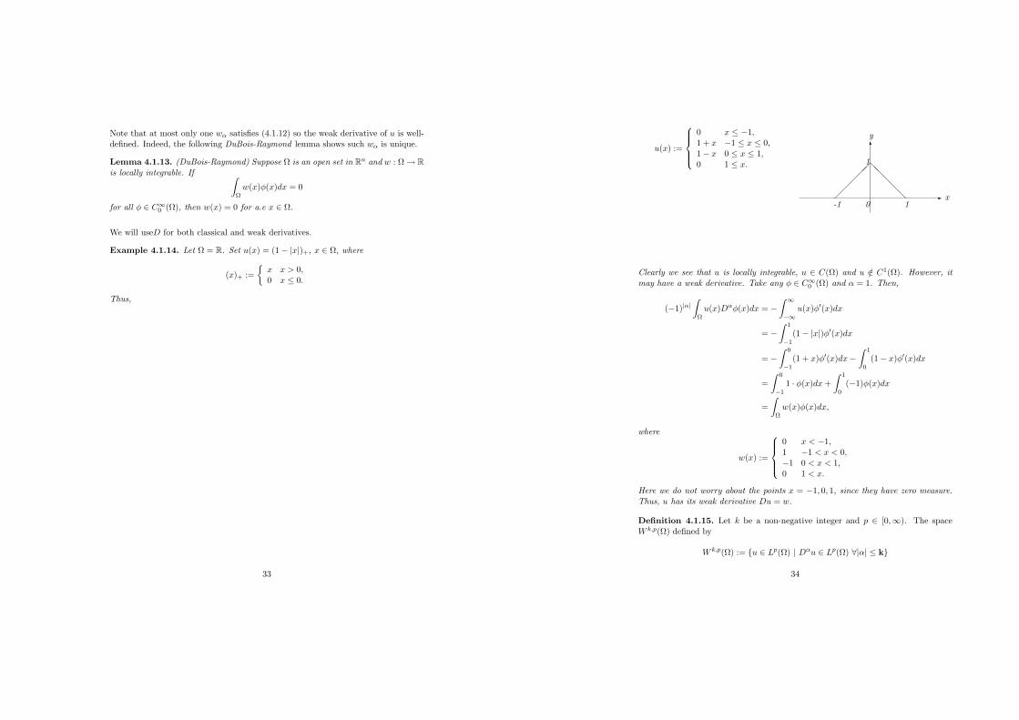
Example 4.1.14. Let ! = R. Set u(x) = (1+ |x|)+, x ! !, where
(x)+ :='
x x > 0,0 x $ 0.
Thus,
33
u(x) :=
#$$%
$$&
0 x $ +1,1 + x +1 $ x $ 0,1+ x 0 $ x $ 1,0 1 $ x.
!
"y
x##
###
$$
$$$
-1 10
1
Clearly we see that u is locally integrable, u ! C(!) and u /! C1(!). However, itmay have a weak derivative. Take any # ! C!
0 (!) and ! = 1. Then,
(+1)|!|(
!u(x)D!#(x)dx = +
( !
$!u(x)#%(x)dx
= +( 1
$1(1+ |x|)#%(x)dx
= +( 0
$1(1 + x)#%(x)dx+
( 1
0(1+ x)#%(x)dx
=( 0
$11 · #(x)dx +
( 1
0(+1)#(x)dx
=(
!w(x)#(x)dx,
where
w(x) :=
#$$%
$$&
0 x < +1,1 +1 < x < 0,+1 0 < x < 1,0 1 < x.
Here we do not worry about the points x = +1, 0, 1, since they have zero measure.Thus, u has its weak derivative Du = w.
Definition 4.1.15. Let k be a non-negative integer and p ! [0,,). The spaceW k,p(!) defined by
W k,p(!) := {u ! Lp(!) | D!u ! Lp(!) &|!| $ k}
34
is called a Sobolev space. It is a Banach space with the norm
)u)W k,p(!) :=
.
/!
|!|"k
)D!u)pLp(!)
0
11/p
.
Especially, when p = 2, we denote Hk(!) as W k,2(!). It is a Hilbert space with theinner product
-u, v.Hk(!) :=!
|!|"k
-D!u, D!v.L2(!).
Of special interest are H1(!) and H2(!). If ! = (a, b),( R, we see that
-u, v.H1(!) = -u, v.L2(!) + -Du,Dv.L2(!)
=( b
au(x)v(x)dx +
( b
aDu(x)Dv(x)dx.
-u, v.H2(!) = -u, v.L2(!) + -Du,Dv.L2(!) + -D2u, D2v.L2(!)
=( b
au(x)v(x)dx +
( b
aDu(x)Dv(x)dx +
( b
aD2u(x)D2v(x)dx.
Remark. 1) By using Holder’s inequality, we can prove Cauchy-Schwarz inequalityfor the inner product of Hk(!) as follows.
|-u, v.Hk(!)| $!
|!|"k
|-D!u, D!v.L2(!)|
$!
|!|"k
)D!u)L2(!))D!v)L2(!)
$2 !
|!|"k
)D!u)2L2(!)
2 !
|!|"k
)D!v)2L2(!)
= )u)Hk(!))v)Hk(!).
2) Let ! = (a, b) ( R and u ! H1(!). Then u ! C(!). In higher space dimensionsthis statement is no longer true.
4.2 One Dimensional Problem: Dirichlet condition
Let ! = (0, 1), p(·), q(·) ! C(!) and f(·) ! L2(!). Note that "! = {x = 0} %{ x =1}. We consider the following problem.
35
Find u : ! " R such that3+ d
dx(p
du
dx) + qu = f, x ! !,
u(x) = 0, x ! "!.(BVP)
Specifying the value of u at boundary points is said to be a Dirichlet boundarycondition. Now the methodology is
1) multiply the equation by a test function, integrate by parts and use boundaryconditions appropriately,
2) identify V , a(·, ·) and l(·),
3) verify, if possible, the assumptions of Lax-Milgram.
=# Unique existence to the variational formulation of the BVP.
Let # : ! " R be su"ciently smooth. We will call # our test function. Let us followthe methodology.
1)(
!f(x)#(x)dx =
(
!
*+ d
dx(p(x)
du(x)dx
)#(x) + q(x)u(x)#(x)+
dx
=4+p(x)
du(x)dx
#(x)5x=1
x=0
+(
!
*p(x)
du(x)dx
d#(x)dx
+ q(x)u(x)#(x)+
dx.
We want to eliminate the term [p(x)du(x)/dx#(x)]x=1x=0, so we suppose that the
test function # satisfies the same Dirichlet conditions as u, i.e, #(0) = #(1) = 0.Then we have that
(
!
*p(x)
du(x)dx
d#(x)dx
+ q(x)u(x)#(x)+
dx =(
!f(x)#(x)dx
for any test function #. We want u, v to be from the same space. For the term6! u#dx to make sense, we need u, # ! L2(!). For the derivatives du/dx, d#/dx
to make sense, we take this further, so u, # ! H1(!).
2) Let us chooseV :=
7# ! H1(!) | v(0) = v(1) = 0
8,
36
whereH1(!) =
7# ! L2(!) | D# ! L2(!)
8.
We equip the inner product -·, · V := -·, · H1(!). Let us define
a(u, v) :=(
!(pDuDv + quv)dx,
l(v) :=(
!fv dx.
Moreover, assume that p(x) ' p0 > 0, q(x) ' q0 > 0 for all x ! !.
3) We will verify the assumptions of Lax-Milgram’s theorem.
i) For # ! V and f ! L2(!), we see by Cauchy-Schwarz inequality that
|l(#)| = |(
!f#dx|
$ )f)L2(!))#)L2(!)
$ )f)L2(!) ()#)2L2(!) + )D#)2L2(!))
= cl)#)V ,
where we have set cl := )f)L2(!). Thus, l : V " R is bounded. Clearly l islinear, i.e, l(!# + $%) = !l(#) + $l(%) for any #, % ! V and !,$ ! R.
ii) Obviously a(·, ·) : V /V " R is bilinear. Moreover a(·, ·) is bounded. Indeed,
|a(#, %)| $ |(
!pD#D%dx| + |
(
!q#%dx|
$ maxx#!
|p(x)|(
!|D#D%|dx + max
x#!|q(x)|
(
!|#%|dx
$ maxx#!
|p(x)|)D#)L2(!))D%)L2(!) + maxx#!
|q(x)|)#)L2(!))%)L2(!)
$ C()D#)L2(!))D%)L2(!) + )#)L2(!))%)L2(!))
$ C,)D#)2L2(!) + )#)2L2(!)
,)D%)2L2(!) + )%)2L2(!)
= C)#)H1(!))%)H1(!),
where we have set
C := max{maxx#!
|p(x)|,maxx#!
|q(x)|}.
37
The bilinear form a(·, ·) is coercive, since for all # ! V
a(#, #) =(
!p|D#|2dx +
(
!q|#|2dx
' p0
(
!|D#|2dx + q0
(
!|#|2dx
= C)#)2V ,
where we have set C := min{p0, q0}.
We can now apply Lax-Milgram’s theorem to see that there uniquely exists asolution to the following problem
(P) Find u ! V such that(
!(pDuD# + qu#)dx =
(
!f#dx,
for any # ! V .
Remark. For V = H10 (!) we can use the norm ) ·) V defined by
)#)2V =(
!|D#|2dx,
since the following Poincare inequality holds:- there exists C > 0 such that(
!|#|2dx $ C
(
!|D#|2dx for &# ! V.
By using this inequality we can prove the unique existence of the solution solving(P) with q 0 0 in the same way as above.
4.3 One Dimensional Problem: Neumann condition
Let ! = (0, 1), p(x), q(x) ! C(!) and f(x) ! L2(!). We consider the followingproblem.
Find u : ! " R such that#$%
$&
+ d
dx
*pdu
dx
++ qu = f, x ! !,
d
dxu(x) = 0, x ! "!.
(NBVP)
38
Specifying the value of du/dx at boundary points is said to be a Neumann boundarycondition. We assume the same conditions for p, q as before, i.e, p(x) ' p0 > 0,q(x) ' q0 > 0 in !. Let us derive the variational form. Take a su"cient smoothtest function #, multiply (NBVP) by # and integrate.
(
!f(x)#(x)dx =
(
!
*+ d
dx
*p(x)
du(x)dx
+#(x) + q(x)u(x)#(x)
+dx
=4+p(x)
du(x)dx
#(x)5x=1
x=0
+(
!
*p(x)
du(x)dx
d#(x)dx
+ q(x)u(x)#(x)+
dx
=(
!
*p(x)
du(x)dx
d#(x)dx
+ q(x)u(x)#(x)+
dx.
We have eliminated the term [p(x)du(x)/dx#(x)]x=1x=0 by taking into account the Neu-
mann boundary conditions du(x)/dx = 0 for x = 0, 1. Let us choose the functionalspace V := H1(!) in this case and define
a(u, v) :=(
!(pDuDv + quv)dx,
l(v) :=(
!fv dx.
The corresponding variational problem is that:-
(P) Find u ! V such that(
!(pDuD# + qu#)dx =
(
!f#dx,
for any # ! V .
Again the linear form l(·) : V " R and the bilinear form a(·, ·) : V / V " R satisfythe assumptions of Lax-Milgram’s theorem, hence the problem (P) has the uniquesolution.
Remark. Consider (NBVP) with q 0 0. Then we see(
!f(x)dx = +
(
!
d
dx(p(x)
du(x)dx
)dx
=4p(x)
du(x)dx
5x=1
x=0
= 0.
39
Thus, we need to assume6! f(x)dx = 0 as a compatibility condition in this case. In
order to prove the unique existence of the solution, we need to modify the functionalspace. Let us define H1
m(!) by
H1m(!) := {# ! H1(!) |
(
!#dx = 0},
and equip the same inner product as H1(!). Again Poincare’s inequality is availablefor this space H1
m(!), i.e, for all # ! H1m(!)
(
!|D#|2dx $ C
(
!|#|2dx,
where C > 0 is a constant. By using this inequality we can prove the uniqueexistence of the solution solving (P) with q 0 0 and V = H1
m(!) in the same wayas above on the assumption
6! f(x)dx = 0.
4.4 One Dimensional Problem: Robin/Newton Condi-tion
Let ! = (0, 1), p(x), q(x) ! C(!), f(x) ! L2(!), &, g0, g1 ! R be constants. Weconsider the following problem. Find u : ! " R such that
#$$$$$%
$$$$$&
+ d
dx
*pdu
dx
++ qu = f, x ! !,
+pd
dxu(0) + &u(0) = g0,
pd
dxu(1) + &u(1) = g1.
(RNBVP)
Let us derive the variational form. Take su"ciently smooth #. This kind of boundarycondition is said to be a Robin/Newton boundary condition. We assume the sameconditions for p, q as before, i.e, p(x) ' p0 > 0, q(x) ' q0 > 0 in ! and that & ' 0.
(
!f(x)#(x)dx =
(
!
*+ d
dx
*p(x)
du(x)dx
+#(x) + q(x)u(x)#(x)
+dx
=4+p(x)
du(x)dx
#(x)5x=1
x=0
+(
!
*p(x)
du(x)dx
d#(x)dx
+ q(x)u(x)#(x)+
dx
= (+g1 + &u(1))#(1)+ (g0 + &u(0))#(0)
+(
!
*p(x)
du(x)dx
d#(x)dx
+ q(x)u(x)#(x)+
dx,
40
which is equal to(
!
*p(x)
du(x)dx
d#(x)dx
+ q(x)u(x)#(x)+
dx + &u(1)#(1) + &u(0)#(0)
=(
!f(x)#(x)dx+ g1#(1) + g0#(0).
This suggests that we should define a(·, ·), l(·) and the functional space V as follow-ing.
a(u, v) :=(
!(pDuDv + quv)dx + &u(1)v(1) + &u(0)v(0),
l(v) :=(
!fvdx+ g1v(1) + g0v(0),
V := H1(!).
As usual we need to show that the (bi)linear forms a, l are bounded and a is coer-cive to establish the unique solvability of (RNBV P ). Let us assume the followinginequality holds true for a while.
|#(x)| $ C)#)H1(!) (4.1)
for all # ! H1(!). Then it is easy to see that a(·, ·), l(·) are bounded. Now
a(#, #) ' min(p0, q0))#)2V + &(#(1)2 + #(0)2)
' min(p0, q0))#)2V= !)#)2V ,
where ! = min(p0, q0). Hence the bilinear form a becomes coercive and Lax-Milgram’s theorem assures the unique existence of the solution.
4.5 One Dimensional H1 inequalities
Here we derive some inequalities in the one dimensional case ! = (a, b). We definea function space H1
"0(!) by
H1"0(!) := {# ! H1(!) | #(a) = 0}.
The following inequality is one example of Poincare-Friedrichs inequality.
41
Proposition 4.5.1. For all # ! H1"0(!),
)#)L2(!) $112(b+ a))D#)L2(!).
Proof. We can write that for a $ &x $ b
#(x) =( x
aD#(')d'.
Then we see that
)#)2L2(!) =( b
a#(x)2dx
=( b
a
*( x
aD#(')d'
+2
dx
$( b
a
*( x
a12dx
+ *( x
aD#(')2d'
+dx
=( b
a(x+ a)
( x
aD#(')2d'dx
$( b
a(x+ a)
( b
aD#(')2d'dx
=12(b+ a)2)D#)2L2(a,b).
Example 4.5.2. We can apply this inequality to prove the unique solvability ofthe Dirichlet problem with a functional space V , a bilinear form a(·, ·) and a linearfunctional l(·) defined by
V := {# ! H1(0, 1) | #(0) = #(1) = 0},
a(u, v) :=( 1
0pDuDvdx for &u, v ! V,
l(u) :=( 1
0fudx for &u ! V.
We only check that the bilinear form a is bounded and coercive. We see that
|a(u, v)| $ supx#(0,1)
|p(x)|)Du)L2(!))Dv)L2(!) $ supx#(0,1)
|p(x)|)u)H1(!))v)H1(!)
42
and
a(v, v) ' p0)Dv)2L2(!)
=p0
2)Dv)2L2(!) +
p0
2)Dv)2L2(!)
' p0
2
9)Dv)2L2(!) +
2)v)2L2(!)
(b+ a)2
:
' !)v)2V ,
where ! := p0 min(1, 2/(b+ a)2)/2.
Proposition 4.5.3. The following Agmon’s inequality holds. For all # ! H1"0(!)
maxx#!
|#(x)|2 $ 2)#)L2(!))#)H1(!).
Proof.
#(x)2 =( x
a
d#(')2
d'd'
= 2( x
a#(')D#(')d'
$ 2*( x
a#(')2d'
+1/2 *( x
aD#(')2d'
+1/2
$ 2*( b
a#(')2d'
+1/2 *( b
aD#(')2d'
+1/2
$ 2)#)L2(!))#)H1(!),
which gives the inequality.
Noting that)#)L2(!) $
1b+ a max
x#[a,b]|#(x)|,
this Agmon’s inequality yields
maxx#!
|#(x)|2 $ 21
b+ a maxx#[a,b]
|#(x)|)#)H1(!),
ormaxx#!
|#(x)| $ 21
b+ a)#)H1(!)
for any # ! H1"0(!).
43
4.6 Weak Solutions to Elliptic Problems
The simplest elliptic equation is Laplaces’ equation:
#u = 0, (4.2)
where # :="n
j=1#2
#x2j
is the Laplace operator. A general second order ellipticequation is: given a bounded open set ! ( Rn find u such that:
+n!
i,j=1
"
"xj
*aij(x)
"u
"xi
++
n!
i=1
bi(x)"u
"xi+ c(x)u = f(x) x ! !, (4.3)
where classically aij ! C1(!), i, j = 1, . . . , n; bi ! C(!), i = 1, . . . , n; c ! C(!); f !C(!). For the equation to be elliptic we require
n!
i,j=1
aij(x)(i(j ' Cn!
i=1
(2i & ( = ((1, . . . , (n) ! Rn, (4.4)
where C > 0 is independent of x, (. Condition (4.4) is called uniform ellipticity.
The equation is usually supplemented with boundary conditions - Dirichlet, Neu-mann, Robin, or a mixed Dirichlet/Neumann boundary.
In the case of the homogeneous Dirichlet problem (u = 0 on "!) u is said to bea classical solution provided u ! C2(!) 2 C(!). Elliptic theory tells us that thereexists a unique classical solution provided aij , bi, c, f and "! are su"ciently smooth.However we are only intersted in problems where the data is not smooth, for examplef = sign(1/2 + |x|),! =( +1, 1). This problem can’t have u ! C2(!) because #uhas a jump discontinuity are |x| = 1/2. With the help of functional analysis theexistence/uniqueness theory for ‘weak’, ‘variational’ solutions turn out to be easyand is good for FEM.
4.7 Variational Formulation of Elliptic Equation: Neu-mann Condition
Let ! be a bounded domain in Rn with smooth boundary "!. Let p, q ! C(!) suchthat
p(x) ' p0 > 0, q(x) ' q0 > 0 &x ! !,
44
and f ! L2(!).
Find u : ! " R such that3 +3 · (p3u) + qu = f, x ! !,
"u
"n= 0, x ! "!,
(NBVP)
where n is the unit outward normal to the boundary "!. Note that
3 · (p3u) =n!
i=1
"
"xi
*p
"u
"xi
+
=n!
i=1
*p"2u
"x2i
+"p
"xi
"u
"xi
+
= p#u +3p ·3u,
"u
"n= 3u · n.
So we have a second order PDE. In one dimensional problem, in order to derive thevariational formulation we used integration by parts. Let us revise some formulaerelated to the integration by parts.
Notation:
3v =*
"v
"x1, . . . ,
"v
"x1
+T
3 ·3 v = 32v = #v
÷ ·A =n!
i=1
"Ai
"xi
(D2v)ij ="2v
"xi"xj
Tr(D2v) = #v.
Theorem 4.7.1 (Divergence theorem). Let A : ! " Rn be a C1 vector field. Thefollowing equality holds. (
!÷Adx =
(
#!A · nds.
45
Remark. Suppose A = fei with the coordinate vectorei = (0, · · · , 1, · · · , 0)T , i.e, the jth component is {ei}j = &i,j . Then we see
÷A ="
"xif.
So by the Divergence theorem(
!
"f
"xidx =
(
#!fnids.
In one dimensional case where ! = (a, b), "! = {a, b}, Divergence theorem becomes
( b
a
"f
"xdx = f(b)+ f(a).
Let us derive the integration by parts formula.
Proposition 4.7.1 (Integration by parts).For A ! C1(!; Rn), g ! C1(!),
(
!A ·3gdx =
(
#!gA · nds+
(
!g ÷ Adx.
Proof. By Divergence theorem we see that(
!÷(Ag)dx =
(
#!A · ngds.
Alternatively,÷(Ag) = g ÷ A + A ·3g.
By combining these equality we get the desired formula.
For example, if A = 3u and g = v, we have by integration by parts formula that(
!3u ·3vdx =
(
#!v3u · nds+
(
!v ÷ (3u)dx.
Noting that
3u · n ="u"n
and ÷ (3u) = !u,
46
where # is Laplacian, we obtain(
!v#udx =
(
#!v"u
"nds+
(
!3u ·3vdx.
Looking at our boundary value problem +÷ (p3u) + qu = f , we have that
+(
!÷(p3u)vdx =
(
!p3u ·3vdx+
(
#!p"u
"nvds.
Let v be a su"ciently smooth test function. Multiply (NBVP) by v and integrateusing Divergence theorem.
(
!fvdx =
(
!(+3 · (p3u) + qu)vdx
=(
!p3u3vdx+
(
#!p"u
"nvds +
(
!quvdx.
Since "u/"n = 0 on "!, we do not need to place a restriction on the test functionv. So if u solve (BVP), then
(
!(p3u3v + quv)dx =
(
!fvdx,
for any su"ciently smooth function v.
Now to use Lax-Milgram, we have to set up V , a(·, ·) and l(·). In order for the twoinner products on the left hand side to make sense, we take
V = H1(!),
a(u, v) =(
!(p3u3v + quv)dx,
l(v) =(
!fvdx,
for all u, v ! V . Note that V is a real Hilbert space with the norm
)v)V = )v)H1(!) =*(
!|3v|2dx +
(
!v2dx
+1/2
and obviously a(·, ·) : V / V " R is bilinear and l(·) : V " R is linear. Moreover
47
we observe
a(v, v) =(
!(p|3v|2 + qv2)dx
' p0
(
!|3v|2dx + q0
(
!v2dx
' min{p0, q0})v)2H1(!)
= !)v)2H1(!),
where we have put ! := min{p0, q0}. Thus a(·, ·) is coercive.
|a(v, w)| =--(
!(p3v ·3w + qvw) dx
--
$(
!(|p3u ·3w| + |qvw|)dx
$ C
(
!(|3v|2 + v2)1/2(|3w|2 + w2)1/2dx
$ C
*(
!(|3v|2 + v2)dx
+1/2 *(
!(|3w|2 + w2)dx
+1/2
= C)v)H1(!))w)H1(!).
Therefore, a(·, ·) is bounded. Finally let us check the boundedness of l(·).
|l(v)| =--(
!fvdx
--
$(
!|f ||v|dx
$*(
!f2dx
+1/2 *(
!v2dx
+1/2
= )f)L2(!))v)L2(!)
$ )f)H1(!))v)H1(!)
= Cl)v)H1(!).
Thus, l(·) is bounded. Now we can apply Lax-Milgram to prove that there exists aunique solution u ! V to the following problem (P).
(P) Find u ! V such thata(u, v) = l(v)
for all v ! V .
48
4.8 Variational Formulation of Elliptic Equation: Dirich-let Problem
On the same assumptions on !, p, q, f , we consider the following problem.
Find u : ! " R such that'+3 · (p3u) + qu = f, x ! !,u = 0, x ! "!,
(DBVP)
Let us derive the variational form of (DBVP) as in the section 2.5. Multiply (DBVP)by a su"ciently smooth test function v and integrate. Then we see
(
!fvdx =
(
!(p3u3v + quv)dx+
(
#!p"u
"nvdx.
Since we have u 0 0 on "!, we have to force our test function v to satisfy the samecondition; v 0 0 on "!. Then we obtain
(
!(p3u3v + quv)dx =
(
!fvdx
for any su"cient smooth function v with v 0 0 on "!. Set
V := {v ! H1(!) | v = 0 on "!}= H1
0 (!).
Note that V is a real Hilbert space with the inner product
-v, w.V := -3v,3w.L2(!) + -v, w.L2(!)
and )v)V = )v)H1(!). As before we define
a(v, w) :=(
!(p3v3w + qvw) dx,
l(v) =(
!fv dx.
The same argument as the previous section shows that a(·, ·) is a coersive andbounded bi-linear form and l(·) is a bounded linear functional on V . Therefore Lax-Milgram’s theorem tells us that there uniquely exists a solution to the variationalproblem of (DBVP).
49
4.9 Inhomogeneous Boundary Condition
Let V be a Hilbert space and a(·, ·) be a bilinear coercive form on V /V , let l(·) belinear, let V0 be a closed subspace of V and g ! V . Set Vg = {v ! V : v = v0+g, v0 !V0} and consider the problem: find u ! Vg such that a(u, v) = l(v) & v ! V0. Wecan show that there exists a unique solution.
Let u0 = u+ g. Then the problem becomes: find u0 ! V0 such that
a(u0) = l(v)+ a(g, v) & v ! V0. (4.5)
For the finite element method it becomes: find uh such that:
uh = g0#0 +M$1!
j=1
!j#j + g1#M . (4.6)
this means that A is the same as the homogeneous case but b now has contributionsfrom g0, g1.
4.10 Second Order Elliptic Problems
Consider the problem
+n!
i,j=1
"
"xj
*aij(x)
"u
"xi
++
n!
i=1
bi(x)"u
"xi+ c(x)u = f(x) &x ! ! (4.7)
with u = 0 on "!. Multiply by a test funciton and integrate by parts in the secondorder term using the divergence theorem. The result is the weak (variational) formof the BVP: find u ! V such that a(u, v) = l(v) & v ! V where V = H1
0 (!) and
a(w, v) :=n!
i,j=1
(
!aij(x)
"w
"xi
"v
"xj+
n!
i=1
(
!bi(x)
"w
"xiv(x) +
(
!c(x)w(x),
l(v) :=(
!f(x)v(x) = (f, v).
We seek to apply the Lax-Milgram theorem. Recall (v, w)H10 (!) =
6! vw +3v3w =
(v, w) + (3v,3w). We have three conditions to check to satisfy the theorem.
50
(1) Is l(·) a bounded linear functional? Clearly
l(!v + $w) = (f, !v + $w) = !(f, v) + $(f, w) = !l(v) + $l(w)
so l(·) is a linear functional on V and
|l(v)| =----(
!f(x)v(x) dx
---- $ )f)L2(!))v)L2(!) $ )f)L2(!))v)H10 (!)
where we have used the Cauchy-Schwartz inequality and thus l(·) is bounded.
(2) Is a(·, ·) bounded? Assume that )aij)L!(!), )bi)L!(!), )c)L!(!) are all boundedfor all i, j and that f ! L2(!). Then
|a(w, v)| $
------
n!
i,j=1
(
!aijwxivxj dx
------+
-----
n!
i=1
(
!biwxiv dx
----- +----(
!cwv dx
----
$n!
i,j=1
maxx#!
|aij(x)|(
!|wxi ||vxj | dx +
n!
i=1
maxx#!
|bi(x)|(
!|wxi ||v| dx + max
x#!|c(x)|
(
!|w||v| dx
$ c
.
/n!
i,j=1
(
!|wxi ||vxj | dx +
n!
i=1
(
!|wxi ||v| dx +
(
!|w||v| dx
0
1
$ c
.
/n!
i,j=1
)wxi))vxj)+n!
i=1
)wxi))v)+ )w))v)
0
1
$ c
.
/n!
i,j=1
)w)V )v)V +n!
i=1
)w)V )v)V + )w)V )v)V
0
1
= c1)w)V )v)V
where c = max{maxij max! |aij(x)|,maxi max! |bi(x)|,max! |c(x)|} and c1 = c(n2+n + 1).
(3) Is a(·, ·) coercive? The crucial assumption is that the aij satisfies the ellipticityassumption
n!
i,j=1
aij(x)(i(j ' cn!
i=1
(2i & ((1, . . . , (n) ! Rn, &x ! !, (4.8)
i.e. for all x ! ! we must have
(T A(x)( ' c)()2 = (T (. (4.9)
51
We also assume that
c(x)+ 12
n!
i=1
"bi(x)"xi
' 0&x ! !. (4.10)
Then
a(v, v) =n!
i,j=1
(
!aij(x)vxivxj +
n!
i=1
(
!bi(x)vxiv +
(
!c(x)v(x)2
' c
(
!
n!
i=1
v2xi
+n!
i=1
(
!bi(x)
"v2/2"xi
+(
cv2.
The middle integral here is 12
6! b · 3(v2), which after integration by parts equals
+12
6! v23 · b so that
a(v, v) ' cn!
i=1
(
!v2xi
+(
!v2(c(x)+ 1
23 · b(x))
' cn!
i=1
(
!v2xi
= c)3v)2
Note that we need 3 · b ! L!(!) for this to work. We wish to show that
a(v, v) ' c0)v)2V = c0()v)+ )3v)). (4.11)
Recall the Poincare-Friedrichs inequalities
)v)2 $ c&)3v)2 & v ! H10 (!).
Hence
a(v, v) ' c)3v)2 ' c
c&)v)
12a(v, v) +
12a(v, v) ' c
2)3v)2 +
c
2c&)v)
' c0;)3v)2 + )v)2
<
4.10.1 Remarks on the Lax-Milgram Result
1. Uniqueness: by our usual methods this follows from the linearity of l(·), thebilinearity of a(·, ·) and the coercivity of a(·, ·).
52
2. Stability estimate: we know that
c0)u)2V $ a(u, u) = l(u) $ c2)u)V
so we can deduce that the solution to our BVP satisfies
)u)H1(!) $1c0)f)L2(!). (4.12)
3. Continuity with repsect to l(·). Consider the two problems
u1 ! V s.t. a(u1, v) = l1(v) & v ! V
u2 ! V s.t. a(u2, v) = l2(v) & v ! V.
Thena(u1 + u2) = l1(v)+ l2(v) = l(v). (4.13)
Choosing v = u1 + u2:
c0)u1 + u2)2V = l(u1 + u2) $ )l1 + l2)V ")u1 + u2)
# )u1 + u2)V $)l1 + l2)V "
c0
In terms of our original elliptic bvp’s we have that
)u1 + u2)H1(!) $1c0)f1 + f2)L2(!). (4.14)
4. If l is the zero element of V & (i.e. l(v) = 0 & v ! V ) then 0 = a(u, u) #)u)V = 0 by coercivity and u = 0.
4.10.2 Inhomogeneous Boundary Conditions
Consider the elliptic problem
+3 · (p3u) + qu = f x ! ! (4.15)u = g x ! "! (4.16)
where ! is a bounded open subset of R2. We assume that the data p, q, f, g aresu"ciently smooth and that
pM ' p(x) ' p0 > 0 &x ! !qM ' q(x) ' q0 > 0 &x ! !
53
Let v be a test function. Multiply by v and integrate:
0 = +(
!v3 · (p3u) +
(
!quv +
(
!fv
= I1 + I2 + I3
Nov choosing ) = v, f = p3u in:
3 · ()f) = )3 · f +3) · f3 · (vp3u) = v3 · (p3u) +3v · p3u
I1 = +(
!3 · (vp3u)+3v · p3u
=(
!p3v ·3u+
(
#!vp3u · *
Choosing v = 0 on "! we have I1 =6! p3v ·3u. Thus
0 =(
!p3v ·3u + quv + fv & v ! H1
0 (!). (4.17)
Set V0 = H10 (!), a(u, v) =
6! p3v · 3u + quv, l(v) =
6! fv. Note that u *! V0.
However g ! H1(!) so u+ g ! H1(!) and u+ g ! H10 (!) = V0, i.e u ! Vg := {w !
V = H1(!) : w = g + v, v ! V0}.
Thus our variational problem (P ) is to find u ! Vg such that a(u, v) = l(v) & v ! V0.Observe that V0 is a linear space but Vg = g + V0 is an a"ne space. We can’t applyLax-Milgram directly. Consider u& = u+ g ! V0:
a(u& + g, v) = a(u, v) = l(v) & v ! V0
so u& ! V0 solves
a(u&, v) = l(v)+ a(g, v) =: l&(v) & v ! V0
Now we just need to check Lax-Milgram for this problem. Clearly a(·, ·) is bilinear(and symmetric). Coercivity:
a(v, v) =(
!p|3v|2 + qv2 ' p0
(
!|3v|2 + q0
(
!v2 ' min(p0, q0)
(
!|3v|2 + v2 ' c0)v)H1(!).
Boundedness: using the Cauchy-Schwartz inequality we have
|a(w, v)| =----(
!p3w3v + qwv
---- $ pM
(
!|3w||3v| + qM
(
!|w||v|
$ max(pM , qM )()3w))3v)+ )w))v))$ c)w)H1(!))v)H1(!).
54
Clearly l& is linear and
|l&(v)| = |l(v)+ a(g, v)| $| l(v)| + |a(g, v)| $ )f))v)+ c)g)H1(!))v)H1(!) $ L&)v)H1(!).
Thus there exists a unique u& and we conclude therefore that there exists a uniqueu = u& + g.
The bilinear form is symmetric so there is an energy and associated minimisationproblem:
J(v) =12a(v, v)+ l(v)
Find u ! Vg s.t. J(u) $ J(v) & v ! Vg.
Exercise: Prove that these two problems are equivalent.
4.11 Finite Element Method in 2D
Take ! to be a polygon. Let Th be a triangulation of !, Th = {+} and set h$ =diam+ (the length of the longest side), h = maxdiam +. We assume that |Th| < ,.Any triangles in Th must intersect along a complete edge, at a vertex of not at all.
Note that any linear function on R2 is of the form v(x, y) = a+bx+cy and is definedby three parameters. Thus any function
vh ! Vh := {' ! C(!) : vh|$ is linear} (4.18)
is uniquely determined by it values at the vertices of the triangulation:
#i(xj) = &ij i, j = 1, . . . , Nh, xj is a triangle vertex. (4.19)
The support of the basis functions is local, so A will again be sparse.
Example 4.11.1. Find u ! H1(! such that(
!p3u3v + quv dx =
(
!fv dx & v ! H1(!). (4.20)
A finite element method applied to this yields the problem: find uh ! H1(!) suchthat (
!p3uh3vh + quhvh dx =
(
!fvh dx & vh ! Vh. (4.21)
55


![Modern Computational Statistics [1em] Lecture 13: Variational … · 2020-05-27 · Modern Computational Statistics Lecture 13: Variational Inference Cheng Zhang School of Mathematical](https://static.fdocument.org/doc/165x107/5f4b685473300c10ae514129/modern-computational-statistics-1em-lecture-13-variational-2020-05-27-modern.jpg)