The marginal utility of money:

A modern Marshallian approach to consumer choice∗

Daniel Friedman

University of California at Santa Cruz

Jozsef Sakovics

The University of Edinburgh

July 19, 2011

Abstract

We reformulate neoclassical consumer choice by focusing on λ, the marginal utility

of money. As the opportunity cost of current expenditure, λ is approximated by the

slope of the indirect utility function of the continuation. We argue that λ can largely

supplant the role of an arbitrary budget constraint in partial equilibrium analysis. The

result is a better grounded, more flexible and more intuitive approach to consumer

choice.

JEL classification: D01, D03, D11.

Keywords: budget constraint, separability, value for money.

∗We thank Luciano Andreozzi, Axel Leijonhufvud, Carmen Matutes, Ryan Oprea, Nirvikar Singh, Donald

Wittman and other June 2011 UCSC brown bag seminar participants for helpful suggestions, and thank Olga

Rud for help in preparing the figures.

1

1 Introduction

When faced with the simple task of deciding how much to buy of a particular good at a

given price, Homo Economicus solves a horrendously complex problem. She maximizes her

utility by choosing a lifetime consumption plan that takes into consideration all the contin-

gencies she might face in the immediate and distant future (as well as frictions, asymmetric

information, and other complications), and then executes the first component of this plan

by purchasing the optimal amount of the good in question.

Not surprisingly, economists have found ways to make consumer choice theory more

tractable. The textbook approach assumes, explicitly or implicitly, that the good in question

has at most a few substitutes and complements, and chops off this small portion of the

lifetime problem. To this portion it applies a budget constraint, and analyzes the budget-

constrained consumer’s reaction to surprises in prices and availability of the target good and

related goods, as well as to unplanned changes in the budget itself (e.g., Hal Varian, 1992,

Ch. 7-8).

Unfortunately the textbook analysis has serious shortcomings. By fully separating the

subproblem from the larger problem, the budget constraint rules out substitution of pur-

chasing power across the boundary, irrespective of the realization of prices, etc. As we will

see, a fixed budget constraint distorts the solution because the size of the optimal budget

is highly sensitive to variations in the subproblem. One could mitigate the distortion by

broadening the subproblem – perhaps to a set where a bona fide liquidity constraint binds –

but that would forfeit the simplicity of partial equilibrium and would tie together decisions

over goods whose consumption utilities are independent of each other. Thus standard partial

equilibrium analysis does violence to the underlying general equilibrium problem, but it is

widely accepted that this is the price that must be paid for tractability.

This essay will challenge that view. We argue for a robust, flexible and natural approach

to disaggregation, simpler than the textbook approach but no less rigorous. The basic

idea is to use the marginal utility of money, rather than the budget constraint, to link the

subproblem to the rest-of-life problem. Using a cardinal utility function, the consumer can

react to changes in the environment by substituting optimally within the subproblem and

also by optimally shifting purchasing power across the subproblem boundary. The marginal

2

utility of money provides a robust criterion for the trade-off between subproblem and rest-

of-life, and it resonates with the findings of consumer research.

Section 2 presents a standard general equilibrium formulation of the consumer’s life-

time problem, and offers a simple definition of separable subproblems. After reviewing the

textbook approach to the subproblem, it shows how our new Marshallian approach offers

a somewhat different solution. The next section compares textbook comparative statics to

those of the new Marshallian approach: the substitution effect is the same, but income effects

and overall effects differ.

Section 4 then extends the new Marshallian approach to indivisible goods, and to larger

subproblems. It shows how the consumer can use personal experience to update the marginal

utility of money without trying to resolve the entire lifetime problem. The section also

shows how to model liquidity-constrained consumers, including those who live paycheck to

paycheck.

Section 5 discusses further applications of the new Marshallian approach. The marginal

utility of money provides a simple heuristic that seems consistent with descriptions of con-

sumer behavior in the marketing literature, and is a useful counterpoint to the behavioral

economics notion of mental accounting. Somewhat more speculatively, the section proposes

connections to the management of multidivisional firms and to money illusion.

A concluding discussion reiterates that, compared to the textbook approach, the new

Marshallian approach offers (a) more robust prescriptions for how consumers should react

to surprises, (b) a better way to connect partial equilibrium to general equilibrium analysis,

and also (c) more plausible descriptions of actual human behavior.

An historical perspective may be helpful before we begin. The idea of a cardinal utility

function defined over purchasing power goes back at least to Jeremy Bentham (1802), as does

the argument that marginal utility diminishes. Alfred Marshall (1890, 1920), synthesizing

the work of earlier Marginalists, obtained the crucial first order condition (that marginal

utility for each good equals its price times the marginal utility of money) in the special case

that total utility is additively separable in each good. “Edgeworth destroyed this pleasant

simplicity and specificity when he wrote the total utility function as f(x1, x2, x3, ...),” says

George Stigler (1950, p. 322). It fell to John Hicks and Roy Allen (1934) to show how to

3

impose a budget set to derive demand functions and cross-price elasticities when goods might

have complements and substitutes. Their analysis, developed further by Paul Samuelson and

a host of other economists, eventually became textbook orthodoxy.

We present a model in the spirit of Marshall that can deal with Edgeworth’s complica-

tions. The model uses cardinal utility to obtain price elasticities that closely approximate

the general equilibrium elasticities.

2 The consumer choice problem

We begin by showing how to separate a tractable subproblem from the horrendously complex

lifetime choice problem, and then distinguish our new Marshallian solution of the subproblem

from the textbook solution.

2.1 A subproblem of the lifetime problem

Let X ∈ <N represent an agent’s lifetime plan of work and consumption. Using the notation

x−i = min{0, xi} ≤ 0 and x+i = xi − x−i = max{0, xi} ≥ 0, work is represented by the

negative components X− = (x−1 , ..., x−N) – analogous to inputs of a production function –

and consumption by the positive components X+ = (x+1 , ..., x+N) – analogous to outputs, with

investment in human capital included. Of course, the number N of goods is astronomically

large, especially if we follow Arrow and Debreu in indexing goods separately by location,

date and (for unresolved contingencies) the realized state of Nature.

The agent takes as given a price vector P ∈ <N+ , and has preferences represented by

a utility function U defined over a set that contains all feasible plans. “Feasible” means

that X satisfies any relevant technological constraints (e.g., that a day’s activities can be

done in 24 hours) and also that it satisfies PX =∑N

i=1 PiXi = 0. That is (after including

special sorts of work such as selling endowed assets and special sorts of consumption such as

taxes and gifts), lifetime income −PX− > 0 equals lifetime expenditure PX+. Sometimes

it will be convenient also to refer to exogenous transfers of purchasing power by changing

the endowment of good i = 0, whose price P0 is normalized to 1.

4

Assume for now (later we will relax this) that all purchasing power is liquid: L = x0 −PX− > 0 is available without further constraint. Letting ξ(L, P ) denote the set of feasible

plans, the indirect lifetime utility function is

Vo(L, P ) = maxU(X) s.t. X ∈ ξ(L, P ). (1)

A consumer subproblem is to choose an n-subvector of the consumption vector X+ of a

lifetime plan X. By rearranging the indexing, we can write the subvector as x ∈ ξ[n](L, P ) ⊂<n+ and the rest of the life plan as X⊥ = (x0, 0, ..., 0, xn+1, xn+2, ..., xN) ∈ ξ⊥(L, P ), where

ξ[n](L, P ) denotes the n-subvectors of ξ, and ξ⊥(L, P ) denotes the complementary subvectors.

The corresponding price subvector of P is denoted p ∈ <n+. Typically n is small, perhaps

just 1 or 2.

The subproblem is separable if, for some utility function u defined on Rn+ we can, with

negligible error, write

U(X) = u(x) + U(X⊥) (2)

for any feasible plan X. A sufficient condition for separability is that the cross second partial

derivative Uij = 0 everywhere for all i = 1, ..., n and j = n+ 1, ..., N .

Substituting equation (2) into (1), we have the following recursion:

Vo(L) = maxx∈ξ[n]

{u(x) + V (L− px)} , (3)

where V (L) denotes the rest-of-life indirect utility function, defined as in (1) but with X

restricted to ξ⊥(L, P ). The dependence on the rest-of-life prices P⊥ is suppressed in order

to emphasize the impact of the subproblem price vector p. The equation says that if today’s

subproblem is separable, then the only effect today’s consumption has on subsequent utility is

via today’s expenditure px =∑n

i=1 pixi, which reduces the consumer’s subsequent purchasing

power. Of course, the subproblem need not be separated chronologically, but if it is then (3)

can be regarded as a Bellman equation with discounting built into P⊥.

Thus the consumer’s subproblem is to choose her optimal basket of n goods that have

possibly interdependent consumption values, but that are separable from the consumption

values of all other goods.

5

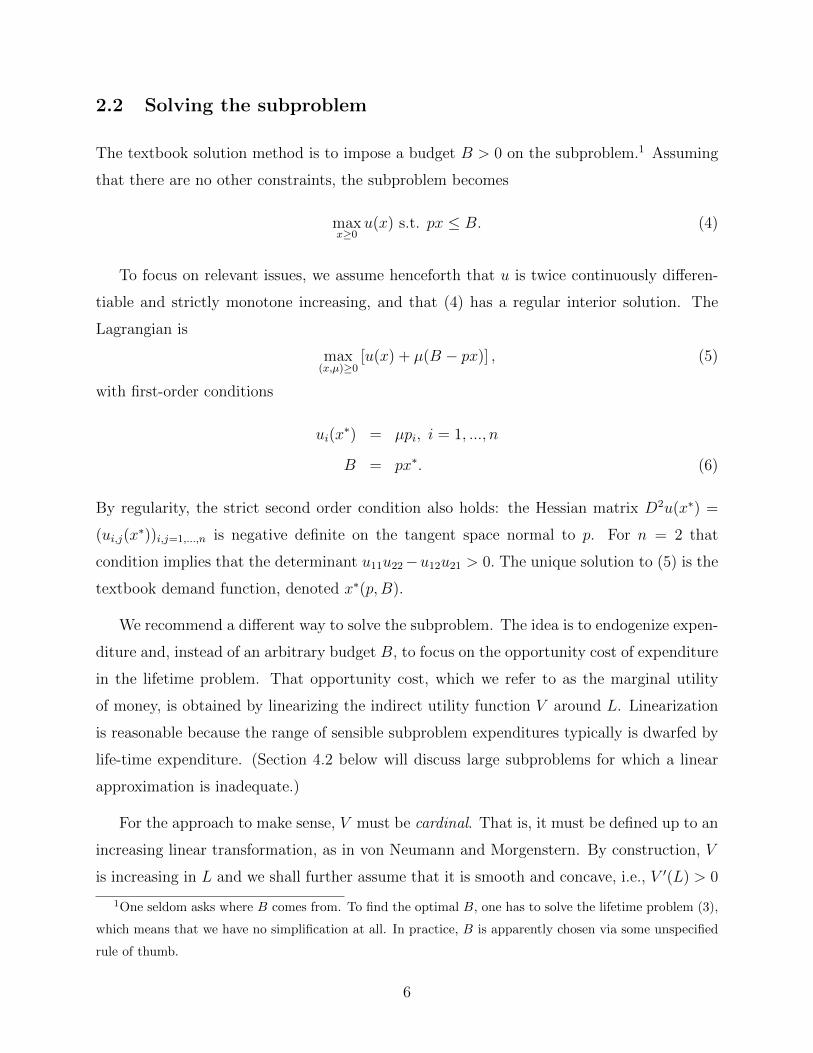
2.2 Solving the subproblem

The textbook solution method is to impose a budget B > 0 on the subproblem.1 Assuming

that there are no other constraints, the subproblem becomes

maxx≥0

u(x) s.t. px ≤ B. (4)

To focus on relevant issues, we assume henceforth that u is twice continuously differen-

tiable and strictly monotone increasing, and that (4) has a regular interior solution. The

Lagrangian is

max(x,µ)≥0

[u(x) + µ(B − px)] , (5)

with first-order conditions

ui(x∗) = µpi, i = 1, ..., n

B = px∗. (6)

By regularity, the strict second order condition also holds: the Hessian matrix D2u(x∗) =

(ui,j(x∗))i,j=1,...,n is negative definite on the tangent space normal to p. For n = 2 that

condition implies that the determinant u11u22−u12u21 > 0. The unique solution to (5) is the

textbook demand function, denoted x∗(p,B).

We recommend a different way to solve the subproblem. The idea is to endogenize expen-

diture and, instead of an arbitrary budget B, to focus on the opportunity cost of expenditure

in the lifetime problem. That opportunity cost, which we refer to as the marginal utility

of money, is obtained by linearizing the indirect utility function V around L. Linearization

is reasonable because the range of sensible subproblem expenditures typically is dwarfed by

life-time expenditure. (Section 4.2 below will discuss large subproblems for which a linear

approximation is inadequate.)

For the approach to make sense, V must be cardinal. That is, it must be defined up to an

increasing linear transformation, as in von Neumann and Morgenstern. By construction, V

is increasing in L and we shall further assume that it is smooth and concave, i.e., V ′(L) > 0

1One seldom asks where B comes from. To find the optimal B, one has to solve the lifetime problem (3),

which means that we have no simplification at all. In practice, B is apparently chosen via some unspecified

rule of thumb.

6

and V ′′(L) ≤ 0 for L in the relevant range. A sufficient condition is that, analogous to

production functions, U is smooth, monotone, and exhibits decreasing returns to scale in

relevant regions.

Thus a preliminary step is to take the first-order Taylor approximation of the indirect

utility function for the lifetime problem. Defining λ = V ′(L) as the marginal utility of money,

we have

V (L− px) ≈ V (L)− λpx for px << L. (7)

Substituting the linearization (7) into the lifetime optimization problem (3) and dropping

the constant term V (L), we obtain the subproblem objective function, which is subject to

no further constraint

maxx≥0

[u(x)− λxp] . (8)

In the subproblem (8), the parameter λ is exogenous, and the equation invites alternative

characterizations of its role. Thus the marginal utility of money may also be thought of as

the opportunity cost of today’s expenditure, or the “shadow utility” of purchasing power,

or the “conversion rate” between utility and money. Note that λ depends only on V and

L, and is independent of u and p in any small subproblem. Indeed, the same value of λ

applies to any subproblem, as long as the linear approximation (7) is valid. By contrast, the

optimal choice of the exogenous parameter B in the standard approach is intimately tied to

the characteristics of the subproblem and hence is much less robust. We will elaborate this

point in Section 3.2 below.

Again assuming a regular interior solution, the first-order conditions for (8) are

ui(x∗) = λpi, i = 1, ..., n. (9)

We denote the “Marshall-Edgeworth” demand function resulting from the solution of (9) by

M(p, λ). Of course, from (9) one can still recover the usual textbook tangency condition that

for any pair of the n goods in the optimal bundle, the marginal rate of substitution is equal

to the price ratio. Here it is the constant marginal utility of money that gives us that result,

rather than a fixed budget.

7

3 Comparing solutions

Observe that (9) is the same as (6) except that λ replaces µ and the budget constraint is

dropped. Dropping one equation makes sense because λ is exogenous in subproblem (8).

But what is the relation between the marginal utility of money, λ, and the shadow price of

the budget constraint, µ? Recall that µ is the marginal consumption utility of a dollar spent

over the budget. If B is not chosen optimally for the lifetime problem (3), then µ differs

from the true marginal cost of overspending, V ′(L− B) ≈ V ′(L) = λ. Thus one can regard

µ as an estimate of λ, where the quality of the estimate depends on the quality of the choice

of the budget.

x2

x1 x1*

x2*

B

IEP

expenditure

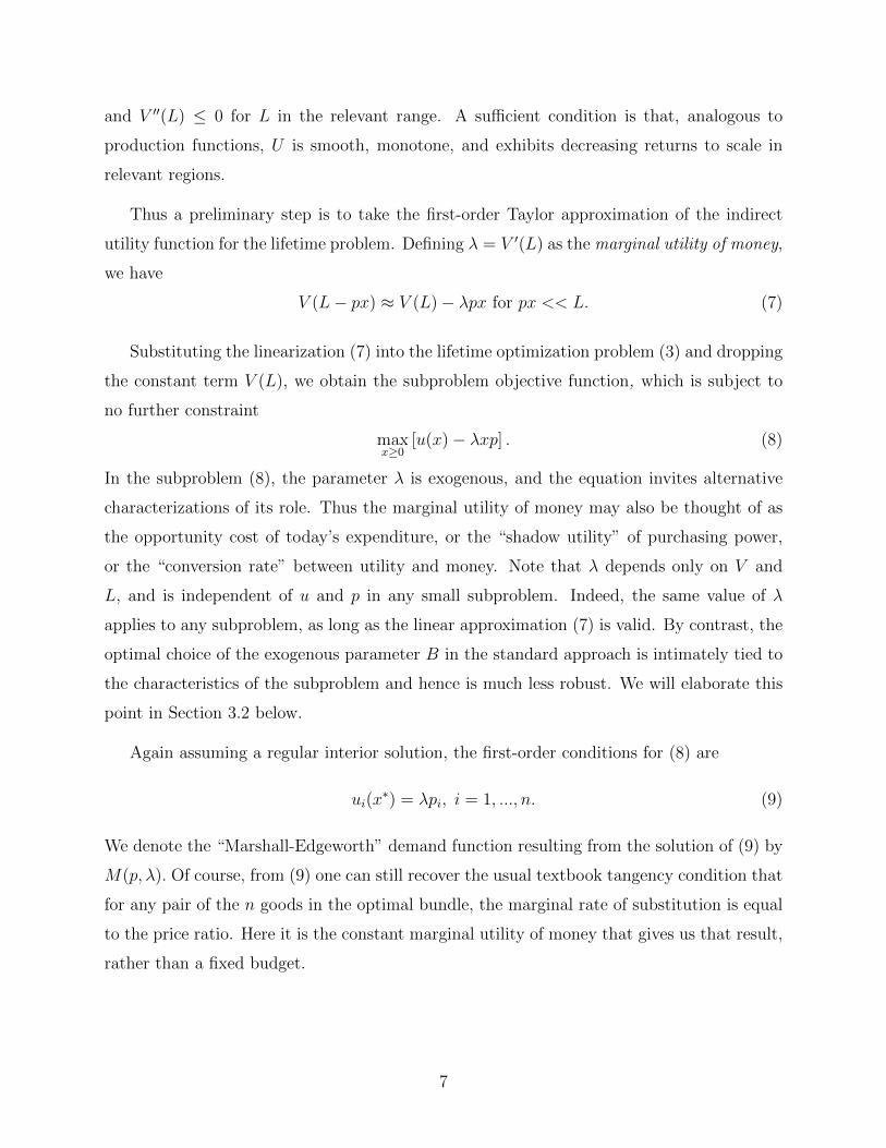
Figure 1: Optimal consumption with fixed budget B. The curve in the lower quadrant shows

expenditure e(x) along the IEP as a function of consumption x1 of the first good. Given B > 0 on

the (downward pointing) vertical axis, one finds the corresponding point on the expenditure curve

to locate optimal consumption x∗1 of good 1 on the horizontal axis, and then uses the IEP in the

upper quadrant to locate x∗2 on the (upward pointing) vertical axis.

The two approaches are connected via the Income Expansion Path (IEP), the locus of

points that satisfy the tangency conditions (6) for a given price vector as B varies from zero

to infinity. Since the tangency conditions are the same in (9), viz., that the price ratio equals

the marginal rate of substitution, exactly the same locus of utility maximizing bundles is

traced out by (9) as λ varies from infinity to zero.

Consequently, for any price vector p, the textbook demand function x∗(p,B) and the

8

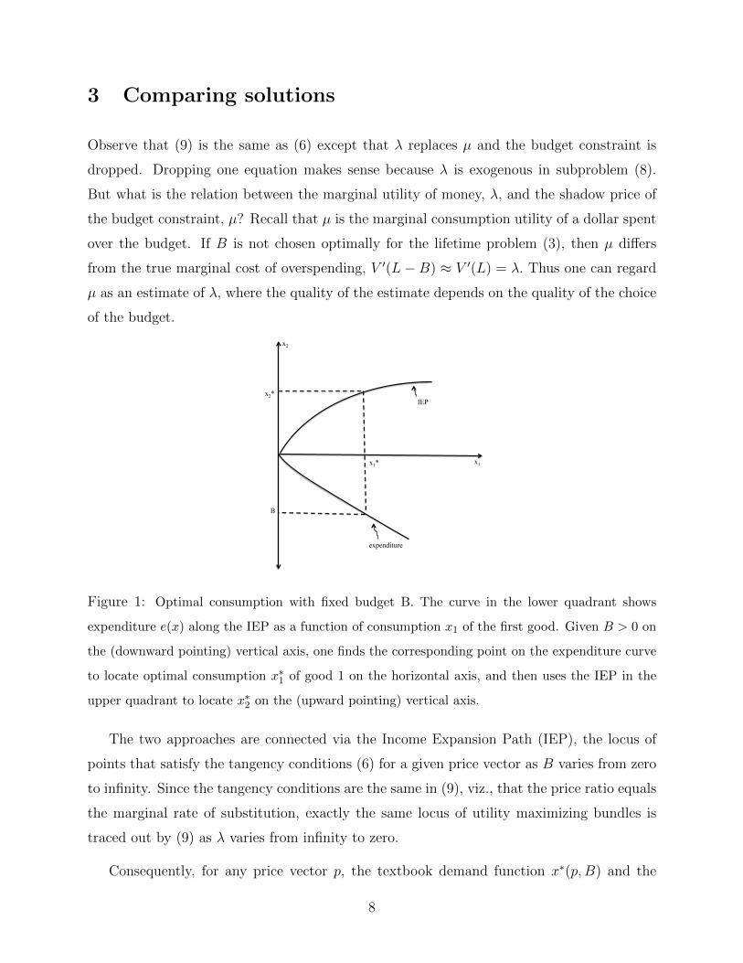
Marshall-Edgeworth demand function M(p, λ) both pick out points on the same IEP. The

earlier discussion shows that the two different decision rules will typically select different

points on this IEP. Figure 1 illustrates the choice of x∗(p,B), and Figure 2 also illustrates

the choice of M(p, λ). The intuition for M(p, λ) is that the consumer moves up the IEP as

long as the utility gain exceeds the opportunity cost of the expenditure, and stops when the

gain diminishes to the point that it is equal to the opportunity cost.

x2*

x2

x1

M2

x1*

e(x)

B

λp2

IEP

u2(x*) M1

expenditure

Figure 2: Optimal consumption with given λ. The curve above the leftward pointing horizontal axis

shows the marginal utility for good 2 as a function of its consumption along the IEP (see Appendix

A for its derivation). Given λ > 0 and price p2, one locates their product on that horizontal axis,

finds the corresponding point on the marginal utility curve, and reads off the vertical axis the

optimal consumption M2 of good 2. Using the IEP in the first quadrant, one then locates M1 on

the rightward pointing horizontal axis. In this example, the budget B encourages the consumer to

overspend relative to the lifetime optimal plan.

9

3.1 Comparative statics

Let us see how consumers using the λ rule react to small changes in the subproblem, and how

those reactions compare to those of consumers using the budget rule. During this exercise

we hold λ constant, so the elasticities should be regarded as short run.

Income elasticity under the λ rule is trivially zero as long as the consumer is not liquidity

constrained. Since she can freely shift purchasing power across the boundary of the sub-

problem, a marginal shift in income tentatively allocated to the subproblem has no effect on

λ and thus no effect on choice. To call out this simple but important observation, we write

Proposition 1. The (short term) income elasticity of Marshall-Edgeworth demand M(p, λ)

is zero when the consumer faces no liquidity constraints.

Now consider price effects. In the case n = 1, we have (in current notation) M(p1, λ) =

(u1)−1(λp1), or using Marshall’s enduring convention of putting price on the vertical axis

and quantity on the horizontal axis, the demand curve is simply p1 = u1(x1)λ

. As Marshall

explained long ago, one increases consumption of the good until the marginal utility falls to

the price scaled by the marginal utility of money.

The same intuition applies to the general case, except that one increases consumption

of baskets along the IEP. The impact of a change in a single price is complicated by the

implied move to a different IEP. The general case n > 1 is a bit awkward to state, but is

nicely illustrated in the following result for n = 2.

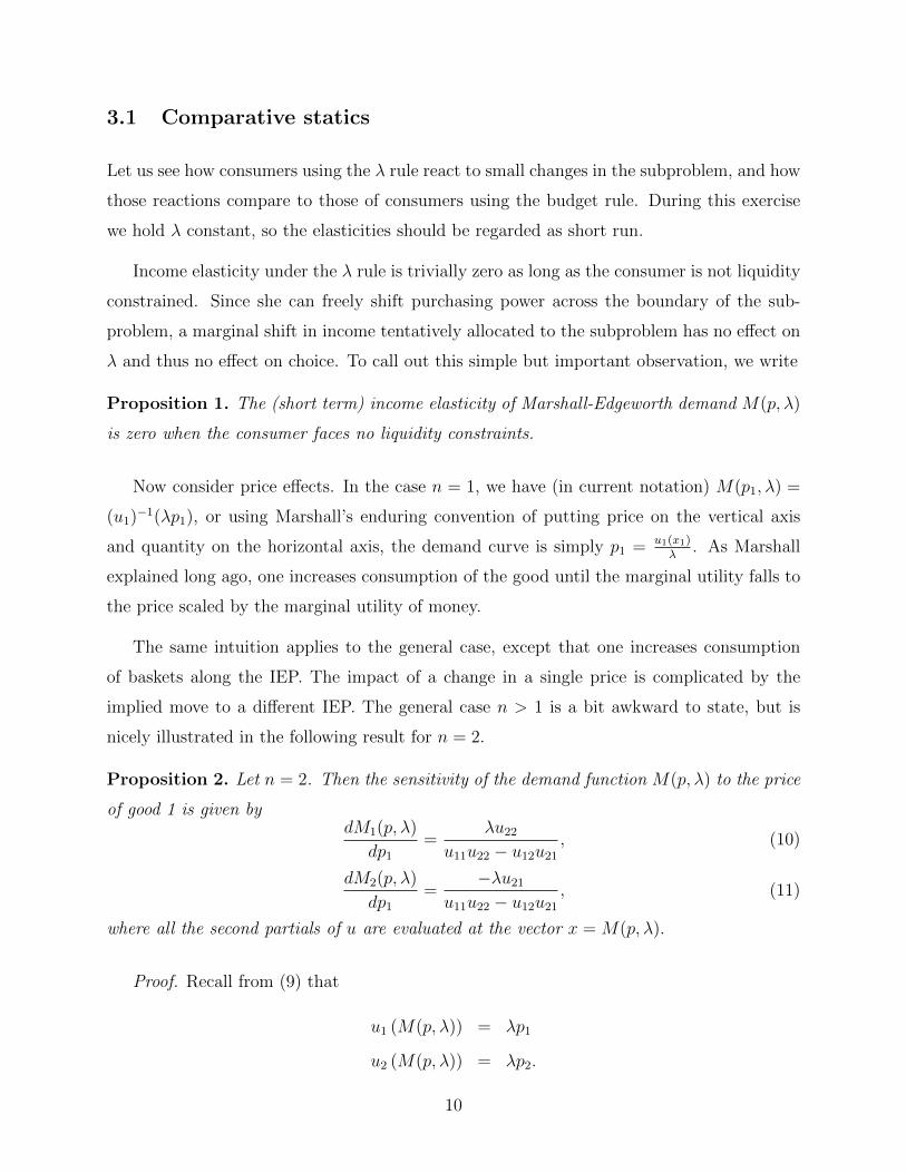
Proposition 2. Let n = 2. Then the sensitivity of the demand function M(p, λ) to the price

of good 1 is given bydM1(p, λ)

dp1=

λu22u11u22 − u12u21

, (10)

dM2(p, λ)

dp1=

−λu21u11u22 − u12u21

, (11)

where all the second partials of u are evaluated at the vector x = M(p, λ).

Proof. Recall from (9) that

u1 (M(p, λ)) = λp1

u2 (M(p, λ)) = λp2.

10

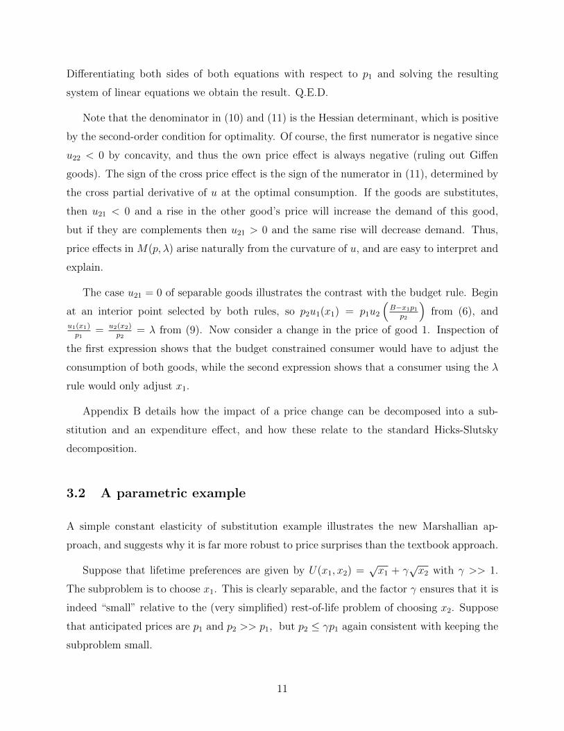
Differentiating both sides of both equations with respect to p1 and solving the resulting

system of linear equations we obtain the result. Q.E.D.

Note that the denominator in (10) and (11) is the Hessian determinant, which is positive

by the second-order condition for optimality. Of course, the first numerator is negative since

u22 < 0 by concavity, and thus the own price effect is always negative (ruling out Giffen

goods). The sign of the cross price effect is the sign of the numerator in (11), determined by

the cross partial derivative of u at the optimal consumption. If the goods are substitutes,

then u21 < 0 and a rise in the other good’s price will increase the demand of this good,

but if they are complements then u21 > 0 and the same rise will decrease demand. Thus,

price effects in M(p, λ) arise naturally from the curvature of u, and are easy to interpret and

explain.

The case u21 = 0 of separable goods illustrates the contrast with the budget rule. Begin

at an interior point selected by both rules, so p2u1(x1) = p1u2

(B−x1p1

p2

)from (6), and

u1(x1)p1

= u2(x2)p2

= λ from (9). Now consider a change in the price of good 1. Inspection of

the first expression shows that the budget constrained consumer would have to adjust the

consumption of both goods, while the second expression shows that a consumer using the λ

rule would only adjust x1.

Appendix B details how the impact of a price change can be decomposed into a sub-

stitution and an expenditure effect, and how these relate to the standard Hicks-Slutsky

decomposition.

3.2 A parametric example

A simple constant elasticity of substitution example illustrates the new Marshallian ap-

proach, and suggests why it is far more robust to price surprises than the textbook approach.

Suppose that lifetime preferences are given by U(x1, x2) =√x1 + γ

√x2 with γ >> 1.

The subproblem is to choose x1. This is clearly separable, and the factor γ ensures that it is

indeed “small” relative to the (very simplified) rest-of-life problem of choosing x2. Suppose

that anticipated prices are p1 and p2 >> p1, but p2 ≤ γp1 again consistent with keeping the

subproblem small.

11

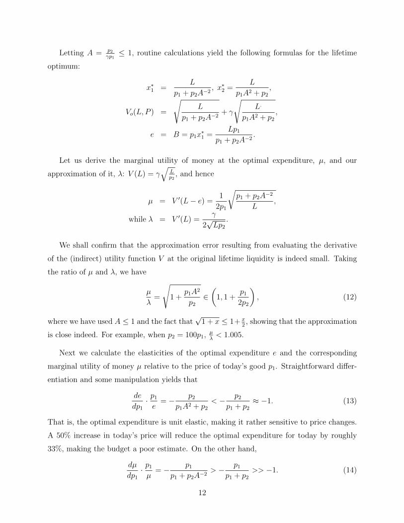
Letting A = p2γp1≤ 1, routine calculations yield the following formulas for the lifetime

optimum:

x∗1 =L

p1 + p2A−2, x∗2 =

L

p1A2 + p2,

Vo(L, P ) =

√L

p1 + p2A−2+ γ

√L.

p1A2 + p2,

e = B = p1x∗1 =

Lp1p1 + p2A−2

.

Let us derive the marginal utility of money at the optimal expenditure, µ, and our

approximation of it, λ: V (L) = γ√

Lp2, and hence

µ = V ′(L− e) =1

2p1

√p1 + p2A−2

L,

while λ = V ′(L) =γ

2√Lp2

.

We shall confirm that the approximation error resulting from evaluating the derivative

of the (indirect) utility function V at the original lifetime liquidity is indeed small. Taking

the ratio of µ and λ, we have

µ

λ=

√1 +

p1A2

p2∈(

1, 1 +p12p2

), (12)

where we have used A ≤ 1 and the fact that√

1 + x ≤ 1+ x2, showing that the approximation

is close indeed. For example, when p2 = 100p1,µλ< 1.005.

Next we calculate the elasticities of the optimal expenditure e and the corresponding

marginal utility of money µ relative to the price of today’s good p1. Straightforward differ-

entiation and some manipulation yields that

de

dp1· p1e

= − p2p1A2 + p2

< − p2p1 + p2

≈ −1. (13)

That is, the optimal expenditure is unit elastic, making it rather sensitive to price changes.

A 50% increase in today’s price will reduce the optimal expenditure for today by roughly

33%, making the budget a poor estimate. On the other hand,

dµ

dp1· p1µ

= − p1p1 + p2A−2

> − p1p1 + p2

>> −1. (14)

12

Returning to the example p2 = 100p1, the elasticity is less than 0.01 (in absolute terms). We

can see that the shadow utility of money is highly inelastic, so as a result of a price surprise µ

hardly changes and thus it is still well approximated by λ – which of course remains constant

as it is determined exclusively by the rest-of-life problem.

Finally it may be worth pointing out that as λ is an underestimate of µ – because V is

concave and we use the Taylor approximation below L – it is a marginally better estimate for

price increases, that yield a decrease in the marginal utility of money, than price decreases.

4 Using λ

Several practical complications arise when choosing consumption via the marginal utility

of money. We will now deal with what we see as the most important complications —

indivisible goods, where a marginal analysis does not directly apply; significant shocks to

lifetime income, including the purchase of big ticket items; using price observations to adapt

λ; and liquidity constraints.

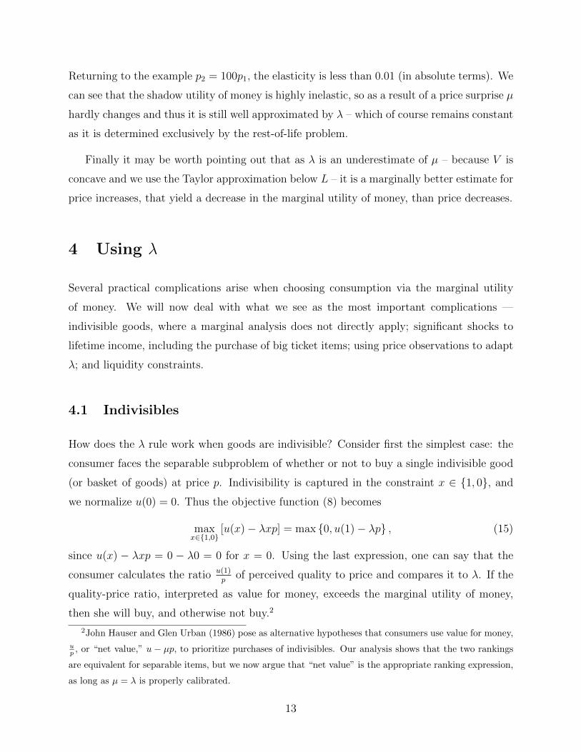
4.1 Indivisibles

How does the λ rule work when goods are indivisible? Consider first the simplest case: the

consumer faces the separable subproblem of whether or not to buy a single indivisible good

(or basket of goods) at price p. Indivisibility is captured in the constraint x ∈ {1, 0}, and

we normalize u(0) = 0. Thus the objective function (8) becomes

maxx∈{1,0}

[u(x)− λxp] = max {0, u(1)− λp} , (15)

since u(x) − λxp = 0 − λ0 = 0 for x = 0. Using the last expression, one can say that the

consumer calculates the ratio u(1)p

of perceived quality to price and compares it to λ. If the

quality-price ratio, interpreted as value for money, exceeds the marginal utility of money,

then she will buy, and otherwise not buy.2

2John Hauser and Glen Urban (1986) pose as alternative hypotheses that consumers use value for money,

up , or “net value,” u − µp, to prioritize purchases of indivisibles. Our analysis shows that the two rankings

are equivalent for separable items, but we now argue that “net value” is the appropriate ranking expression,

as long as µ = λ is properly calibrated.

13

When the consumer has to choose one out of several mutually exclusive varieties or

baskets, the quality-price ratio is no longer sufficient to rank them. A very small basket

may offer a high value for money, but still provide only a small utility gain. Instead, the

consumer ranks baskets bk = (xk1, ..., xkn) of indivisibles (so each xki = 0 or 1) at price vector p

according to their net utility gain, gk = u(bk)−λpbk. She picks the basket with highest gk as

long as it is positive, and otherwise picks the null basket b0 = (0, ..., 0) at price pb0 = 0 and

gain g0 = u(0)− λpb0 = 0. Ignoring trivialities where a more valued basket has lower price,

it follows that basket k will be preferred to basket j if and only if u(bk)−u(bj)pbk−pbj ≥ λ. The gain

in utility by choosing k over j must exceed the shadow utility of the additional expenditure,

i.e., the incremental quality-price ratio must exceed the marginal utility of money.

By contrast, the budget constrained consumer would pick the highest quality item that

does not break her budget. To illustrate the difference, consider the following two scenarios.

In the first, the consumer has two baskets available, with u(b1) < u(b2) and pb1 = B < pb2

while 0 < g2 = u(b2) − λpb2 < u(b1) − λpb1 = g1, so that both decision rules lead to the

purchase of basket 1. The second scenario is the same, except that the price of b2 drops so that

p′b2 = pb1 + ε. According to the budget rule, basket 2 is still not affordable, so the consumer

still buys 1. However, when ε is sufficiently small that g′2 = u(b2)−λp′b2 > u(b1)−λpb1 = g1,

the consumer using the λ rule would switch to the suddenly relatively inexpensive basket.

Crucially, the λ rule would coincide with the new lifetime optimum, while the budget rule

would not.

The appearance of a new variety (or a change in the valuation of an existing one) creates

a similar contrast. Assume that the perceived quality of the expensive option in the first

scenario jumps from u(b2) to a much higher value, with its price remaining constant. This

change would not affect the choice according to the budget rule, but it would clearly lead to

– the lifetime optimal – change in behavior according to the λ rule.

4.2 Adjusting λ

The consumer treats λ as a constant in all subproblems considered so far, but there are

several situations that require an update, even if a full reoptimization of the life-problem is

not necessary.

14

Let us first consider shocks to lifetime income, which are too large to be ignored but not

large enough to necessitate a full reoptimization. In this case the solution is to improve on

the precision of the approximation. The second-order Taylor expansion of the indirect utility

function tells us what is needed. Suppose that lifetime income “jumps” from L0 to L1. The

Taylor approximation around the original lifetime income is V (y) ≈ V (L0)+(y−L0)V′(L0)+

(y−L0)2

2V ′′(L0). We can also approximate V (y) by a first-order Taylor expansion around the

new lifetime income: V (y) ≈ V (L1) + (y − L1)V′(L1). Differentiating both approximations

with respect to y, we have V ′(L0) + (y − L0)V′′(L0) ≈ V ′(L1). Finally, letting y = L1 we

obtain

λ1 = V ′(L1) ≈ V ′(L0) + (L1 − L0)V′′(L0) = λ− β∆L, (16)

where ∆L = L1 − L0 is the change in lifetime income and β = −V ′′(L) ≥ 0 is the rate at

which marginal utility diminishes.

Let us quantify the lifetime income effects that we ignore for small expenditures:

Proposition 3. For two goods, the sensitivity of consumption to lifetime income is given by

dM1(p, λ)

dL≈ −β p1u22 − p2u12

u11u22 − u12u21, (17)

dM2(p, λ)

dL≈ −β p2u11 − p1u21

u11u22 − u12u21, (18)

where all the second partials of u are evaluated at the vector x = M(p, λ).

Of course β is close to zero when V is approximately linear, so these effects are indeed

negligible for small changes of lifetime income. Also note that, just as in the standard model,

it is possible that when her lifetime income increases the consumer buys less of one of the

goods. This is the case of a backward bending IEP (note that the ratio of (17) and (18) gives

us the slope of the IEP), and thus these goods are the same old inferior goods of Marshall.

Proof. We first calculate how the Marshall-Edgeworth demand varies around the optimal

choice as λ changes. Recall from (9) that

u1 (M(p, λ)) = λp1

u2 (M(p, λ)) = λp2.

15

Differentiating both sides of both equations with respect to λ and solving the resulting system

of linear equations we obtain

dM1(p, λ)

dλ=

p1u22 − p2u12u11u22 − u12u21

,

dM2(p, λ)

dλ=

p2u11 − p1u21u11u22 − u12u21

.

Now note that dMi(p,λ)dL

= dMi(p,λ)dλ

· dλdL

. Finally, from (16) we have that dλdL≈ −β and our

proof is complete. Q.E.D.

The purchase of a big ticket item, like an automobile, has a similar effect to a moderate

shock to lifetime income. We can also use a second-order approximation to calculate λ, with

the wealth shock substituted by the representative price of the cars under consideration. In

case the price range considered is so large that the use of the same λ for all varieties leads

to an inaccurate estimate, we can have an individual second order estimate of λ for each

potential item, λi = λ+βpi. The consumer will then choose the variety, bi, which maximizes

her surplus utility u(bi)− λipi.

4.3 Learning the value of money

As the consumer observes more and more prices, she needs to consider updating her λ based

on the new information. We propose a two-step adaptive updating process for λ. The first

step is to translate a price observation into news about the value of λ, and the second is to

determine the magnitude of the update.

Translation is straightforward for indivisible goods. The quality-price ratio u(bk)pbk

is a

natural candidate as a new observation of λ. For divisible goods, we need a somewhat

different procedure – we would never get a new observation, since x is chosen to satisfyu1(x)p1

= λ. Instead, we recall the quantity chosen “last time”, xold, and evaluate the marginal

quality-price ratio at that choice, using the new prices. That is, the new observation of λ isu1(xold)pnew1

.

As for the second step, the logical procedure is to “weight” the new observation according

to its share in overall consumption, the same way as official inflation figures are calculated.3

3Here we assume, for simplicity that the consumer does not try to extrapolate from individual observed

16

In line with the idea that the consumer treats λ as a constant, she will only update it

periodically – say, monthly – in possession of m new observations. Define qi ∈ [0, 1] as the

share of overall expenditure spent on good i in the past “month”. Then the formula to

update λ is

λ′=

(1−

m∑i=1

αiqi

)λ+

m∑i=1

αiqiλi. (19)

Here αi ∈ [0, 1] is the parameter measuring how much the consumer weighs new information

relative to old. It also captures the consumer’s perception of the permanence of any price

changes. Thus a one-off “fire sale” should not carry weight (very low αi) while a price hike

due to a specific tax levied on a product should have an αi close to one.

Other than the permanence of price change issue, we would expect αi not to vary with

categories but to be larger for individuals whose marginal utility diminishes more quickly.

It may be worth noting that when the consumer buys an indivisible good, the new λ

observation will always be above the updated value, while when she does not buy it will

always be below. Thus the decision whether to consume will be the same with the updated

λ as with the old value.

Note that this updating rule also implies that observations of prices of goods that the

consumer does not usually purchase (low qi) do not affect her view of λ. Similarly, if a good

gets priced out of a consumer’s reach, she will stop buying it and this will lead to its exclusion

from effecting her view of λ.

4.4 Saving and borrowing

The budget actually plays two distinct roles that often are conflated in textbook analysis.

So far we have discussed the budget as targeted expenditure (optimal or otherwise) in the

subproblem. The budget also can serve to represent liquidity, a constraint on the purchasing

power available in the subproblem, beyond the lifetime constraint PX = 0 discussed earlier.

This second role can be important even for a new Marshallian consumer, as we will show in

this section.

To deal with liquidity issues, we impose a discrete time structure on lifetime consumption

prices to changes in the price level. See Angus Deaton (1977) for an exploration of that idea.

17

and take the subproblem as single period consumption choice. Thus, for time periods t =

1, 2, ..., let the consumer choose consumption bundle xt ∈ <n+ and receive a net inflow xt0 ∈ <of liquid net income. She earns interest at rate q ≥ −1 on unspent liquid balances, and pays

interest at rate r ≥ q on expenditures in excess of the stock of available liquidity, Lt.4 Thus

the stock of liquidity evolves according to

Lt+1(pxt) = Lt + xt+1

0 − e(pxt, Lt), with e(pxt, Lt) = pxt + r[pxt − Lt

]+ − q [Lt − pxt]+where [y]+ = max{0, y}. That is, tomorrow’s liquidity will be today’s liquidity plus tomor-

row’s liquid income minus today’s net expenditure, e(px, Lt), evaluated tomorrow, including

interest payments.

The indirect utility (or value) function V in (3) now needs to track liquid assets more

carefully. We rewrite it as follows.

Vt(Lt) = maxx≥0

[u(x) + Vt+1 (Lt+1(px))

]. (20)

As a result of the change in the set of feasible consumption paths, the slope V ′t+1 (Lt+1(px)) ,

and thus the marginal utility of money, will be different from V ′t+1(L) in the frictionless case.

Linearizing as before, we have

maxx≥0

[u(x)− λe(px, Lt)]. (21)

The first-order conditions are

ui(x∗) = λpi, i = 1, ..., n, (22)

where

λ =

λ(1 + q), if Lt > px

λ(1 + r), if Lt < px.(23)

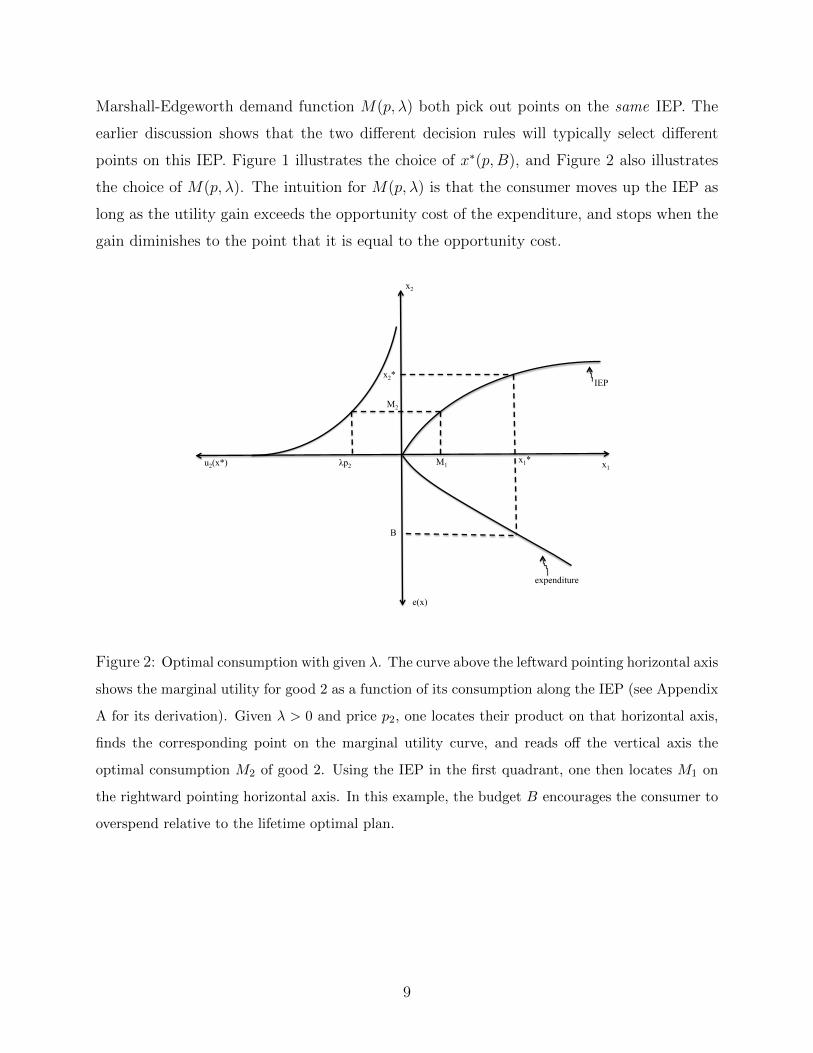
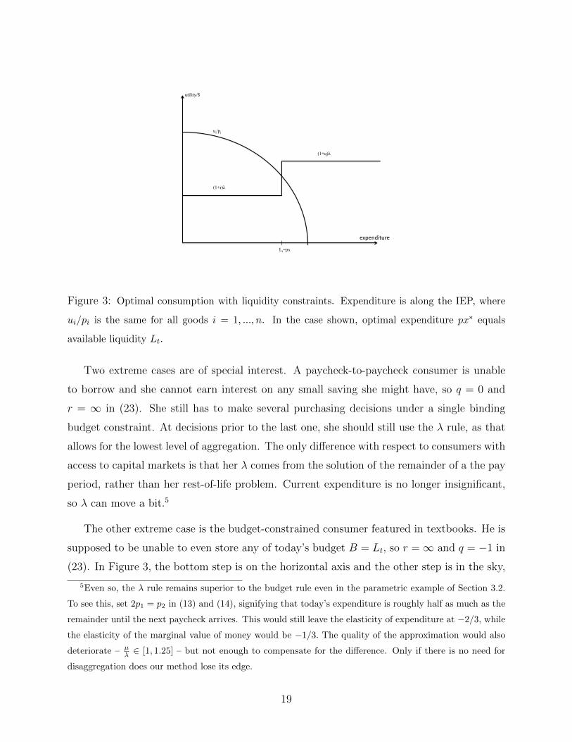
The case r = q is essentially the same as before, after rescaling. When r < q, however,

we have in effect a non-constant λ. Figure 3 shows what then happens in the omitted case

Lt = px in (23).

4We assume constant one-period interest rates, but the reasoning here could be extended to deal with

multi-period interest rates that rise with indebtedness and shift downward when additional collateral (illiquid

assets) are available. This could lead to a strictly increasing λ as opposed to the simple step function of

Figure 3.

18

ui/pi

(1+q)λ

Lt=px

utility/$

(1+r)λ

expenditure  

Figure 3: Optimal consumption with liquidity constraints. Expenditure is along the IEP, where

ui/pi is the same for all goods i = 1, ..., n. In the case shown, optimal expenditure px∗ equals

available liquidity Lt.

Two extreme cases are of special interest. A paycheck-to-paycheck consumer is unable

to borrow and she cannot earn interest on any small saving she might have, so q = 0 and

r = ∞ in (23). She still has to make several purchasing decisions under a single binding

budget constraint. At decisions prior to the last one, she should still use the λ rule, as that

allows for the lowest level of aggregation. The only difference with respect to consumers with

access to capital markets is that her λ comes from the solution of the remainder of a the pay

period, rather than her rest-of-life problem. Current expenditure is no longer insignificant,

so λ can move a bit.5

The other extreme case is the budget-constrained consumer featured in textbooks. He is

supposed to be unable to even store any of today’s budget B = Lt, so r =∞ and q = −1 in

(23). In Figure 3, the bottom step is on the horizontal axis and the other step is in the sky,

5Even so, the λ rule remains superior to the budget rule even in the parametric example of Section 3.2.

To see this, set 2p1 = p2 in (13) and (14), signifying that today’s expenditure is roughly half as much as the

remainder until the next paycheck arrives. This would still leave the elasticity of expenditure at −2/3, while

the elasticity of the marginal value of money would be −1/3. The quality of the approximation would also

deteriorate – µλ ∈ [1, 1.25] – but not enough to compensate for the difference. Only if there is no need for

disaggregation does our method lose its edge.

19

so the consumer always chooses to spend exactly B = Lt.

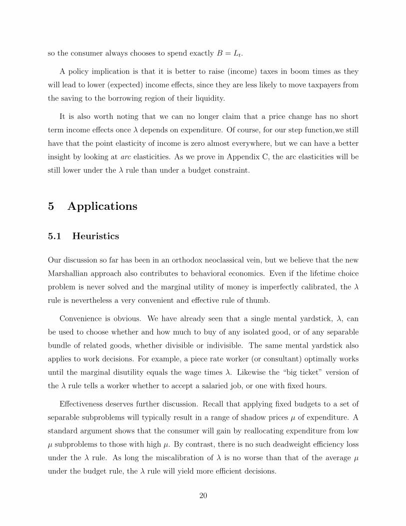
A policy implication is that it is better to raise (income) taxes in boom times as they

will lead to lower (expected) income effects, since they are less likely to move taxpayers from

the saving to the borrowing region of their liquidity.

It is also worth noting that we can no longer claim that a price change has no short

term income effects once λ depends on expenditure. Of course, for our step function,we still

have that the point elasticity of income is zero almost everywhere, but we can have a better

insight by looking at arc elasticities. As we prove in Appendix C, the arc elasticities will be

still lower under the λ rule than under a budget constraint.

5 Applications

5.1 Heuristics

Our discussion so far has been in an orthodox neoclassical vein, but we believe that the new

Marshallian approach also contributes to behavioral economics. Even if the lifetime choice

problem is never solved and the marginal utility of money is imperfectly calibrated, the λ

rule is nevertheless a very convenient and effective rule of thumb.

Convenience is obvious. We have already seen that a single mental yardstick, λ, can

be used to choose whether and how much to buy of any isolated good, or of any separable

bundle of related goods, whether divisible or indivisible. The same mental yardstick also

applies to work decisions. For example, a piece rate worker (or consultant) optimally works

until the marginal disutility equals the wage times λ. Likewise the “big ticket” version of

the λ rule tells a worker whether to accept a salaried job, or one with fixed hours.

Effectiveness deserves further discussion. Recall that applying fixed budgets to a set of

separable subproblems will typically result in a range of shadow prices µ of expenditure. A

standard argument shows that the consumer will gain by reallocating expenditure from low

µ subproblems to those with high µ. By contrast, there is no such deadweight efficiency loss

under the λ rule. As long the miscalibration of λ is no worse than that of the average µ

under the budget rule, the λ rule will yield more efficient decisions.

20

How good an estimate of λ should we expect in typical consumers? Faced with a new

subproblem, the consumer need not try to re-solving her lifetime problem (1) or (3). Instead,

it can be inferred from her work plan. The marginal utility of leisure divided by the wage

is a simple approximation of λ, and it is precisely correct when labor choice is an interior

optimum. Previous consumption decisions, of course, also provide convenient estimates of

λ; a consumer who has taken the trouble to optimize once can subsequently free ride on her

own calculations.

Of course, some consumers may have a persistently biased view of their true marginal

utility for money. A miser is someone who (perhaps because of an impoverished childhood

and stalled adjustment) maintains an unreasonably high λ, relative to typical preferences

and to his actual lifetime opportunities. Likewise a spendthrift maintains an unreasonably

low λ. Thus the λ rule can be thought of as a heuristic, which is suboptimal to the extent

that λ is badly calibrated.

Recent behavioral economics literature includes an alternative heuristic called narrow

bracketing, or mental accounting (e.g., Daniel Read, George Lowenstein and Matthew Rabin,

1999; or Richard Thaler, 1999). In our terminology, the claim is that consumers sometimes

treat non-separable subproblems as if they were separable, resulting in inefficient choices,

especially when self control is problematic. For example, a consumer may regard the health

risk as negligible when considering smoking a single cigarette. The addictive properties of

nicotine warrant a broader definition of the subproblem, and the consumer might come to a

different conclusion when considering smoking a pack a day for a year, or for a decade.

In our view, this literature underlines the importance of separability in defining subprob-

lems. We agree that treating a non-separable subproblem in isolation will typically lead to

suboptimal behavior. Our contribution lies mainly in how to proceed after identifying (up

to a reasonable approximation) a separable subproblem.

The mental accounting branch of the literature suggests that people may choose a par-

ticular budget for each subproblem, e.g., bring exactly $2500 to Las Vegas. (The ubiquitous

presence of cash machines in casinos suggests that this self-control device is less than 100%

successful!) Our recommendation, of course, is instead to make choices according to λ. This

doesn’t solve all self-control issues, but it has the virtue of simplicity. The consumer then

only needs to carry a single number, while a consumer using mental accounting would have

21

to remember a vector. Additionally, we have a simple procedure for how to adapt λ to

persistent price changes, while we know of no such method for budgets, mental or otherwise.

When is each heuristic more commonly used? This seems like a good question to take

to the laboratory, especially since payments received in lab experiments are normally quite

separate from the rest of the subject’s life. One could set up various moderately complicated

lab tasks, and in one treatment frame the tasks in terms of budgets and in another treatment

frame them in terms of the marginal utility of money. Then one could check which treatment

encouraged more efficient choices. A more direct test is simply to provide access to budgeting

tools as well as λ-oriented tools, and to see which the subjects prefer to use.6

5.2 Disaggregated decisions in firms

Multidivisional firms face a question reminiscent of ours: under what conditions can the

firm profitably decentralize real investment decisions? To the extent that the divisions are

separable, the new Marshallian approach suggests the following decentralized procedure. Let

λ be the parent firm’s opportunity cost of funds, typically proxied by the weighted average

cost of capital. Then each division should invest in scalable projects up to the point that

the marginal return falls to λ, and choose among mutually exclusive projects by maximizing

present value calculated using λ, the direct generalization of the g rule in section 4.1. When

divisions are not separable, the returns should be estimated in terms of incremental net

benefit to the firm as a whole, rather than just to the division. Remarkably, this procedure

is essentially the same as that recommended in standard corporate finance textbooks (see,

for example, Steven Ross, Randolph Westerfield and Bradford Jordan, 2008, Part Four).

Martin Weitzman (1974) discusses the decentralization of decisions on the production

side. He compares the relative advantages of quantity targets vs. transfer prices for a

production unit that is subject to frequent shocks to its costs. He finds no clear winner as

the dead-weight losses depend on the relative slopes of marginal cost and marginal benefit

curves (much like the incidence of ad valorem taxes).7 Weitzman agrees with us when he

6We are grateful to Ryan Oprea for suggesting this line of inquiry.7The new Marshallian approach would fit into this framework by interpreting λ as the (constant) marginal

benefit from the production of an additional unit. For such a situation Weitzman would declare transfer

price, that is λ, as the clear winner.

22

concludes that prices have a comparative advantage when coordination between units is not

a major concern and when there are several units producing substitutes .

5.3 Money illusion

Of course, lifetime utility U(X) depends only on actual work and consumption, and is

independent of nominal quantities such as L and P . Indeed, the indirect utility function

is homogeneous of degree 0 in (L, P ) (see, for example, Varian (1992), p. 102). Hence a

proportional change in all prices (and wages) will have no effect on the work/consumption

plans or utility of Homo Economicus. The same is true in the textbook consumer choice

subproblem with the budget B adjusted in the same proportion as the price vector.

However, inflation in the real world is much messier than a simultaneous proportional

change. An important empirical regularity is that relative prices become more volatile as the

measured rate of inflation rises (see, for example, Daniel Heymann and Axel Leijonhufvud,

1995). Actual people updating λ, therefore, are unlikely to immediately adjust to a change

in the price level. According to (19) they will overreact to nominal increases in wages and

lag in reacting to observed nominal increases in prices of purchased goods (see, for example,

David Genesove and Christopher Mayer, 2001). That is, in the parlance of macroeconomic

theory, they will suffer from money illusion.

Eventually, however, they should adapt fully to the new price level. For a proportional

upward change in all prices (and wages, etc.) from P to cP , with c > 1, then λ will shift

downward proportionately to λ/c.8 Money is worth less at a higher price level.

6 Discussion

The new Marshallian approach to consumer choice centers on λ, the marginal utility of

money. It applies to any separable subproblem regarding work, or consumption, or both,

and λ can be described as the opportunity cost of expenditure in the continuation game

8This can be seen from the general result that derivatives of homogeneous degree k functions are

homogeneous degree k − 1, or verified directly from the definitions: λ′ = limch→0V (cL−ch)−V (cL)

ch =

c−1 V (L−h)−V (L)h = c−1λ. The middle equality follows from the degree 0 homogeneity of V .

23

following the subproblem. The λ rule states that expenditure on a good (or on the efficient

bundles of goods along an appropriate income expansion path, IEP) should increase until

its marginal utility diminishes to λ.

The resulting Marshall-Edgeworth demand functions M(p, λ) share some features with

their standard and Hicksian counterparts x∗(p,B) and h(p, u) – notably, for a given subprob-

lem price vector p, all three lie on the same IEP – but M has several distinct advantages.

• It is very simple and specific – the single number λ is a sufficient statistic for the hugely

complex rest-of-life problem. By contrast, each subproblem requires its own budget B

in the standard approach, and short of re-solving the lifetime problem, it is unclear

how B might be determined.

• It is robust to changes in subproblem prices. No change in λ is required when p changes.

By contrast, the appropriate B depends sensitively on p.

• Its elasticities are a first-order approximation of the true General Equilibrium elastici-

ties, and the approximation is exact in a fully separable subproblem whose expenditure

is a negligible part of lifetime income. Standard or Hicksian elasticities are close to GE

elasticities in such subproblems only in the special case that they coincide with M ’s.

• It is quite intuitive – the consumer tries directly to get her money’s worth. We suspect

that it is also quite descriptive of actual consumer behavior, but we are not aware of

any empirical studies so far that compare the predictive power of M and x∗.

To better understand the new Marshallian approach, recall the traditional distinction

between non-pecuniary consumption externalities and pecuniary externalities. The first kind

recognizes that how much the consumer values a certain quantity of a good may depend on

what else is in her consumption basket. Often this kind of externality extends only to a small

set of goods, e.g., a few complements and close substitutes, and then we can internalize this

externality in a tractable separable subproblem of the lifetime problem. The second kind,

pecuniary externalities, are pervasive and not so easy to encapsulate. Expenditures are

mutually exclusive, and money spent on one good is not available to purchase any other

good. But λ precisely captures this kind of externality.

24

By contrast, it is hard to specify the appropriate subproblem to which to apply a budget

B in the standard approach. The larger the set of goods, the better internalized is the

pecuniary externality, and the closer one gets to the true lifetime GE problem. But at the

same time, one loses the tractability of low-dimensional partial equilibrium analysis.

The new approach points up the fact that partial equilibrium analysis routinely conflates

the available liquidity L with the expenditure B targeted at a subproblem. Otherwise put,

the natural subproblem boundaries need not coincide with the boundaries of binding liquidity

constraints. Given access to perfectly liquid financial markets, it is erroneous to specify B

other than the lifetime budget constraint. When there are additional liquidity constraints,

they are best dealt with as in section 4.4, where the textbook analysis is shown to be an

extreme and unrealistic special case.

Some readers may object to our use of cardinal utility functions. But the insistence on

ordinal utility for consumer choice seems increasingly anomalous, since cardinal utility has

become so pervasive elsewhere in economics. Varian’s textbook, for example, uses cardinal

functions without apology in earlier chapters on production technology and later chapters

on risky choice. Why should the sole exception be consumer choice in the absence of risk?

A key insight from the new Marshallian approach is that budgets should not be applied

piecemeal to subproblems, but instead all subproblems should be solved consistently using a

single sufficient statistic, the marginal utility of money. The point is that funds are fungible,

as has long been recognized in other branches of economics.9

One final thought. For several generations, economics instructors have tortured under-

graduates with various decompositions of income and substitution effects, and picky dis-

tinctions between gross and net substitutes and complements, etc. One benefit of the new

Marshallian approach is that it will sweep away such dross, and restore a measure of common

sense to consumer choice theory.

9In public finance, for example, it is well known that a uniform income tax is more efficient for raising a

given amount of revenue than a collection of specific taxes on individual items. We thank Donald Wittman

for pointing out the analogy.

25

7 Notes on related literature

Following the initial intellectual boost by Friedrich Hayek (1945), the issue of partial ag-

gregation was the subject of a lot of (very technical) study more than half a century ago.

The idea was to find (nearly) separable parts of an economic problem so that the external-

ities across parts can be internalized in a manageable manner. Main contributions include

Wassily Leontieff (1947), Robert Strotz (1957, 1959), Terence Gorman (1959, 1968), Herbert

Simon and Albert Ando (1961), and Gerard Debreu (1960). The latter offers an ordinal

definition of separability, essentially that preferences over x, y ∈ ξ[n] are independent of X⊥.

He shows under quite general conditions that this entails a cardinal (vNM) utility function

over separable subproblems.10

While we also feel inspired by Hayek, our contribution is more conceptual than this

literature and does not delve into the technicalities of separability/aggregation more than

strictly necessary to get our ideas across.

James C. Cox (1975) provides a more complete derivation of the indirect utility function

than we do, though with an emphasis on financial assets.

Xavier Vives (1987) has a kindred contribution to ours in that he also attempts to bring

Marshallian ideas back to the mainstream and use them to defend the partial equilibrium

approach. He shows that as the number of goods, n, increases, the income effects in any

single market are indeed vanishing at at least a rate of 1/√n.

Finally, Jozsef Sakovics (2011) was the first to present a model of consumer choice where

budget constraints are soft. In his case the consumers misperceive prices and hence satisfy

the budget constraint for these, so actually they either under or overspend.

10Our thanks to Luciano Andreozzi for bringing this paper to our attention.

26

8 Appendix

8.1 Appendix A: Marginal utility along the IEP

Let x∗1(x2) denote the IEP. We know that

p2u1 (x∗1(x2), x2) ≡ p1u2 (x∗1(x2), x2) .

Differentiating both sides according to x2 we obtain

p2

(dx∗1(x2)

dx2u11 + u12

)= p1

(dx∗1(x2)

dx2u21 + u22

),

which simplifies todx∗1(x2)

dx2=p2u12 − p1u22p1u21 − p2u11

,

giving us the slope of the IEP.

Now we can derive the formula for the marginal utility of good 2 along the IEP:

du (x∗1(x2), x2)

dx2=dx∗1(x2)

dx2u1 + u2 =

p2u12 − p1u22p1u21 − p2u11

u1 + u2.

8.2 Appendix B: Decomposition of price effects

The textbook price effects are ordinal, shaped by the budget constraint, and involve the

Slutsky decomposition into substitution and income effects. The standard Sltutsky equation

is∂xi(p, e)

∂p1=∂hi(p, u(p, e))

∂p1− xi(p, e)

∂xi(p, e)

∂e, (24)

where x(p, e) is the standard demand at prices p and available expenditure e, and h(p, u)

denotes the Hicksian (expenditure minimizing) demand at prices p and achieved utility u.

The first right hand term in (24) is the substitution effect, measuring the rate of movement

along a fixed indifference curve onto a new IEP as a result of a price change. The second

term is the income effect, the sign of which depends on the slope of the Engel curve, ∂xi(p,e)∂e

.

27

The new Marshallian counterpart of (24) can be obtained by differentiating both sides of

the identity Mi(p, λ) ≡ xi(p, e(p, λ)), where e(p, λ) is the optimal expenditure given p and λ.

∂Mi(p, λ)

∂p1=∂xi(p, e)

∂p1+∂xi(p, e)

∂e· ∂e(p, λ)

∂p1(25)

Substituting (24) into (25) one obtains

∂Mi(p, λ)

∂p1=∂hi(p, u(p, e))

∂p1+∂xi(p, e)

∂e·(∂e(p, λ)

∂p1− xi(p, e)

). (26)

Equation (26) shows that the substitution effect is the same in both models. This comes

as no surprise, as the substitution effect only depends on the new IEP, which – as we have

seen – is model independent. The remaining term, which we shall call the expenditure effect,

is quite different from its textbook counterpart. Instead of arising from an effort to keep

nominal expenditure constant as prices change (as in the textbook analysis), it comes from

adjusting expenditure for a given marginal utility of money.

Proposition 4. The difference between the income and the expenditure effects is

D = −[x1(p, e) +

(p1∂M1(p, λ)

∂p1+ p2

∂M2(p, λ)

∂p1

)]∂xi(p, e)

∂e. (27)

Proof. Subtract (26) from (24) to obtain the difference is −∂e(p,λ)∂p1

· ∂xi(p,e)∂e

. By definition

e(p, λ) = M1(p, λ)p1 +M2(p, λ)p2, and differentiating that identity wrt p1 yields

∂e(p, λ)

∂p1= M1(p, λ) + p1

∂M1(p, λ)

∂p1+ p2

∂M2(p, λ)

∂p1.

The consumption of the first good can be written M1(p, λ) = x1(p, e), so we obtain the

desired expression. Q.E.D.

The interpretation of (27) is the following. When a consumer is constrained by a budget,

the sensitivity of her expenditure to p1 (holding utility constant) is

∂e(p, u)

∂p1= h1(p, u) + p1

∂h1(p, u)

∂p1+ p2

∂h2(p, u)

∂p1= h1(p, u) = x1(p, e),

where the last two terms add to zero by the standard tangency condition at the optimum:

−p1p2

= ∂h2(p,u)∂h1(p,u)

. In other words, as the consumer must keep spending the same amount,

the price change has an income effect proportional to the pre-change consumption of the

good. When the consumer can freely move purchasing power across the boundary of the

28

subproblem, the expenditure changes in line with the new demand, taking into account the

optimal adjustment of consumption.

The following corollary is immediate:

Corollary 1. Either own or cross price elasticity of demand is larger in the new Marshallian

model than in the standard one if and only if either the good in question is normal and

M1 >u2u21−u1u22u11u22−u12u21 , or the good is inferior and M1 <

u2u21−u1u22u11u22−u12u21 .

Proof. We use Proposition 2 together with the identity λpi = ui, to obtain that D =[−M1 − u1u22−u2u21

u11u22−u12u21

]∂xi(p,e)∂e

. Q.E.D.

8.3 Appendix C: Income elasticity with liquidity constraints

Proposition 5. For normal goods, the (short term) income arc elasticity of demand is

strictly lower when the consumer is not budget constrained, but uses the λ rule.

Proof. Without loss of generality, let us assume that the income shock is positive, denote

it by ∆. In that case, the effect on λ will be non-positive – as by normality all the marginal

utility functions will shift down – and it will be negative only if the consumer moves from

borrowing to saving.11 If she borrowed before then µ(B) > λ(1 + r), if she is saving now

then µ(B + ∆) < λ(1 + q), implying that µ(B) − µ(B + ∆) > λ(r − q). As the changes in

marginal utility are proportional to the changes in the Lagrange multipliers (c.f. (6)), the

proof is complete. Q.E.D.

It is worth noting that an implication of Proposition 5 is that by allowing for the smooth-

ing of income shocks across periods our model makes the current consumption decisions less

responsive to these shocks, providing a possible a micro-foundation for the Permanent Income

Hypothesis in a disaggregated environment.

11In the case that the consumer spends her liquidity exactly, we can impute her a λ ∈ [λ(1 + q), λ(1 + r)],

and the same argument goes through (c.f. Figure 3).

29

References

[1] Bentham, J. (1802) Theory of legislation. Edited by E. Dumont, translated from the

original French by C.M. Atkinson in 1914. Oxford University Press.

[2] Cox, J.C. (1975) “Portfolio Choice and Saving in an Optimal Consumption-Leisure

Plan,” Review of Economic Studies, XLII(1), 105-116.

[3] Deaton, A. (1977) “Involuntary Saving Through Unanticipated Inflation,” American

Economic Review, 67(5), 899-910.

[4] Debreu G. (1960) “Topological Methods in Cardinal Utility Theory,” in Arrow, Karlin

and Suppes, editors, Mathematical Methods in the Social Sciences.

[5] Genesove, D. and Mayer, C. (2001) “Loss Aversion and Seller Behavior: Evidence from

the Housing Market,” Quarterly Journal of Economics, 116(4), 1233-1260.

[6] Gorman, W.M. (1959) “Separable Utility and Aggregation,” Econometrica, 27(3), 469-

481.

[7] Gorman, W.M. (1968) “Conditions for Additive Separability,” Econometrica, 36(3/4),

605-609.

[8] Hauser, J.R. and Urban, G.L. (1986) “The Value Priority Hypotheses for Consumer

Budget Plans” Journal of Consumer Research, 12(4), 446-462.

[9] Hayek, F.A. (1945) “The Use of Knowledge in Society,” American Economic Review,

35(4), 519–530.

[10] Heymann, D. and Leijonhufvud, A. (1995) High Inflation, The Arne Ryde Memorial

Lectures, Oxford University Press.

[11] Hicks, J.R. and Allen, R.G.D. (1934) “A Reconsideration of the Theory of Value,”

Economica, Part I: 1(1), 52-76; Part II: 1(2), 196-219.

[12] Leontieff, W. (1947) “Introduction to a Theory of the Internal Structure

of Functional Relationships,” Econometrica, 15(4), 361-373.

30

[13] Marshall, A. (1890/1920) Principles of economics. London: Macmillan.

[14] Read, D., Lowenstein, G. and Rabin, M. (1999) “Choice bracketing,” Journal of Risk

and Uncertainty, 19(1-3),171-197.

[15] Ross, S.A., Westerfield, R.W and Jordan, B.D., (2008), Fundamentals of Corporate

Finance, 8th Edition, McGraw-Hill.

[16] Sakovics, J. (2011) “Reference Distorted Prices,” Quantitative Marketing and Eco-

nomics, forthcoming, available on-line.

[17] Simon, H. A. and Ando, A. (1961) “Aggregation of Variables in Dynamic Systems,”

Econometrica, 29(2), 111-138.

[18] Stigler, G. J. (1950) “The Development of Utility Theory. I,” Journal of Political Econ-

omy, 58, 307-27.

[19] Strotz, R.H. (1957) “The Empirical Implications of a Utility Tree,” Econometrica, 25(2),

269-280.

[20] Strotz, R.H. (1959) “The Utility Tree–A Correction and Further Appraisal,” Economet-

rica, 27(3), 482-488.

[21] Thaler, R.H. (1999) “Mental Accounting Matters,” Journal of Behavioral Decision Mak-

ing, 12(3), 183-206.

[22] Varian, H.R. (1992) Microeconomic Analysis, Third Edition, W.W. Norton and Co.,

New York.

[23] Vives, X. (1987) “Small Income Effects: A Marshallian Theory of Consumer Surplus

and Downward Sloping Demand,” Review of Economic Studies, 54, 87-103.

[24] Weitzman, M.L. (1974) “Prices vs. Quantities,” Review of Economic Studies, 41(4),

477-491.

31