The Convolution Sum for DT LTI Systems

The Convolution Sum for Discrete-Time LTI Systems

Andrew W. H. House

01 June 2004

1 The Basics of the Convolution Sum

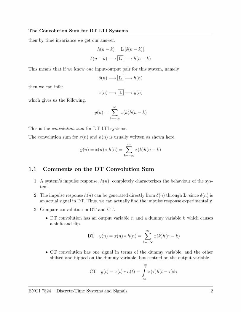
Consider a DT LTI system, L.

x(n) −→ L −→ y(n)

DT convolution is based on an earlier result where we showed that any signal x(n) can beexpressed as a sum of impulses.

x(n) =∞∑

k=−∞

x(k)δ(n− k)

So let us consider x(n) written in this form to be our input to the LTI system.

y(n) = L [x(n)] = L

[∞∑

k=−∞

x(k)δ(n− k)

]

This looks like our general linear form with a scalar x(k) and a signal in n, δ(n− k). Recallthat for an LTI system:

• Linearity (L): ax1(n) + bx2(n) −→ L −→ ay1(n) + by2(n)

• Time Invariance (TI): x(n− no) −→ L −→ y(n− no)

We can use the property of linearity to distribute the system L over our input.

y(n) = L

[∞∑

k=−∞

x(k)δ(n− k)

]=

∞∑k=−∞

x(k)L [δ(n− k)]

So now we wonder, what is L [δ(n− k)]? Well, we can figure it out. Suppose we know howL acts on one impulse δ(n), and we call it

h(n) = L [δ(n)]

ENGI 7824 – Discrete-Time Systems and Signals 1

The Convolution Sum for DT LTI Systems

then by time invariance we get our answer.

h(n− k) = L [δ(n− k)]

δ(n− k) −→ L −→ h(n− k)

This means that if we know one input-output pair for this system, namely

δ(n) −→ L −→ h(n)

then we can inferx(n) −→ L −→ y(n)

which gives us the following.

y(n) =∞∑

k=−∞

x(k)h(n− k)

This is the convolution sum for DT LTI systems.

The convolution sum for x(n) and h(n) is usually written as shown here.

y(n) = x(n) ∗ h(n) =∞∑

k=−∞

x(k)h(n− k)

1.1 Comments on the DT Convolution Sum

1. A system’s impulse response, h(n), completely characterizes the behaviour of the sys-tem.

2. The impulse response h(n) can be generated directly from δ(n) through L, since δ(n) isan actual signal in DT. Thus, we can actually find the impulse response experimentally.

3. Compare convolution in DT and CT.

• DT convolution has an output variable n and a dummy variable k which causesa shift and flip.

DT y(n) = x(n) ∗ h(n) =∞∑

k=−∞

x(k)h(n− k)

• CT convolution has one signal in terms of the dummy variable, and the othershifted and flipped on the dummy variable, but centred on the output variable.

CT y(t) = x(t) ∗ h(t) =

∞∫−∞

x(τ)h(t− τ)dτ

ENGI 7824 – Discrete-Time Systems and Signals 2

The Convolution Sum for DT LTI Systems

4. CT convolution is a model of behaviour of CT systems.

DT convolution is a model of behaviour of DT systems, but also an algorithm we canuse to implement the system, since it is computable. This is another reason why weprefer DT signals and systems.

2 Examples of Convolution

Convolution is best understood when seen in action. Let’s look at a couple of examples,one using signals and impulse responses defined functionally, and another with an impulseresponse defined point-wise.

Example 2.1: DT Convolution: Step Response

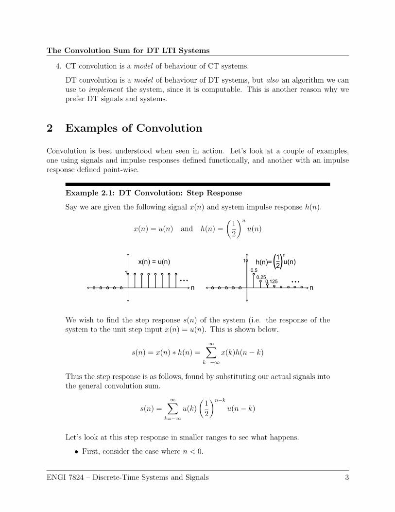
Say we are given the following signal x(n) and system impulse response h(n).

x(n) = u(n) and h(n) =

(1

2

)n

u(n)

We wish to find the step response s(n) of the system (i.e. the response of thesystem to the unit step input x(n) = u(n). This is shown below.

s(n) = x(n) ∗ h(n) =∞∑

k=−∞

x(k)h(n− k)

Thus the step response is as follows, found by substituting our actual signals intothe general convolution sum.

s(n) =∞∑

k=−∞

u(k)

(1

2

)n−k

u(n− k)

Let’s look at this step response in smaller ranges to see what happens.

• First, consider the case where n < 0.

ENGI 7824 – Discrete-Time Systems and Signals 3

The Convolution Sum for DT LTI Systems

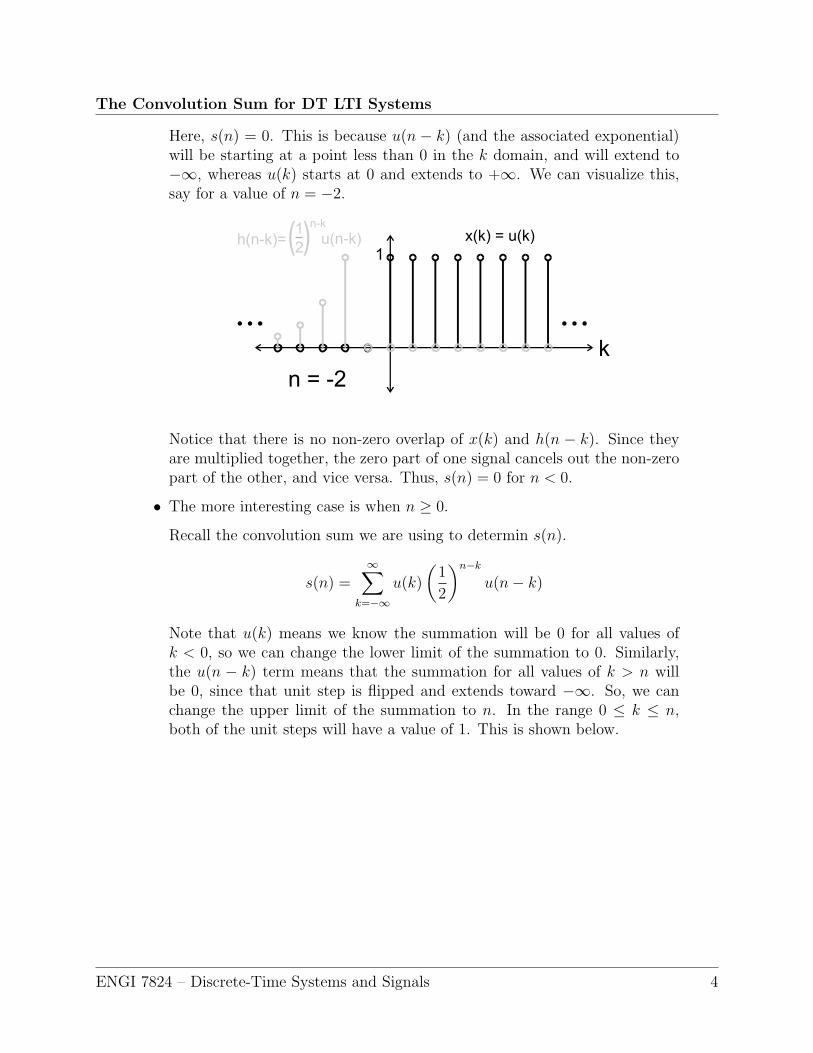
Here, s(n) = 0. This is because u(n − k) (and the associated exponential)will be starting at a point less than 0 in the k domain, and will extend to−∞, whereas u(k) starts at 0 and extends to +∞. We can visualize this,say for a value of n = −2.

Notice that there is no non-zero overlap of x(k) and h(n − k). Since theyare multiplied together, the zero part of one signal cancels out the non-zeropart of the other, and vice versa. Thus, s(n) = 0 for n < 0.

• The more interesting case is when n ≥ 0.

Recall the convolution sum we are using to determin s(n).

s(n) =∞∑

k=−∞

u(k)

(1

2

)n−k

u(n− k)

Note that u(k) means we know the summation will be 0 for all values ofk < 0, so we can change the lower limit of the summation to 0. Similarly,the u(n − k) term means that the summation for all values of k > n willbe 0, since that unit step is flipped and extends toward −∞. So, we canchange the upper limit of the summation to n. In the range 0 ≤ k ≤ n,both of the unit steps will have a value of 1. This is shown below.

ENGI 7824 – Discrete-Time Systems and Signals 4

The Convolution Sum for DT LTI Systems

s(n) =∞∑

k=−∞

u(k)

(1

2

)n−k

u(n− k)

=n∑

k=0

1 ·(

1

2

)n−k

· 1

We can pull out any terms only in n

since that is not the summation variable.

=n∑

k=0

(1

2

)n(1

2

)−k

=

(1

2

)n n∑k=0

(1

2

)−k

=

(1

2

)n n∑k=0

2k

Now we have a form consistent with a geometric series. We can use that tosolve.

Recalln∑

k=0

2k =1− 2n+1

1− 2= 2n+1 − 1

So we have s(n) as follows.

s(n) =

(1

2

)n (2n+1 − 1

)=

(1

2

)n

(2 · 2n − 1)

=

(1

2

)n(

2 ·(

1

2

)−n

− 1

)

= 2 ·(

1

2

)−n(1

2

)n

− 1 ·(

1

2

)n

s(n) = 2−(

1

2

)n

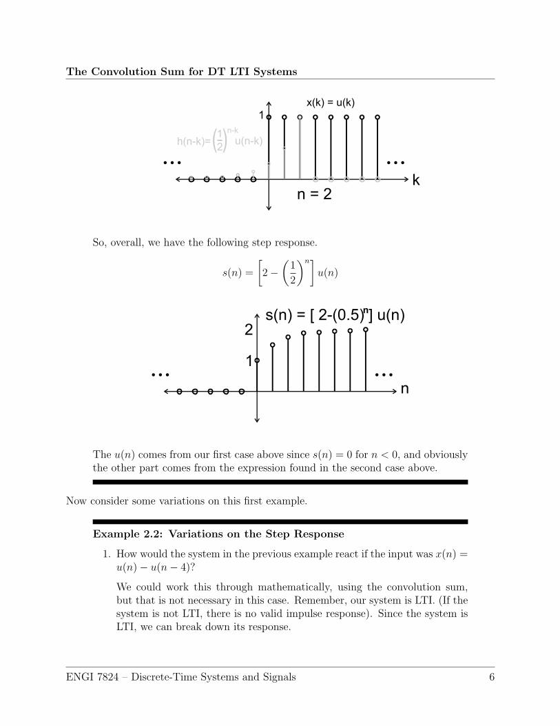
We can visualize this, say for n = 2, as shown below. Note how the systemoutput comes from the overlap of the input signal and the shifted and flippedimpulse response.

ENGI 7824 – Discrete-Time Systems and Signals 5

The Convolution Sum for DT LTI Systems

So, overall, we have the following step response.

s(n) =

[2−

(1

2

)n]u(n)

The u(n) comes from our first case above since s(n) = 0 for n < 0, and obviouslythe other part comes from the expression found in the second case above.

Now consider some variations on this first example.

Example 2.2: Variations on the Step Response

1. How would the system in the previous example react if the input was x(n) =u(n)− u(n− 4)?

We could work this through mathematically, using the convolution sum,but that is not necessary in this case. Remember, our system is LTI. (If thesystem is not LTI, there is no valid impulse response). Since the system isLTI, we can break down its response.

ENGI 7824 – Discrete-Time Systems and Signals 6

The Convolution Sum for DT LTI Systems

y(n) = L[x(n)]

= L[u(n)− u(n− 4)]

= L[u(n)]− L[u(n− 4)]

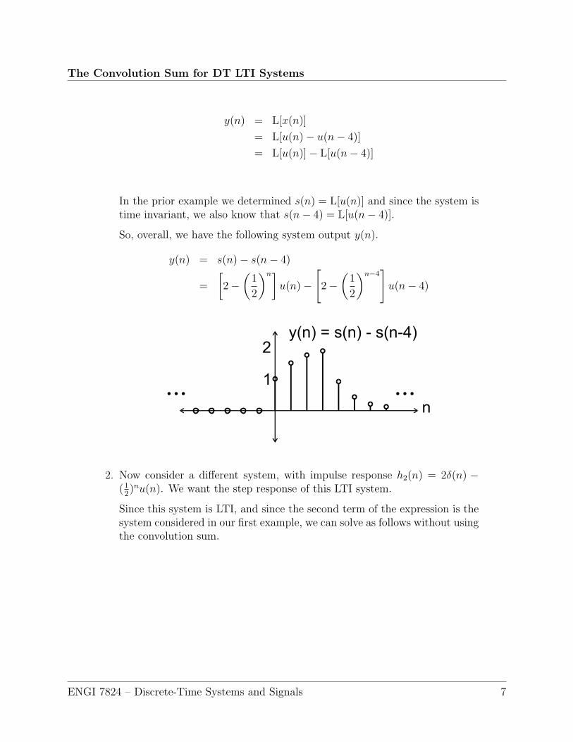
In the prior example we determined s(n) = L[u(n)] and since the system istime invariant, we also know that s(n− 4) = L[u(n− 4)].

So, overall, we have the following system output y(n).

y(n) = s(n)− s(n− 4)

=

[2−

(1

2

)n]u(n)−

[2−

(1

2

)n−4]

u(n− 4)

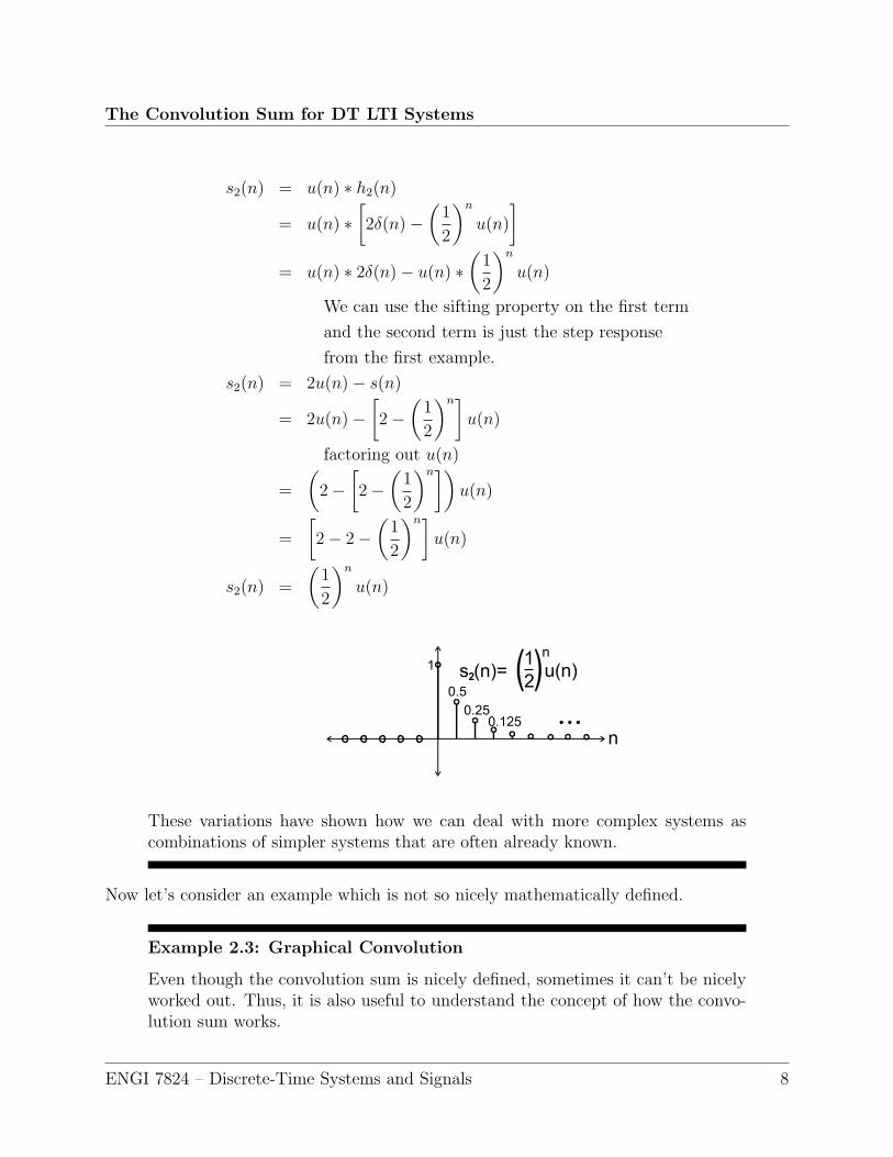
2. Now consider a different system, with impulse response h2(n) = 2δ(n) −(1

2)nu(n). We want the step response of this LTI system.

Since this system is LTI, and since the second term of the expression is thesystem considered in our first example, we can solve as follows without usingthe convolution sum.

ENGI 7824 – Discrete-Time Systems and Signals 7

The Convolution Sum for DT LTI Systems

s2(n) = u(n) ∗ h2(n)

= u(n) ∗[2δ(n)−

(1

2

)n

u(n)

]= u(n) ∗ 2δ(n)− u(n) ∗

(1

2

)n

u(n)

We can use the sifting property on the first term

and the second term is just the step response

from the first example.

s2(n) = 2u(n)− s(n)

= 2u(n)−[2−

(1

2

)n]u(n)

factoring out u(n)

=

(2−

[2−

(1

2

)n])u(n)

=

[2− 2−

(1

2

)n]u(n)

s2(n) =

(1

2

)n

u(n)

These variations have shown how we can deal with more complex systems ascombinations of simpler systems that are often already known.

Now let’s consider an example which is not so nicely mathematically defined.

Example 2.3: Graphical Convolution

Even though the convolution sum is nicely defined, sometimes it can’t be nicelyworked out. Thus, it is also useful to understand the concept of how the convo-lution sum works.

ENGI 7824 – Discrete-Time Systems and Signals 8

The Convolution Sum for DT LTI Systems

In the convolution sum, the impulse response is written as h(n−k), meaning thatin the k domain, the impulse response is shifted by n and flipped around thatpoint. We can visualize the convolution operation as that shifted-and-flippedimpulse response sliding along the k axis from −∞ to ∞ as the summationoccurs. Whenever there is some non-zero overlap between this shifted-and-flippedimpulse response and the input signal, the system output will be non-zero (unlessthe non-zero overlaps cancel each other).

Let’s consider a specific example.

We are given the impulse response shown below.

h(n) =

0 for n < 01 for 0 ≤ n ≤ 3−2 for 4 ≤ n ≤ 50 for n > 5

Let x(n) = u(n− 4).

ENGI 7824 – Discrete-Time Systems and Signals 9

The Convolution Sum for DT LTI Systems

We want to determine

y(n) = x(n) ∗ h(n) =∞∑

k=−∞

x(k)h(n− k)

=∞∑

k=−∞

u(k − 4)h(n− k)

We can use u(k − 4) to change the summation

limits, but it doesn’t help much.

=∞∑

k=4

1 · h(n− k)

but we have no convenient functional representation of h(n) to allow us to solve.

Consider the solution in a piece-wise fashion.

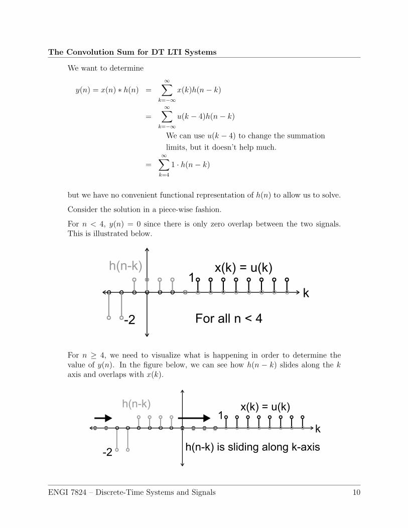
For n < 4, y(n) = 0 since there is only zero overlap between the two signals.This is illustrated below.

For n ≥ 4, we need to visualize what is happening in order to determine thevalue of y(n). In the figure below, we can see how h(n − k) slides along the kaxis and overlaps with x(k).

ENGI 7824 – Discrete-Time Systems and Signals 10

The Convolution Sum for DT LTI Systems

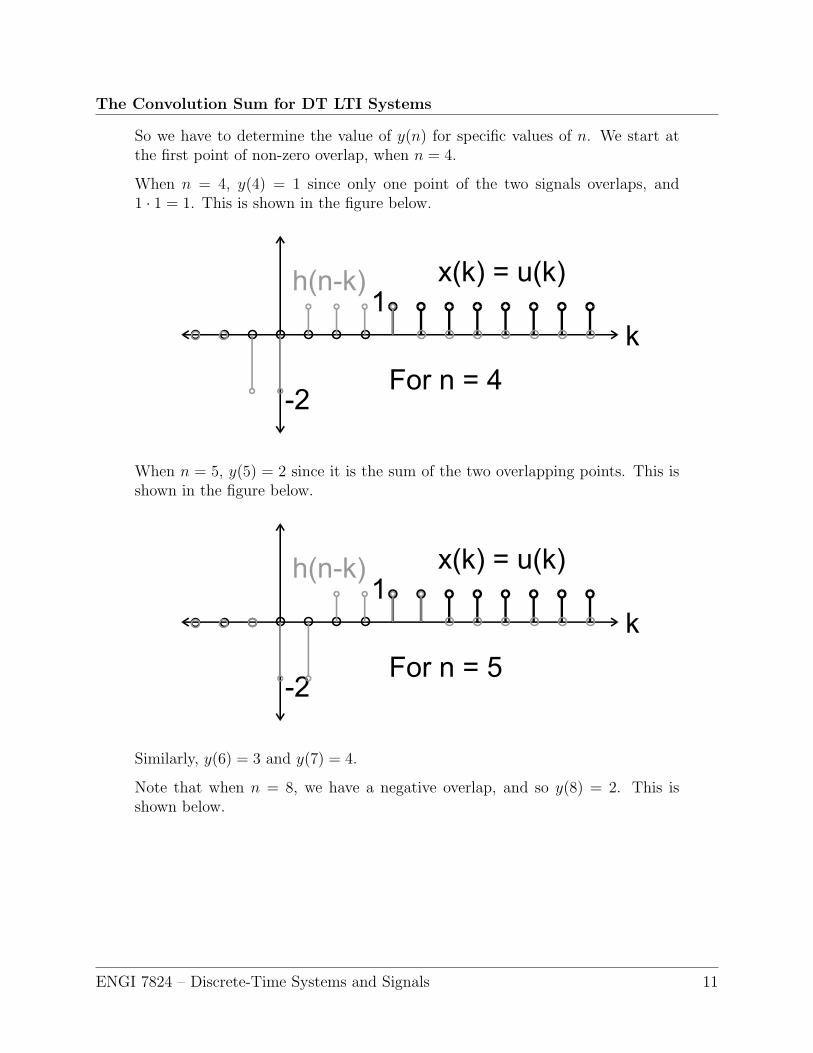
So we have to determine the value of y(n) for specific values of n. We start atthe first point of non-zero overlap, when n = 4.

When n = 4, y(4) = 1 since only one point of the two signals overlaps, and1 · 1 = 1. This is shown in the figure below.

When n = 5, y(5) = 2 since it is the sum of the two overlapping points. This isshown in the figure below.

Similarly, y(6) = 3 and y(7) = 4.

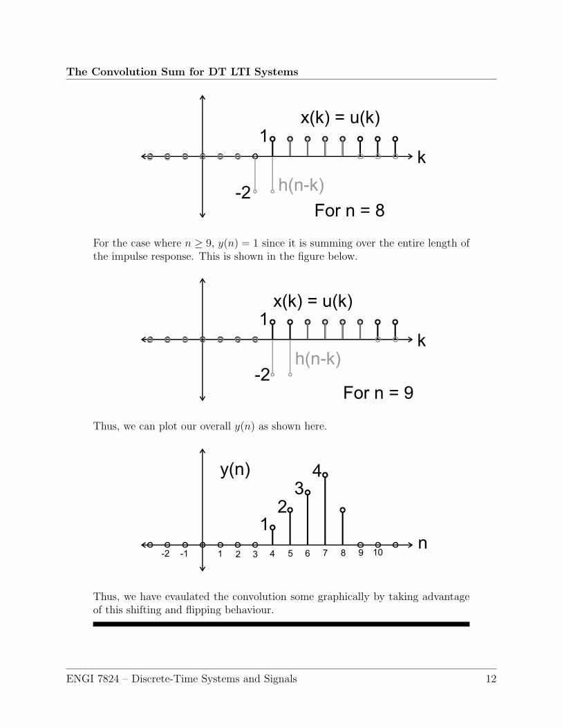
Note that when n = 8, we have a negative overlap, and so y(8) = 2. This isshown below.

ENGI 7824 – Discrete-Time Systems and Signals 11

The Convolution Sum for DT LTI Systems

For the case where n ≥ 9, y(n) = 1 since it is summing over the entire length ofthe impulse response. This is shown in the figure below.

Thus, we can plot our overall y(n) as shown here.

Thus, we have evaulated the convolution some graphically by taking advantageof this shifting and flipping behaviour.

ENGI 7824 – Discrete-Time Systems and Signals 12

The Convolution Sum for DT LTI Systems

3 Basic Properties of DT Convolution

Discrete-time convolution has several useful properties that allows us to solve systems moreeasily.

3.1 Commutativity

Convolution is a commutative operation, meaning signals can be convolved in any order.

x(n) ∗ h(n) = h(n) ∗ x(n)

This quite naturally is true of the convolution sums themselves, as well.

∞∑k=−∞

x(k)h(n− k) =∞∑

k=−∞

h(k)x(n− k)

3.2 Associativity

Convolution is associative, meaning that convolution operations in series can be done in anyorder.

(x(n) ∗ h(n)) ∗ g(n) = x(n) ∗ (h(n) ∗ g(n))

This is significant because it means systems in series can be reordered.

Thus we havex(n) −→ h(n) −→ g(n) −→ y(n)

is the same asx(n) −→ h(n) ∗ g(n) −→ y(n)

is the same asx(n) −→ g(n) ∗ h(n) −→ y(n)

is the same asx(n) −→ g(n) −→ h(n) −→ y(n)

and so the systems in series can be reordered.

ENGI 7824 – Discrete-Time Systems and Signals 13

The Convolution Sum for DT LTI Systems

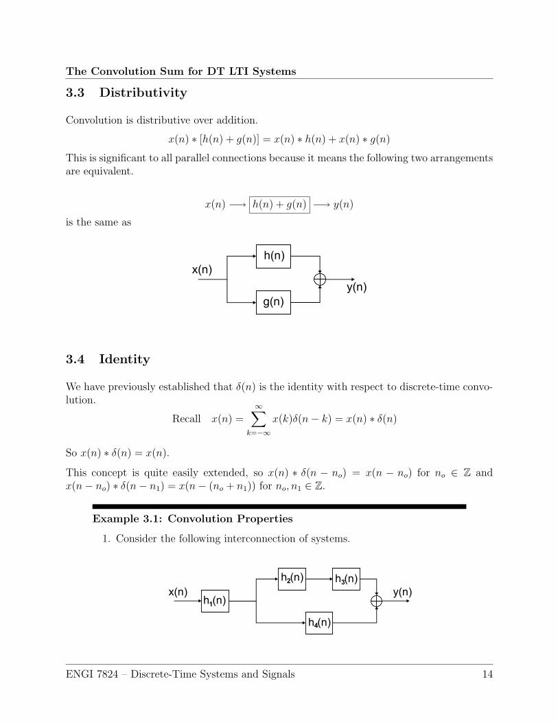
3.3 Distributivity

Convolution is distributive over addition.

x(n) ∗ [h(n) + g(n)] = x(n) ∗ h(n) + x(n) ∗ g(n)

This is significant to all parallel connections because it means the following two arrangementsare equivalent.

x(n) −→ h(n) + g(n) −→ y(n)

is the same as

3.4 Identity

We have previously established that δ(n) is the identity with respect to discrete-time convo-lution.

Recall x(n) =∞∑

k=−∞

x(k)δ(n− k) = x(n) ∗ δ(n)

So x(n) ∗ δ(n) = x(n).

This concept is quite easily extended, so x(n) ∗ δ(n − no) = x(n − no) for no ∈ Z andx(n− no) ∗ δ(n− n1) = x(n− (no + n1)) for no, n1 ∈ Z.

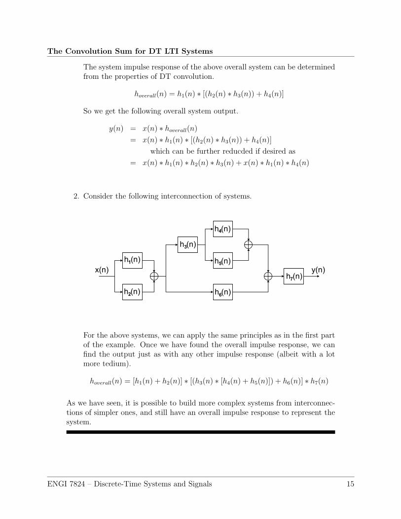
Example 3.1: Convolution Properties

1. Consider the following interconnection of systems.

ENGI 7824 – Discrete-Time Systems and Signals 14

The Convolution Sum for DT LTI Systems

The system impulse response of the above overall system can be determinedfrom the properties of DT convolution.

hoverall(n) = h1(n) ∗ [(h2(n) ∗ h3(n)) + h4(n)]

So we get the following overall system output.

y(n) = x(n) ∗ hoverall(n)

= x(n) ∗ h1(n) ∗ [(h2(n) ∗ h3(n)) + h4(n)]

which can be further reducded if desired as

= x(n) ∗ h1(n) ∗ h2(n) ∗ h3(n) + x(n) ∗ h1(n) ∗ h4(n)

2. Consider the following interconnection of systems.

For the above systems, we can apply the same principles as in the first partof the example. Once we have found the overall impulse response, we canfind the output just as with any other impulse response (albeit with a lotmore tedium).

hoverall(n) = [h1(n) + h2(n)] ∗ [(h3(n) ∗ [h4(n) + h5(n)]) + h6(n)] ∗ h7(n)

As we have seen, it is possible to build more complex systems from interconnec-tions of simpler ones, and still have an overall impulse response to represent thesystem.

ENGI 7824 – Discrete-Time Systems and Signals 15