Some DIC slides

David Spiegelhalter

MRC Biostatistics Unit, Cambridge

with thanks to:

Nicky BestDave Lunn

Andrew Thomas

IceBUGS: Finland, 11th-12th February 2006

c©MRC Biostatistics Unit 2006

1

Model comparison

What is the ‘deviance’?

• For a likelihood p(y|θ), we define the deviance as

D(θ) = −2 log p(y|θ) (1)

• In WinBUGS the quantity deviance is automatically calculated, where θ arethe parameters that appear in the stated sampling distribution of y

• The full normalising constants for p(y|θ) are included in deviance

• e.g. for Binomial data y[i] dbin(theta[i],n[i]), the deviance is

−2

∑

i

yi log θi + (ni − yi) log(1 − θi) + log

ni

ri

2

DIC slides 2006

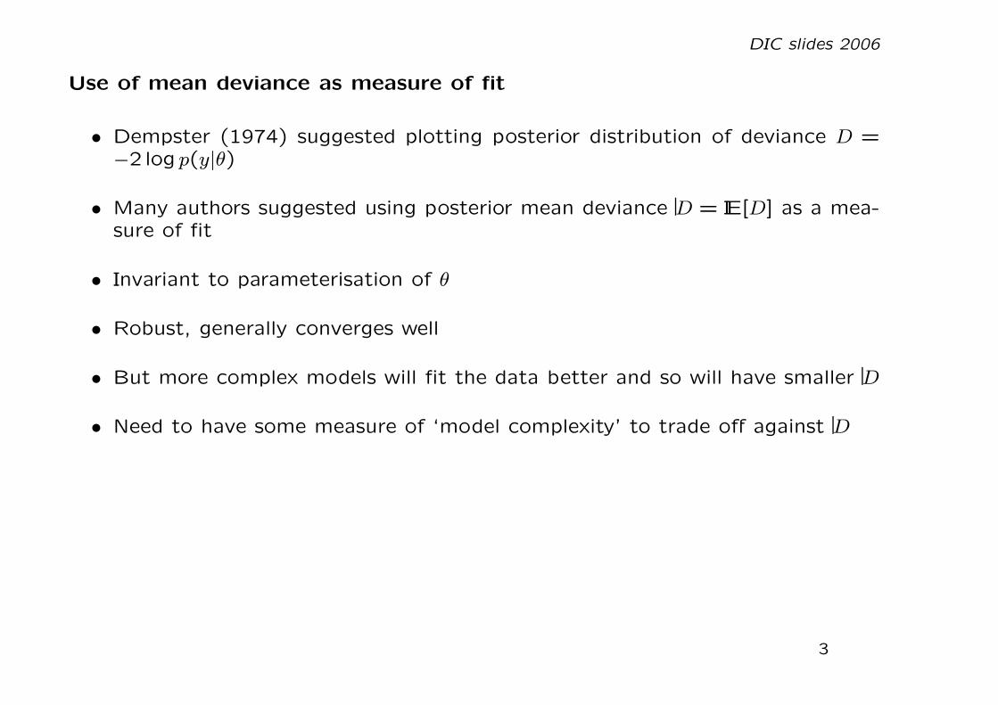
Use of mean deviance as measure of fit

• Dempster (1974) suggested plotting posterior distribution of deviance D =−2 log p(y|θ)

• Many authors suggested using posterior mean deviance D = IE[D] as a mea-sure of fit

• Invariant to parameterisation of θ

• Robust, generally converges well

• But more complex models will fit the data better and so will have smaller D

• Need to have some measure of ‘model complexity’ to trade off against D

3

DIC slides 2006

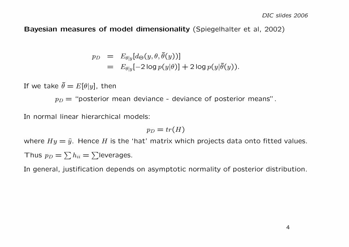
Bayesian measures of model dimensionality (Spiegelhalter et al, 2002)

pD = Eθ|y[dΘ(y, θ, θ(y))]

= Eθ|y[−2 log p(y|θ)] + 2 log p(y|θ(y)).

If we take θ = E[θ|y], then

pD = “posterior mean deviance - deviance of posterior means”.

In normal linear hierarchical models:

pD = tr(H)

where Hy = y. Hence H is the ‘hat’ matrix which projects data onto fitted values.

Thus pD =∑

hii =∑

leverages.

In general, justification depends on asymptotic normality of posterior distribution.

4

DIC slides 2006

Bayesian model comparison using DIC

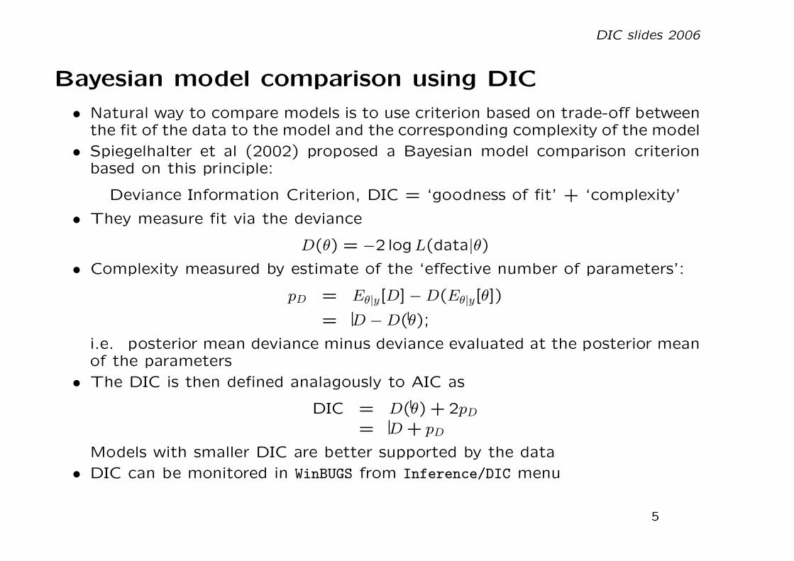
• Natural way to compare models is to use criterion based on trade-off betweenthe fit of the data to the model and the corresponding complexity of the model

• Spiegelhalter et al (2002) proposed a Bayesian model comparison criterionbased on this principle:

Deviance Information Criterion, DIC = ‘goodness of fit’ + ‘complexity’

• They measure fit via the deviance

D(θ) = −2 logL(data|θ)

• Complexity measured by estimate of the ‘effective number of parameters’:

pD = Eθ|y[D]−D(Eθ|y[θ])

= D −D(θ);

i.e. posterior mean deviance minus deviance evaluated at the posterior meanof the parameters

• The DIC is then defined analagously to AIC as

DIC = D(θ) + 2pD= D+ pD

Models with smaller DIC are better supported by the data

• DIC can be monitored in WinBUGS from Inference/DIC menu

5

DIC slides 2006

• These quantities are easy to compute in an MCMC run

• Aiming for Akaike-like, cross-validatory, behaviour based on ability to makeshort-term predictions of a repeat set of similar data.

• Not a function of the marginal likelihood of the data, so not aiming for Bayesfactor behaviour.

• Do not believe there is any ‘true’ model.

• pD is not invariant to reparameterisation (subject of much criticism).

• pD can be negative!

• Alternative to pD suggested

6

DIC slides 2006

pV : an alternative measure of complexity

• Suppose have non-hierarchical model with weak prior

• Then

D(θ) ≈ D(θ) + χ2I :

so that IE(D(θ)) ≈ D(θ) + I (leading to pD ≈ I as shown above), andVar(D(θ)) ≈ 2I.

• Thus with negligible prior information, half the variance of the deviance is anestimate of the number of free parameters in the model

• This estimate generally turns out to be remarkably robust and accurate

• Invariant to parameterisation

• This might suggest using pV = Var(D)/2 as an estimate of the effective num-ber of parameters in a model in more general situations: this was originallytried in a working paper by Spiegelhalter et al (1997), and has since beensuggested by Gelman et al (2004).

7

• Working through distribution theory for simple Normal random-effects modelwith I groups suggests

pV ≈ pD(2 − pD/I)

, but many assumptions

• So may expect pV to be larger than pD when there is moderate shrinkage.

DIC slides 2006

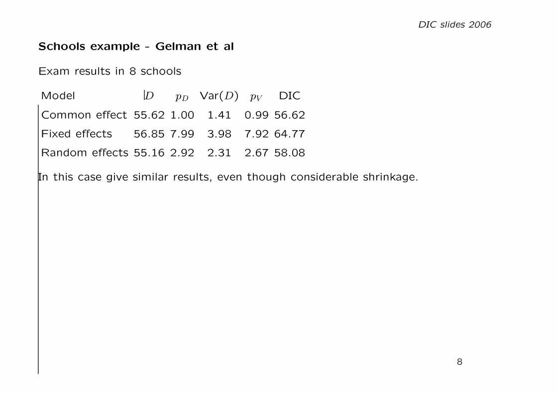
Schools example - Gelman et al

Exam results in 8 schools

Model D pD Var(D) pV DIC

Common effect 55.62 1.00 1.41 0.99 56.62

Fixed effects 56.85 7.99 3.98 7.92 64.77

Random effects 55.16 2.92 2.31 2.67 58.08

In this case give similar results, even though considerable shrinkage.

8

DIC slides 2006

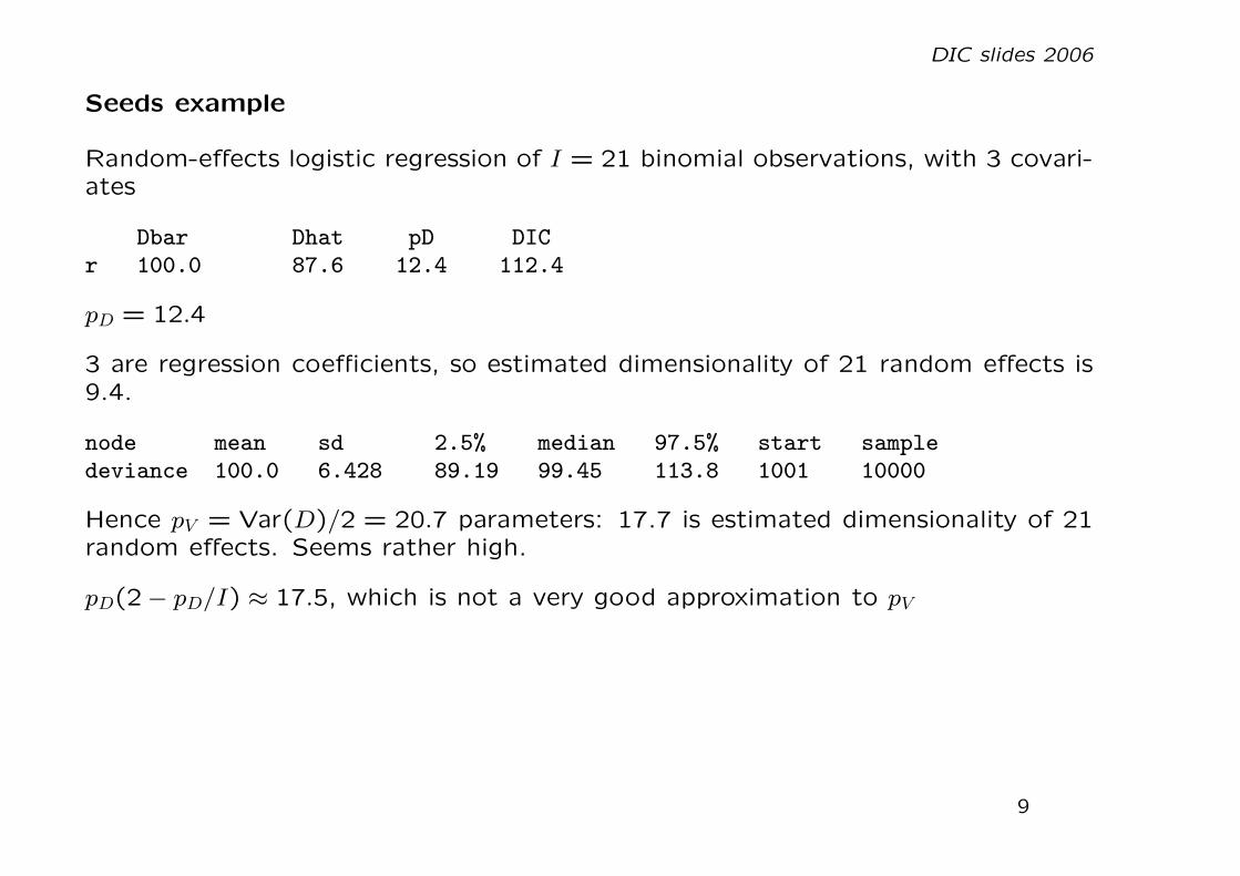
Seeds example

Random-effects logistic regression of I = 21 binomial observations, with 3 covari-ates

Dbar Dhat pD DICr 100.0 87.6 12.4 112.4

pD = 12.4

3 are regression coefficients, so estimated dimensionality of 21 random effects is9.4.

node mean sd 2.5% median 97.5% start sampledeviance 100.0 6.428 89.19 99.45 113.8 1001 10000

Hence pV = Var(D)/2 = 20.7 parameters: 17.7 is estimated dimensionality of 21random effects. Seems rather high.

pD(2 − pD/I) ≈ 17.5, which is not a very good approximation to pV

9

DIC slides 2006

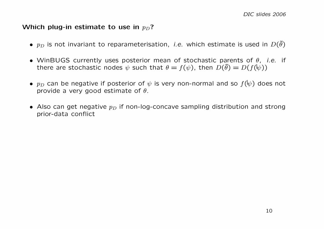
Which plug-in estimate to use in pD?

• pD is not invariant to reparameterisation, i.e. which estimate is used in D(θ)

• WinBUGS currently uses posterior mean of stochastic parents of θ, i.e. ifthere are stochastic nodes ψ such that θ = f(ψ), then D(θ) = D(f(ψ))

• pD can be negative if posterior of ψ is very non-normal and so f(ψ) does notprovide a very good estimate of θ.

• Also can get negative pD if non-log-concave sampling distribution and strongprior-data conflict

10

DIC slides 2006

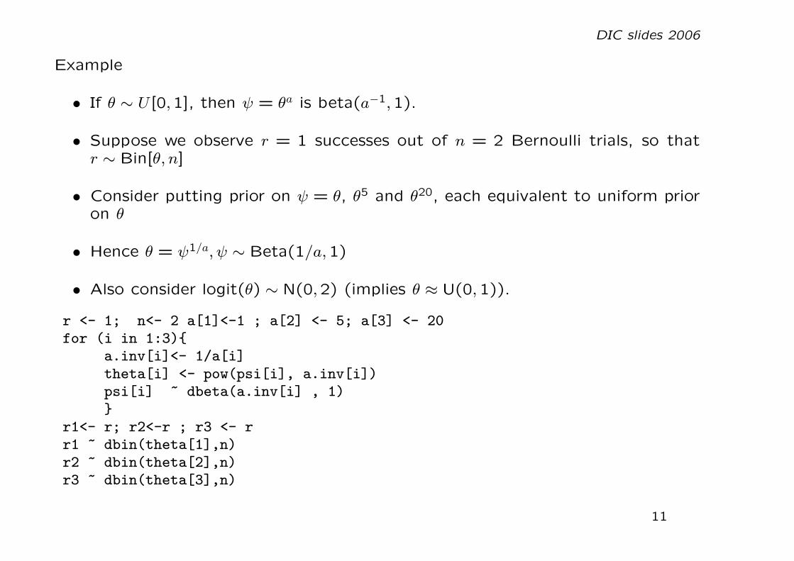
Example

• If θ ∼ U [0,1], then ψ = θa is beta(a−1,1).

• Suppose we observe r = 1 successes out of n = 2 Bernoulli trials, so thatr ∼ Bin[θ, n]

• Consider putting prior on ψ = θ, θ5 and θ20, each equivalent to uniform prioron θ

• Hence θ = ψ1/a, ψ ∼ Beta(1/a,1)

• Also consider logit(θ) ∼ N(0,2) (implies θ ≈ U(0,1)).

r <- 1; n<- 2 a[1]<-1 ; a[2] <- 5; a[3] <- 20for (i in 1:3){

a.inv[i]<- 1/a[i]theta[i] <- pow(psi[i], a.inv[i])psi[i] ~ dbeta(a.inv[i] , 1)}

r1<- r; r2<-r ; r3 <- rr1 ~ dbin(theta[1],n)r2 ~ dbin(theta[2],n)r3 ~ dbin(theta[3],n)

11

DIC slides 2006

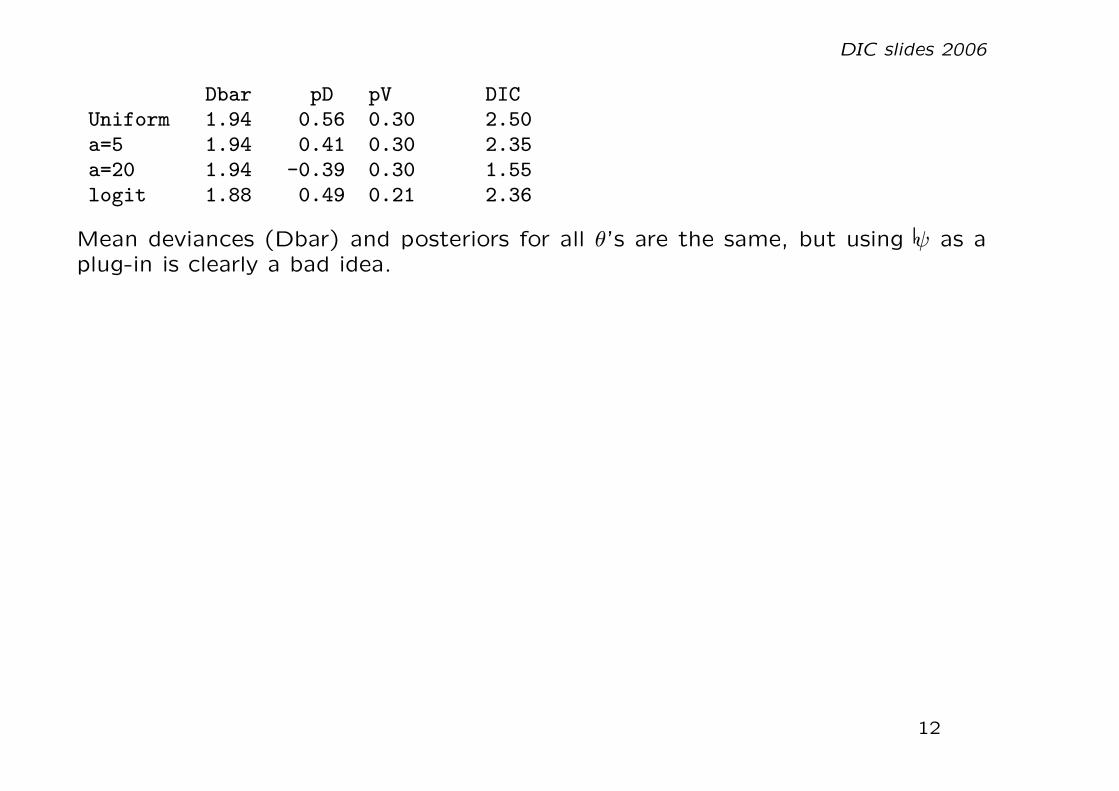
Dbar pD pV DICUniform 1.94 0.56 0.30 2.50a=5 1.94 0.41 0.30 2.35a=20 1.94 -0.39 0.30 1.55logit 1.88 0.49 0.21 2.36

Mean deviances (Dbar) and posteriors for all θ’s are the same, but using ψ as aplug-in is clearly a bad idea.

12

DIC slides 2006

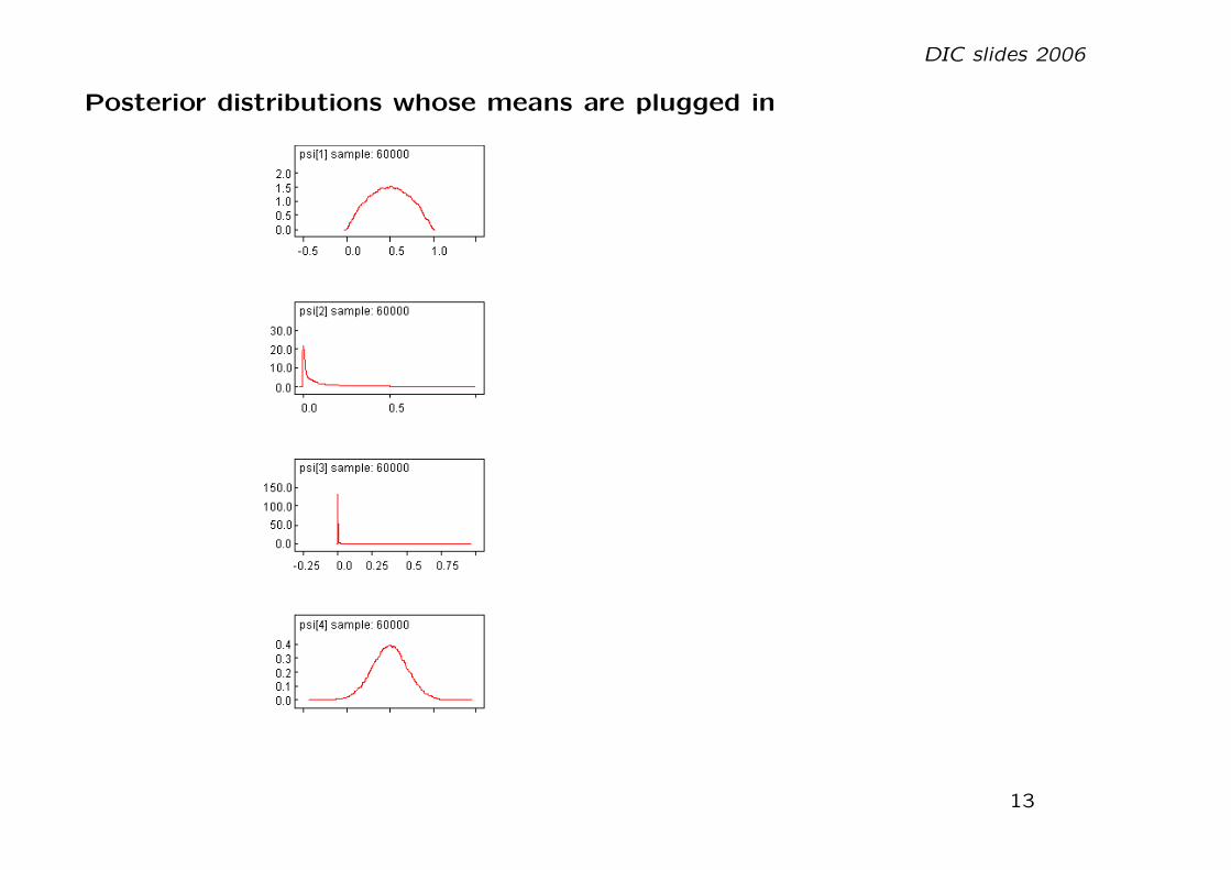
Posterior distributions whose means are plugged in

13

DIC slides 2006

What should we do about it?

• It would be better if WinBUGS used the posterior mean of the ‘direct param-eters’ (eg those that appear in the WinBUGS distribution syntax) to give a’plug-in’ deviance, rather than the posterior means of the stochastic parents.

• Users are free to calculate this themselves: could dump out posterior meansof ‘direct’ parameters in likelihood, then calculate deviance outside WinBUGSor by reading posterior means in as data and checking deviance in node info

• Lesson: need to be careful with highly non-linear models, where posteriormeans may not lead to good predictive estimates

• Same problem arises with mixture models

14

DIC slides 2006

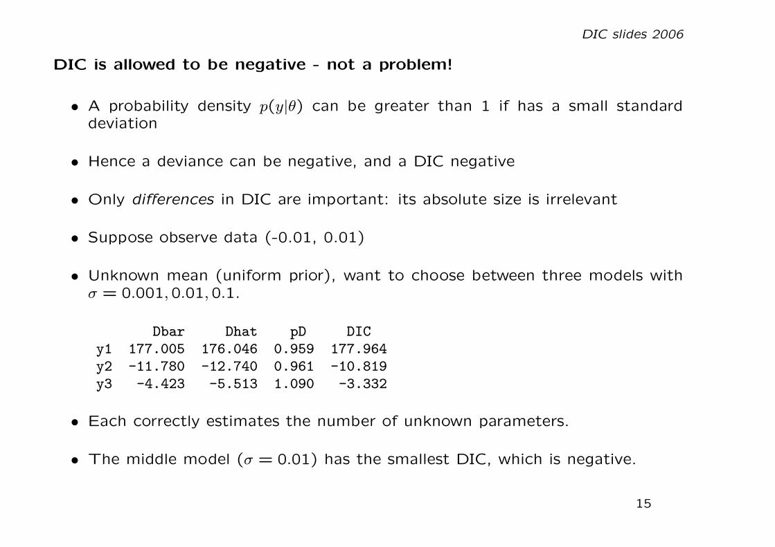
DIC is allowed to be negative - not a problem!

• A probability density p(y|θ) can be greater than 1 if has a small standarddeviation

• Hence a deviance can be negative, and a DIC negative

• Only differences in DIC are important: its absolute size is irrelevant

• Suppose observe data (-0.01, 0.01)

• Unknown mean (uniform prior), want to choose between three models withσ = 0.001,0.01,0.1.

Dbar Dhat pD DICy1 177.005 176.046 0.959 177.964y2 -11.780 -12.740 0.961 -10.819y3 -4.423 -5.513 1.090 -3.332

• Each correctly estimates the number of unknown parameters.

• The middle model (σ = 0.01) has the smallest DIC, which is negative.

15

DIC slides 2006

Why won’t DIC work with mixture likelihoods?

• WinBUGS currently ‘greys out’ DIC if the likelihood depends on any discreteparameters

• So cannot be used for mixture likelihoods

• Not clear what estimate to plug in for class membership indicator – mode?

• If mixture is represented marginally (ie not using an explicit indicator for classmembership), could use θ but could be taking mean of bimodal distributionand get poor estimate

• Celeux et al (2003) have made many suggestions

• Can still be used if prior (random effects) is a mixture

16

DIC slides 2006

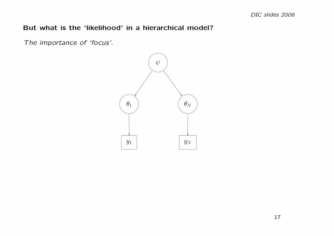
But what is the ‘likelihood’ in a hierarchical model?

The importance of ‘focus’.

onmlhijkψ

��

��66

6666

6666

6666

66

onmlhijkθ1

��

onmlhijkθN

��

y1 yN

17

DIC slides 2006

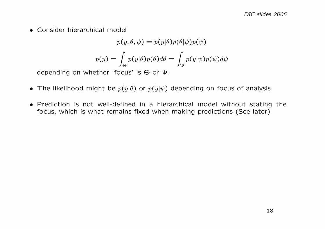
• Consider hierarchical model

p(y, θ, ψ) = p(y|θ)p(θ|ψ)p(ψ)

p(y) =

∫

Θ

p(y|θ)p(θ)dθ =

∫

Ψ

p(y|ψ)p(ψ)dψ

depending on whether ‘focus’ is Θ or Ψ.

• The likelihood might be p(y|θ) or p(y|ψ) depending on focus of analysis

• Prediction is not well-defined in a hierarchical model without stating thefocus, which is what remains fixed when making predictions (See later)

18

DIC slides 2006

What about alternatives for model comparison?

• DIC

DIC = D(θ) + 2pD

• AIC

AIC = −2 log p(y|ψ) + 2pψ

where pψ is the number of hyperparameters

• BIC

BIC = −2 log p(y|ψ) + pψ logn

An approximation to −2 log p(y), where

p(y) =

∫

Θ

p(y|θ)p(θ)dθ =

∫

Ψ

p(y|ψ)p(ψ)dψ

Depends on objective of analysis Vaida and Blanchard (2005) develop ‘conditional’AIC for when focus is random effects - this counts parameters using the ‘hat’matrix dimensionality p = tr(H), and so is restricted to normal linear models.

19

DIC slides 2006

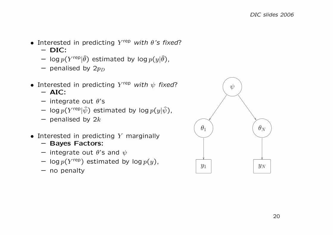
• Interested in predicting Y rep with θ’s fixed?– DIC:

– log p(Y rep|θ) estimated by log p(y|θ),

– penalised by 2pD

• Interested in predicting Y rep with ψ fixed?– AIC:

– integrate out θ’s

– log p(Y rep|ψ) estimated by log p(y|ψ),

– penalised by 2k

• Interested in predicting Y marginally– Bayes Factors:

– integrate out θ’s and ψ

– log p(Y rep) estimated by log p(y),

– no penalty

onmlhijkψ

��

��66

6666

6666

6666

66

onmlhijkθ1

��

onmlhijkθN

��

y1 yN

20

DIC slides 2006

An example

• Suppose the three levels of our model concerned classes within schools withina country

• Then if we were interested in predicting results of future classes in thoseactual schools, then Θ is the focus and deviance-based methods such as DICare appropriate;

• If we were interested in predicting results of future schools in that coun-try, then Ψ is the focus and marginal-likelihood methods such as AIC areappropriate;

• If we were interested in predicting results for a new country, then no param-eters are in focus and Bayes factors are appropriate to compare models.

• This suggests that Bayes factors may in many circumstances be inappropriatemeasures by which to compare models

21