
Second-Order PMD in Optical Components - Home |...
6
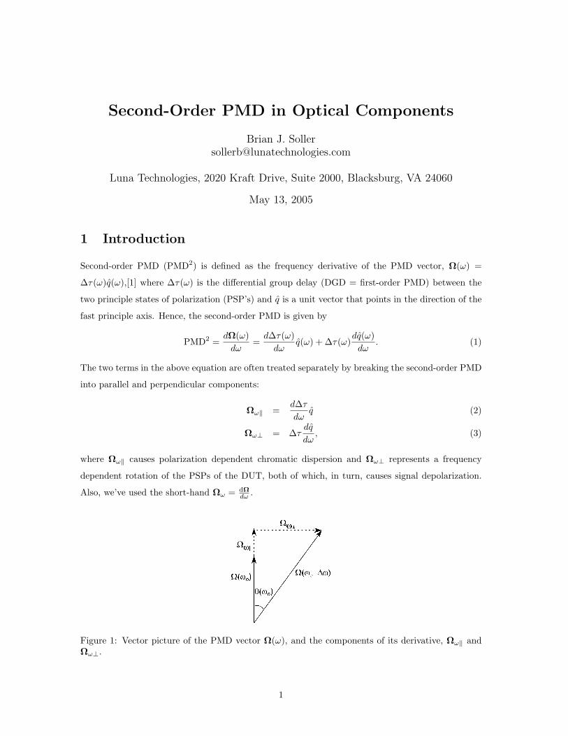
Second-Order PMD in Optical Components Brian J. Soller [email protected] Luna Technologies, 2020 Kraft Drive, Suite 2000, Blacksburg, VA 24060 May 13, 2005 1 Introduction Second-order PMD (PMD 2 ) is defined as the frequency derivative of the PMD vector, Ω(ω)= Δτ (ω)ˆ q(ω),[1] where Δτ (ω) is the differential group delay (DGD = first-order PMD) between the two principle states of polarization (PSP’s) and ˆ q is a unit vector that points in the direction of the fast principle axis. Hence, the second-order PMD is given by PMD 2 = dΩ(ω) dω = dΔτ (ω) dω ˆ q(ω)+Δτ (ω) d ˆ q(ω) dω . (1) The two terms in the above equation are often treated separately by breaking the second-order PMD into parallel and perpendicular components: Ω ω = dΔτ dω ˆ q (2) Ω ω⊥ = Δτ d ˆ q dω , (3) where Ω ω causes polarization dependent chromatic dispersion and Ω ω⊥ represents a frequency dependent rotation of the PSPs of the DUT, both of which, in turn, causes signal depolarization. Also, we’ve used the short-hand Ω ω = dΩ dω . Figure 1: Vector picture of the PMD vector Ω(ω), and the components of its derivative, Ω ω and Ω ω⊥ . 1
Transcript of Second-Order PMD in Optical Components - Home |...
Second-Order PMD in Optical Components
Brian J. [email protected]
Luna Technologies, 2020 Kraft Drive, Suite 2000, Blacksburg, VA 24060
May 13, 2005
1 Introduction
Second-order PMD (PMD2) is defined as the frequency derivative of the PMD vector, Ω(ω) =
∆τ(ω)q(ω),[1] where ∆τ(ω) is the differential group delay (DGD = first-order PMD) between the
two principle states of polarization (PSP’s) and q is a unit vector that points in the direction of the
fast principle axis. Hence, the second-order PMD is given by
PMD2 =dΩ(ω)
dω=
d∆τ(ω)dω
q(ω) + ∆τ(ω)dq(ω)dω
. (1)
The two terms in the above equation are often treated separately by breaking the second-order PMD
into parallel and perpendicular components:
Ωω‖ =d∆τ
dωq (2)
Ωω⊥ = ∆τdq
dω, (3)
where Ωω‖ causes polarization dependent chromatic dispersion and Ωω⊥ represents a frequency
dependent rotation of the PSPs of the DUT, both of which, in turn, causes signal depolarization.
Also, we’ve used the short-hand Ωω = dΩdω .
Figure 1: Vector picture of the PMD vector Ω(ω), and the components of its derivative, Ωω‖ andΩω⊥.
1
grosecloseb
Text Box
Luna Technologies, 3157 State Street, Blacksburg, VA 24060
www.LunaTechnologies.com 2
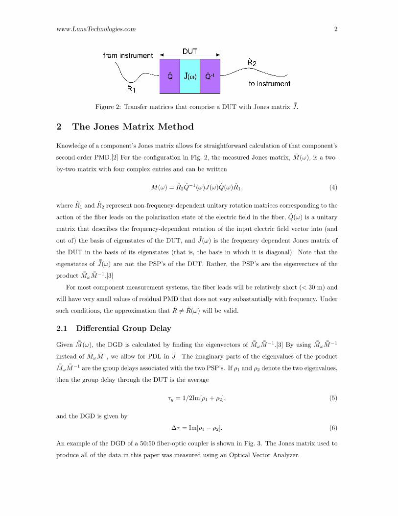
Figure 2: Transfer matrices that comprise a DUT with Jones matrix ¯J .
2 The Jones Matrix Method
Knowledge of a component’s Jones matrix allows for straightforward calculation of that component’s
second-order PMD.[2] For the configuration in Fig. 2, the measured Jones matrix, ¯M(ω), is a two-
by-two matrix with four complex entries and can be written
¯M(ω) = R2Q−1(ω) ¯J(ω)Q(ω)R1, (4)
where R1 and R2 represent non-frequency-dependent unitary rotation matrices corresponding to the
action of the fiber leads on the polarization state of the electric field in the fiber, Q(ω) is a unitary
matrix that describes the frequency-dependent rotation of the input electric field vector into (and
out of) the basis of eigenstates of the DUT, and ¯J(ω) is the frequency dependent Jones matrix of
the DUT in the basis of its eigenstates (that is, the basis in which it is diagonal). Note that the
eigenstates of ¯J(ω) are not the PSP’s of the DUT. Rather, the PSP’s are the eigenvectors of the
product ¯Mω¯M−1.[3]
For most component measurement systems, the fiber leads will be relatively short (< 30 m) and
will have very small values of residual PMD that does not vary subastantially with frequency. Under
such conditions, the approximation that R 6= R(ω) will be valid.
2.1 Differential Group Delay
Given ¯M(ω), the DGD is calculated by finding the eigenvectors of ¯Mω¯M−1.[3] By using ¯Mω
¯M−1
instead of ¯Mω¯M†, we allow for PDL in ¯J . The imaginary parts of the eigenvalues of the product
¯Mω¯M−1 are the group delays associated with the two PSP’s. If ρ1 and ρ2 denote the two eigenvalues,
then the group delay through the DUT is the average
τg = 1/2Im[ρ1 + ρ2], (5)
and the DGD is given by
∆τ = Im[ρ1 − ρ2]. (6)
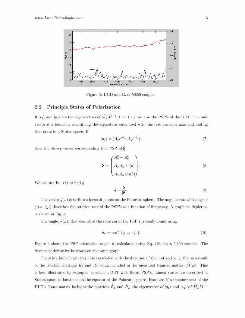
An example of the DGD of a 50:50 fiber-optic coupler is shown in Fig. 3. The Jones matrix used to
produce all of the data in this paper was measured using an Optical Vector Analyzer.
www.LunaTechnologies.com 3
Figure 3: DGD and IL of 50:50 coupler
2.2 Principle States of Polarization
If |s1〉 and |s2〉 are the eigenvectors of ¯Mω¯M−1, then they are also the PSP’s of the DUT. The unit
vector q is found by identifying the eigenstate associated with the fast principle axis and casting
that state in a Stokes space. If
|s1〉 = (Axeiδx , Ayeiδy ), (7)
then the Stokes vector corresponding that PSP is[4]
S =
A2
x − A2y
AxAy sin(δ)
AxAy cos(δ)
. (8)
We can use Eq. (8) to find q
q =S|S|
. (9)
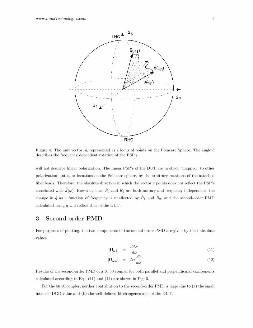
The vector q(ω) describes a locus of points on the Poincare sphere. The angular rate of change of
q (= |qω|) describes the rotation rate of the PSP’s as a function of frequency. A graphical depiction
is shown in Fig. 4
The angle, θ(ω), that describes the rotation of the PSP’s is easily found using
θn = cos−1(qn−1 · qn). (10)
Figure 4 shows the PSP orientation angle, θ, calculated using Eq. (10) for a 50:50 coupler. The
frequency derivative is shown on the same graph.
There is a built-in arbitrariness associated with the direction of the unit vector, q, that is a result
of the rotation matrices R1 and R2 being included in the measured transfer matrix, ¯M(ω). This
is best illustrated by example. consider a DUT with linear PSP’s. Linear states are described in
Stokes space as locations on the equator of the Poincare sphere. However, if a measurement of the
DUT’s Jones matrix includes the matrices R1 and R2, the eigenvector of |s1〉 and |s2〉 of ¯Mω¯M−1
www.LunaTechnologies.com 4
Figure 4: The unit vector, q, represented as a locus of points on the Poincare Sphere. The angle θdescribes the frequency dependent rotation of the PSP’s
will not describe linear polarization. The linear PSP’s of the DUT are in effect “mapped” to other
polarization states, or locations on the Poincare sphere, by the arbitrary rotations of the attached
fiber leads. Therefore, the absolute direction in which the vector q points does not reflect the PSP’s
associated with ¯J(ω). However, since R1 and R2 are both unitary and frequency independent, the
change in q as a function of frequency is unaffected by R1 and R2, and the second-order PMD
calculated using q will reflect that of the DUT.
3 Second-order PMD
For purposes of plotting, the two components of the second-order PMD are given by their absolute
values
|Ωω‖| =d∆τ
dω(11)
|Ωω⊥| = ∆τdθ
dω. (12)
Results of the second-order PMD of a 50:50 coupler for both parallel and perpendicular components
calculated according to Eqs. (11) and (12) are shown in Fig. 5.
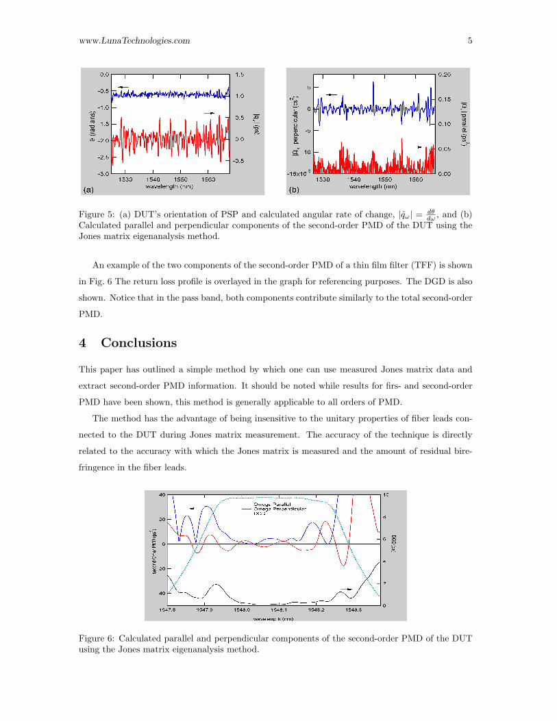
For the 50:50 coupler, neither contribution to the second-order PMD is large due to (a) the small
intrinsic DGD value and (b) the well defined birefringence axis of the DUT.
www.LunaTechnologies.com 5
Figure 5: (a) DUT’s orientation of PSP and calculated angular rate of change, |qω| = dθdω , and (b)
Calculated parallel and perpendicular components of the second-order PMD of the DUT using theJones matrix eigenanalysis method.
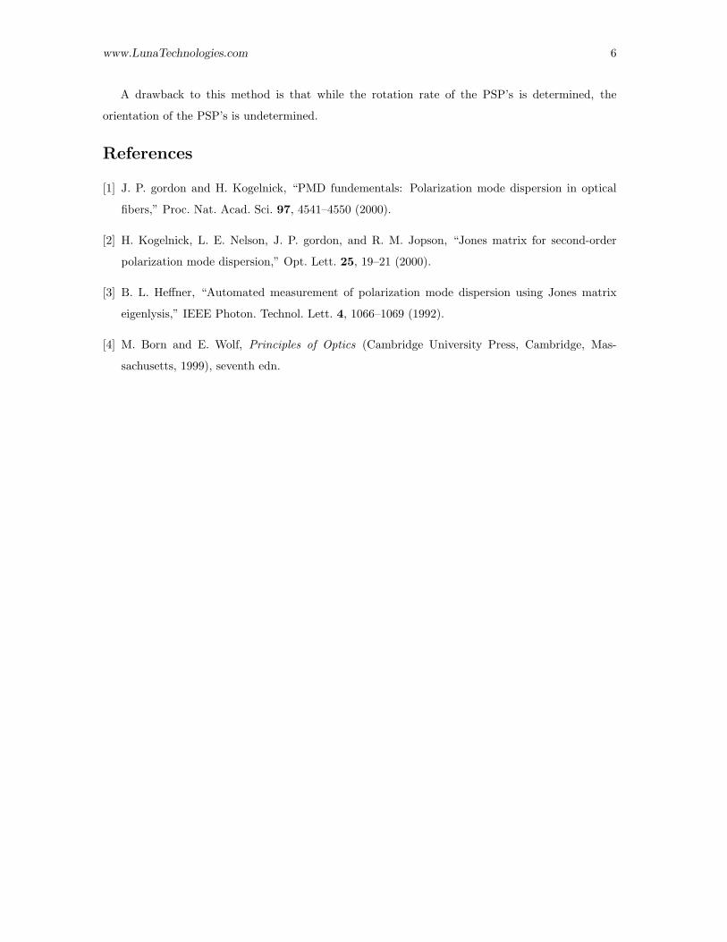
An example of the two components of the second-order PMD of a thin film filter (TFF) is shown
in Fig. 6 The return loss profile is overlayed in the graph for referencing purposes. The DGD is also
shown. Notice that in the pass band, both components contribute similarly to the total second-order
PMD.
4 Conclusions
This paper has outlined a simple method by which one can use measured Jones matrix data and
extract second-order PMD information. It should be noted while results for firs- and second-order
PMD have been shown, this method is generally applicable to all orders of PMD.
The method has the advantage of being insensitive to the unitary properties of fiber leads con-
nected to the DUT during Jones matrix measurement. The accuracy of the technique is directly
related to the accuracy with which the Jones matrix is measured and the amount of residual bire-
fringence in the fiber leads.
Figure 6: Calculated parallel and perpendicular components of the second-order PMD of the DUTusing the Jones matrix eigenanalysis method.
www.LunaTechnologies.com 6
A drawback to this method is that while the rotation rate of the PSP’s is determined, the
orientation of the PSP’s is undetermined.
References
[1] J. P. gordon and H. Kogelnick, “PMD fundementals: Polarization mode dispersion in optical
fibers,” Proc. Nat. Acad. Sci. 97, 4541–4550 (2000).
[2] H. Kogelnick, L. E. Nelson, J. P. gordon, and R. M. Jopson, “Jones matrix for second-order
polarization mode dispersion,” Opt. Lett. 25, 19–21 (2000).
[3] B. L. Heffner, “Automated measurement of polarization mode dispersion using Jones matrix
eigenlysis,” IEEE Photon. Technol. Lett. 4, 1066–1069 (1992).
[4] M. Born and E. Wolf, Principles of Optics (Cambridge University Press, Cambridge, Mas-
sachusetts, 1999), seventh edn.