On Buffon Machines and Numbers

Philippe Flajolet∗ Maryse Pelletier† Michele Soria†

philippe.flajolet@inria.fr, maryse.pelletier@lip6.fr, michele.soria@lip6.fr

AbstractThe well-know needle experiment of Buffon can be regardedas an analog (i.e., continuous) device that stochastically“computes” the number 2/π

.= 0.63661, which is the exper-

iment’s probability of success. Generalizing the experimentand simplifying the computational framework, we considerprobability distributions, which can be produced perfectly,from a discrete source of unbiased coin flips. We describeand analyse a few simple Buffon machines that generate ge-ometric, Poisson, and logarithmic-series distributions. Weprovide human-accessible Buffon machines, which require adozen coin flips or less, on average, and produce experimentswhose probabilities of success are expressible in terms ofnumbers such as π, exp(−1), log 2,

√3, cos( 1

4), ζ(5). Gener-

ally, we develop a collection of constructions based on sim-ple probabilistic mechanisms that enable one to design Buf-fon experiments involving compositions of exponentials andlogarithms, polylogarithms, direct and inverse trigonometricfunctions, algebraic and hypergeometric functions, as wellas functions defined by integrals, such as the Gaussian errorfunction.

Introduction

Buffon’s experiment (published in 1777) is as follows [1,4]. Take a plane marked with parallel lines at unitdistance from one another; throw a needle at random;finally, declare the experiment a success if the needleintersects one of the lines. Basic calculus implies thatthe probability of success is 2/π.

One can regard Buffon’s experiment as a simpleanalog device that takes as input real uniform [0, 1]–random variables (giving the position of the centreand the angle of the needle) and outputs a discrete{0, 1}–random variable, with 1 for success and 0 forfailure. The process then involves exact arithmeticoperations over real numbers. In the same vein, theclassical problem of simulating random variables canbe described as the construction of analog devices(algorithms) operating over the reals and equippedwith a real source of randomness, which are bothsimple and computationally efficient. The encyclopedictreatise of Devroye [6] provides many examples relative

∗Algorithms, INRIA, F-78153 Le Chesnay, France†LIP6, UPMC, 4, Place Jussieu, 75005 Paris, France

Law supp. distribution gen.

Bernoulli Ber(p) {0, 1} P(X = 1) = p ΓB(p)

geometric Geo(λ) Z≥0 P(X = r) = λr(1− λ) ΓG(λ)

Poisson, Poi(λ) Z≥0 P(X = r) = e−λ λr

r!ΓP(λ)

logarithmic, Log(λ) Z≥0 P(X = r) =1

L

λr

rΓL(λ)

Figure 1: Main discrete probability laws: support, expres-sion of the probabilities, and naming convention for genera-tors (L := log(1− λ)−1).

to the simulation of distributions, such as Gaussian,exponential, Cauchy, stable, and so on.

Buffon machines. Our objective is the perfectsimulation of discrete random variables (i.e., variablessupported by Z or one of its subsets; see Fig. 1). In thiscontext, it is natural to start with a discrete source ofrandomness that produces uniform random bits (ratherthan uniform [0, 1] real numbers), since we are interestedin finite computation (rather than infinite-precision realnumbers); cf Fig. 2.

Definition 1. A Buffon machine is a deterministic de-vice belonging to a computationally universal class (Tur-ing machines, equivalently, register machines), equippedwith an external source of independent uniform randombits and input–output queues capable of storing integers(usually, {0, 1}-bits), which is assumed to halt1 withprobability 1.

The fundamental question is then the following. Howdoes one generate, exactly and efficiently, discrete dis-tributions using only a discrete source of random bitsand finitary computations? A pioneering work in thisdirection is that of Knuth and Yao [20] who discussthe power of various restricted devices (e.g., finite-statemachines). Knuth’s treatment [18, §3.4] and the arti-cles [11, 36] provide additional results along these lines.

1Machines that always halt can only produce Bernoulli distri-

butions whose parameter is a dyadic rational s/2t; see [20] and §1.

In ACM-SIAM Symp. on Discrete Algorithms (SODA), 2011

--- 1 ----

inputs output

flips

Registers

H T T

Finitecontrol

Figure 2: A Buffon machine with two inputs, one output,and three registers.

Our original motivation for studying discrete Buf-fon machines came from Boltzmann samplers for combi-natorial structures, following the approach of Duchon,Flajolet, Louchard, and Schaeffer [7] and Flajolet, Fusy,and Pivoteau [9]. The current implementations relie onreal number computations, and they require generatingdistributions such as geometric, Poisson, or logarithmic,with various ranges of parameters—since the objects ul-timately produced are discrete, it is natural to try andproduce them by purely discrete means.

Numbers. Here is an intriguing range of relatedissues. Let M be an input-free Buffon machine thatoutputs a random variable X, whose value lies in {0, 1}.It can be seen from the definition that such a machineM, when called repeatedly, produces an independentsequence of Bernoulli random variables. We say thatM is a Buffon machine or Buffon computer for thenumber p := P(X = 1). We seek simple mechanisms—Buffon machines—that produce, from uniform {0, 1}-bits, Bernoulli variables whose probabilities of successare numbers such as

1/√

2, e−1, log 2,1π, π − 3,

1e− 1

.(0.1)

This problem can be seen as a vast generalization ofBuffon’s needle problem, adapted to the discrete world.

Complexity and simplicity. We will impose theloosely defined constraint that the Buffon machines weconsider be short and conceptually simple, to the extentof being easily implemented by a human. Thus, emulat-ing infinite-precision computation with multiprecisioninterval arithmetics or appealing to functions of highcomplexity as primitives is disallowed2. Our Buffon pro-grams only make use of simple integer counters, string

2The informal requirement of “simplicity” can be captured

by the formal notion of program size. All the programs we de-

registers (§2) and stacks (§3), as well as “bags” (§4).The reader may try her hand at determining Buffon-ness in this sense of some of the numbers listed in (0.1).We shall, for instance, produce a Buffon computer forthe constant Li3(1/2) of Eq. (2.11) (which involves log 2,π, and ζ(3)), one that is human-compatible, that con-sumes on average less than 6 coin flips, and that requiresat most 20 coin flips in 95% of the simulations. We shallalso devise nine different ways of simulating Bernoullidistributions whose probability involves π, some requir-ing as little as five coin flips on average. Furthermore,the constructions of this paper can all be encapsulatedinto a universal interpreter, briefly discussed in Sec-tion 5, which has less than 60 lines of Maple code andproduces all the constants of Eq. (0.1), as well as manymore.

In this extended abstract, we focus the discussionon algorithmic design. Analytic estimates can be ap-proached by means of (probability, counting) generatingfunctions in the style of methods of analytic combina-torics [12]; see the typical discussion in Subsection 2.1.The main results are Theorem 2.2 (Poisson and loga-rithmic generators), Theorem 2.3 (realizability of exps,logs, and trigs), Theorem 4.1 (general integrator), andTheorem 4.2 (inverse trig functions).

1 Framework and examples

Our approach consists in setting up a system basedon the composition of simple probabilistic experiments,corresponding to simple computing devices. (For thisreason, the Buffon machines of Definition 1 are allowedinput/output registers.) The unbiased random-bit gen-erator3, with which Buffon machines are equipped willbe named “flip”. The cost measure of a computation(simulation) is taken to be the number of flips. (For therestricted devices we shall consider, the overall simula-tion cost is essentially proportional to this measure.)

Definition 2. The function λ 7→ φ(λ), defined forλ ∈ (0, 1) and with values φ(λ) ∈ (0, 1), is said tobe weakly realizable if there is a machine M, which,

velop necessitate at most a few dozen register-machine instruc-

tions, see §5 and the Appendix, as opposed to programs basedon arbitrary-precision arithmetics, which must be rather huge;

cf [31]. If program size is unbounded, the problem becomes triv-

ial, since any Turing-computable number α can be emulated bya Buffon machine with a number of coin flips that is O(1) on av-

erage, e.g., by computing the sequence of digits of α on demand;

see [20] and Eq. (1.5) below.3This convention entails no loss of generality. Indeed, as first

observed by von Neumann, suppose we only have a biased coin,

where P(1) = p, P(0) = 1 − p, with p ∈ (0, 1). Then, one shouldtoss the coin twice: if 01 is observed, then output 0; if 10 is

observed, then output 1; otherwise, repeat with new coin tosses.

See, e.g., [20, 28] for more on this topic.

--- 2 ----

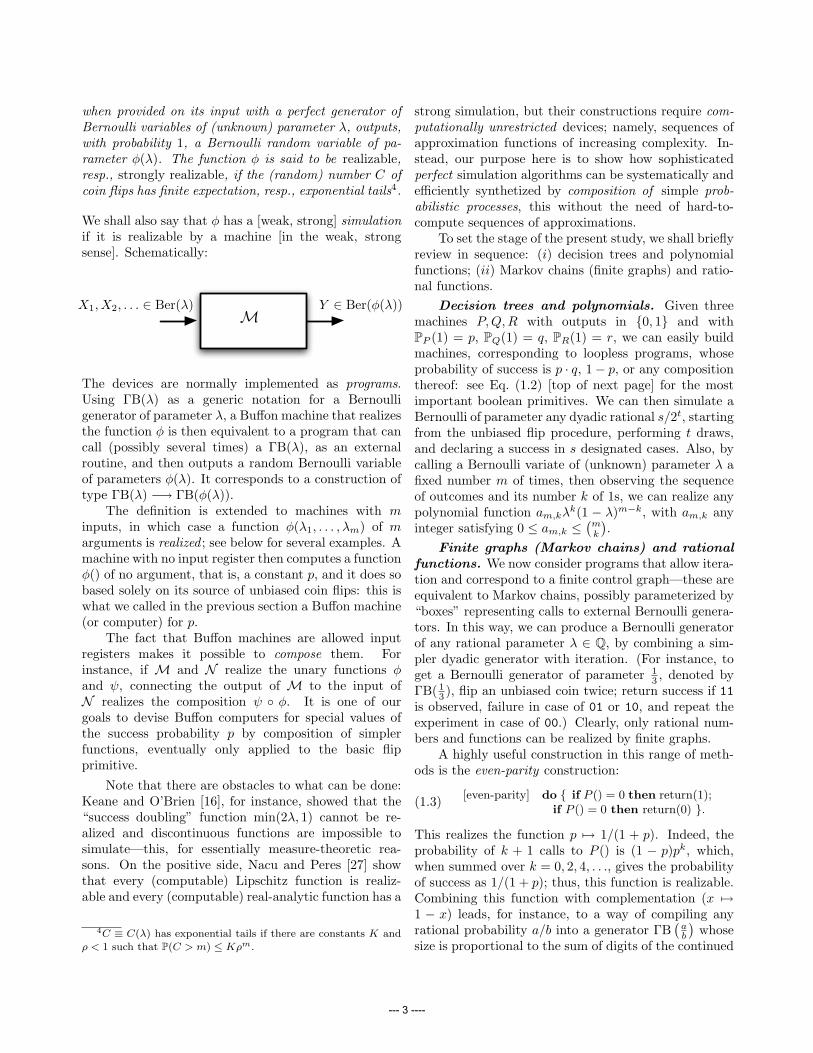
when provided on its input with a perfect generator ofBernoulli variables of (unknown) parameter λ, outputs,with probability 1, a Bernoulli random variable of pa-rameter φ(λ). The function φ is said to be realizable,resp., strongly realizable, if the (random) number C ofcoin flips has finite expectation, resp., exponential tails4.

We shall also say that φ has a [weak, strong] simulationif it is realizable by a machine [in the weak, strongsense]. Schematically:

X1, X2, . . . ∈ Ber(λ) Y ∈ Ber(φ(λ))M

The devices are normally implemented as programs.Using ΓB(λ) as a generic notation for a Bernoulligenerator of parameter λ, a Buffon machine that realizesthe function φ is then equivalent to a program that cancall (possibly several times) a ΓB(λ), as an externalroutine, and then outputs a random Bernoulli variableof parameters φ(λ). It corresponds to a construction oftype ΓB(λ) −→ ΓB(φ(λ)).

The definition is extended to machines with minputs, in which case a function φ(λ1, . . . , λm) of marguments is realized ; see below for several examples. Amachine with no input register then computes a functionφ() of no argument, that is, a constant p, and it does sobased solely on its source of unbiased coin flips: this iswhat we called in the previous section a Buffon machine(or computer) for p.

The fact that Buffon machines are allowed inputregisters makes it possible to compose them. Forinstance, if M and N realize the unary functions φand ψ, connecting the output of M to the input ofN realizes the composition ψ ◦ φ. It is one of ourgoals to devise Buffon computers for special values ofthe success probability p by composition of simplerfunctions, eventually only applied to the basic flipprimitive.

Note that there are obstacles to what can be done:Keane and O’Brien [16], for instance, showed that the“success doubling” function min(2λ, 1) cannot be re-alized and discontinuous functions are impossible tosimulate—this, for essentially measure-theoretic rea-sons. On the positive side, Nacu and Peres [27] showthat every (computable) Lipschitz function is realiz-able and every (computable) real-analytic function has a

4C ≡ C(λ) has exponential tails if there are constants K and

ρ < 1 such that P(C > m) ≤ Kρm.

strong simulation, but their constructions require com-putationally unrestricted devices; namely, sequences ofapproximation functions of increasing complexity. In-stead, our purpose here is to show how sophisticatedperfect simulation algorithms can be systematically andefficiently synthetized by composition of simple prob-abilistic processes, this without the need of hard-to-compute sequences of approximations.

To set the stage of the present study, we shall brieflyreview in sequence: (i) decision trees and polynomialfunctions; (ii) Markov chains (finite graphs) and ratio-nal functions.

Decision trees and polynomials. Given threemachines P,Q,R with outputs in {0, 1} and withPP (1) = p, PQ(1) = q, PR(1) = r, we can easily buildmachines, corresponding to loopless programs, whoseprobability of success is p · q, 1− p, or any compositionthereof: see Eq. (1.2) [top of next page] for the mostimportant boolean primitives. We can then simulate aBernoulli of parameter any dyadic rational s/2t, startingfrom the unbiased flip procedure, performing t draws,and declaring a success in s designated cases. Also, bycalling a Bernoulli variate of (unknown) parameter λ afixed number m of times, then observing the sequenceof outcomes and its number k of 1s, we can realize anypolynomial function am,kλ

k(1 − λ)m−k, with am,k anyinteger satisfying 0 ≤ am,k ≤

(mk

).

Finite graphs (Markov chains) and rationalfunctions. We now consider programs that allow itera-tion and correspond to a finite control graph—these areequivalent to Markov chains, possibly parameterized by“boxes” representing calls to external Bernoulli genera-tors. In this way, we can produce a Bernoulli generatorof any rational parameter λ ∈ Q, by combining a sim-pler dyadic generator with iteration. (For instance, toget a Bernoulli generator of parameter 1

3 , denoted byΓB( 1

3 ), flip an unbiased coin twice; return success if 11is observed, failure in case of 01 or 10, and repeat theexperiment in case of 00.) Clearly, only rational num-bers and functions can be realized by finite graphs.

A highly useful construction in this range of meth-ods is the even-parity construction:

[even-parity] do { if P () = 0 then return(1);if P () = 0 then return(0) }.(1.3)

This realizes the function p 7→ 1/(1 + p). Indeed, theprobability of k + 1 calls to P () is (1 − p)pk, which,when summed over k = 0, 2, 4, . . ., gives the probabilityof success as 1/(1 + p); thus, this function is realizable.Combining this function with complementation (x 7→1 − x) leads, for instance, to a way of compiling anyrational probability a/b into a generator ΓB

(ab

)whose

size is proportional to the sum of digits of the continued

--- 3 ----

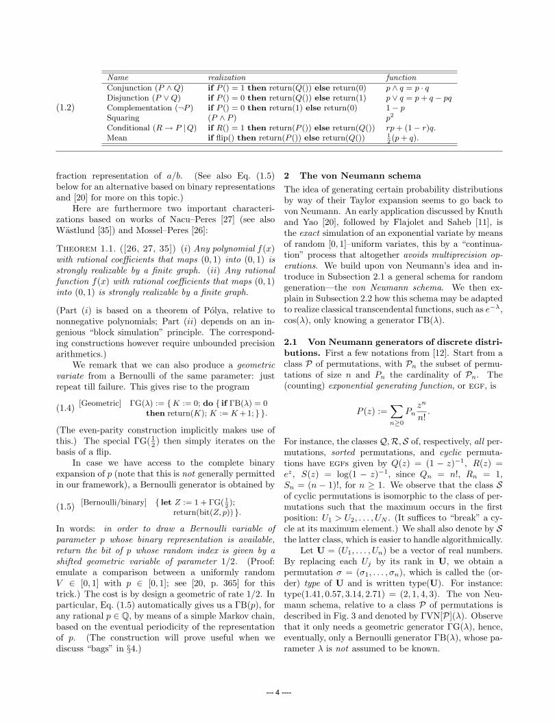
Name realization function

Conjunction (P ∧Q) if P () = 1 then return(Q()) else return(0) p ∧ q = p · qDisjunction (P ∨Q) if P () = 0 then return(Q()) else return(1) p ∨ q = p + q − pqComplementation (¬P ) if P () = 0 then return(1) else return(0) 1− pSquaring (P ∧ P ) p2

Conditional (R → P |Q) if R() = 1 then return(P ()) else return(Q()) rp + (1− r)q.Mean if flip() then return(P ()) else return(Q()) 1

2(p + q).

(1.2)

fraction representation of a/b. (See also Eq. (1.5)below for an alternative based on binary representationsand [20] for more on this topic.)

Here are furthermore two important characteri-zations based on works of Nacu–Peres [27] (see alsoWastlund [35]) and Mossel–Peres [26]:

Theorem 1.1. ([26, 27, 35]) (i) Any polynomial f(x)with rational coefficients that maps (0, 1) into (0, 1) isstrongly realizable by a finite graph. (ii) Any rationalfunction f(x) with rational coefficients that maps (0, 1)into (0, 1) is strongly realizable by a finite graph.

(Part (i) is based on a theorem of Polya, relative tononnegative polynomials; Part (ii) depends on an in-genious “block simulation” principle. The correspond-ing constructions however require unbounded precisionarithmetics.)

We remark that we can also produce a geometricvariate from a Bernoulli of the same parameter: justrepeat till failure. This gives rise to the program

[Geometric] ΓG(λ) := {K := 0; do { if ΓB(λ) = 0then return(K); K := K +1; } }.(1.4)

(The even-parity construction implicitly makes use ofthis.) The special ΓG(1

2 ) then simply iterates on thebasis of a flip.

In case we have access to the complete binaryexpansion of p (note that this is not generally permittedin our framework), a Bernoulli generator is obtained by

[Bernoulli/binary] { let Z := 1 + ΓG( 12);

return(bit(Z, p)) }.(1.5)

In words: in order to draw a Bernoulli variable ofparameter p whose binary representation is available,return the bit of p whose random index is given by ashifted geometric variable of parameter 1/2. (Proof:emulate a comparison between a uniformly randomV ∈ [0, 1] with p ∈ [0, 1]; see [20, p. 365] for thistrick.) The cost is by design a geometric of rate 1/2. Inparticular, Eq. (1.5) automatically gives us a ΓB(p), forany rational p ∈ Q, by means of a simple Markov chain,based on the eventual periodicity of the representationof p. (The construction will prove useful when wediscuss “bags” in §4.)

2 The von Neumann schema

The idea of generating certain probability distributionsby way of their Taylor expansion seems to go back tovon Neumann. An early application discussed by Knuthand Yao [20], followed by Flajolet and Saheb [11], isthe exact simulation of an exponential variate by meansof random [0, 1]–uniform variates, this by a “continua-tion” process that altogether avoids multiprecision op-erations. We build upon von Neumann’s idea and in-troduce in Subsection 2.1 a general schema for randomgeneration—the von Neumann schema. We then ex-plain in Subsection 2.2 how this schema may be adaptedto realize classical transcendental functions, such as e−λ,cos(λ), only knowing a generator ΓB(λ).

2.1 Von Neumann generators of discrete distri-butions. First a few notations from [12]. Start from aclass P of permutations, with Pn the subset of permu-tations of size n and Pn the cardinality of Pn. The(counting) exponential generating function, or egf, is

P (z) :=∑n≥0

Pnzn

n!.

For instance, the classesQ,R,S of, respectively, all per-mutations, sorted permutations, and cyclic permuta-tions have egfs given by Q(z) = (1 − z)−1, R(z) =ez, S(z) = log(1 − z)−1, since Qn = n!, Rn = 1,Sn = (n − 1)!, for n ≥ 1. We observe that the class Sof cyclic permutations is isomorphic to the class of per-mutations such that the maximum occurs in the firstposition: U1 > U2, . . . , UN . (It suffices to “break” a cy-cle at its maximum element.) We shall also denote by Sthe latter class, which is easier to handle algorithmically.

Let U = (U1, . . . , Un) be a vector of real numbers.By replacing each Uj by its rank in U, we obtain apermutation σ = (σ1, . . . , σn), which is called the (or-der) type of U and is written type(U). For instance:type(1.41, 0.57, 3.14, 2.71) = (2, 1, 4, 3). The von Neu-mann schema, relative to a class P of permutations isdescribed in Fig. 3 and denoted by ΓVN[P](λ). Observethat it only needs a geometric generator ΓG(λ), hence,eventually, only a Bernoulli generator ΓB(λ), whose pa-rameter λ is not assumed to be known.

--- 4 ----

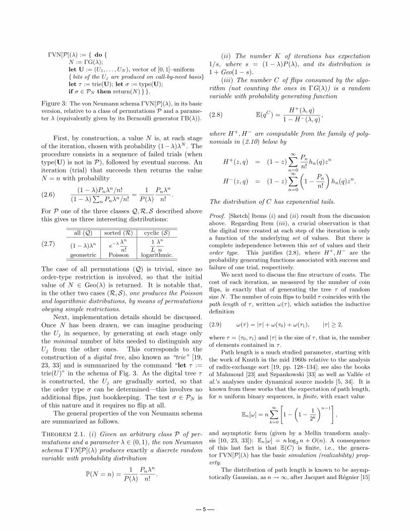
ΓVN[P](λ) := { do {N := ΓG(λ);let U := (U1, . . . , UN ), vector of [0, 1]–uniform{ bits of the Uj are produced on call-by-need basis}let τ := trie(U); let σ := type(U);if σ ∈ PN then return(N) } }.

Figure 3: The von Neumann schema ΓVN[P](λ), in its basicversion, relative to a class of permutations P and a parame-ter λ (equivalently given by its Bernoulli generator ΓB(λ)).

First, by construction, a value N is, at each stageof the iteration, chosen with probability (1−λ)λN . Theprocedure consists in a sequence of failed trials (whentype(U) is not in P), followed by eventual success. Aniteration (trial) that succeeds then returns the valueN = n with probability

(1− λ)Pnλn/n!

(1− λ)∑

n Pnλn/n!=

1P (λ)

Pnλn

n!.(2.6)

For P one of the three classes Q,R,S described abovethis gives us three interesting distributions:

all (Q) sorted (R) cyclic (S)

(1− λ)λn e−λ λn

n!

1

L

λn

ngeometric Poisson logarithmic.

(2.7)

The case of all permutations (Q) is trivial, since noorder-type restriction is involved, so that the initialvalue of N ∈ Geo(λ) is returned. It is notable that,in the other two cases (R,S), one produces the Poissonand logarithmic distributions, by means of permutationsobeying simple restrictions.

Next, implementation details should be discussed.Once N has been drawn, we can imagine producingthe Uj in sequence, by generating at each stage onlythe minimal number of bits needed to distinguish anyUj from the other ones. This corresponds to theconstruction of a digital tree, also known as “trie” [19,23, 33] and is summarized by the command “let τ :=trie(U)” in the schema of Fig. 3. As the digital tree τis constructed, the Uj are gradually sorted, so thatthe order type σ can be determined—this involves noadditional flips, just bookkeeping. The test σ ∈ PN isof this nature and it requires no flip at all.

The general properties of the von Neumann schemaare summarized as follows.

Theorem 2.1. (i) Given an arbitrary class P of per-mutations and a parameter λ ∈ (0, 1), the von Neumannschema ΓVN[P](λ) produces exactly a discrete randomvariable with probability distribution

P(N = n) =1

P (λ)Pnλ

n

n!.

(ii) The number K of iterations has expectation1/s, where s = (1− λ)P (λ), and its distribution is1 + Geo(1− s).

(iii) The number C of flips consumed by the algo-rithm (not counting the ones in ΓG(λ)) is a randomvariable with probability generating function

E(qC) =H+(λ, q)

1−H−(λ, q),(2.8)

where H+,H− are computable from the family of poly-nomials in (2.10) below by

H+(z, q) = (1− z)∞∑

n=0

Pn

n!hn(q)zn

H−(z, q) = (1− z)∞∑

n=0

(1− Pn

n!

)hn(q)zn.

The distribution of C has exponential tails.

Proof. [Sketch] Items (i) and (ii) result from the discussionabove. Regarding Item (iii), a crucial observation is thatthe digital tree created at each step of the iteration is onlya function of the underlying set of values. But there iscomplete independence between this set of values and theirorder type. This justifies (2.8), where H+, H− are theprobability generating functions associated with success andfailure of one trial, respectively.

We next need to discuss the fine structure of costs. Thecost of each iteration, as measured by the number of coinflips, is exactly that of generating the tree τ of randomsize N . The number of coin flips to build τ coincides with thepath length of τ , written ω(τ), which satisfies the inductivedefinition

ω(τ) = |τ |+ ω(τ0) + ω(τ1), |τ | ≥ 2,(2.9)

where τ = 〈τ0, τ1〉 and |τ | is the size of τ , that is, the numberof elements contained in τ .

Path length is a much studied parameter, starting withthe work of Knuth in the mid 1960s relative to the analysisof radix-exchange sort [19, pp. 128–134]; see also the booksof Mahmoud [23] and Szpankowski [33] as well as Vallee etal.’s analyses under dynamical source models [5, 34]. It isknown from these works that the expectation of path length,for n uniform binary sequences, is finite, with exact value

En[ω] = n

∞Xk=0

"1−

„1− 1

2k

«n−1#

,

and asymptotic form (given by a Mellin transform analy-sis [10, 23, 33]): En[ω] = n log2 n + O(n). A consequenceof this last fact is that E(C) is finite, i.e., the genera-tor ΓVN[P](λ) has the basic simulation (realizability) prop-erty.

The distribution of path length is known to be asymp-totically Gaussian, as n →∞, after Jacquet and Regnier [15]

--- 5 ----

and Mahmoud et al. [25]; see also [24, §11.2]. For our pur-poses, it suffices to note that the bivariate egf

H(z, q) :=

∞Xn=0

En[qω]zn

n!

satisfies the nonlinear functional equation H(z, q) =

H`

zq2

, q´2

+ z(1− q), with H(0, q) = 1. This equation fullydetermines H, since it is equivalent to a recurrence on coef-ficients, hn(q) := n![zn]H(z, q), for n ≥ 2:

hn(q) =1

1− qn21−n

n−1Xk=1

1

2n

n

k

!hk(q)hn−k(q).(2.10)

The computability of H+, H− then results. In addition,large deviation estimates can be deduced from (2.10), whichserve to establish exponential tails for C, thereby ensuringa strong simulation property in the sense of Definition 2.

A notable consequence of Theorem 2.1 is the possi-bility of generating a Poisson or logarithmic variate bya simple device: as we saw in the discussion precedingthe statement of the Theorem, only one branch of thetrie needs to be maintained, in the case of the classes Rand S of (2.7).

Theorem 2.2. The Poisson and logarithmic distribu-tions of parameter λ ∈ (0, 1) have a strong simulationby a Buffon machine, ΓVN[R](λ) and ΓVN[S](λ), re-spectively, which only uses a single string register.

Since the sum of two Poisson variates is Poisson(with rate the sum of the rates), the strong simulationresult extends to any X ∈ Poi(λ), for any λ ∈ R≥0.This answers an open question of Knuth and Yao in [20,p. 426]. We may also stress here that the distributionsof costs are easily computable: with the symbolicmanipulation system Maple, the cost of generatinga Poisson(1/2) variate is found to have probabilitygenerating function (Item (iii) of Theorem 2.1)

34

+7

128q2+

1194096

q4+19

1024q5+

2023131072

q6+179

16384q7+· · · .

Interestingly enough, the analysis of the logarithmicgenerators involves ideas similar to those relative to aclassical leader election protocol [8, 30].

2.2 Buffon computers: logarithms, exponen-tials, and trig functions. We can also take any ofthe previous constructions and specialize it by declar-ing a success whenever a special value N = a is re-turned, for some predetermined a (usually a = 0, 1),declaring a failure, otherwise. For instance, the Poissongenerator with a = 0 gives us in this way a Bernoulligenerator with parameter λ′ = exp(−λ). Since the

von Neumann machine only requires a Bernoulli gen-erator ΓB(λ), we thus have a purely discrete construc-tion ΓB(λ) −→ ΓB

(e−λ

). Similarly, the logarithmic

generator restricted to a = 1 provides a constructionΓB(λ) −→ ΓB

(λ

log(1−λ)−1

). Naturally, these construc-

tions can be enriched by the basic ones of Section 1, inparticular, complementation.

Another possibility is to make use of the numberK of iterations, which is a shifted geometric of rates = (1 − λ)P (λ); see Theorem 2.1, Item (ii). If wedeclare a success whenK = b, for some predetermined b,we then obtain yet another brand of generators. ThePoisson generator used in this way with b = 1 gives usΓB(λ) −→ ΓB

((1− λ)eλ

), ΓB

(λe1−λ

), where the

latter involves an additional complementation.Trigonometric functions can also be brought into

the game. A sequence U = (U1, . . . , Un) is said tobe alternating if U1 < U2 > U3 < U4 > · · ·. It iswell known that the egfs of the classes A+ of even-sized and A− of odd-sized permutations are respectivelyA+(z) = sec(z) = 1/cos(z), and A−(z) = tan(z) =sin(z)/cos(z). (This result, due to Desire Andre around1880, is in most books on combinatorial enumeration,e.g., [12, 13, 32].) Note that the property of beingalternating can once more be tested sequentially: onlya partial expansion of the current value of Uj needs tobe stored at any given instant. By making use of theproperties A+,A−, with, respectively N = 0, 1, we thenobtain new trigonometric constructions.

In summary:

Theorem 2.3. The following functions admit a strongsimulation:

e−x, ex−1, (1− x)ex, xe1−x,x

log(1− x)−1,

1− x

log(1/x), (1− x) log

11− x

, x log1x,

cos(x),1− x

cos(x),

x

tan(x), (1− x) tan(x).

2.3 Polylogarithmic constants. The probabilitythat a vector U is such that U1 > U2, . . . , Un (the firstelement is largest) equals 1/n, a property that underliesthe logarithmic series generator. By sequentially draw-ing r several such vectors and requiring success on all rtrials, we deduce constructions for families involving thepolylogarithmic functions, Lir(z) :=

∑∞n≥1 z

n/nr, withr ∈ Z≥1. Of course, Li1(1/2) = log 2. The few spe-cial evaluations known for polylogarithmic values (seethe books by Berndt on Ramanujan [3, Ch. 9] and byLewin [21, 22]) include Li2(1/2) = π2

12 −12 log2 2 and

Li3(1

2) =

log3 2

6− π2 log 2

12+

7ζ(3)

8, ζ(s) :=

Xn≥1

1

ns.(2.11)

--- 6 ----

By rational convex combinations, we obtain Buffoncomputers for π2

24 and 732ζ(3). Similarly, the celebrated

BBP (Bailey–Borwein–Plouffe) formulae [2] can be im-plemented as Buffon machines.

3 Square roots, algebraic, and hypergeometricfunctions

We now examine a new brand of generators based onproperties of ballot sequences, which open the way tonew constructions, including an important square-rootmechanism. The probability that, in 2n tosses of a faircoin, there are as many heads as tails is $n = 1

22n

(2nn

).

The property is easily testable with a single integercounter R subject only to the basic operation R := R±1and to the basic test R ?= 0. From this, one can build asquare-root computer and, by repeating the test, certainhypergeometric constants can be obtained.

3.1 Square-roots Let N be a random variable withdistribution Geo(λ). Assume we flip 2N coins andreturn a success, if the score of heads and tails isbalanced. The probability of success is

S(λ) :=∞∑

n=0

(1− λ)λn$n =√

1− λ.

(The final simplification is due to the binomial expan-sion of (1− x)−1/2.) This simple property gives rise tothe square-root construction due to Wastlund [35] andMossel–Peres [26]:

ΓB`√

1− λ´

:={ let N := ΓG(λ);draw X1, . . . , X2N with P(Xj = +1) = P(Xj = −1) = 1

2;

set ∆ :=P2N

j=0 Xj ;

if ∆ = 0 then return(1) else return(0) }.

The mean number of coin flips used is then simplyobtained by differentiation of generating functions.

Theorem 3.1. ([26, 35]) The square-root construc-tion yields a Bernoulli generator of parameter

√1− λ,

given a ΓB(λ). The mean number of coin flips required,not counting the ones involved in the calls to ΓB(λ), is2λ

1−λ . The function√

1− λ is strongly realizable.

By complementation of the original Bernoulli generator,we also have a construction ΓB(λ) −→ ΓB(1−λ) −→ΓB

(√λ), albeit one that is irregular at 0.

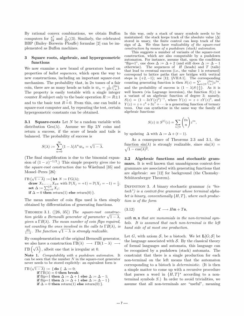
Note 1. Computability with a pushdown automaton. Itcan be seen that the number N in the square-root generatornever needs to be stored explicitly: an equivalent form is

ΓB`√

1− λ´

:= {do { ∆ := 0;if ΓB(λ) = 0 then break;if flip=1 then ∆ := ∆ + 1 else ∆ := ∆− 1;if flip=1 then ∆ := ∆ + 1 else ∆ := ∆− 1 }if ∆ = 0 then return(1) else return(0) }.

In this way, only a stack of unary symbols needs to bemaintained: the stack keeps track of the absolute value |∆|stored in unary, the finite control can keep track of thesign of ∆. We thus have realizability of the square-rootconstruction by means of a pushdown (stack) automaton.

This suggests a number of variants of the square-rootconstruction, which are also computable by a pushdownautomaton. For instance, assume that, upon the condition“flip=1”, one does ∆ := ∆ + 2 (and still does ∆ := ∆ − 1otherwise). The sequences of H (heads) and T (tails)that lead to eventual success (i.e., the value 1 is returned)correspond to lattice paths that are bridges with verticalsteps in {+2,−1}; see [12, §VII.8.1]. The correspondingcounting generating function is then S(z) =

Pn≥0

`3nn

´z3n,

and the probability of success is (1 − λ)S`

λ2

´. As it is

well known (via Lagrange inversion), the function S(z) isa variant of an algebraic function of degree 3; namely,S(z) = (1 − 3zY (z)2)−1, where Y (z) = z + zY (z)3, andY (z) = z + z4 + 3z7 + · · · is a generating function of ternarytrees. One can synthetize in the same way the family ofalgebraic functions

S(z) ≡ S[t](z) =Xn≥0

tn

n

!ztn,

by updating ∆ with ∆ := ∆ + (t− 1).

As a consequence of Theorems 2.3 and 3.1, thefunction sin(λ) is strongly realizable, since sin(λ) =√

1− cos(λ)2.

3.2 Algebraic functions and stochastic gram-mars. It is well known that unambiguous context-freegrammars are associated with generating functions thatare algebraic: see [12] for background (the Chomsky–Schutzenberger Theorem).

Definition 3. A binary stochastic grammar (a “bis-toch”) is a context-free grammar whose terminal alpha-bet is binary, conventionally {H,T}, where each produc-tion is of the form

X −→ Hm + Tn,(3.12)

with m, n that are monomials in the non-terminal sym-bols. It is assumed that each non-terminal is the lefthand side of at most one production.

Let G, with axiom S, be a bistoch. We let L[G;S] bethe language associated with S. By the classical theoryof formal languages and automata, this language canbe recognized by a pushdown (stack) automata. Theconstraint that there is a single production for eachnon-terminal on the left means that the automatoncorresponding to a bistoch is deterministic. (It is thena simple matter to come up with a recursive procedurethat parses a word in {H,T}? according to a non-terminal symbols S.) In order to avoid trivialities, weassume that all non-terminals are “useful”, meaning

--- 7 ----

{ let N := ΓG(λ);draw w := X1X2 · · ·XN with P(Xj = H) = P(Xj = T ) = 1

2;

if w ∈ L(G;S) then return(1) else return(0) }.

Figure 4: The algebraic construction associated to thepushdown automaton arising from a bistoch grammar.

that each produces at least one word of {H,T}?. Forinstance, the one-terminal grammar Y = HYYY + Tgenerates all Lukasiewicz codes of ternary trees [12,§I.5.3] and is closely related to the construction ofNote 1.

Next, we introduce the ordinary generating function(or ogf) of G and S,

S(z) :=∑

w∈L[G;S]

z|w| =∑n≥0

Snzn,

with Sn the number of words of length n in L[G;S]. Thedeterministic character of a bistoch grammar impliesthat the ogfs are bound by a system of equations (onefor each nonterminal): from (3.12), we have X(z) =zm + zn, where m, n are monomials in the ogfs corre-sponding to the non-terminals of m, n; see [12, §I.5.4].For instance, in the ternary tree case: Y = z + zY 3.

Thus, any ogf y arising from a bistoch is a com-ponent of a system of polynomial equations, hence, analgebraic function. By elimination, the system reducesto a single equation P (z, y) = 0. We obtain, with asimple proof, a result of Mossel-Peres [26, Th. 1.2]:

Theorem 3.2. ([26]) To each bistoch grammar Gand non-terminal S, there corresponds a construction(Fig. 4), which can be implemented by a deterministicpushdown automaton and calls to a ΓB(λ) and is of typeΓB(λ) −→ ΓB

(S

(λ2

)), where S(z) is the algebraic

function canonically associated with the grammar G andnon-terminal S.

Note 2. Stochastic grammars and positive algebraic func-tions. First, we observe that another way to describe theprocess is by means of a stochastic grammar with produc-tion rules X −→ 1

2m+ 1

2n, where each possibility is weighted

by its probability (1/2). Then fixing N = n amounts to con-ditioning on the size n of the resulting object. This bears asuperficial resemblance to branching processes, upon condi-tioning on the size of the total progeny, itself assumed to befinite. (The branching process may well be supercritical, asin the ternary tree case.)

The algebraic generating functions that may arise fromsuch grammars and positive systems of equations have beenwidely studied. Regarding coefficients and singularities,we refer to the discussion of the Drmota–Lalley–WoodsTheorem in [12, pp. 482–493]. Regarding the values ofthe generating functions, we mention the studies by Kiefer,Luttenberger, and Esparza [17] and by Pivoteau, Salvy, andSoria [29]. The former is motivated by the probabilisticverification of recursive Markov processes, the latter by theefficient implementation of Boltzmann samplers.

It is not (yet) known whether a function as simple as

(1−λ)−1/3 is realizable by a stochastic context-free grammaror, equivalently, a deterministic pushdown automaton. (Weconjecture a negative answer, as it seems that only square-root and iterated square-root singularities are possible.)

3.3 Ramanujan, hypergeometrics, and a Buffoncomputer for 1/π. A subtitle might be: What to do ifyou want to perform Buffon’s experiment but don’t haveneedles, just coins? The identity

1π

=∞∑

n=0

(2nn

)3 6n+ 128n+4

,

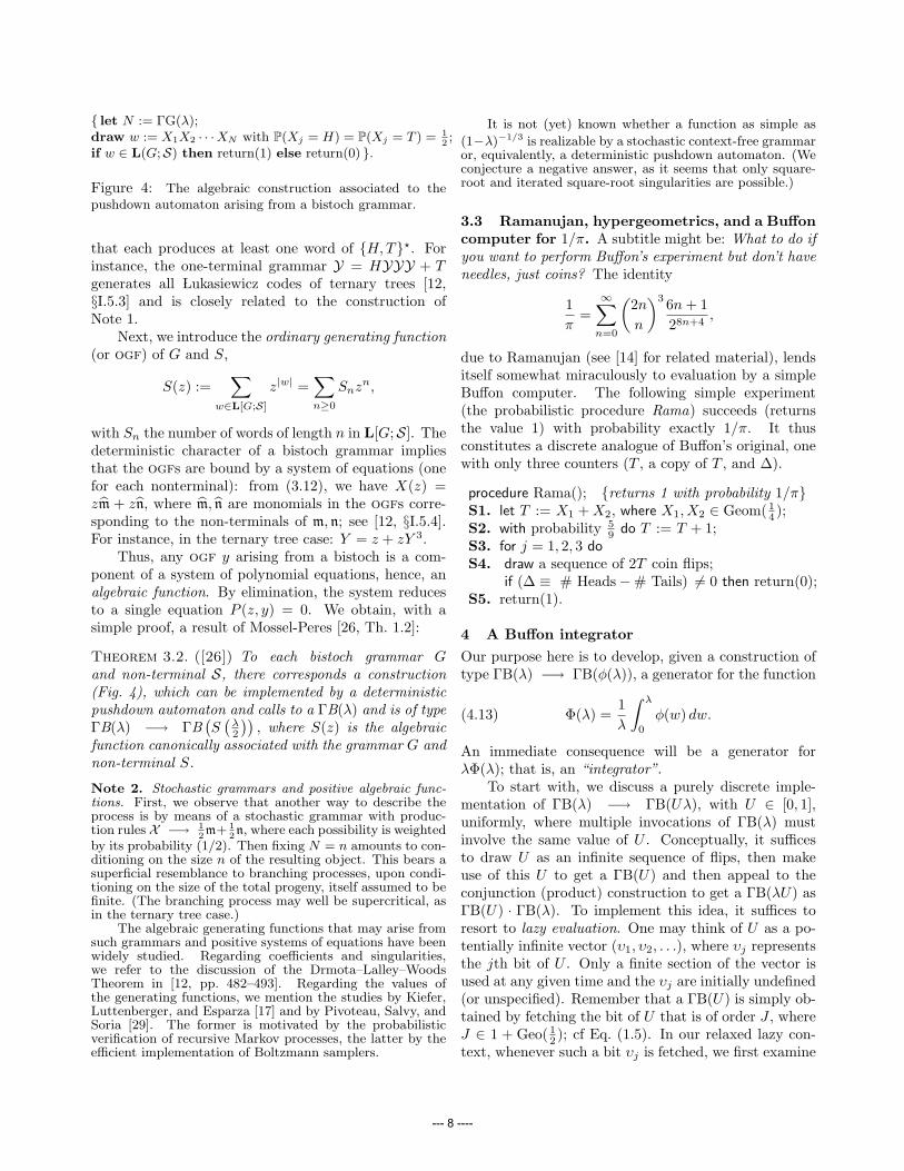
due to Ramanujan (see [14] for related material), lendsitself somewhat miraculously to evaluation by a simpleBuffon computer. The following simple experiment(the probabilistic procedure Rama) succeeds (returnsthe value 1) with probability exactly 1/π. It thusconstitutes a discrete analogue of Buffon’s original, onewith only three counters (T , a copy of T , and ∆).

procedure Rama(); {returns 1 with probability 1/π}S1. let T := X1 +X2, where X1, X2 ∈ Geom(1

4 );S2. with probability 5

9 do T := T + 1;S3. for j = 1, 2, 3 doS4. draw a sequence of 2T coin flips;

if (∆ ≡ # Heads−# Tails) 6= 0 then return(0);S5. return(1).

4 A Buffon integrator

Our purpose here is to develop, given a construction oftype ΓB(λ) −→ ΓB(φ(λ)), a generator for the function

Φ(λ) =1λ

∫ λ

0

φ(w) dw.(4.13)

An immediate consequence will be a generator forλΦ(λ); that is, an “integrator”.

To start with, we discuss a purely discrete imple-mentation of ΓB(λ) −→ ΓB(Uλ), with U ∈ [0, 1],uniformly, where multiple invocations of ΓB(λ) mustinvolve the same value of U . Conceptually, it sufficesto draw U as an infinite sequence of flips, then makeuse of this U to get a ΓB(U) and then appeal to theconjunction (product) construction to get a ΓB(λU) asΓB(U) · ΓB(λ). To implement this idea, it suffices toresort to lazy evaluation. One may think of U as a po-tentially infinite vector (υ1, υ2, . . .), where υj representsthe jth bit of U . Only a finite section of the vector isused at any given time and the υj are initially undefined(or unspecified). Remember that a ΓB(U) is simply ob-tained by fetching the bit of U that is of order J , whereJ ∈ 1 + Geo( 1

2 ); cf Eq. (1.5). In our relaxed lazy con-text, whenever such a bit υj is fetched, we first examine

--- 8 ----

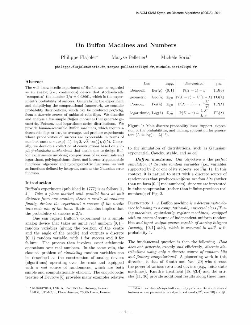
U =

11

20

30

50

61n nn

nn=

???10?001

9 :8 :7 :6 :5 :4 :3 :2 :1 :

⇐= J

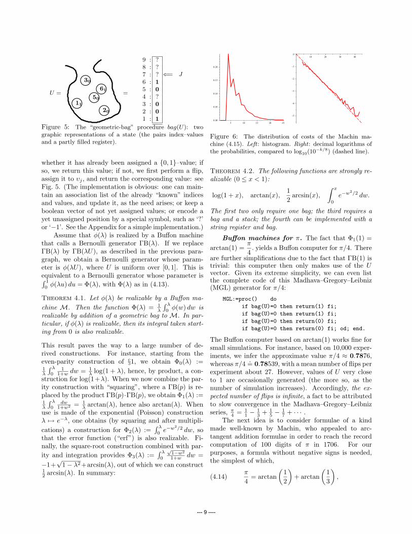
Figure 5: The “geometric-bag” procedure bag(U): twographic representations of a state (the pairs index–valuesand a partly filled register).

whether it has already been assigned a {0, 1}–value; ifso, we return this value; if not, we first perform a flip,assign it to υj , and return the corresponding value: seeFig. 5. (The implementation is obvious: one can main-tain an association list of the already “known” indicesand values, and update it, as the need arises; or keep aboolean vector of not yet assigned values; or encode ayet unassigned position by a special symbol, such as ‘?’or ‘−1’. See the Appendix for a simple implementation.)

Assume that φ(λ) is realized by a Buffon machinethat calls a Bernoulli generator ΓB(λ). If we replaceΓB(λ) by ΓB(λU), as described in the previous para-graph, we obtain a Bernoulli generator whose param-eter is φ(λU), where U is uniform over [0, 1]. This isequivalent to a Bernoulli generator whose parameter is∫ 1

0φ(λu) du = Φ(λ), with Φ(λ) as in (4.13).

Theorem 4.1. Let φ(λ) be realizable by a Buffon ma-chine M. Then the function Φ(λ) = 1

λ

∫ λ

0φ(w) dw is

realizable by addition of a geometric bag to M. In par-ticular, if φ(λ) is realizable, then its integral taken start-ing from 0 is also realizable.

This result paves the way to a large number of de-rived constructions. For instance, starting from theeven-parity construction of §1, we obtain Φ0(λ) :=1λ

∫ λ

01

1+w dw = 1λ log(1 + λ), hence, by product, a con-

struction for log(1+λ). When we now combine the par-ity construction with “squaring”, where a ΓB(p) is re-placed by the product ΓB(p)·ΓB(p), we obtain Φ1(λ) :=1λ

∫ λ

0dw

1+w2 = 1λ arctan(λ), hence also arctan(λ). When

use is made of the exponential (Poisson) constructionλ 7→ e−λ, one obtains (by squaring and after multipli-cations) a construction for Φ2(λ) :=

∫ λ

0e−w2/2 dw, so

that the error function (“erf”) is also realizable. Fi-nally, the square-root construction combined with par-ity and integration provides Φ3(λ) :=

∫ λ

0

√1−w2

1+w dw =−1+

√1− λ2 +arcsin(λ), out of which we can construct

12 arcsin(λ). In summary:

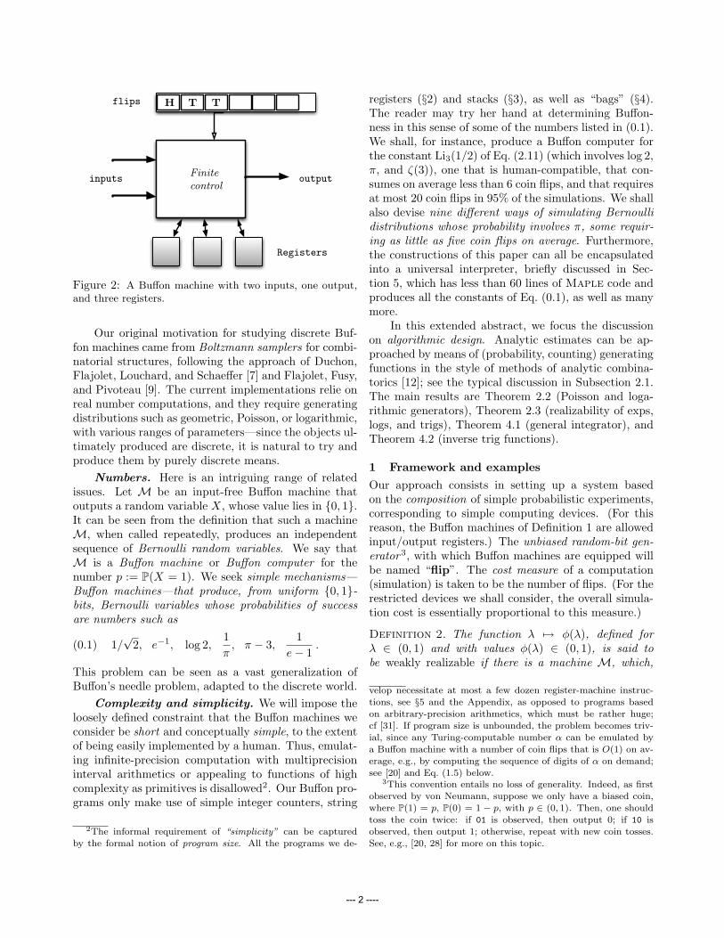
5 10 15 20 250.00

0.05

0.10

0.15

0.20

10 20 30 40

K5

K4

K3

K2

K1

0

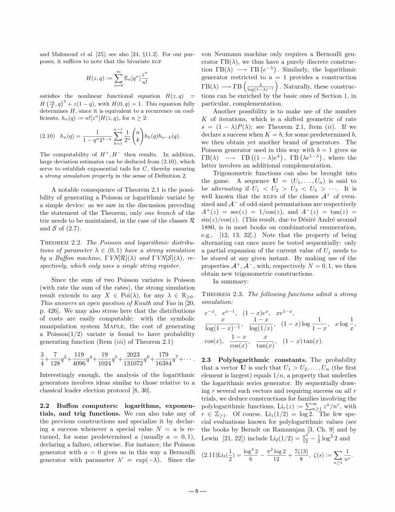
Figure 6: The distribution of costs of the Machin ma-chine (4.15). Left : histogram. Right : decimal logarithms ofthe probabilities, compared to log10(10−k/8) (dashed line).

Theorem 4.2. The following functions are strongly re-alizable (0 ≤ x < 1):

log(1 + x), arctan(x),12

arcsin(x),∫ x

0

e−w2/2 dw.

The first two only require one bag; the third requires abag and a stack; the fourth can be implemented with astring register and bag.

Buffon machines for π. The fact that Φ1(1) =arctan(1) =

π

4. yields a Buffon computer for π/4. There

are further simplifications due to the fact that ΓB(1) istrivial: this computer then only makes use of the Uvector. Given its extreme simplicity, we can even listthe complete code of this Madhava–Gregory–Leibniz(MGL) generator for π/4:

MGL:=proc() do

if bag(U)=0 then return(1) fi;

if bag(U)=0 then return(1) fi;

if bag(U)=0 then return(0) fi;

if bag(U)=0 then return(0) fi; od; end.

The Buffon computer based on arctan(1) works fine forsmall simulations. For instance, based on 10,000 exper-iments, we infer the approximate value π/4 ≈ 0.7876,whereas π/4 .= 0.78539, with a mean number of flips perexperiment about 27. However, values of U very closeto 1 are occasionally generated (the more so, as thenumber of simulation increases). Accordingly, the ex-pected number of flips is infinite, a fact to be attributedto slow convergence in the Madhava–Gregory–Leibnizseries, π

4 = 11 −

13 + 1

5 −17 + · · · .

The next idea is to consider formulae of a kindmade well-known by Machin, who appealed to arc-tangent addition formulae in order to reach the recordcomputation of 100 digits of π in 1706. For ourpurposes, a formula without negative signs is needed,the simplest of which,

π

4= arctan

(12

)+ arctan

(13

),(4.14)

--- 9 ----

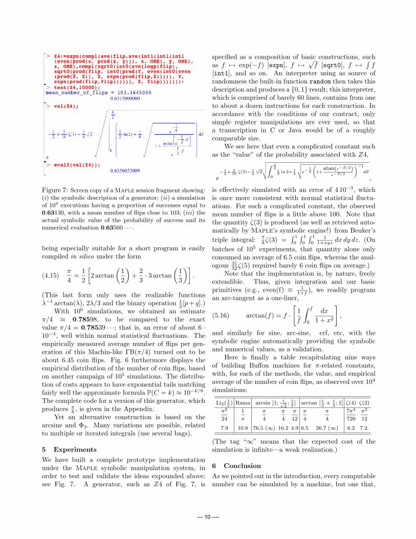
Figure 7: Screen copy of a Maple session fragment showing:(i) the symbolic description of a generator; (ii) a simulationof 104 executions having a proportion of successes equal to0.63130, with a mean number of flips close to 103; (iii) theactual symbolic value of the probability of success and itsnumerical evaluation 0.63560 · · · .

being especially suitable for a short program is easilycompiled in silico under the form

π

4=

12

[2 arctan

(12

)+

23· 3 arctan

(13

)].(4.15)

(This last form only uses the realizable functionsλ−1 arctan(λ), 2λ/3 and the binary operation 1

2 [p+ q].)With 106 simulations, we obtained an estimate

π/4 ≈ 0.78598, to be compared to the exactvalue π/4 = 0.78539 · · ·; that is, an error of about 6 ·10−4, well within normal statistical fluctuations. Theempirically measured average number of flips per gen-eration of this Machin-like ΓB(π/4) turned out to beabout 6.45 coin flips. Fig. 6 furthermore displays theempirical distribution of the number of coin flips, basedon another campaign of 105 simulations. The distribu-tion of costs appears to have exponential tails matchingfairly well the approximate formula P(C = k) ≈ 10−k/8.The complete code for a version of this generator, whichproduces π

8 , is given in the Appendix.Yet an alternative construction is based on the

arcsine and Φ3. Many variations are possible, relatedto multiple or iterated integrals (use several bags).

5 Experiments

We have built a complete prototype implementationunder the Maple symbolic manipulation system, inorder to test and validate the ideas expounded above;see Fig. 7. A generator, such as Z4 of Fig. 7, is

specified as a composition of basic constructions, suchas f 7→ exp(−f) [expn], f 7→

√f [sqrt0], f 7→

∫f

[int1], and so on. An interpreter using as source ofrandomness the built-in function random then takes thisdescription and produces a {0, 1} result; this interpreter,which is comprised of barely 60 lines, contains from oneto about a dozen instructions for each construction. Inaccordance with the conditions of our contract, onlysimple register manipulations are ever used, so thata transcription in C or Java would be of a roughlycomparable size.

We see here that even a complicated constant suchas the “value” of the probability associated with Z4,

e− 1

2+ 316 ζ(3)− 1

4√

2

vuuutZ 12

0

12 ln 2+ 1

4

vuute− 1

4

1+

atan(e−Z/2)e−Z/2

!−1

dZ

,

is effectively simulated with an error of 4 10−3, whichis once more consistent with normal statistical fluctu-ations. For such a complicated constant, the observedmean number of flips is a little above 100. Note thatthe quantity ζ(3) is produced (as well as retrieved auto-matically by Maple’s symbolic engine!) from Beuker’striple integral: 7

8ζ(3) =∫ 1

0

∫ 1

0

∫ 1

01

1+xyz dx dy dz. (Onbatches of 105 experiments, that quantity alone onlyconsumed an average of 6.5 coin flips, whereas the anal-ogous 31

32ζ(5) required barely 6 coin flips on average.)Note that the implementation is, by nature, freely

extendible. Thus, given integration and our basicprimitives (e.g., even(f) ≡ 1

1+f ), we readily programan arc-tangent as a one-liner,

arctan(f) = f ·

[1f

∫ f

0

dx

1 + x2

],(5.16)

and similarly for sine, arc-sine, erf, etc, with thesymbolic engine automatically providing the symbolicand numerical values, as a validation.

Here is finally a table recapitulating nine waysof building Buffon machines for π-related constants,with, for each of the methods, the value, and empiricalaverage of the number of coin flips, as observed over 104

simulations:

Li2( 12) Rama arcsin [1; 1√

2; 12] arctan [ 1

2+ 1

3; 1] ζ(4) ζ(2)

π2

24

1

π

π

4

π

4

π

12

π

4

π

4

7π4

720

π2

12

7.9 10.8 76.5 (∞) 16.2 4.9 6.5 26.7 (∞) 6.2 7.2.

(The tag “∞” means that the expected cost of thesimulation is infinite—a weak realization.)

6 Conclusion

As we pointed out in the introduction, every computablenumber can be simulated by a machine, but one that,

--- 10 ----

in general, will violate our charter of simplicity (as mea-sured, typically, by program size). Numbers accessibleto our framework seem not to include Euler’s constantγ.= 0.57721, and we must leave it as an open problem to

come up with a “natural” experiment, whose probabil-ity of success is γ. Perhaps the difficulty of the problemlies in the absence of a simple “positive” expression thatcould be compiled into a correspondingly simple Buffongenerator. By contrast, exotic numbers, such as π−1/π

or e− sin(1/√

7) are easily simulated. . .On another note, we have not considered the gen-

eration of continuous random variables X, specified bya distribution function F (x) = P(X ≤ x). Von Neu-mann’s original algorithm for an exponential variate be-longs to this paradigm. In this case, the bits of X areobtained by a short computation of O(1) initial bits,continued by the production of an infinite flow of uni-form random bits. This theme is thoroughly exploredby Knuth and Yao in [20]. It would be of obvious inter-est to be able to hybridize the von Neumann-Knuth-Yaogenerators of continuous distributions with our Buffoncomputers for discrete distributions. Interestingly, thefact that the Gaussian error function, albeit restrictedto the interval (0, 1), is realizable by Buffon machinessuggests the possibility of a totally discrete generatorfor a (standard) normal variate.

The present work is excellently summarized byKeane and O’Brien’s vivid expression of “Bernoulli fac-tory” [16]. It was initially approached with a purelytheoretical goal. It then came as a surprise that a pri-ori stringent theoretical requirements—those of perfectgeneration, discreteness of the random source, and sim-plicity of the mechanisms—could lead to computation-ally efficient algorithms. We have indeed seen manycases, from Bernoulli to logarithmic and Poisson gener-ators, where short programs and the execution of just afew dozen instructions suffice!Acknowledgements. This work was supported by theFrench ANR Projects Gamma, Boole, and Magnum. Theauthors are grateful to the referees of SODA-2011 for theirperceptive and encouraging comments.

References

[1] Badger, L. Lazzarini’s lucky approximation of π.Mathematics Magazine 67, 2 (1994), 83–91.

[2] Bailey, D., Borwein, P., and Plouffe, S. Onthe rapid computation of various polylogarithmic con-stants. Mathematics of Computation 66, 218 (1997),903–913.

[3] Berndt, B. C. Ramanujan’s Notebooks, Part I.Springer Verlag, 1985.

[4] Buffon, Comte de. Essai d’arithmetique morale. InHistoire Naturelle, generale et particuliere. Servant de

suite a l’Histoire Naturelle de l’Homme. Supplement,Tome Quatrieme. Imprimerie Royale, Paris, 1749–1789. Text available at gallica.bnf.fr. (Buffon’sneedle experiment is described on pp. 95–105.).

[5] Clement, J., Flajolet, P., and Vallee, B. Dy-namical sources in information theory: A general anal-ysis of trie structures. Algorithmica 29, 1/2 (2001),307–369.

[6] Devroye, L. Non-Uniform Random Variate Genera-tion. Springer Verlag, 1986.

[7] Duchon, P., Flajolet, P., Louchard, G., andSchaeffer, G. Boltzmann samplers for the randomgeneration of combinatorial structures. Combinatorics,Probability and Computing 13, 4–5 (2004), 577–625.Special issue on Analysis of Algorithms.

[8] Fill, J. A., Mahmoud, H. M., and Szpankowski,W. On the distribution for the duration of a random-ized leader election algorithm. The Annals of AppliedProbability 6, 4 (1996), 1260–1283.

[9] Flajolet, P., Fusy, E., and Pivoteau, C. Boltz-mann sampling of unlabelled structures. In Proceed-ings of the Ninth Workshop on Algorithm Engineeringand Experiments and the Fourth Workshop on AnalyticAlgorithmics and Combinatorics (2007), D. A. et al.,Ed., SIAM Press, pp. 201–211. Proceedings of the NewOrleans Conference.

[10] Flajolet, P., Gourdon, X., and Dumas, P. Mellintransforms and asymptotics: Harmonic sums. Theo-retical Computer Science 144, 1–2 (June 1995), 3–58.

[11] Flajolet, P., and Saheb, N. The complexity of gen-erating an exponentially distributed variate. Journal ofAlgorithms 7 (1986), 463–488.

[12] Flajolet, P., and Sedgewick, R. Analytic Com-binatorics. Cambridge University Press, 2009. 824pages. Also available electronically from the authors’home pages.

[13] Goulden, I. P., and Jackson, D. M. CombinatorialEnumeration. John Wiley, New York, 1983.

[14] Guillera, J. A new method to obtain series for 1/πand 1/π2. Experimental Mathematics 15, 1 (2006), 83–89.

[15] Jacquet, P., and Regnier, M. Trie partitioningprocess: Limiting distributions. In CAAP’86 (1986),P. Franchi-Zanetacchi, Ed., vol. 214 of Lecture Notesin Computer Science, pp. 196–210. Proceedings of the11th Colloquium on Trees in Algebra and Program-ming, Nice France, March 1986.

[16] Keane, M. S., and O’Brien, G. L. A Bernoullifactory. ACM Transactions on Modeling and ComputerSimulation (TOMACS) 4, 2 (1994), 213–219.

[17] Kiefer, S., Luttenberger, M., and Esparza, J.On the convergence of Newton’s method for monotonesystems of polynomial equations. In Symposium onTheory of Computing (STOC’07) (2007), ACM Press,pp. 217–226.

[18] Knuth, D. E. The Art of Computer Programming,3rd ed., vol. 2: Seminumerical Algorithms. Addison-Wesley, 1998.

--- 11 ----

[19] Knuth, D. E. The Art of Computer Programming,2nd ed., vol. 3: Sorting and Searching. Addison-Wesley, 1998.

[20] Knuth, D. E., and Yao, A. C. The complexityof nonuniform random number generation. In Al-gorithms and complexity (Proc. Sympos., Carnegie-Mellon Univ., Pittsburgh, Pa., 1976). Academic Press,New York, 1976, pp. 357–428.

[21] Lewin, L. Polylogarithms and Associated Functions.North Holland Publishing Company, 1981.

[22] Lewin, L., Ed. Structural Properties of Polyloga-rithms. American Mathematical Society, 1991.

[23] Mahmoud, H. M. Evolution of Random Search Trees.John Wiley, 1992.

[24] Mahmoud, H. M. Sorting, A Distribution Theory.Wiley-Interscience, New York, 2000.

[25] Mahmoud, H. M., Flajolet, P., Jacquet, P., andRegnier, M. Analytic variations on bucket selectionand sorting. Acta Informatica 36, 9-10 (2000), 735–760.

[26] Mossel, E., and Peres, Y. New coins from old:Computing with unknown bias. Combinatorica 25, 6(2005), 707–724.

[27] Nacu, S., and Peres, Y. Fast simulation of newcoins from old. The Annals of Applied Probability 15,1A (2005), 93–115.

[28] Peres, Y. Iterating Von Neumann’s procedure forextracting random bits. Annals of Statistics 20, 1(1992), 590–597.

[29] Pivoteau, C., Salvy, B., and Soria, M. Boltz-mann oracle for combinatorial systems. Discrete Math-ematics & Theoretical Computer Science Proceedings(2008). Mathematics and Computer Science Confer-ence. In press, 14 pages.

[30] Prodinger, H. How to select a loser. DiscreteMathematics 120 (1993), 149–159.

[31] Schonhage, A., Grotefeld, A., and Vetter, E.Fast Algorithms, A Multitape Turing Machine Im-plementation. Bibliographisches Institut, Mannheim,1994.

[32] Stanley, R. P. Enumerative Combinatorics, vol. II.Cambridge University Press, 1999.

[33] Szpankowski, W. Average-Case Analysis of Algo-rithms on Sequences. John Wiley, 2001.

[34] Vallee, B. Dynamical sources in information theory:Fundamental intervals and word prefixes. Algorithmica29, 1/2 (2001), 262–306.

[35] Wastlund, J. Functions arising by coin flipping.Technical Report, K.T.H, Stockholm, 1999.

[36] Yao, A. C. Contex-free grammars and random num-ber generation. In Combinatorial Algorithms on Words(1985), A. Apostolico and Z. Galil, Eds., vol. 12of NATO Advance Science Institute Series. SeriesF: Computer and Systems Sciences, Springer Verlag,pp. 357–361.

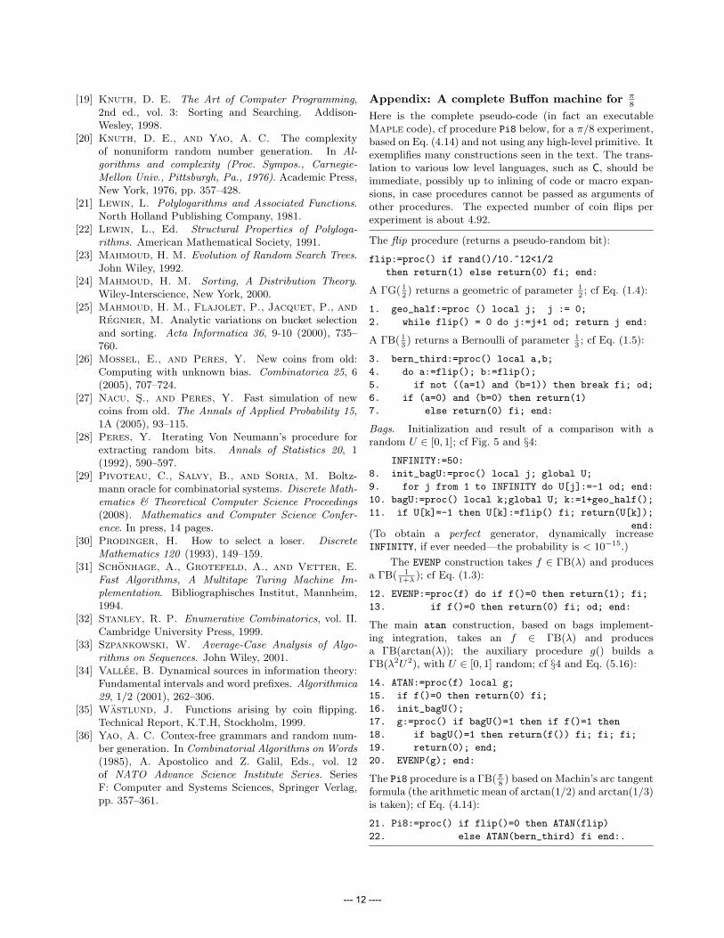
Appendix: A complete Buffon machine for π8

Here is the complete pseudo-code (in fact an executableMaple code), cf procedure Pi8 below, for a π/8 experiment,based on Eq. (4.14) and not using any high-level primitive. Itexemplifies many constructions seen in the text. The trans-lation to various low level languages, such as C, should beimmediate, possibly up to inlining of code or macro expan-sions, in case procedures cannot be passed as arguments ofother procedures. The expected number of coin flips perexperiment is about 4.92.

The flip procedure (returns a pseudo-random bit):

flip:=proc() if rand()/10.^12<1/2

then return(1) else return(0) fi; end:

A ΓG( 12) returns a geometric of parameter 1

2; cf Eq. (1.4):

1. geo_half:=proc () local j; j := 0;

2. while flip() = 0 do j:=j+1 od; return j end:

A ΓB( 13) returns a Bernoulli of parameter 1

3; cf Eq. (1.5):

3. bern_third:=proc() local a,b;

4. do a:=flip(); b:=flip();

5. if not ((a=1) and (b=1)) then break fi; od;

6. if (a=0) and (b=0) then return(1)

7. else return(0) fi; end:

Bags. Initialization and result of a comparison with arandom U ∈ [0, 1]; cf Fig. 5 and §4:

INFINITY:=50:

8. init_bagU:=proc() local j; global U;

9. for j from 1 to INFINITY do U[j]:=-1 od; end:

10. bagU:=proc() local k;global U; k:=1+geo_half();

11. if U[k]=-1 then U[k]:=flip() fi; return(U[k]);

end:(To obtain a perfect generator, dynamically increaseINFINITY, if ever needed—the probability is < 10−15.)

The EVENP construction takes f ∈ ΓB(λ) and producesa ΓB( 1

1+λ); cf Eq. (1.3):

12. EVENP:=proc(f) do if f()=0 then return(1); fi;

13. if f()=0 then return(0) fi; od; end:

The main atan construction, based on bags implement-ing integration, takes an f ∈ ΓB(λ) and producesa ΓB(arctan(λ)); the auxiliary procedure g() builds aΓB(λ2U2), with U ∈ [0, 1] random; cf §4 and Eq. (5.16):

14. ATAN:=proc(f) local g;

15. if f()=0 then return(0) fi;

16. init_bagU();

17. g:=proc() if bagU()=1 then if f()=1 then

18. if bagU()=1 then return(f()) fi; fi; fi;

19. return(0); end;

20. EVENP(g); end:

The Pi8 procedure is a ΓB(π8) based on Machin’s arc tangent

formula (the arithmetic mean of arctan(1/2) and arctan(1/3)is taken); cf Eq. (4.14):

21. Pi8:=proc() if flip()=0 then ATAN(flip)

22. else ATAN(bern_third) fi end:.

--- 12 ----