Modal Analysis of MDOF Systems with Proportional Dampingrotorlab.tamu.edu/me617/HD 8 prop damped...
22
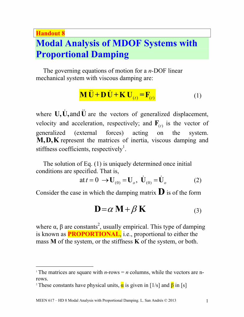
MEEN 617 – HD 8 Modal Analysis with Proportional Damping. L. San Andrés © 2013 1 Handout 8 Modal Analysis of MDOF Systems with Proportional Damping The governing equations of motion for a n-DOF linear mechanical system with viscous damping are: () () t t MU+DU+KU =F (1) where and U, U, U are the vectors of generalized displacement, velocity and acceleration, respectively; and () t F is the vector of generalized (external forces) acting on the system. M,D,K represent the matrices of inertia, viscous damping and stiffness coefficients, respectively 1 . The solution of Eq. (1) is uniquely determined once initial conditions are specified. That is, (0) (0) at 0 , o o t U U U U (2) Consider the case in which the damping matrix D is of the form D M K (3) where α, β are constants 2 , usually empirical. This type of damping is known as PROPORTIONAL, i.e., proportional to either the mass M of the system, or the stiffness K of the system, or both. 1 The matrices are square with n-rows = n columns, while the vectors are n- rows. 2 These constants have physical units, α is given in [1/s] and β in [s]
Transcript of Modal Analysis of MDOF Systems with Proportional Dampingrotorlab.tamu.edu/me617/HD 8 prop damped...
MEEN 617 – HD 8 Modal Analysis with Proportional Damping. L. San Andrés © 2013 1
Handout 8
Modal Analysis of MDOF Systems with Proportional Damping
The governing equations of motion for a n-DOF linear mechanical system with viscous damping are:
( ) ( )t tM U + DU +K U =F (1)
where andU,U, U are the vectors of generalized displacement,
velocity and acceleration, respectively; and ( )tF is the vector of
generalized (external forces) acting on the system. M,D,K represent the matrices of inertia, viscous damping and stiffness coefficients, respectively1.
The solution of Eq. (1) is uniquely determined once initial conditions are specified. That is,
(0) (0)at 0 ,o ot U U U U (2)
Consider the case in which the damping matrix D is of the form
D M K (3) where α, β are constants2, usually empirical. This type of damping is known as PROPORTIONAL, i.e., proportional to either the mass M of the system, or the stiffness K of the system, or both.
1 The matrices are square with n-rows = n columns, while the vectors are n-rows. 2 These constants have physical units, α is given in [1/s] and β in [s]
lsanandres
Rectangle
MEEN 617 – HD 8 Modal Analysis with Proportional Damping. L. San Andrés © 2013 2
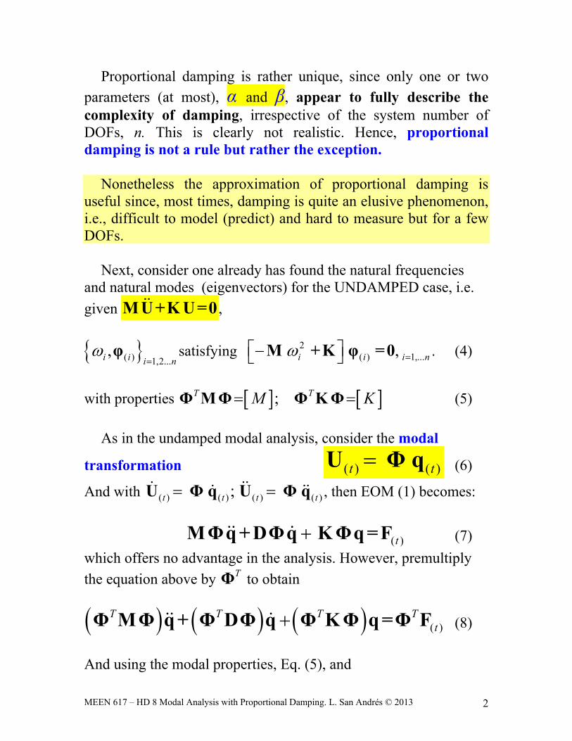
Proportional damping is rather unique, since only one or two
parameters (at most), α and β, appear to fully describe the complexity of damping, irrespective of the system number of DOFs, n. This is clearly not realistic. Hence, proportional damping is not a rule but rather the exception.
Nonetheless the approximation of proportional damping is
useful since, most times, damping is quite an elusive phenomenon, i.e., difficult to model (predict) and hard to measure but for a few DOFs.
Next, consider one already has found the natural frequencies
and natural modes (eigenvectors) for the UNDAMPED case, i.e.
given M U+K U=0 ,
( ) 1,2...,i i i n
φ satisfying 2( ) 1,...,i i i n M +K φ =0 . (4)
with properties ;T TM K Φ MΦ Φ KΦ (5)
As in the undamped modal analysis, consider the modal
transformation ( ) ( )t tU Φ q (6)
And with ( ) ( ) ( ) ( );t t t t U Φ q U Φ q , then EOM (1) becomes:
( )tMΦq + DΦq KΦq =F (7)
which offers no advantage in the analysis. However, premultiply
the equation above by TΦ to obtain
( )T T T T
tΦ MΦ q + Φ DΦ q Φ KΦ q =Φ F (8)
And using the modal properties, Eq. (5), and
MEEN 617 – HD 8 Modal Analysis with Proportional Damping. L. San Andrés © 2013 3
T T T T Φ DΦ Φ M K Φ Φ MΦ Φ KΦ
T M K D Φ DΦ (9)
i.e., [D] is a diagonal matrix known as proportional modal damping. Then Eq. (7) becomes
( )T
tM D K q + q q =Q Φ F (10)
Thus, the equations of motion are uncoupled in modal space, since [M], [D], and [K] are diagonal matrices. Eq. (10) is just a set of n-uncoupled ODEs. That is,
1 1 1 1 1 1 1
2 2 2 2 2 2 2
.....
n n n n n n n
M q D q K q Q
M q D q K q Q
M q D q K q Q
(11)
Or 1,2...,j j j j j j j j nM q D q K q Q (12)
Where j
jj
KMn and j j jD M K . Modal damping
ratios are also easily defined as
2 2j j j
j
j j j j
D M K
K M K M
; j=1,2,….n (13)
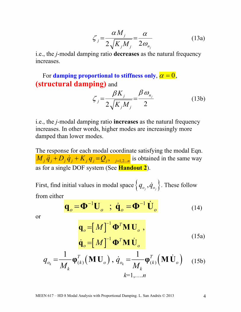
For damping proportional to mass only, 0 , and
MEEN 617 – HD 8 Modal Analysis with Proportional Damping. L. San Andrés © 2013 4
22j
jj
nj j
M
K M
(13a)
i.e., the j-modal damping ratio decreases as the natural frequency increases.
For damping proportional to stiffness only, 0 , (structural damping) and
22jnj
j
j j
K
K M
(13b)
i.e., the j-modal damping ratio increases as the natural frequency increases. In other words, higher modes are increasingly more damped than lower modes. The response for each modal coordinate satisfying the modal Eqn.
1,2...,j j j j j j j j nM q D q K q Q is obtained in the same way
as for a single DOF system (See Handout 2).
First, find initial values in modal space ,j jo oq q . These follow
from either 1 1;o o o o
q Φ U q Φ U (14) or
1
1
,To o
To o
M
M
q Φ M U
q Φ M U (15a)
( ) ( )
1 1,
k k
T To k o o k o
k k
q qM M
φ M U φ M U (15b)
k=1,….n
MEEN 617 – HD 8 Modal Analysis with Proportional Damping. L. San Andrés © 2013 5
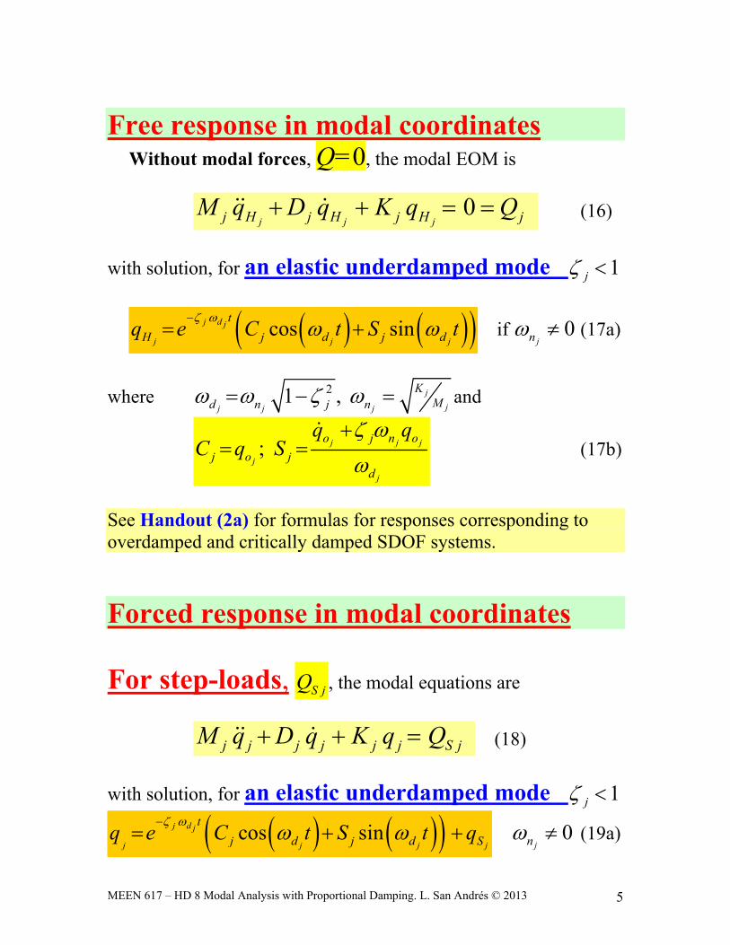
Free response in modal coordinates
Without modal forces, Q=0, the modal EOM is
0j j jj H j H j H jM q D q K q Q (16)
with solution, for an elastic underdamped mode 1j
cos sinj d j
j j j
t
H j d j dq e C t S t
if 0jn (17a)
where 21 , j
jj j j
KMd n j n and
; j j j
j
j
o j n o
j o jd
q qC q S
(17b)
See Handout (2a) for formulas for responses corresponding to overdamped and critically damped SDOF systems.
Forced response in modal coordinates
For step-loads, S jQ , the modal equations are
j j j j j j S jM q D q K q Q (18)
with solution, for an elastic underdamped mode 1j
cos sinj d j
j j j j
t
j d j d Sq e C t S t q
0jn (19a)
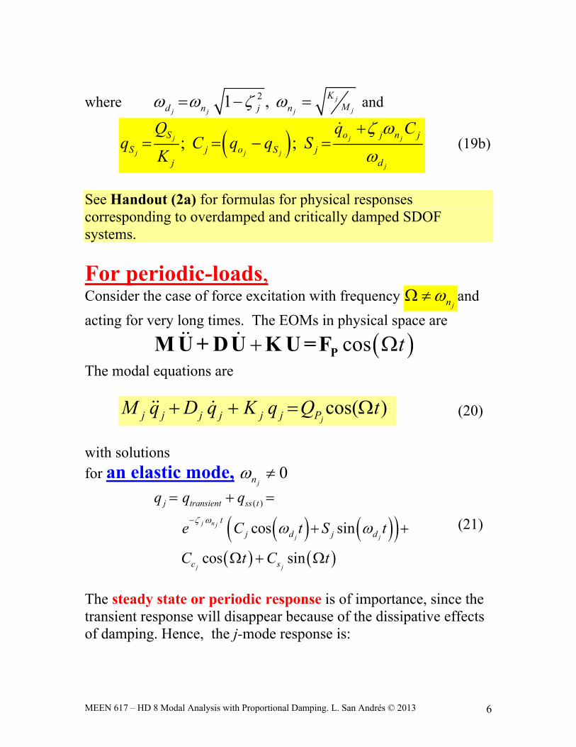
MEEN 617 – HD 8 Modal Analysis with Proportional Damping. L. San Andrés © 2013 6
where 21 , j
jj j j
KMd n j n and
; ;j j j
j j j
j
S o j n j
S j o S jj d
Q q Cq C q q S
K
(19b)
See Handout (2a) for formulas for physical responses corresponding to overdamped and critically damped SDOF systems.
For periodic-loads, Consider the case of force excitation with frequency
jn and
acting for very long times. The EOMs in physical space are
cos t PM U + DU K U =F
The modal equations are
cos( )jj j j j j j PM q D q K q Q t (20)
with solutions for an elastic mode, 0
jn
( )
cos sin
cos sin
j n j
j j
j j
j transient ss t
t
j d j d
c s
q q q
e C t S t
C t C t
(21)
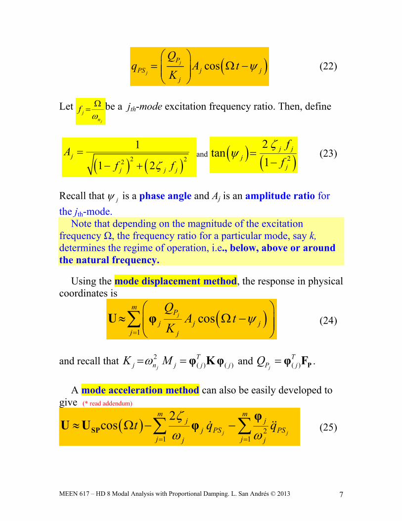
The steady state or periodic response is of importance, since the transient response will disappear because of the dissipative effects of damping. Hence, the j-mode response is:
MEEN 617 – HD 8 Modal Analysis with Proportional Damping. L. San Andrés © 2013 7
cosj
j
P
PS j jj
Qq A t
K
(22)
Let
j
jn
f
be a jth-mode excitation frequency ratio. Then, define
2 22
1
1 2 j
j j j
Af f
and 2
2tan
1j j
jj
f
f
(23)
Recall that j is a phase angle and Aj is an amplitude ratio for
the jth-mode. Note that depending on the magnitude of the excitation
frequency Ω, the frequency ratio for a particular mode, say k, determines the regime of operation, i.e., below, above or around the natural frequency.
Using the mode displacement method, the response in physical coordinates is
1
cosjm
P
j j jj j
QA t
K
U φ (24)
and recall that 2( ) ( )j
Tj n j j jK M φ Kφ and ( )j
TP jQ Pφ F .
A mode acceleration method can also be easily developed to
give (* read addendum)
21 1
2cos
j j
m mj j
j PS PSj jj j
t q q
SP
φU U φ (25)
MEEN 617 – HD 8 Modal Analysis with Proportional Damping. L. San Andrés © 2013 8
where 1SP pU K F . Note that the mode acceleration method
cannot be applied if there are any rigid body modes (K is singular)
Frequency response functions for damped MDOF systems. The steady state or periodic modal response for the j-mode is:
cosj
j
P
PS j jj
Qq A t
K
(22)
Or, taking the real part of the following complex number expression
j
j
P i tPS j
j
Qq H e
K
(26)
where 2
1
1 2 j
j j j
Hf i f
(27)
with 1i is the imaginary unit, and where j
jn
f
is the jth-
mode excitation frequency ratio. Then, recall from Eqs. (23)
2 22
1
1 2 j j
j j j
A Hf f
and argj jH (28)
Using the modal transformation, the periodic response UP in
physical coordinates is
MEEN 617 – HD 8 Modal Analysis with Proportional Damping. L. San Andrés © 2013 9
1
cosjn
P
j j jj j
QA t
K
PU φ (24)
or take the real part of the equation below
1 1
1
Tn nj i t
j j j jj j j
njT i t
j jj j
q H eK
He
K
PP
P
φ FU Φq φ φ
φ φ F
(29)
Now, the product ( )Tj j n n φ φ matrix . That is, define the
elements of the complex – frequency response matrix H as
, 2
1
1 2 p q
Tj j
p qj j j j
HK f i f
φ φ (30)
p,q =1,2…. n. The response in physical coordinates thus becomes:
i te P PU = H F (31)
or in component form,
, 1,2..1
;j r
ni t
P j r P j nr
U H F e
(32)
The components of the frequency response matrix H are determined numerically or experimentally. In any case, the components of H depend on the excitation frequency (Ω).
MEEN 617 – HD 8 Modal Analysis with Proportional Damping. L. San Andrés © 2013 10
Determining the elements of H seems laborious and (perhaps) its physical meaning remains elusive.
Direct Method to Find Frequency Responses in MDOF Systems
Nowadays, with fast computing power at our fingertips, the young engineer prefers to pursue a more direct approach, one known as brute force or direct approach. Recall that the equation of motion is
Or
cos
Re i t
t
e
P
P
M U + DU K U =F
M U + DU K U = F
(33)
Assume a periodic solution of the form i te
PU = V (34)
where PV is a vector in the complex domain. Substitution of Eq. (34) into Eq. (33) gives
2i P PK D M V F (35)
Define at each excitation frequency the complex impedance (dynamic stiffness) matrix as:
2i DK K D M (36)
And find the vector of physical responses (amplitude and phase) as
1
P PDV K F (37)
MEEN 617 – HD 8 Modal Analysis with Proportional Damping. L. San Andrés © 2013 11
Sincereal imaginary
i P P PV V V , the physical response for each DOF
follows as:
1,2...
2 2
cos ;
; tan
r
P imaginaryr
r r r P realr
r P r r n
VP P real P imaginary r V
U V t
V V V
(38)
The direct method requires calculating the inverse of the
dynamic stiffness matrix at each excitation frequency. The computational effort to perform this task could be excessive but for systems with a few DOFs (n small).
Let: 2
= (3)
If M is invertable, then define A M 1 K (4)
and write Eq. (2) as: A = (5)
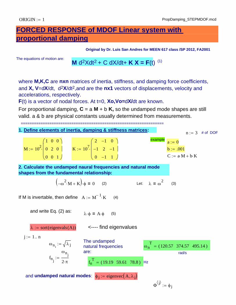
sort eigenvals A( )( ) <---- find eigenvalues
j 1 nThe undampednatural frequenciesare:
nj j n
T120.57 374.57 495.14( )
rad/sfnj
nj
2
fnT 19.19 59.61 78.8( ) Hz
and undamped natural modes: j eigenvec A j
j j
ORIGIN 1 PropDamping_STEPMDOF.mcd
FORCED RESPONSE of MDOF Linear system with proportional damping
Original by Dr. Luis San Andres for MEEN 617 class /SP 2012, FA2001
The equations of motion are:(1)M d2Xdt2 + C dX/dt+ K X = F(t)
where M,K,C are nxn matrices of inertia, stiffness, and damping force coefficients,and X, V=dX/dt, d2X/dt2,and are the nx1 vectors of displacements, velocity and accelerations, respectively. F(t) is a vector of nodal forces. At t=0, Xo,Vo=dX/dt are known.
For proportional damping, C = a M + b K, so the undamped mode shapes are still valid. a & b are physical constants usually determined from measurements.
=================================================================
1. Define elements of inertia, damping & stiffness matrices: n 3 # of DOF
example a 0M 102
1
0
0
0
2
0
0
0
1
K 1072
1
0
1
2
1
0
1
1
b .001C a M b K
2. Calculate the undamped naural frequencies and natural mode shapes from the fundamental relationship:
2
M K 0= (2)
dqo
dtMm
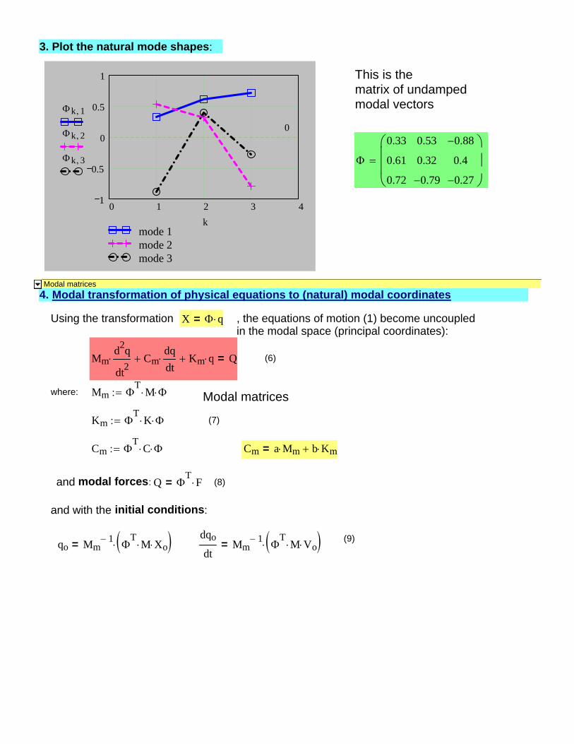
1 T
M Vo =qo Mm1
TM Xo =
(9)
and with the initial conditions:
(8)Q T
F=and modal forces:
Cm a Mm b Km=Cm T
C
(7)Km T
K
Modal matricesMm T
M where:
(6)Mmd2q
dt2 Cm
dqdt
Km q Q=
, the equations of motion (1) become uncoupled in the modal space (principal coordinates):
X q=Using the transformation
4. Modal transformation of physical equations to (natural) modal coordinatesModal matrices
0.33
0.61
0.72
0.53
0.32
0.79
0.88
0.4
0.27
This is thematrix of undampedmodal vectors
0 1 2 3 41
0.5
0
0.5
1
mode 1mode 2mode 3
0
k 1
k 2
k 3
k
3. Plot the natural mode shapes:
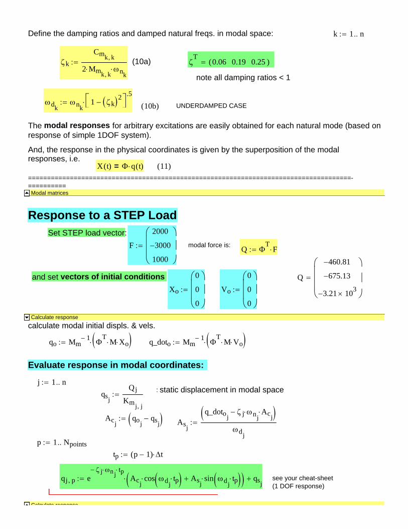
Q T
F
and set vectors of initial conditions Q
460.81
675.13
3.21 103
Xo
0
0
0
Vo
0
0
0
Calculate response
calculate modal initial displs. & vels.
qo Mm1
TM Xo q_doto Mm
1 T
M Vo
Evaluate response in modal coordinates:
j 1 n: static displacement in modal spaceqsj
Qj
Kmj j
Acjqoj
qsj Asj
q_dotoj j nj Acj
dj
p 1 Npointstp p 1( ) t
qj p e j nj tp
Acjcos dj
tp Asjsin dj
tp qsj see your cheat-sheet
(1 DOF response)
Calculate response
Define the damping ratios and damped natural freqs. in modal space: k 1 n
kCmk k
2 Mmk k nk
(10a)
T0.06 0.19 0.25( )
note all damping ratios < 1
dknk
1 k 2
.5 10b( ) UNDERDAMPED CASE
The modal responses for arbitrary excitations are easily obtained for each natural mode (based on response of simple 1DOF system).
And, the response in the physical coordinates is given by the superposition of the modal responses, i.e.
X t( ) q t( )= 11( )=====================================================================================-==========Modal matrices
Response to a STEP LoadSet STEP load vector:
F
2000
3000
1000
modal force is:
lsanandres
Rectangle
lsanandres
Rectangle
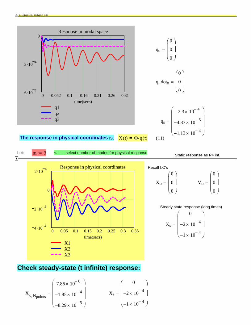
Xs
0
2 10 4
1 10 4
Xs Npoints
7.86 10 6
1.85 10 4
8.29 10 5
Check steady-state (t infinite) response:
Xs
0
2 10 4
1 10 4
Steady state response (long times)
Vo
0
0
0
Xo
0
0
0
Recall I.C's
0 0.05 0.1 0.15 0.2 0.25 0.3 0.354 10 4
2 10 4
0
2 10 4
X1X2X3
Response in physical coordinates
time(secs)
Static response as t-> inf.<------ select number of modes for physical responsem 3Let:
11( )X t( ) q t( )=The response in physical coordinates is:
qs
2.3 10 4
4.37 10 5
1.13 10 4
q_doto
0
0
0
qo
0
0
0
0 0.052 0.1 0.16 0.21 0.26 0.316 10 4
3 10 4
0
q1q2q3
Response in modal space
time(secs)
Calculate response
T
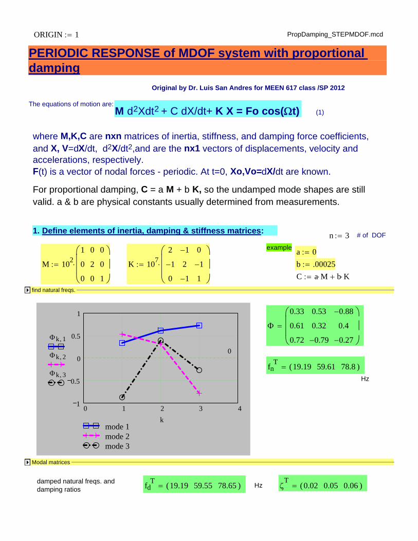
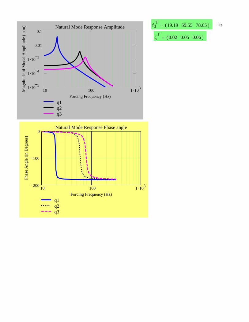
0.02 0.05 0.06( )HzfdT 19.19 59.55 78.65( )damped natural freqs. and
damping ratios
Modal matrices
Hz
fnT 19.19 59.61 78.8( )
0.33
0.61
0.72
0.53
0.32
0.79
0.88
0.4
0.27
0 1 2 3 41
0.5
0
0.5
1
mode 1mode 2mode 3
0
k 1
k 2
k 3
k
find natural freqs.
C a M b Kb .00025K 107
2
1
0
1
2
1
0
1
1
M 1021
0
0
0
2
0
0
0
1
a 0example
# of DOFn 31. Define elements of inertia, damping & stiffness matrices:
For proportional damping, C = a M + b K, so the undamped mode shapes are still valid. a & b are physical constants usually determined from measurements.
where M,K,C are nxn matrices of inertia, stiffness, and damping force coefficients,and X, V=dX/dt, d2X/dt2,and are the nx1 vectors of displacements, velocity and accelerations, respectively. F(t) is a vector of nodal forces - periodic. At t=0, Xo,Vo=dX/dt are known.
(1)M d2Xdt2 + C dX/dt+ K X = Fo cos(t) The equations of motion are:
Original by Dr. Luis San Andres for MEEN 617 class /SP 2012
PERIODIC RESPONSE of MDOF system with proportional damping
PropDamping_STEPMDOF.mcdORIGIN 1
Calculate response
See your cheat-sheet(1 DOF response)
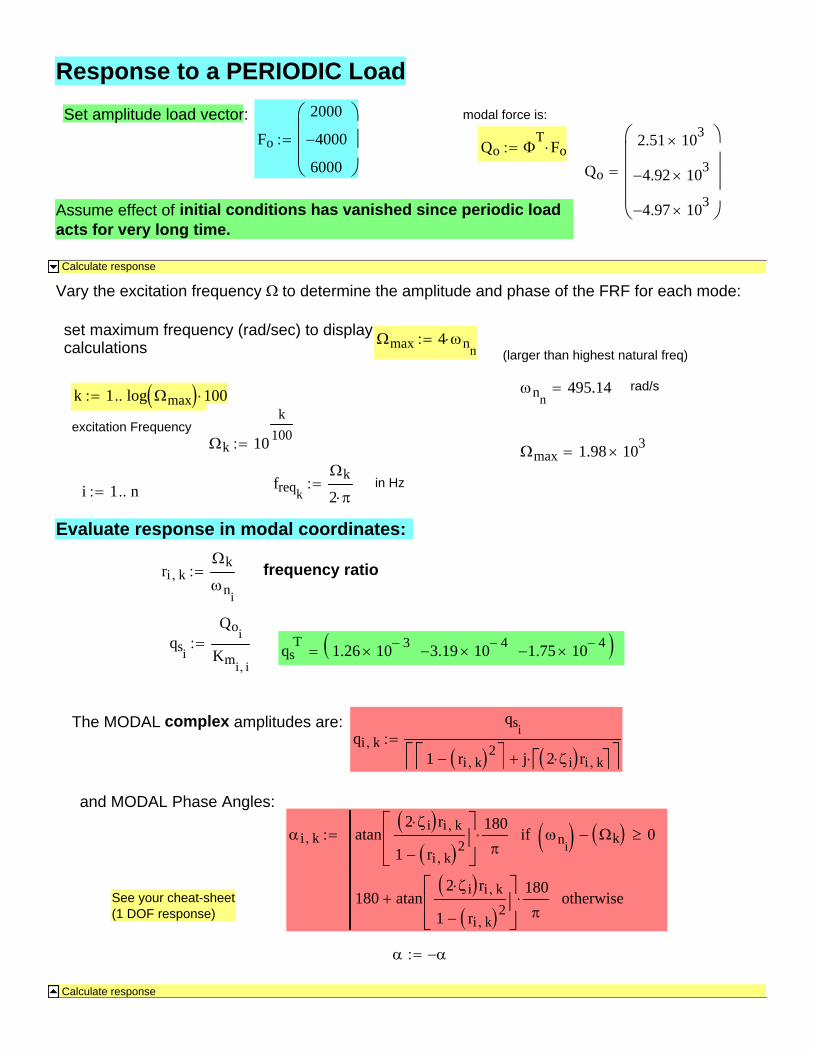
i k atan2 i ri k
1 ri k 2
180
ni k 0if
180 atan2 i ri k
1 ri k 2
180
otherwise
and MODAL Phase Angles:
qi k
qsi
1 ri k 2 j 2 i ri k
The MODAL complex amplitudes are:
qsT 1.26 10 3 3.19 10 4 1.75 10 4 qsi
Qoi
Kmi i
frequency ratiori kk
ni
Evaluate response in modal coordinates:
i 1 n in Hzfreqk
k
2
max 1.98 103
Response to a PERIODIC Load
Set amplitude load vector: modal force is:
Fo
2000
4000
6000
Qo T
FoQo
2.51 103
4.92 103
4.97 103
Assume effect of initial conditions has vanished since periodic load acts for very long time.
Calculate response
Vary the excitation frequency to determine the amplitude and phase of the FRF for each mode:
set maximum frequency (rad/sec) to display calculations
max 4 nn
(larger than highest natural freq)
rad/snn495.14k 1 log max 100
excitation Frequencyk 10
k100
lsanandres
Rectangle
10 100 1 1031 10 5
1 10 4
1 10 3
0.01
0.1
q1q2q3
Natural Mode Response Amplitude
Forcing Frequency (Hz)
Mag
nitu
de o
f Mod
al A
mpl
itude
(in
m) fd
T 19.19 59.55 78.65( ) Hz
T
0.02 0.05 0.06( )
10 100 1 103200
100
0
q1q2q3
Natural Mode Response Phase angle
Forcing Frequency (Hz)
Phas
e A
ngle
(in
Deg
rees
)
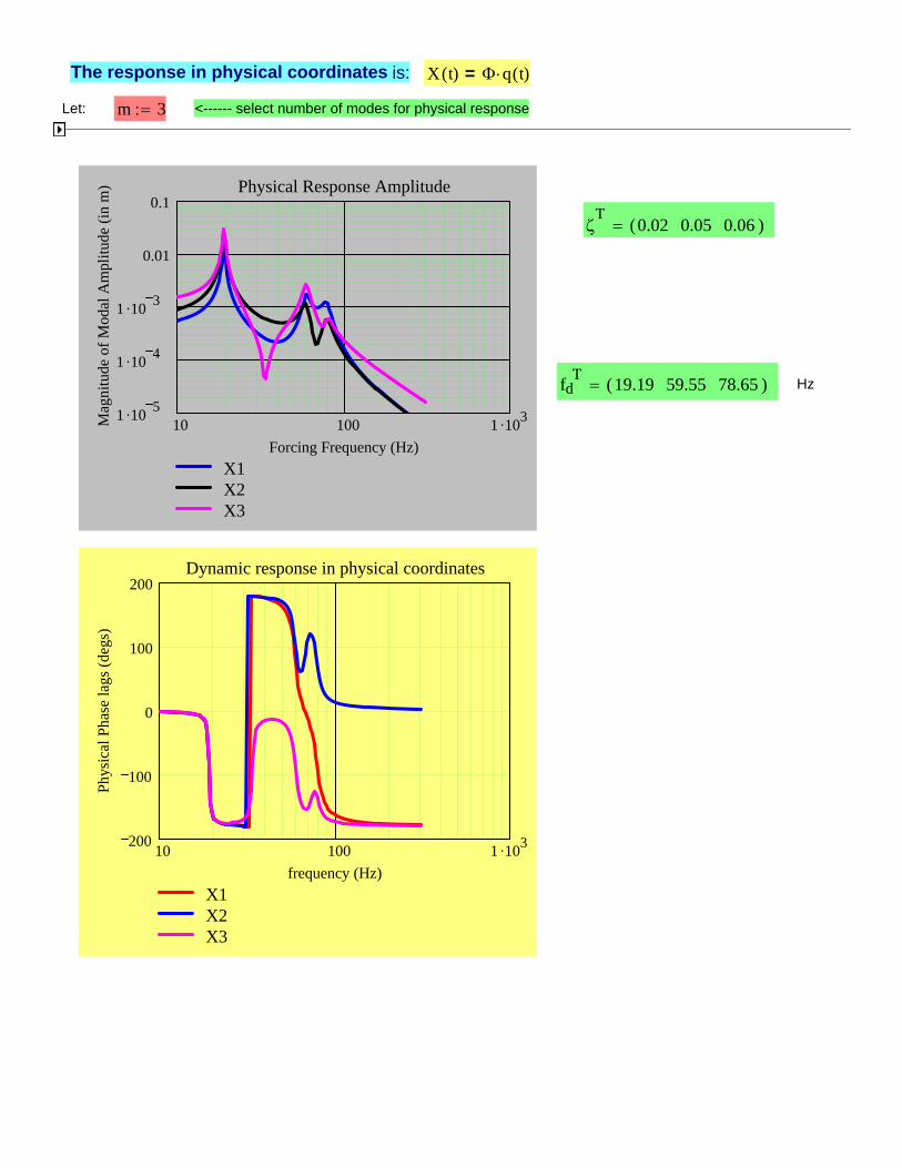
The response in physical coordinates is: X t( ) q t( )=
Let: m 3 <------ select number of modes for physical response
10 100 1 1031 10 5
1 10 4
1 10 3
0.01
0.1
X1X2X3
Physical Response Amplitude
Forcing Frequency (Hz)
Mag
nitu
de o
f Mod
al A
mpl
itude
(in
m)
T
0.02 0.05 0.06( )
fdT 19.19 59.55 78.65( ) Hz
10 100 1 103200
100
0
100
200
X1 X2X3
Dynamic response in physical coordinates
frequency (Hz)
Phys
ical
Pha
se la
gs (d
egs)
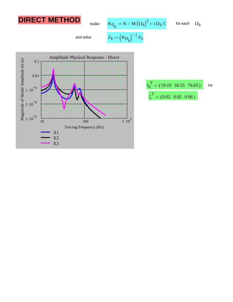
DIRECT METHOD make KDkK M k 2
i k C for each k
and solve Zk KDk 1 Fo
10 100 1 1031 10 5
1 10 4
1 10 3
0.01
0.1
X1X2X3
Amplitude Physical Response - Direct
Forcing Frequency (Hz)
Mag
nitu
de o
f Mod
al A
mpl
itude
(in
m)
fdT 19.19 59.55 78.65( ) Hz
T
0.02 0.05 0.06( )
lsanandres
Rectangle
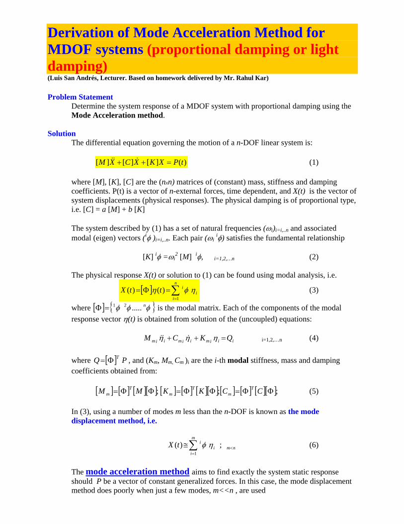
Derivation of Mode Acceleration Method for MDOF systems (proportional damping or light damping) (Luis San Andrés, Lecturer. Based on homework delivered by Mr. Rahul Kar)
Problem Statement
Determine the system response of a MDOF system with proportional damping using the Mode Acceleration method.
Solution The differential equation governing the motion of a n-DOF linear system is:
[ ] [ ] [ ] ( )M X C X K X P t+ + = (1) where [M], [K], [C] are the (nxn) matrices of (constant) mass, stiffness and damping coefficients. P(t) is a vector of n-external forces, time dependent, and X(t) is the vector of system displacements (physical responses). The physical damping is of proportional type, i.e. [C] = a [M] + b [K] The system described by (1) has a set of natural frequencies (ωi)i=i,..n and associated modal (eigen) vectors (iφ )i=i,..n. Each pair (ωi iφ) satisfies the fundamental relationship
[K] iφ =ωi2 [M]
iφ, i=1,2,…n (2) The physical response X(t) or solution to (1) can be found using modal analysis, i.e.
[ ] ∑=
=Φ=n
ii
ittX1
)()( ηφη (3)
where [ ] φφφ n.....21=Φ is the modal matrix. Each of the components of the modal response vector η(t) is obtained from solution of the (uncoupled) equations:
iiimiimiim QKCM =++ ηηη i=1,2,…n (4) where [ ] PQ TΦ= , and (Km, Mm, Cm )i are the i-th modal stiffness, mass and damping coefficients obtained from:
[ ] [ ] [ ][ ] [ ] [ ] [ ][ ] [ ] [ ] [ ][ ];;; ΦΦ=ΦΦ=ΦΦ= CCKKMM Tm
Tm
Tm (5)
In (3), using a number of modes m less than the n-DOF is known as the mode displacement method, i.e.
nm
m
ii
itX <=∑≅ ;)(
1
ηφ (6)
The mode acceleration method aims to find exactly the system static response should P be a vector of constant generalized forces. In this case, the mode displacement method does poorly when just a few modes, m<<n , are used
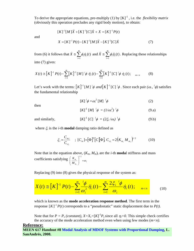
To derive the appropriate equations, pre-multiply (1) by [K]-1 , i.e. the flexibility matrix (obviously this operation precludes any rigid body motion), to obtain:
1 1 1[ ] [ ] [ ] [ ] [ ] ( )K M X K C X X K P t− − −+ + = and
1 1 1[ ] ( ) [ ] [ ] [ ] [ ]X K P t K M X K C X− − −= − − (7)
from (6) it follows that1
( )m
i ii
X tφη=
≅ ∑ and1
( )m
i ii
X tφη=
≅ ∑ . Replacing these relationships
into (7) gives:
[ ] [ ] [ ]∑∑=
<−
=
−− −−≅m
inmi
im
ii
i tCKtMKtPKtX1
1
1
11 ;)(][)(][)()( ηφηφ (8)
Let’s work with the terms: [ ] [ ] φφ ii CKandMK ][][ 11 −− . Since each pair (ωi , iφ) satisfies the fundamental relationship
[K] iφ =ωi2 [M]
iφ (2) then
[K]-1 [M] iφ = (1/ωi
2) iφ (9.a) and similarly, [K]-1 [C]
iφ = (2ξi /ωi) iφ (9.b) where ξi is the i-th modal damping ratio defined as
[ ] [ ][ ] ( ) 2/12,][;iii
i
mmcrT
mcr
imi MKCCC
CC
=ΦΦ==ξ (10)
Note that in the equation above, (Km, Mm)i are the i-th modal stiffness and mass coefficients satisfying
im
m
i
i
MK
ω=⎟⎟⎠
⎞⎜⎜⎝
⎛2/1
Replacing (9) into (8) gives the physical response of the system as:
[ ] ∑∑=
<=
− −−≅m
inmi
i
ii
m
ii
i
i
tttPKtX11
21 ;)(
2)()()( η
ωφξ
ηωφ
(10)
which is known as the mode acceleration response method. The first term in the response 1[ ] ( )K P t− corresponds to a “pseudostatic” static displacement due to P(t). Note that for P = Ps (constant), X=Xs=[K]-1Ps since all ηi=0. This simple check certifies the accuracy of the mode acceleration method even when using few modes (m<n).
Reference: MEEN 617 Handout #8 Modal Analysis of MDOF Systems with Proportional Damping, L. SanAndrés, 2008.


![The Fundamentals of Modal Testingliterature.cdn.keysight.com/litweb/pdf/5954-7957E.pdf · 2000. 9. 2. · MDOF impulse response/ free decay k1 k3 k2 k4 c1 c3 c2 4 m1 m2 m 3 [m]{x}](https://static.fdocument.org/doc/165x107/60d26ca59f186d32213cccdf/the-fundamentals-of-modal-2000-9-2-mdof-impulse-response-free-decay-k1-k3.jpg)
![A Fibrational Framework for Substructural and Modal ......A Judgemental Deconstruction of Modal Logic [Reed’09] Adjoint Logic with a 2-Category of Modes [L.Shulman’16] A Fibrational](https://static.fdocument.org/doc/165x107/600c830a7eb54a53f75f0b13/a-fibrational-framework-for-substructural-and-modal-a-judgemental-deconstruction.jpg)
![A Fibrational Framework for Substructural and Modal Logics ...dlicata.web.wesleyan.edu/pubs/lsr17multi/lsr17multi-ex.pdf · Shulman [2012], Shulman [2015] proposed using modal operators](https://static.fdocument.org/doc/165x107/5e845c463abf2542623a53a3/a-fibrational-framework-for-substructural-and-modal-logics-shulman-2012-shulman.jpg)