MACHINE LEARNING IN HIGHENERGY PHYSICSLECTURE #4

Alex Rogozhnikov, 2015

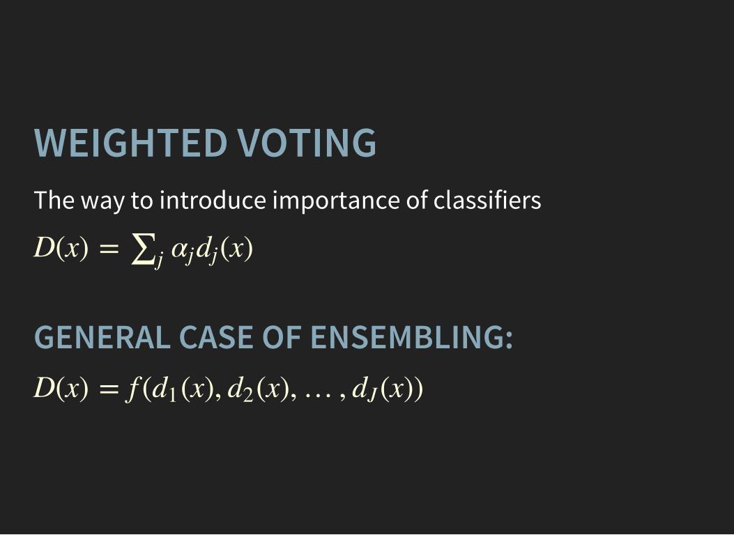
WEIGHTED VOTINGThe way to introduce importance of classifiers

D(x) = (x)*j αjdj

GENERAL CASE OF ENSEMBLING:D(x) = f ( (x), (x),… , (x))d1 d2 dJ

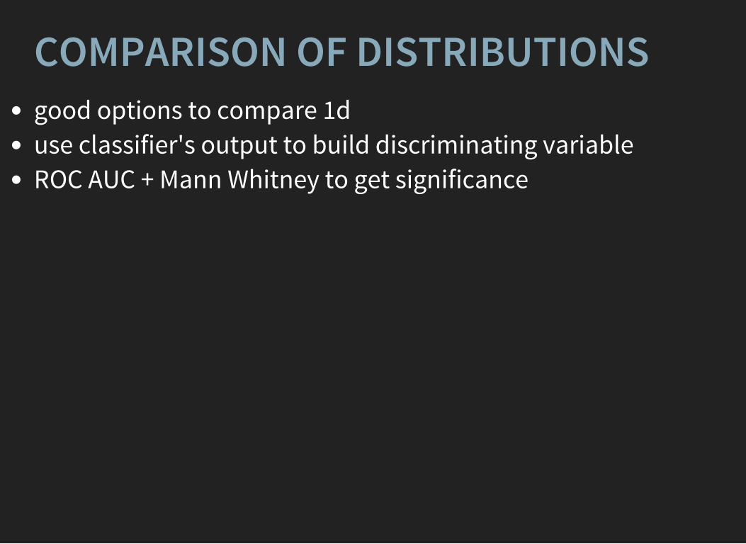
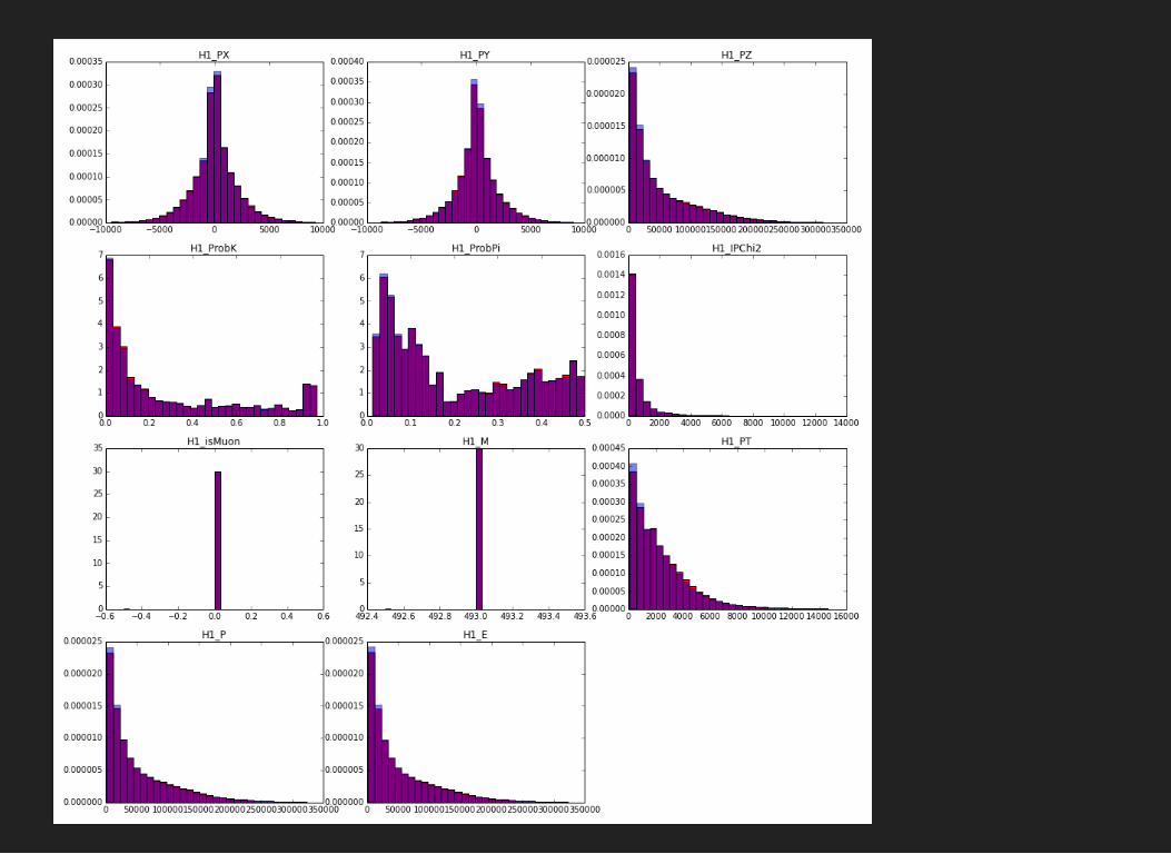
COMPARISON OF DISTRIBUTIONSgood options to compare 1duse classifier's output to build discriminating variableROC AUC + Mann Whitney to get significance

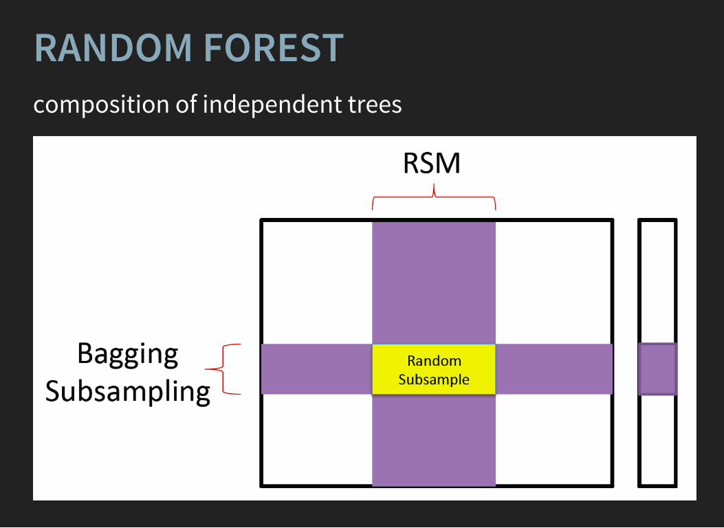
RANDOM FORESTcomposition of independent trees

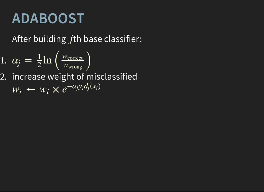
ADABOOSTAfter building th base classifier:j

1.

2. increase weight of misclassified

= ln ( )αj12

wcorrectwwrong

← ×wi wi e+ ( )αjyidj xi

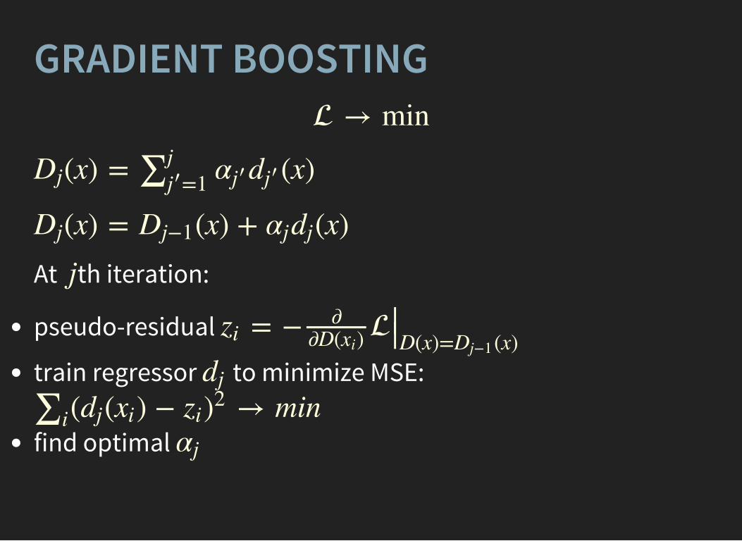
GRADIENT BOOSTING → min

(x) = (x)Dj *j=1j ′ αj ′ dj ′

(x) = (x) + (x)Dj Dj+1 αjdj

At th iteration:j

pseudo-residual

train regressor to minimize MSE:

find optimal

= + zi�

�D( )xi<<D(x)= (x)Dj+1

dj( ( ) + → min*i dj xi zi)2

αj

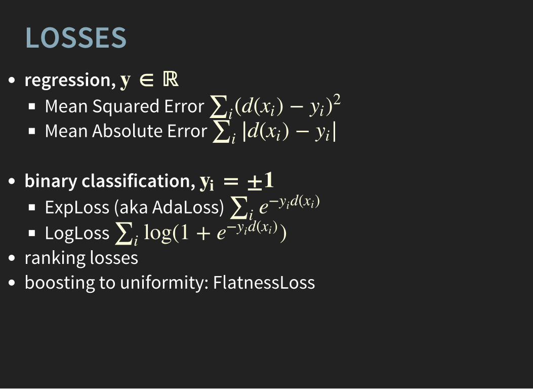
LOSSESregression,

Mean Squared Error Mean Absolute Error

binary classification, ExpLoss (aka AdaLoss) LogLoss

ranking lossesboosting to uniformity: FlatnessLoss

y ∈ ℝ(d( ) +*i xi yi)2

d( ) +*i << xi yi<<

= ±1yi*i e+ d( )yi xi

log(1 + )*i e+ d( )yi xi

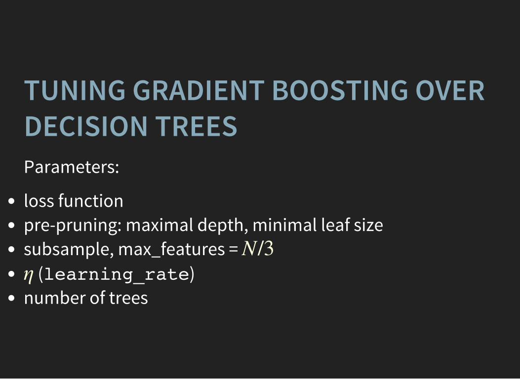
TUNING GRADIENT BOOSTING OVERDECISION TREESParameters:

loss functionpre-pruning: maximal depth, minimal leaf sizesubsample, max_features =

(learning_rate)number of trees

N/3η

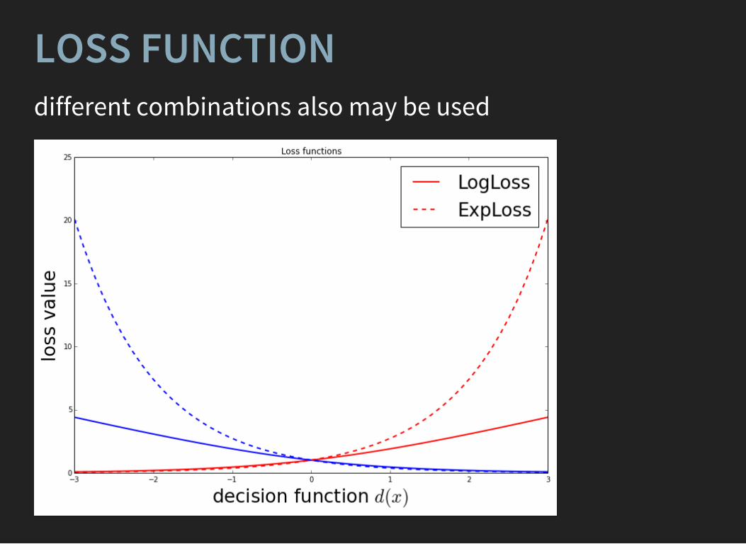
LOSS FUNCTIONdifferent combinations also may be used

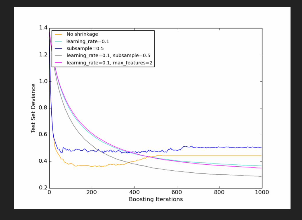
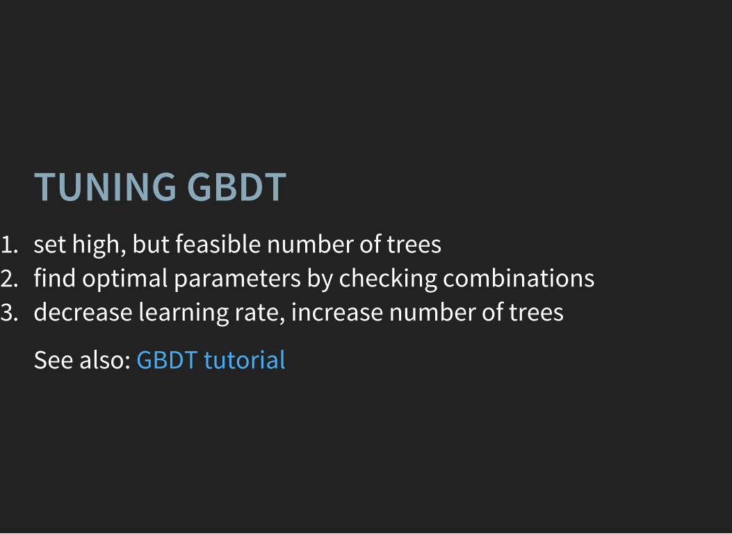
TUNING GBDT1. set high, but feasible number of trees2. find optimal parameters by checking combinations3. decrease learning rate, increase number of trees

See also: GBDT tutorial

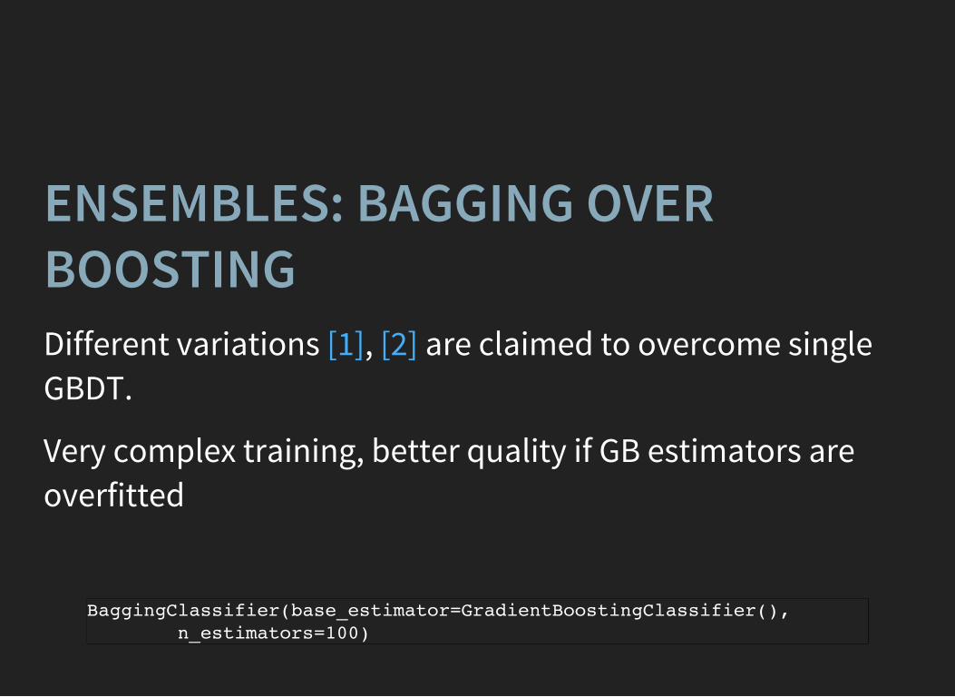
BaggingClassifier(base_estimator=GradientBoostingClassifier(), n_estimators=100)

ENSEMBLES: BAGGING OVERBOOSTINGDifferent variations , are claimed to overcome singleGBDT.

[1] [2]

Very complex training, better quality if GB estimators areoverfitted

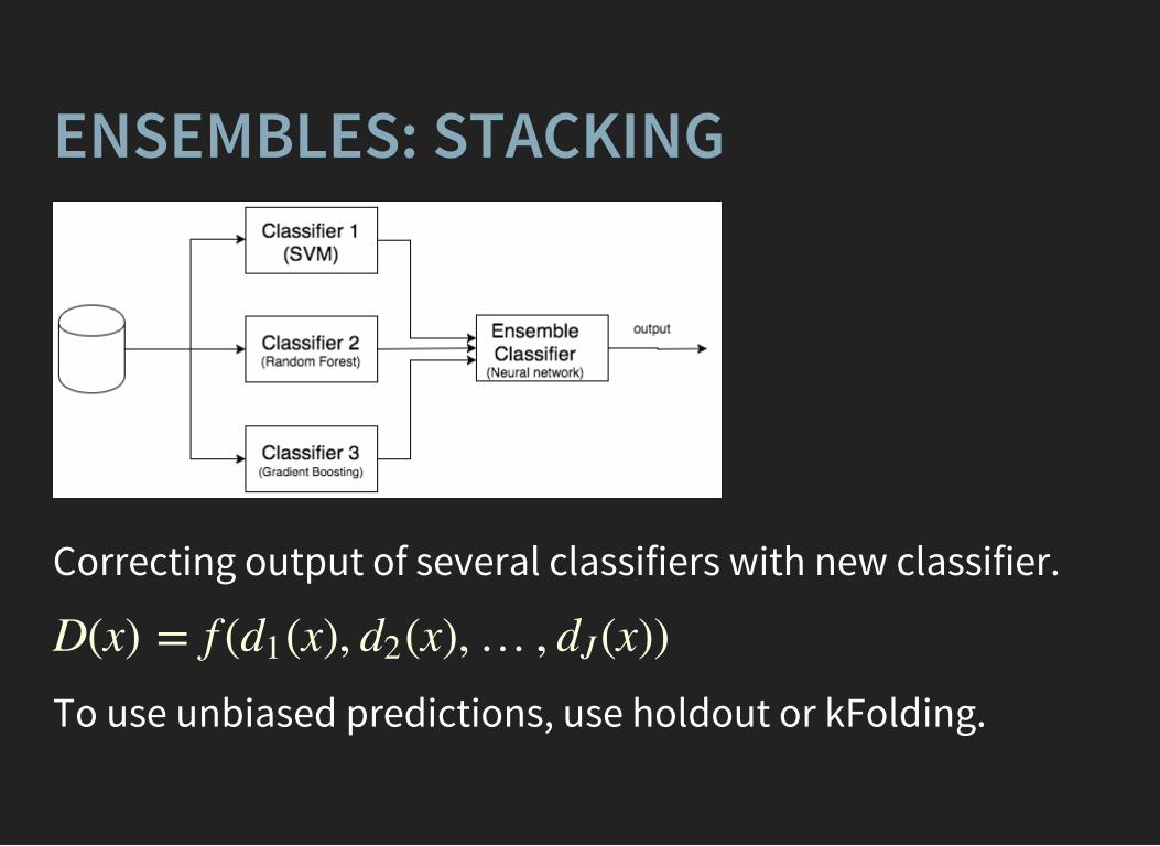
ENSEMBLES: STACKING

Correcting output of several classifiers with new classifier.

D(x) = f ( (x), (x),… , (x))d1 d2 dJ

To use unbiased predictions, use holdout or kFolding.

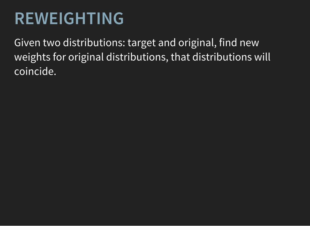
REWEIGHTINGGiven two distributions: target and original, find newweights for original distributions, that distributions willcoincide.

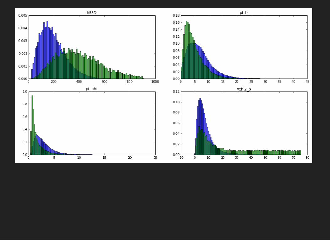
REWEIGHTINGSolution for 1 or 2 variables: reweight using bins (so-called'histogram division').

Typical application: Monte-Carlo reweighting.

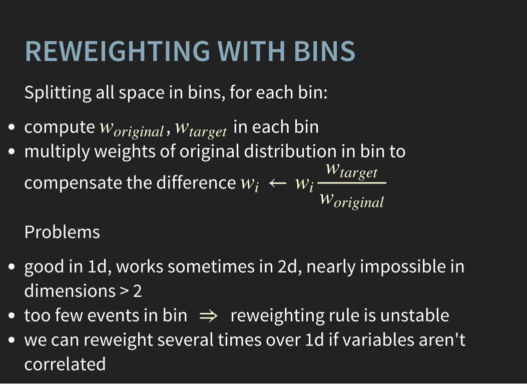
REWEIGHTING WITH BINSSplitting all space in bins, for each bin:

compute , in each binmultiply weights of original distribution in bin to

compensate the difference

woriginal wtarget

←wi wiwtarget

woriginal

Problems

good in 1d, works sometimes in 2d, nearly impossible indimensions > 2too few events in bin reweighting rule is unstablewe can reweight several times over 1d if variables aren'tcorrelated

⇒

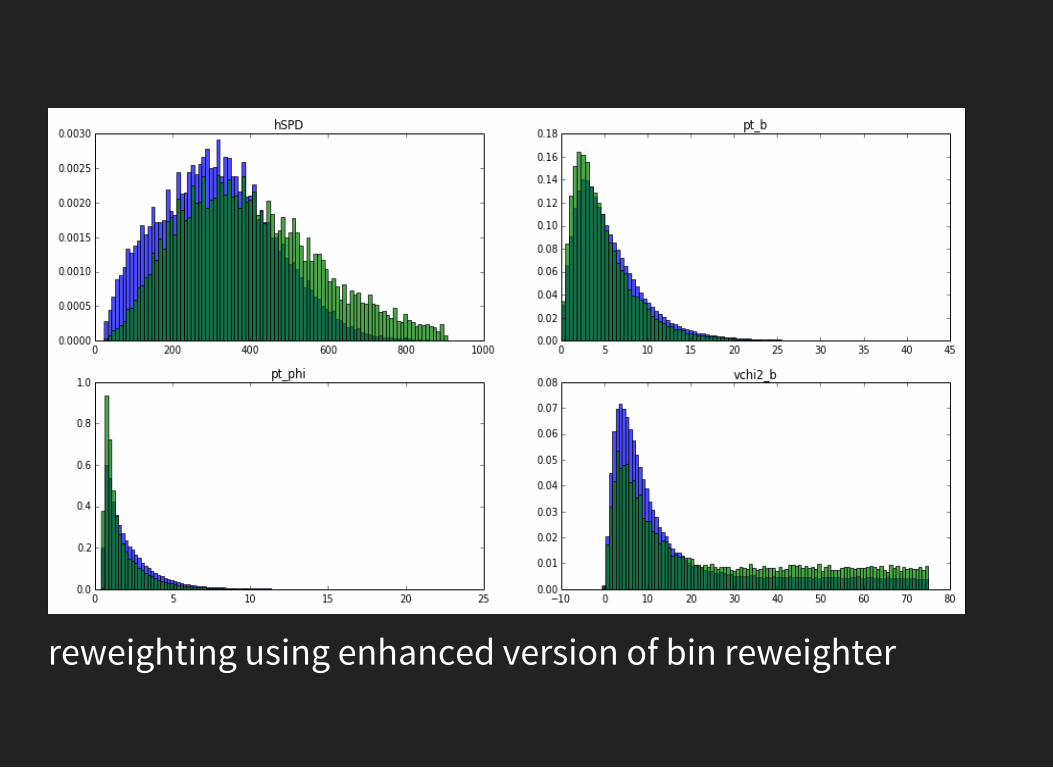
reweighting using enhanced version of bin reweighter

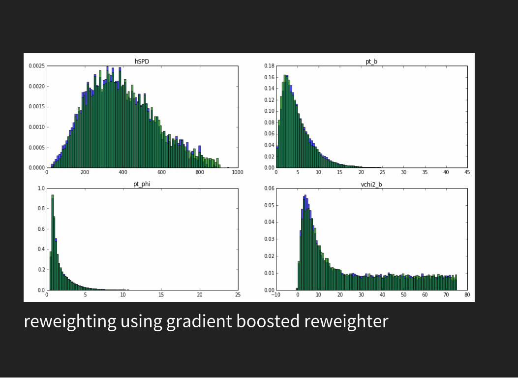
reweighting using gradient boosted reweighter

GRADIENT BOOSTED REWEIGHTERworks well in high dimensionsworks with correlated variablesproduces more stable reweighting rule

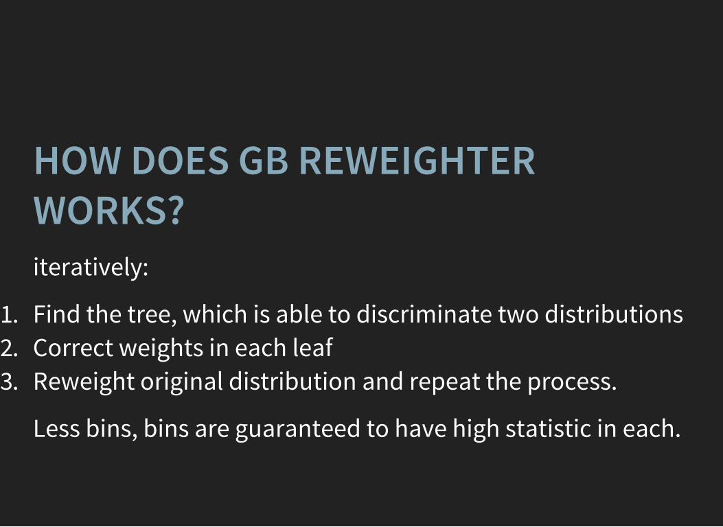
HOW DOES GB REWEIGHTERWORKS?iteratively:

1. Find the tree, which is able to discriminate two distributions2. Correct weights in each leaf3. Reweight original distribution and repeat the process.

Less bins, bins are guaranteed to have high statistic in each.

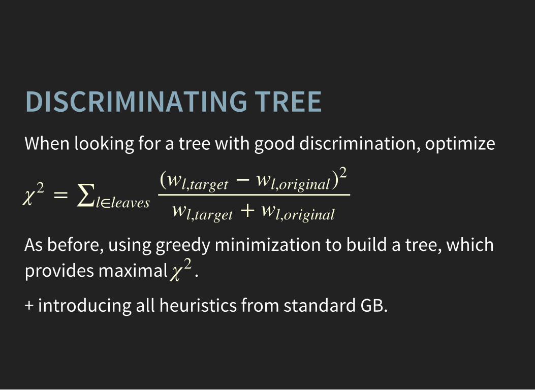
DISCRIMINATING TREEWhen looking for a tree with good discrimination, optimize

=χ2 *l!leaves( +wl,target wl,original)2

+wl,target wl,original

As before, using greedy minimization to build a tree, whichprovides maximal .χ2

+ introducing all heuristics from standard GB.

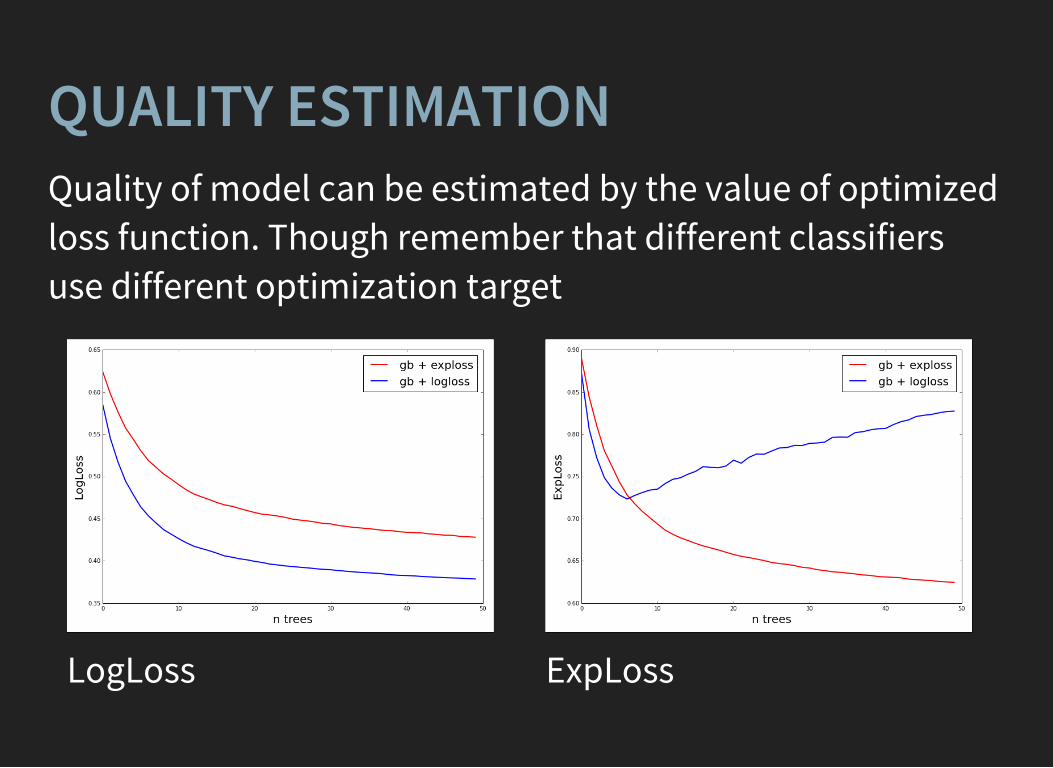
QUALITY ESTIMATIONQuality of model can be estimated by the value of optimizedloss function. Though remember that different classifiersuse different optimization target

LogLoss

ExpLoss

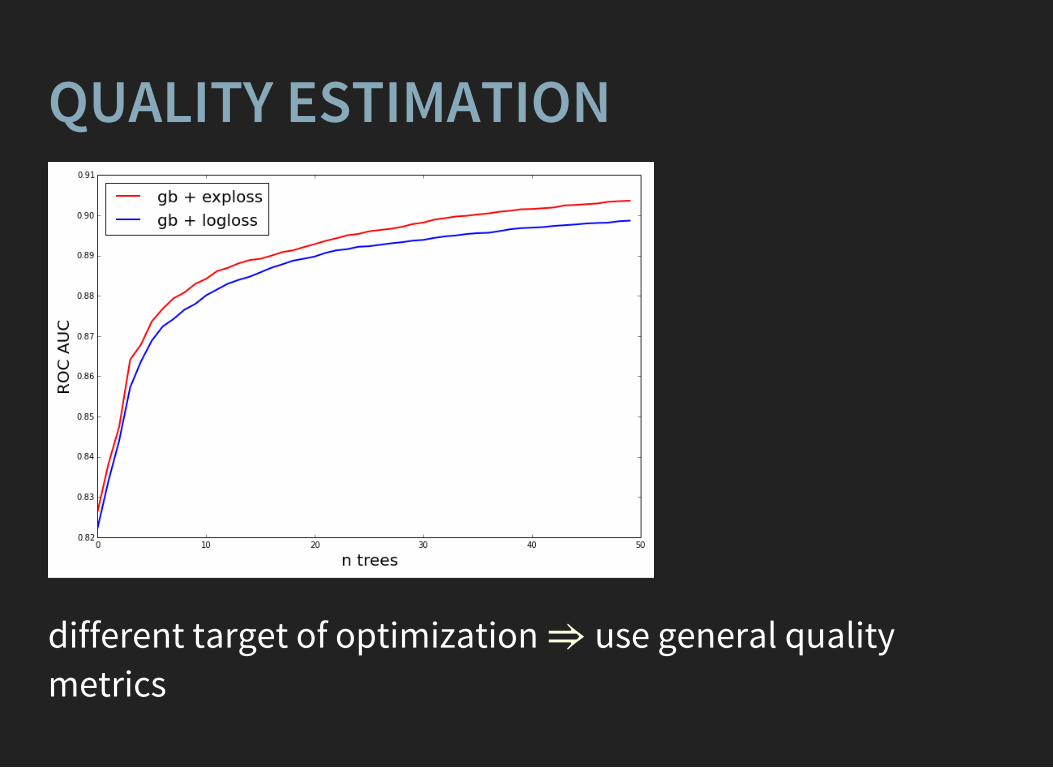
QUALITY ESTIMATION

different target of optimization use general qualitymetrics

⇒

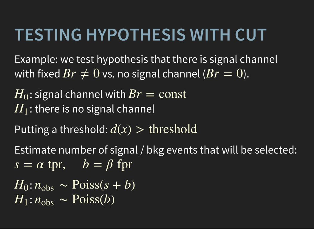
TESTING HYPOTHESIS WITH CUTExample: we test hypothesis that there is signal channelwith fixed vs. no signal channel ( ).Br y 0 Br = 0

: signal channel with : there is no signal channel

H0 Br = constH1

Putting a threshold: d(x) > threshold

Estimate number of signal / bkg events that will be selected:s = α tpr, b = β fpr

: :

H0 U Poiss(s + b)nobsH1 U Poiss(b)nobs

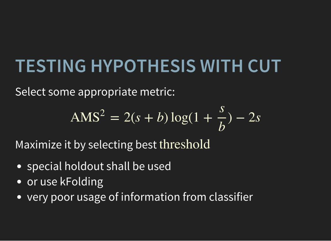
TESTING HYPOTHESIS WITH CUTSelect some appropriate metric:

= 2(s + b) log(1 + ) + 2sAMS2 sb

Maximize it by selecting best

special holdout shall be usedor use kFoldingvery poor usage of information from classifier

threshold

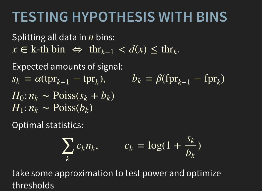
TESTING HYPOTHESIS WITH BINSSplitting all data in bins:

.n

x ! k-th bin ⇔ < d(x) }thrk+1 thrk

Expected amounts of signal: = α( + ), = β( + )sk tprk+1 tprk bk fprk+1 fprk

: :

H0 U Poiss( + )nk sk bkH1 U Poiss( )nk bk

Optimal statistics:

, = log(1 + )∑k

cknk cksk

bk

take some approximation to test power and optimizethresholds

thresholds

FINDING OPTIMAL PARAMETERSsome algorithms have many parametersnot all the parameters are guessedchecking all combinations takes too long

FINDING OPTIMAL PARAMETERSrandomly picking parameters is a partial solutiongiven a target optimal value we can optimize itno gradient with respect to parametersnoisy resultsfunction reconstruction is a problem

Before running grid optimization make sure your metric isstable (i.e. by train/testing on different subsets).

Overfitting by using many attempts is real issue.

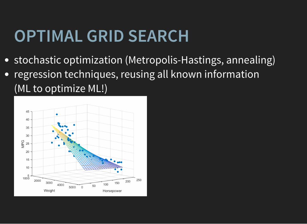
OPTIMAL GRID SEARCHstochastic optimization (Metropolis-Hastings, annealing)regression techniques, reusing all known information (ML to optimize ML!)

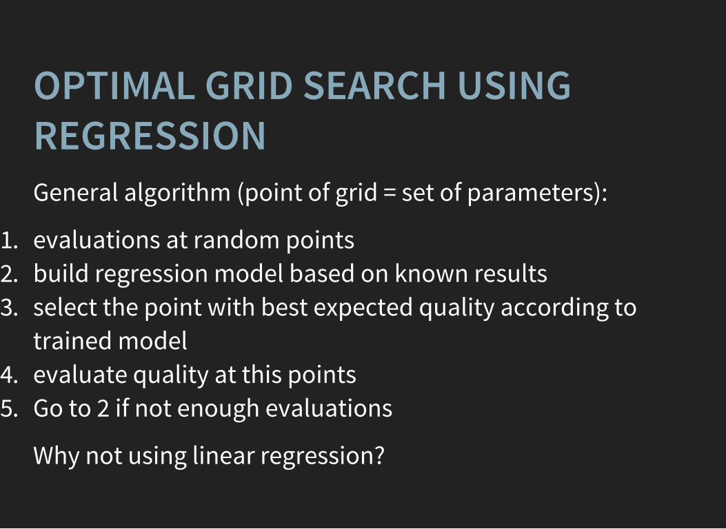
OPTIMAL GRID SEARCH USINGREGRESSIONGeneral algorithm (point of grid = set of parameters):

1. evaluations at random points2. build regression model based on known results3. select the point with best expected quality according to

trained model4. evaluate quality at this points5. Go to 2 if not enough evaluations

Why not using linear regression?

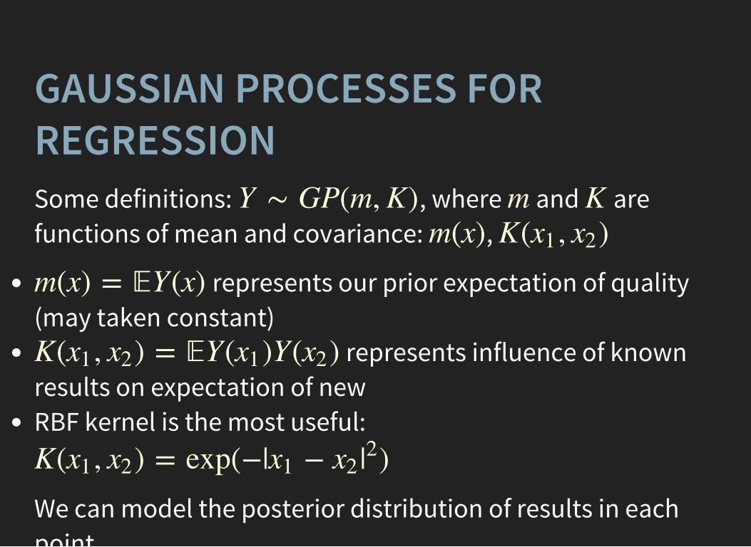
GAUSSIAN PROCESSES FORREGRESSIONSome definitions: , where and arefunctions of mean and covariance: ,

Y U GP(m, K) m Km(x) K( , )x1 x2

represents our prior expectation of quality(may taken constant)

represents influence of knownresults on expectation of newRBF kernel is the most useful:

m(x) = �Y(x)

K( , ) = �Y( )Y( )x1 x2 x1 x2

K( , ) = exp(+| + )x1 x2 x1 x2 |2

We can model the posterior distribution of results in eachpoint.

point.

Gaussian Process Demo on Mathematica

Also see: .http://www.tmpl.fi/gp/

MINUTES BREAKx

PREDICTION SPEEDCuts vs classifier

cuts are interpretablecuts are applied really fastML classifiers are applied much slower

SPEED UP WAYSMethod-specific

Logistic regression: sparsityNeural networks: removing neuronsGBDT: pruning by selecting best trees

Staging of classifiers (a-la triggers)

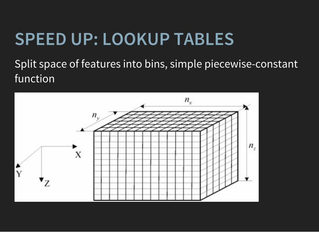
SPEED UP: LOOKUP TABLESSplit space of features into bins, simple piecewise-constantfunction

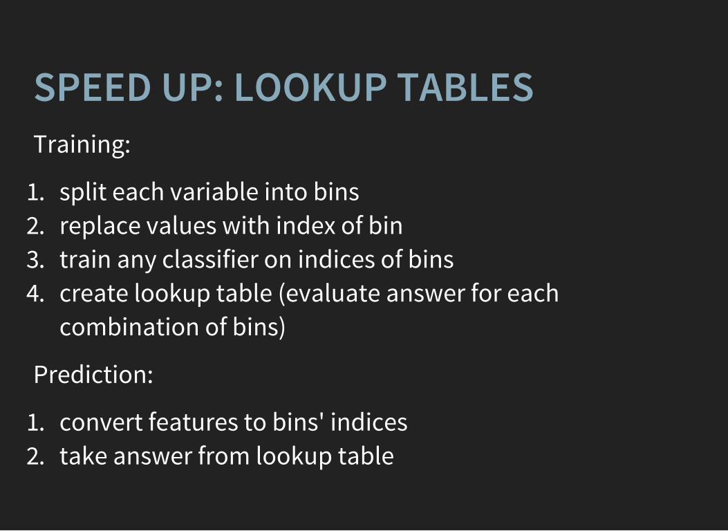
SPEED UP: LOOKUP TABLESTraining:

1. split each variable into bins2. replace values with index of bin3. train any classifier on indices of bins4. create lookup table (evaluate answer for each

combination of bins)

Prediction:

1. convert features to bins' indices2. take answer from lookup table

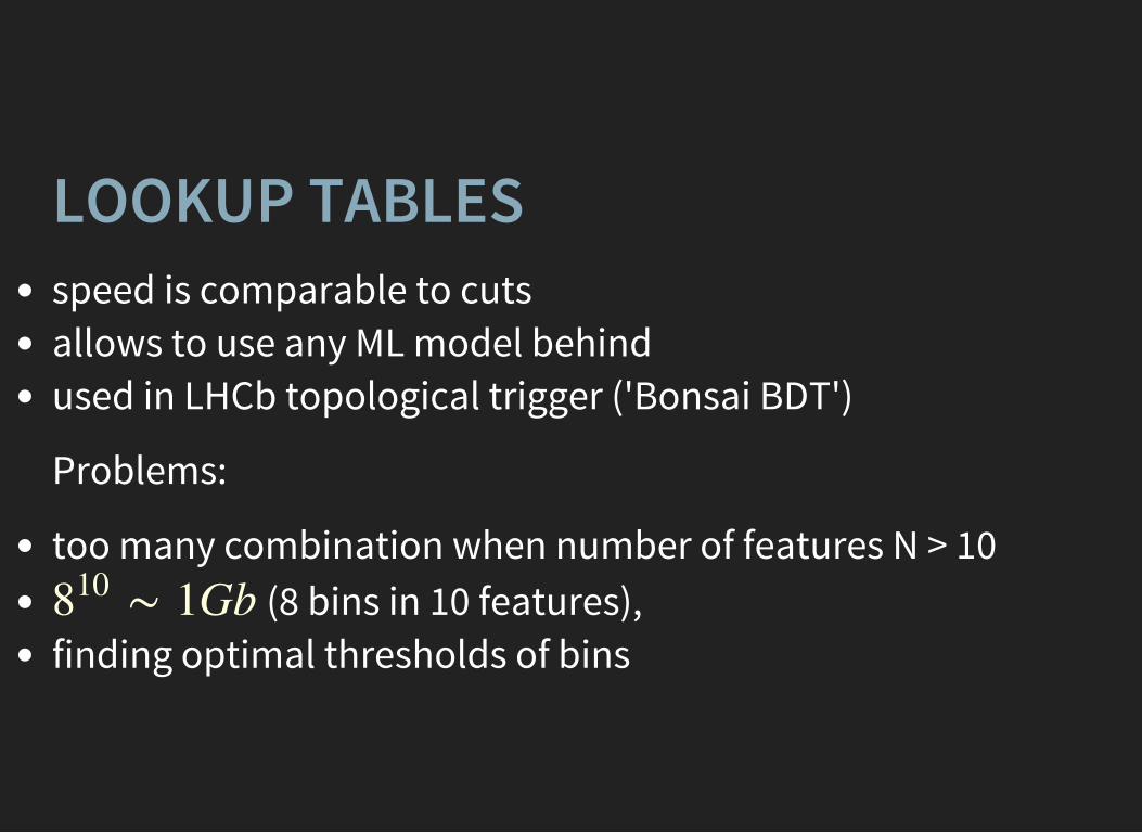
LOOKUP TABLESspeed is comparable to cutsallows to use any ML model behindused in LHCb topological trigger ('Bonsai BDT')

Problems:

too many combination when number of features N > 10 (8 bins in 10 features),

finding optimal thresholds of binsU 1Gb810

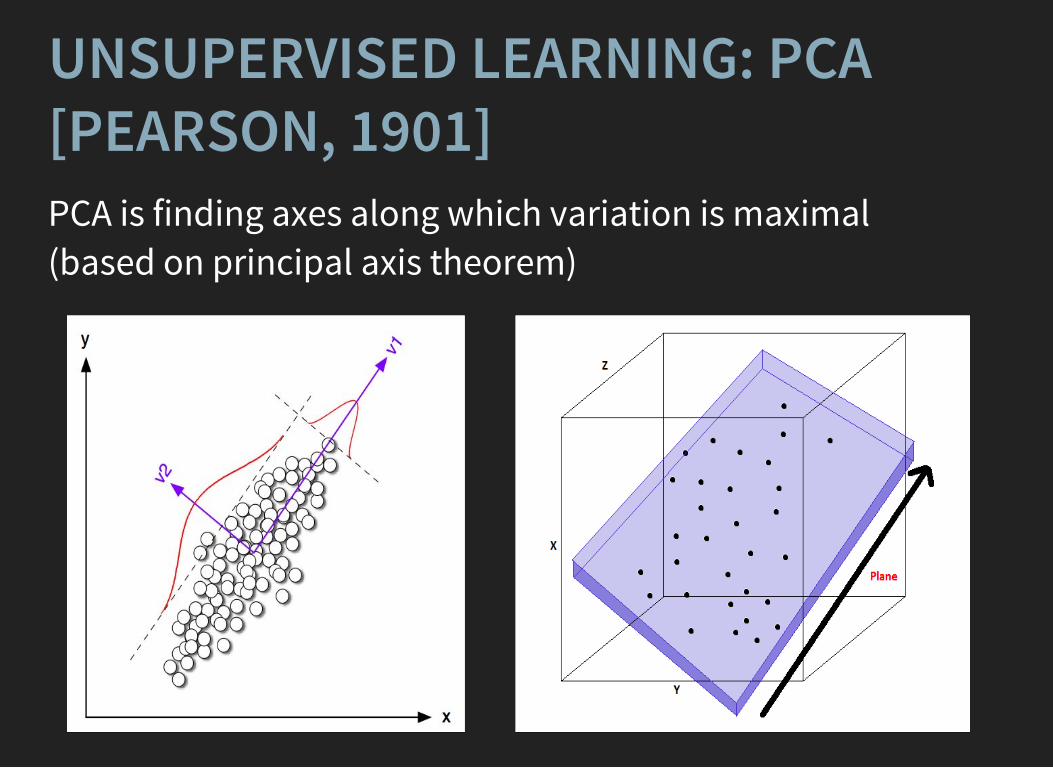
UNSUPERVISED LEARNING: PCA[PEARSON, 1901]PCA is finding axes along which variation is maximal (based on principal axis theorem)

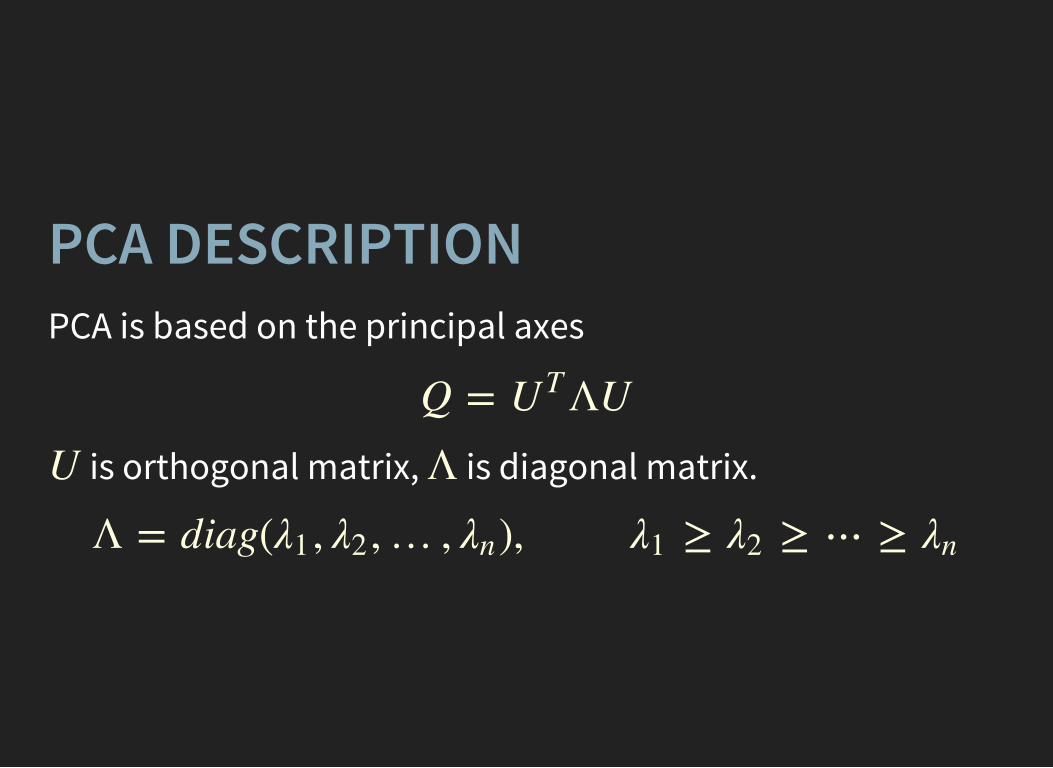
PCA DESCRIPTIONPCA is based on the principal axes

is orthogonal matrix, is diagonal matrix.

Q = ΛUUT

U ΛΛ = diag( , ,… , ), ~ ~ ⋯ ~λ1 λ2 λn λ1 λ2 λn

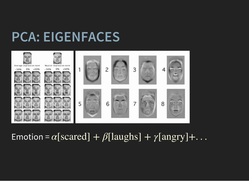
PCA: EIGENFACES

Emotion = α[scared] + β[laughs] + γ[angry]+. . .

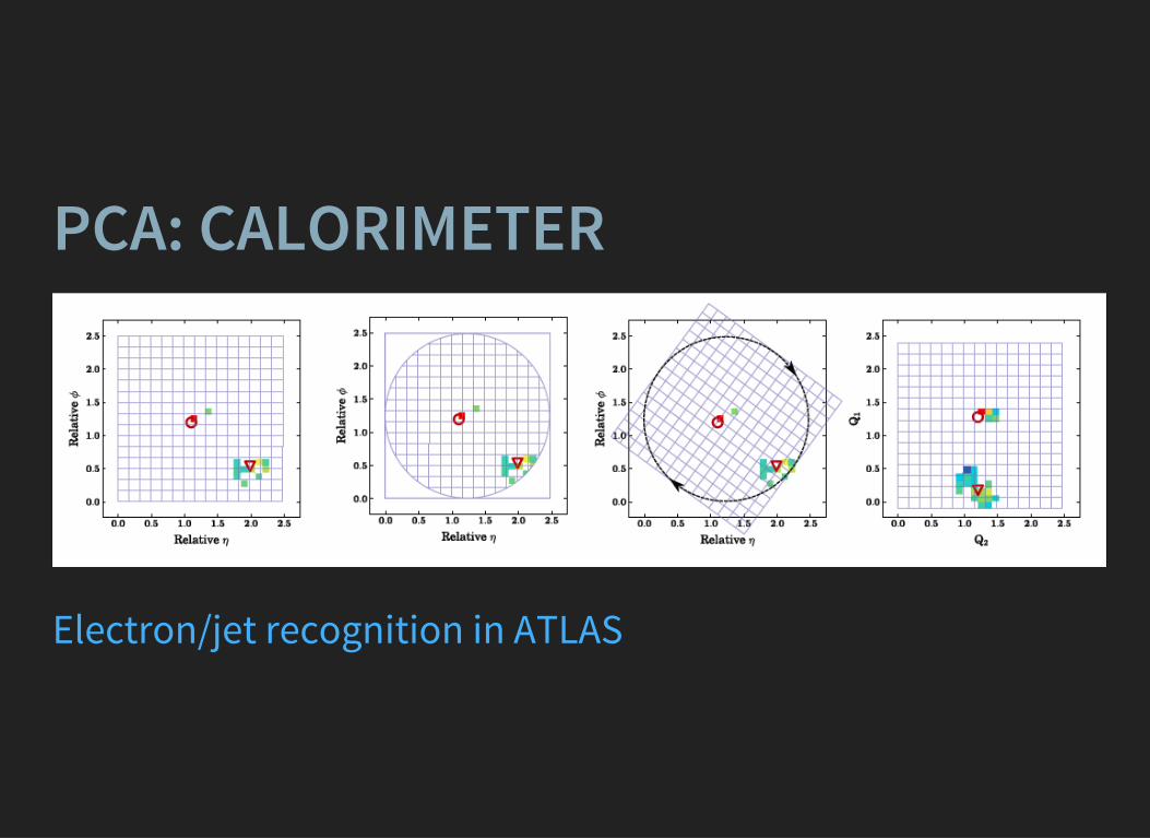
PCA: CALORIMETER

Electron/jet recognition in ATLAS

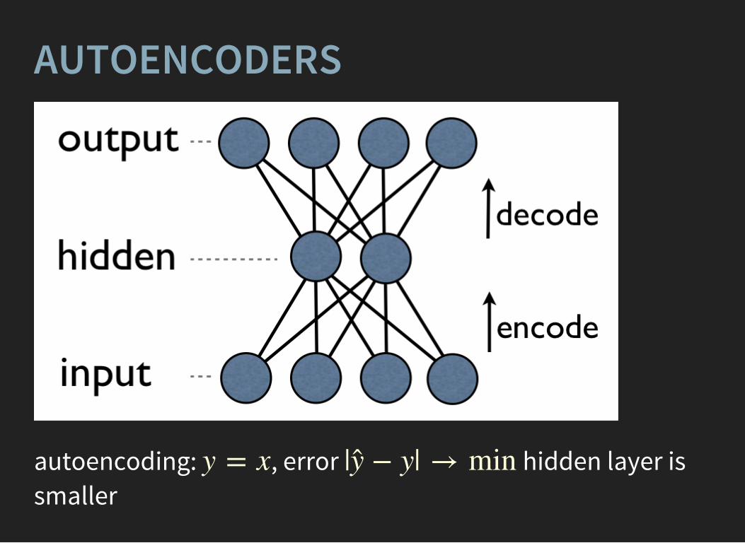
AUTOENCODERS

autoencoding: , error hidden layer issmaller

y = x | + y| → miny ̂

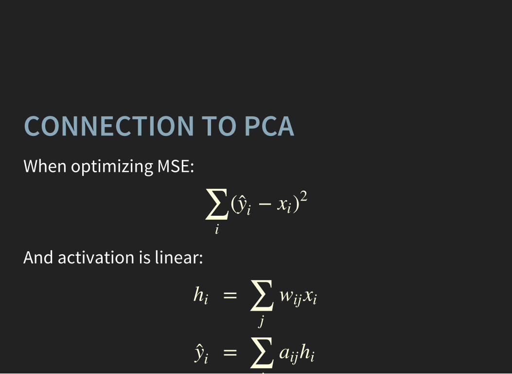
CONNECTION TO PCAWhen optimizing MSE:

( +∑i

y ̂ i xi)2

And activation is linear:

hi

y ̂ i

=

=

∑j

wijxi

∑j

aijhi

j

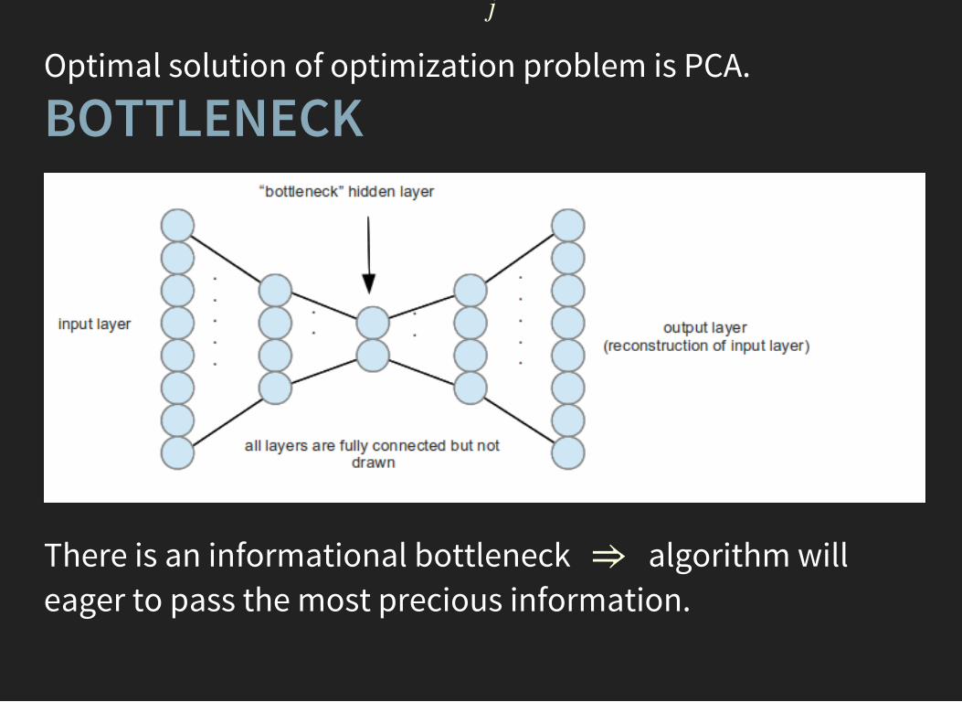
Optimal solution of optimization problem is PCA.

BOTTLENECK

There is an informational bottleneck algorithm willeager to pass the most precious information.

⇒

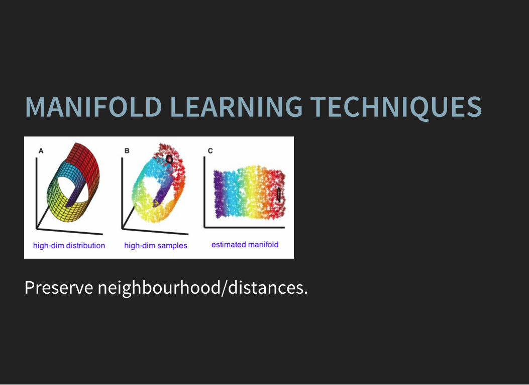
MANIFOLD LEARNING TECHNIQUES

Preserve neighbourhood/distances.

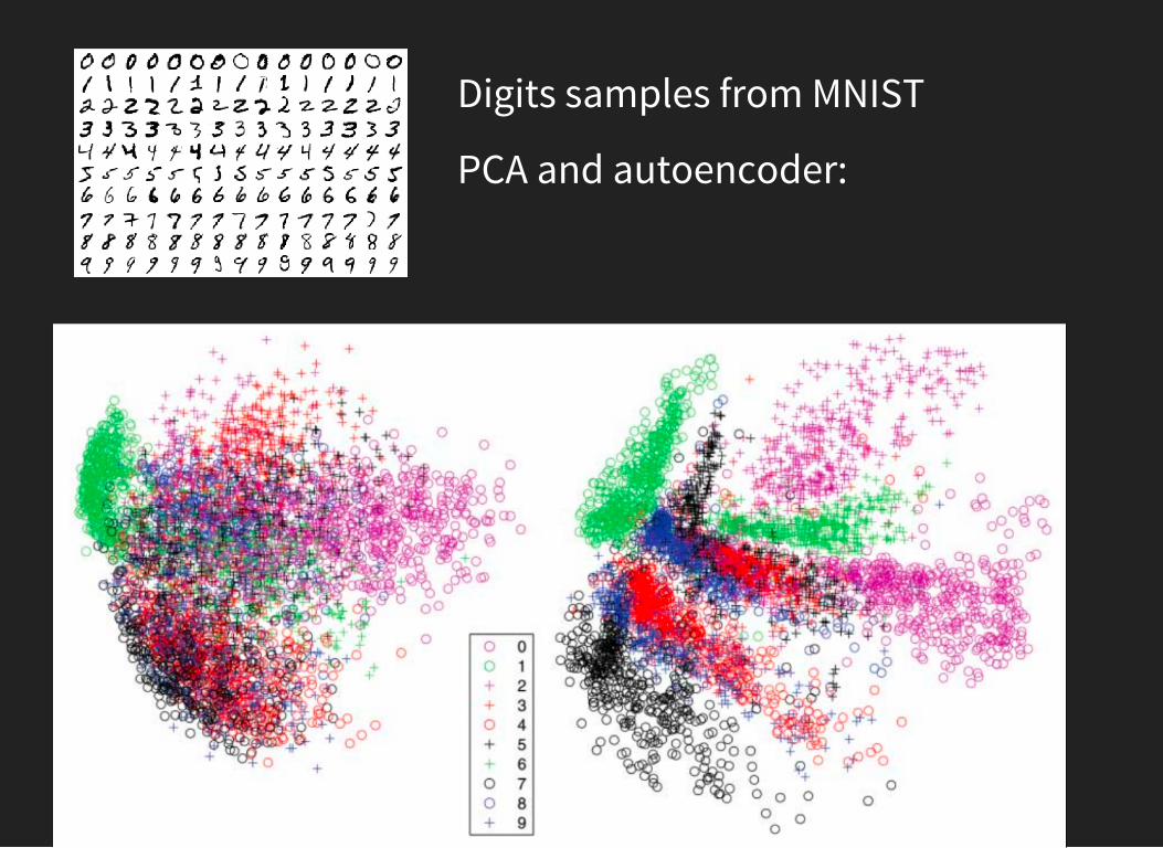
Digits samples from MNIST

PCA and autoencoder:

PART-OF-SPEECH TAGGING

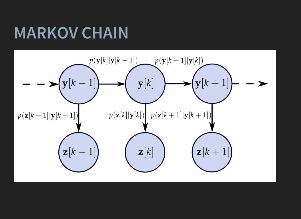
MARKOV CHAIN

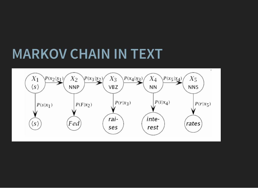
MARKOV CHAIN IN TEXT

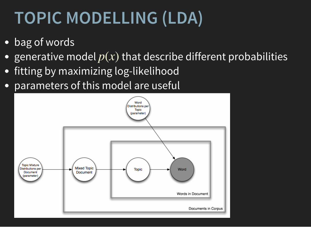
TOPIC MODELLING (LDA)bag of wordsgenerative model that describe different probabilitiesfitting by maximizing log-likelihoodparameters of this model are useful

p(x)

COLLABORATIVE RESEARCHproblem: different environmentsproblem: data ping-pongsolution: dedicated machine (server) for a teamrestart the research = run script or notebook!ping www.bbc.co.uk

REPRODUCIBLE RESEARCHreadable codecode + description + plots togetherkeep versions + reviews

Solution: IPython notebook + github

Example notebook

EVEN MORE REPRODUCIBILITY?Analysis preservation: VM with all needed stuff.Docker

BIRD'S EYE VIEW TO ML:ClassificationRegressionRankingDimensionality reduction

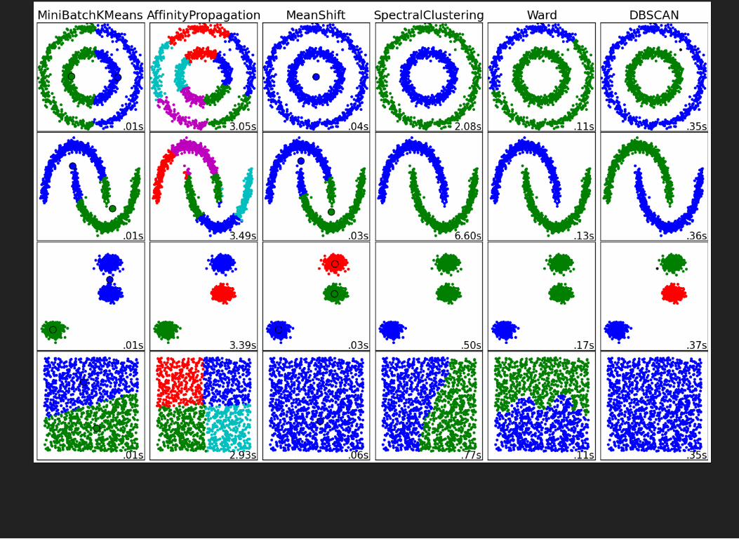
CLUSTERING

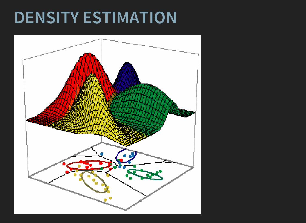
DENSITY ESTIMATION

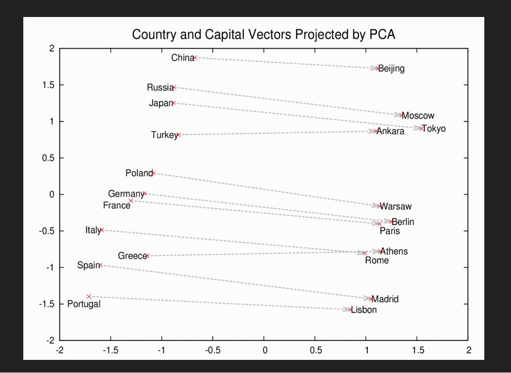
REPRESENTATION LEARNINGWord2vec finds representations of words.

THE END