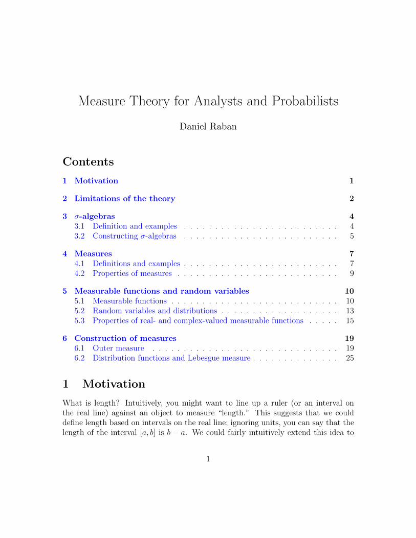
Measure Theory for Analysts and Probabilists

Daniel Raban

Contents

1 Motivation 1

2 Limitations of the theory 2

3 σ-algebras 43.1 Definition and examples . . . . . . . . . . . . . . . . . . . . . . . . . 43.2 Constructing σ-algebras . . . . . . . . . . . . . . . . . . . . . . . . . 5

4 Measures 74.1 Definitions and examples . . . . . . . . . . . . . . . . . . . . . . . . . 74.2 Properties of measures . . . . . . . . . . . . . . . . . . . . . . . . . . 9

5 Measurable functions and random variables 105.1 Measurable functions . . . . . . . . . . . . . . . . . . . . . . . . . . . 105.2 Random variables and distributions . . . . . . . . . . . . . . . . . . . 135.3 Properties of real- and complex-valued measurable functions . . . . . 15

6 Construction of measures 196.1 Outer measure . . . . . . . . . . . . . . . . . . . . . . . . . . . . . . 196.2 Distribution functions and Lebesgue measure . . . . . . . . . . . . . . 25

1 Motivation

What is length? Intuitively, you might want to line up a ruler (or an interval onthe real line) against an object to measure “length.” This suggests that we coulddefine length based on intervals on the real line; ignoring units, you can say that thelength of the interval [a, b] is b − a. We could fairly intuitively extend this idea to

1

finite unions and intersections of intervals; just add the lengths of disjoint intervals.But what about other subsets of R? Can we extend the idea of length to Z, Q, orcomplicated fractal-like subsets of R?

What about area? This might seem even harder to define. More generally, it isa common desire to want to assign a number or a value to a set. We want to assignarea or volume to subsets of R2 or R3. Maybe we have a distribution of mass in R3,and we want to be able to see how much mass is in any kind of set, even a fractal-likeset (maybe this brings to mind an idea of integration). Or maybe we have a set ofoutcomes of some situation, and we want to define probabilities of subsets of theseoutcomes.

At the most basic level, measure theory is the theory of assigning a number, viaa “measure,” to subsets of some given set. Measure theory is the basic language ofmany disciplines, including analysis and probability. Measure theory also leads to amore powerful theory of integration than Riemann integration, and formalizes manyintuitions about calculus.

2 Limitations of the theory

Before actually constructing measures, we must first devote some discussion to afundamental limitation of the theory. In particular, it is not always possible tomeasure all subsets of a given set. We illustrate this with an example:

Example 2.1 (Vitali set). Let’s assume we can measure all subsets of R, with somefunction µ : P(R)→ [0,∞] that takes subsets of R and assigns them a “length.” Inparticular, let’s assume that µ has the following properties:

1. µ([0, 1)) = 1.

2. If sets Ai are mutually disjoint, µ(⋃iAi) =

∑i µ(Ai).

3. For all x ∈ R, µ(A) = µ(A + x), where A + x := a + x : a ∈ A (invarianceunder translation).

Define an equivalence relation on [0, 1) as follows: x ∼ y ⇐⇒ x = y + q forsome q ∈ Q. This partitions [0, 1) into equivalence classes of numbers that are closedunder addition by rational numbers. Let N be a set containing exactly one member

2

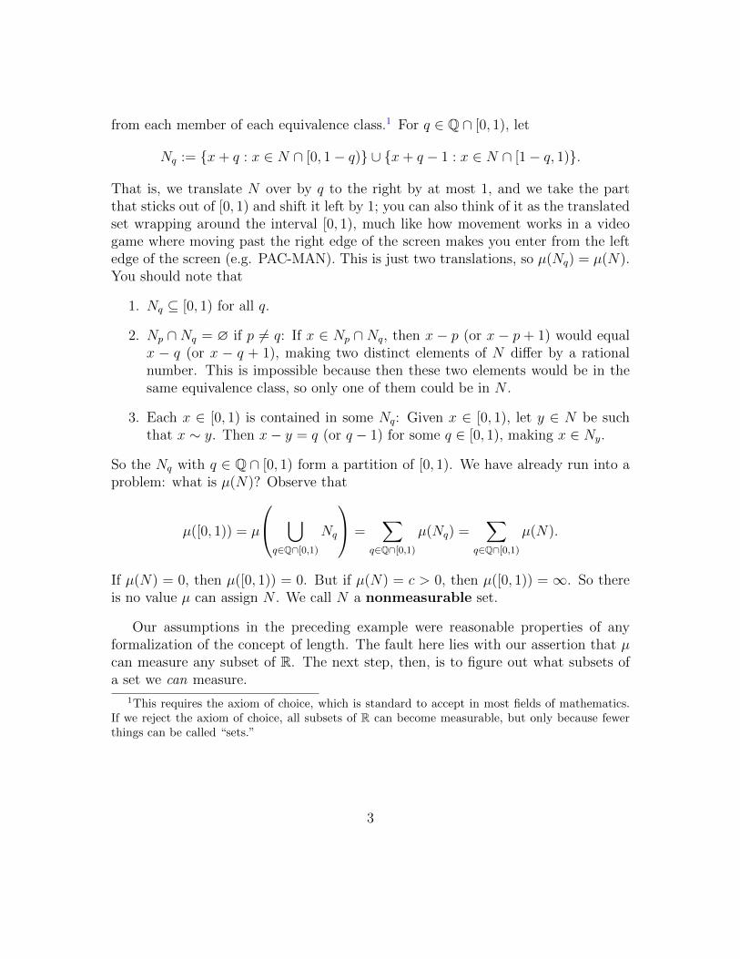
from each member of each equivalence class.1 For q ∈ Q ∩ [0, 1), let

Nq := x+ q : x ∈ N ∩ [0, 1− q) ∪ x+ q − 1 : x ∈ N ∩ [1− q, 1).

That is, we translate N over by q to the right by at most 1, and we take the partthat sticks out of [0, 1) and shift it left by 1; you can also think of it as the translatedset wrapping around the interval [0, 1), much like how movement works in a videogame where moving past the right edge of the screen makes you enter from the leftedge of the screen (e.g. PAC-MAN). This is just two translations, so µ(Nq) = µ(N).You should note that

1. Nq ⊆ [0, 1) for all q.

2. Np ∩ Nq = ∅ if p 6= q: If x ∈ Np ∩ Nq, then x − p (or x − p + 1) would equalx − q (or x − q + 1), making two distinct elements of N differ by a rationalnumber. This is impossible because then these two elements would be in thesame equivalence class, so only one of them could be in N .

3. Each x ∈ [0, 1) is contained in some Nq: Given x ∈ [0, 1), let y ∈ N be suchthat x ∼ y. Then x− y = q (or q − 1) for some q ∈ [0, 1), making x ∈ Ny.

So the Nq with q ∈ Q ∩ [0, 1) form a partition of [0, 1). We have already run into aproblem: what is µ(N)? Observe that

µ([0, 1)) = µ

⋃q∈Q∩[0,1)

Nq

=∑

q∈Q∩[0,1)

µ(Nq) =∑

q∈Q∩[0,1)

µ(N).

If µ(N) = 0, then µ([0, 1)) = 0. But if µ(N) = c > 0, then µ([0, 1)) = ∞. So thereis no value µ can assign N . We call N a nonmeasurable set.

Our assumptions in the preceding example were reasonable properties of anyformalization of the concept of length. The fault here lies with our assertion that µcan measure any subset of R. The next step, then, is to figure out what subsets ofa set we can measure.

1This requires the axiom of choice, which is standard to accept in most fields of mathematics.If we reject the axiom of choice, all subsets of R can become measurable, but only because fewerthings can be called “sets.”

3

3 σ-algebras

3.1 Definition and examples

Definition 3.1. Let let X be any set. A σ-algebra (or σ-field)2 F ⊆ P(X) is acollection of subsets of X such that

1. F 6= ∅.

2. If E ∈ F , then Ec ∈ F .

3. If E1, E2, . . . ∈ F , then⋃∞i=1 Ei ∈ F .

In other words, a σ-algebra is a nonempty collection that is closed under set com-plements and countable unions. The definition also implies closure under countableintersections because

⋂∞n=1 En = (

⋃∞n=1E

cn)c.

Example 3.1. Let X be any set. Then P(X) is a σ-algebra.

Remark 3.1. You might wonder what the whole point of defining σ-algebras was,since P(X) is a σ-algebra. Indeed, using P(R) as a σ-algebra for our “length”measure would be no different from if we had not introduced σ-algebras at all. Thekey point to realize here is that some measures with desired properties (such astranslation invariance) will be defined on smaller σ-algebras, while other measuresmay be defined on larger σ-algebras, even P(X).

Example 3.2. Let X be any set. The collection F = ∅, X is a σ-algebra.

In fact, this is in some sense the minimal σ-algebra on a set.

Proposition 3.1. Let F ⊆P(X) be a σ-algebra. Then ∅, X ∈ F .

Proof. The collection F is nonempty, so there exists some E ∈ F . Then Ec ∈ F ,and we get that X = E ∪ Ec ∪ · · · ∈ F . Moreover, ∅ = Xc ∈ F .

So a σ-algebra is also closed under finite unions, since⋃ni=1Ei =

⋃ni=1 Ei ∪ ∅ ∪

∅ ∪ · · · . The same holds for finite intersections. Here is a nontrivial example of aσ-algebra.

Example 3.3. Let X be an uncountable set. Then the collection

F := E ⊆ X : E is countable or Ec is countable

is a σ-algebra.2These are not to be confused with algebras and fields from abstract algebra. In my experience,

analysts use the term σ-algebra, and probabilists use σ-field.

4

3.2 Constructing σ-algebras

How do we construct σ-algebras? Often, it is difficult to just define a set that containswhat we want. Sometimes, it is useful to create σ-algebras from other σ-algebras orfrom other collections of sets, such as a topology.

Proposition 3.2. Let Fα : α ∈ A be a collection of σ-algebras on a set X. ThenF =

⋂α∈AFα is a σ-algebra.

Proof. We check the 3 parts of the definition.

1. Nonemptiness: F 6= ∅ because X ∈ Fα for each α ∈ A.

2. Closure under complements: If E ∈ F , then E ∈ Fα for each α ∈ A. Every Fαis a σ-algebra and is closed under complements, so Ec ∈ Fα for each α ∈ A.Then Ec ∈

⋂α∈AFα = F .

3. Closure under countable unions: If Ei ∈ F for each i ∈ N, then all the Ei ∈ Fαfor each α ∈ A. Every Fα is a σ-algebra and is closed under countable unions,so⋃∞i=1Ei ∈ Fα for each α ∈ A. Then

⋃∞i=1Ei ∈

⋂α∈AFα = F .

We now introduce one of the most common ways to construct a σ-algebra. Thisconstruction closely mirrors other constructions in mathematics, such as closures ofsets in topology and ideals generated by elements in ring theory.

Definition 3.2. Let E be a collection of subsets of a set X. The σ-algebra gen-erated by E , denoted σ(E), is the smallest σ-algebra containing E . That is, σ(E) isthe intersection of all σ-algebras containing E.

Why is this intersection well defined? There is always one σ-algebra containing E ,namely P(X). Now we can introduce possibly the most commonly used σ-algebra.

Example 3.4. Let X be a nonempty set, let A ⊆ X, and let E = A. Thenσ(E) = ∅, A,Ac, X. If you take B ⊆ X and let E ′ = A,B, then σ(E ′) containssets such as A,B,Ac, A∪B,A∩Bc, (A∪B)c, . . . . Constructing the σ-field generatedby a collection of sets creates a large collection of sets to measure.

Example 3.5. Let X be a metric space (or topological space), and let T be thecollection of open subsets of X. Then the Borel σ-algebra is given by BX = σ(T ).This σ-algebra contains open sets, closed sets, and more. We most commonly useBR, which we will sometimes denote by B. When we talk about BRd , we assume theEuclidean metric.3

3We can actually use any metric induced by a norm on Rd, since all norms on a finite-dimensionalR-valued vector space induce equivalent metrics.

5

Example 3.6. What kinds of sets are in B = BR? By definition, B contains allopen intervals and unions of open intervals. Since closed sets are complements ofopen sets, B contains all closed intervals, as well. For any x ∈ R, x ∈ B becausex =

⋂∞n=1[x, x+ 1/n]. From this, we get that all countable subsets of R are in B.

In fact, most subsets of R you would ever care about can be found in B, save forpathological sets we might construct, such as the Vitali set.

Here is an example motivated by probability theory.

Example 3.7. Suppose you are flipping a coin repeatedly.4 Define the set of out-comes Ω = H,T∞ := H,T × H,T × · · · . For each n ≥ 1,

Fn = A× H,T × H,T × · · · : A ⊆ H,Tn.

The collection Fn is a σ-field, and contains the events that can be determined aftern flips of the coin. Note that F1 ⊆ F2 ⊆ · · · . We can define F∞, the σ-field of eventsin the whole random process, as σ(

⋃∞n=1Fn). This is actually larger than

⋃∞n=1Fn,

since all events in⋃∞n=1Fn are only determined by finitely many coin flips, while

events in σ(⋃∞n=1Fn) can be dependent on the results of infinitely many coin flips.

The previous example illustrates a fact about σ-algebras that you should be awareof: a union of σ-algebras need not be a σ-algebra.

We can also create σ-algebras on the Cartesian product of sets in a way that“respects” the σ-algebras on the components.

Definition 3.3. Let Xαα∈A be a collection of sets with corresponding σ-algebrasMαα∈A. The product σ-algebra

⊗α∈AMα is the σ-algebra on

∏α∈AXα given

by ⊗α∈A

Mα = σ(π−1α (Eα) : Eα ∈Mα, α ∈ A),

where πα :∏

α∈AXα → Xα.

This definition is almost identical to the definition of the product topology inpoint-set topology. We leave the relationship between these two as an exercise.

Exercise 3.1. Let X and Y be separable metric spaces. Show that BX×Y = BX⊗BY .

4We assume that you have a lot of free time, so you flip the coin infinitely many times.

6

4 Measures

4.1 Definitions and examples

Now that we have introduced σ-fields, we can define measures.

Definition 4.1. Let X be a measure with a σ-algebra F . A measure is a functionµ : F → [0,∞] that satisfies the following properties:

1. µ(∅) = 0.

2. If sets E1, E2, . . . are mutually disjoint, then µ(⋃∞i=1 Ei) =

∑∞i=1 µ(Ei).

The second condition is called countable additivity; the same property alsoholds for only finitely many sets E1, . . . , En (finite additivity) because you can justlet Ei = ∅ for i > n. Note that µ can take on the value ∞; measures that do notare called finite measures.

Definition 4.2. A measure µ on a set X is called σ-finite if there exist countablymany sets E1, E2, . . . such that

⋃∞i=1 Ei = X, and µ(Ei) <∞ for each i.

Sometimes it is easiest to prove statements for sets with finite measure. If ameasure is σ-finite, we can often extend the proof to the whole space by first breakingit down into countably many finite pieces. It is generally rare to deal with measuresthat are not σ-finite, as they can be unruly.

Example 4.1. Let X be any set, equipped with the σ-algebra F = P(X). Thefunction µ(E) = |E| that returns the size of the set is a measure called countingmeasure. Counting measure is σ-finite iff X is countable.

Example 4.2. Let X be any nonempty set, equipped with the σ-algebra F = P(X).Fix some x ∈ X. The function

µ(E) =

1 x ∈ E0 x /∈ E

is a measure called point mass at x.

Example 4.3. Let X be a countable set equipped with F = P(X), and let µ be ameasure on (X,F). Then for any set E ∈ F , µ(E) =

∑x∈E µ(x).

7

Example 4.4. Let µ be a measure on (X,F), and let E ∈ F . Then the functionµE : F → [0,∞], given by

µE(F ) := µ(E ∩ F ),

is a measure on E.

Definition 4.3. A probability measure P on a set Ω, equipped with a σ-field F ,is a measure with P(Ω) = 1.

Example 4.5. Imagine you flip a fair coin once. The set of outcomes is Ω = H,T,and the σ-field of events is F = P(Ω). Define the function P : F → [0, 1] given by(on “rectangles” of events)

P(E) =

0 E = ∅1/2 E = H or T1 E = Ω.

Later, we will learn how to formally extend such a function to a measure on anyset in F . The function P is a probability measure that gives the probability of eachevent occurring.

If we want to flip our coin n times, the set of outcomes is Ωn = H,Tn, ourσ-algebra is Fn = P(Ωn), and we can construct the probability measure

Pn(E1 × · · · × En) =n∏i=1

P(Ei).

If we flip the coin infinitely many times, the set of outcomes is Ω∞ = H,T∞,our σ-field is σ(

⋃∞n=1Fn), and we can construct the probability measure

P∞(E1 × E2 × · · · ) =∞∏i=1

P(Ei).

Here is some terminology.

Definition 4.4. If X is a set, and F ⊆P(X) is a σ-algebra, then the pair (X,F)is called a measurable space. If µ : F → [0,∞] is a measure, then the triple(X,F , µ) is called a measure space.

In probability theory, measure spaces are denoted by (Ω,F ,P).

8

4.2 Properties of measures

Here are four basic facts about probability measures. The first two properties shouldform your “common sense” intuition about what measures are. The third and fourthproperties are very useful formal properties that allow us to determine the measure ofcomplicated sets; they should also inform your intuition about how measures work.

Proposition 4.1. Let (X,F , µ) be a measure space. Then

1. (Monotonicity) If E ⊆ F , then µ(E) ≤ µ(F ).

2. (Subadditivity) µ(⋃∞n=1En) ≤

∑∞n=1 µ(En).

3. (Continuity from below) If E1 ⊆ E2 ⊆ · · · , then µ(⋃∞n=1 En) = limn→∞ µ(En).

4. (Continuity from above) If E1 ⊇ E2 ⊇ · · · , and µ(En) < ∞ for some n, thenµ(⋂∞n=1En) = limn→∞ µ(En).

Proof. To prove 1, note that

µ(E) ≤ µ(E) + µ(E \ F ) = µ(E ∪ (F \ E)) = µ(F ).

To prove 2, define F1 = E1 and Fn+1 = En+1 \⋃ni=1Ei for each n ∈ N; Fn+1 is

the set of new elements in En+1 that E1, . . . , En did not have. Then Fn ⊆ En foreach n, and the Fn are disjoint. So

µ

(∞⋃n=1

En

)= µ

(∞⋃n=1

Fn

)=∞∑n=1

µ(Fn) ≤∞∑n=1

µ(En),

where we used monotonicity for the last step.To prove 3, observe that if E ⊆ F , µ(E)+µ(E\F ) = µ(F ) implies that µ(F \E) =

µ(F )− µ(E). Then, setting E0 = ∅, we get

µ

(∞⋃n=1

En

)= µ

(∞⋃n=1

(En \ En−1)

)=∞∑n=1

µ(En \ En−1) = limn→∞

n∑i=1

µ(En)− µ(En−1)

= limn→∞

µ(En).

To prove 4, first assume (without loss of generality) that µ(E1) <∞; otherwise,we can throw away the first finitely many Ei to make µ(E1) <∞. Then

µ

(∞⋂n=1

En

)= µ

(E1 \

∞⋃n=2

(En−1 \ En)

)= µ(E1)−

∞∑n=2

µ(En−1 \ En)

9

= limn→∞

µ(E1)−n∑i=1

µ(En−1)− µ(En)

= limn→∞

µ(En).

If µ is a probability measure, property 2 is known as the “union bound.” It saysthat the probability of at least one out of a collection of events occurring is less thanthe sum of the probabilities when the events are considered separately.

Why are the continuity properties important? Suppose we had a measure corre-sponding to “area” in R2. If we wanted to find the area of a set E under a curve (asin integration), we could write E =

⋃∞n=1En, where En is some increasing sequence

of successive approximations to the set E, such as approximations using rectangles.This is the basis for a very powerful theory of measure-theoretic integration.

5 Measurable functions and random variables

5.1 Measurable functions

How do measurable spaces interact with each other?

Definition 5.1. Let (X,M) and (Y,N ) be measurable spaces. A measurablefunction f : X → Y is a function such that for all E ∈ N , f−1(E) ∈M.

The idea here is that if we “pull back” measurable subsets of Y to X via f ,they should still be measurable. Here is in some sense the most basic example of ameasurable function.

Example 5.1. Let A be a measurable subset of X. Then the indicator function5

of A,

1A(x) =

1 x ∈ A0 x /∈ A,

is a measurable function from X to (R,B). Indicator functions are extremely impor-tant in both analysis and probability, and they often are the simplest examples ofcomplicated ideas.6

This should look a lot like the topological definition of continuity. In fact, wehave the following proposition.

5Some people call this a “characteristic function.” The term “characteristic function” has mul-tiple meanings elsewhere, but the term “indicator function” does not.

6Be nice to them, and they will help you in return.

10

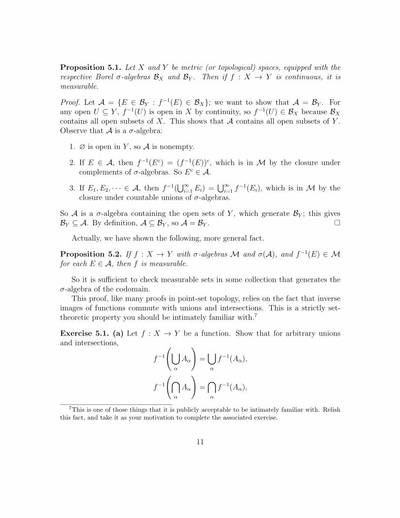
Proposition 5.1. Let X and Y be metric (or topological) spaces, equipped with therespective Borel σ-algebras BX and BY . Then if f : X → Y is continuous, it ismeasurable.

Proof. Let A = E ∈ BY : f−1(E) ∈ BX; we want to show that A = BY . Forany open U ⊆ Y , f−1(U) is open in X by continuity, so f−1(U) ∈ BX because BXcontains all open subsets of X. This shows that A contains all open subsets of Y .Observe that A is a σ-algebra:

1. ∅ is open in Y , so A is nonempty.

2. If E ∈ A, then f−1(Ec) = (f−1(E))c, which is in M by the closure undercomplements of σ-algebras. So Ec ∈ A.

3. If E1, E2, · · · ∈ A, then f−1(⋃∞i=1Ei) =

⋃∞i=1 f

−1(Ei), which is in M by theclosure under countable unions of σ-algebras.

So A is a σ-algebra containing the open sets of Y , which generate BY ; this givesBY ⊆ A. By definition, A ⊆ BY , so A = BY .

Actually, we have shown the following, more general fact.

Proposition 5.2. If f : X → Y with σ-algebras M and σ(A), and f−1(E) ∈ Mfor each E ∈ A, then f is measurable.

So it is sufficient to check measurable sets in some collection that generates theσ-algebra of the codomain.

This proof, like many proofs in point-set topology, relies on the fact that inverseimages of functions commute with unions and intersections. This is a strictly set-theoretic property you should be intimately familiar with.7

Exercise 5.1. (a) Let f : X → Y be a function. Show that for arbitrary unionsand intersections,

f−1

(⋃α

Aα

)=⋃α

f−1(Aα),

f−1

(⋂α

Aα

)=⋂α

f−1(Aα),

7This is one of those things that it is publicly acceptable to be intimately familiar with. Relishthis fact, and take it as your motivation to complete the associated exercise.

11

f−1(Ac) = (f−1(A))c.

(b) Show that

f

(⋃α

Aα

)=⋃α

f(Aα),

and find a counterexample to show that this property does not hold for intersections.

While the previous exercise provides a motivation for the definition of measurablefunctions regarding formal manipulations, the following constructions provide muchmore satisfying motivation.

Example 5.2. Let (X,M, µ) be a measure space, let (Y,N ) be a measurable space,and let f : X → Y be a measurable function. We can define the push-forwardmeasure ν on Y by setting ν(E) = µ(f−1(E)). Check yourself that this is indeed ameasure.

Example 5.3. Here is another way to construct σ-algebras. Given a set X, ameasurable space (Y,N ), and a function f : X → Y , we can construct the pull-back σ-algebra f−1(N ) on X (or the σ-algebra generated by f) as

f−1(N ) = f−1(E) ⊆ X : E ∈ N.

This σ-algebra is also sometimes denoted σ(f). The σ-algebra generated by f is thesmallest σ-algebra on X for which the function f is measurable.

If ν is a measure on Y , we can construct a pull-back measure µ on X by settingµ(f−1(E)) = ν(E). Check yourself that this is indeed a measure. Note, however,that f cannot define a pull-back measure on any σ-algebra on X; this only works forσ-algebras that are smaller than f−1(N ).

Remark 5.1. In general, a composition of measurable functions need not be mea-surable. More explicitly, if f : (X,M) → (Y,N ), and g : (Y,A) → (Z, C), whereN and A are two different σ-algebras on Y , then g f : (X,M) → (Z, C) maynot be measurable. This is very important to remember, as even with R, there aremultiple useful σ-algebras that are common to consider. However, if N = A, thenthe composition g f is measurable.8 Check this yourself; the proof is the same asthat for preservation of continuity under composition of functions.

8For the reader familiar with the language of category theory, this says that measurable functionsare morphisms in the category of measurable spaces. The important distinction here is that in thiscategory, the morphism carries the information of the σ-algebras of the domain and codomain.

12

5.2 Random variables and distributions

Measurable functions have an alternative, yet very important, interpretation in prob-ability theory.

Definition 5.2. Let (Ω,F ,P) be a probability space. Then a random variable Xis a measurable function with domain Ω.

We view Ω as a space of events with some inherent “randomness,” encapsulatedby the probability measure P.

Example 5.4. Let (Ω,F ,P) be a probability space, and let X : Ω → S be aconstant function (i.e. X(ω) = c for some c ∈ S). Then for any σ-field S on S,X is a measurable function. We call X a constant random variable. We ofteninterpret this situation as “deterministic” or having “no randomness.”

Example 5.5. Let X be a real-valued random variable (we implicitly assume theBorel σ-algebra on R). Since f(x) = x2 is continuous, it is measurable (from (R,B)to (R,B)). So X2 is also a random variable. Similarly, aX + b (for a, b ∈ R), sin(X),eX , etc. are random variables.

Often, random variables are specified by their distributions.

Definition 5.3. Let X be a random variable. The distribution of X is its push-forward measure.

To measure the probability of an event on the codomain of a random variable,the distribution “pushes forward” the value from the measure P. In other words, wehave

µ(A) = P(X−1(A)) = P(ω ∈ Ω : X(ω) ∈ A).

We suppress the ω notation and just write

µ(A) = P(X ∈ A).

Usually, we take (Ω,F ,P) to be a certain canonical “reference” measure space(with a measure we will discuss in depth later). For now, take it for granted thatthere is a space Ω with a sufficiently rich measure P that can generate all distributionson R as push-forward measures of random variables.

Example 5.6. Let µ be a probability measure on (−1, 1,P(−1, 1)) given byµ(−1) = µ(1) = 1/2. Let (Ω,F ,P) be our canonical measure space. If X is a

13

measurable function from Ω to −1,−1 with push-forward measure µ, we call X aRademacher random variable. In particular, we have

P(X = 1) := P(ω ∈ Ω : X(ω) ∈ 1) = µ(1) = 1/2,

P(X = −1) := P(ω ∈ Ω : X(ω) ∈ −1) = µ(−1) = 1/2.

Example 5.7. Let’s construct a Poisson random variable. Let µ be a probabilitymeasure on (N,P(N)) given by

µ(k) = e−λλk

k!,

for some real-valued constant λ > 0. Let (Ω,F ,P) be our canonical measure space,and let X be a measurable function from Ω to N with push-forward measure µ. Inparticular,

P(X = k) = µ(k) = e−λλk

k!,

and the probability of any subset of N can be specified by computing a countablesum of P(X = k) for different k.

One of the amazing aspects of measure theory is that is unifies the ideas of discreteand continuous probability (and even allows for mixing of the two). We have covereda few examples of discrete probability spaces above. Here is an example of a non-discrete case.

Example 5.8. A random variable with uniform distribution on [0, 1] (also de-noted as U [0, 1]) is a random variable X with codomain ([0, 1],B[0,1]) and distributionµ that satisfies

µ([a, b]) = P(X ∈ [a, b]) = b− a.for all 0 ≤ a ≤ b ≤ 1. The existence of such a measure is non-obvious, and we shallprove its existence in the next section.

Example 5.9. Here is a distribution on ([0, 1],B[0,1]) that is not discrete but alsohas no continuous probability density over the real numbers. Let

µ(0) = 1/2, µ([a, b]) =

0 0 < a ≤ b < 1/2

b− a 1/2 ≤ a ≤ b ≤ 1.

That is, µ is the uniform distribution but with all the probability in the interval[0, 1/2) “concentrated” onto the value 0. Taking the existence of the uniform distri-bution for granted (moreso the fact that we can define a measure on ([0, 1],B[0,1]) bydefining its value on all subintervals), such a measure is well-defined.

To say that a random variable X has distribution µ, we write X ∼ µ.

14

5.3 Properties of real- and complex-valued measurable func-tions

In this section, we show that sums, products, and limits of real- and complex-valuedmeasurable functions are measurable. Here, we always assume that the σ-algebra onR or C is BR or BC, respectively. The most important parts of this section are notthe results (which are not surprising) but rather the techniques used in the proofs.

Proposition 5.3. Let f, g : X → R be measurable functions. Then the functionsf + g and fg are measurable.

Proof. By the proposition we proved when we introduced the idea of measurablefunctions, it suffices to show that (f + g)−1((a, b)) is measurable for a, b ∈ R; thisis because every nonempty open set in R can be expressed as a countable union ofopen intervals, so these sets generate B. The key property here is that R is separable(i.e. it contains the countable dense set Q).

We have

(f + g)−1((a,∞)) =⋃q∈Q

x : f(x) > q ∩ x : g(x) > a− q

=⋃q∈Q

f−1((q,∞)) ∩ g−1((a− q,∞)),

(f + g)−1((−∞, b)) =⋃q∈Q

x : f(x) < q ∩ x : g(x) < b− q

=⋃q∈Q

f−1((−∞, q)) ∩ g−1((−∞, b− q)),

which are both measurable as countable unions of finite intersections of measurablesets. So

(f + g)−1((a, b)) = (f + g)−1((a,∞)) ∩ (f + g)−1((−∞, b))is measurable as a finite intersection of measurable sets.

To show that fg is measurable, recall that continuous functions from (R,B)to (R,B) are measurable and that compositions of measurable functions (with σ-algebras that match up) are measurable. In particular, the functions x 7→ x2, x 7→ −xand x 7→ x/2 are measurable. So, noting that

fg =1

2

((f + g)2 − f 2 − g2

),

we see that fg is a composition of such measurable functions and is consequentlymeasurable.

15

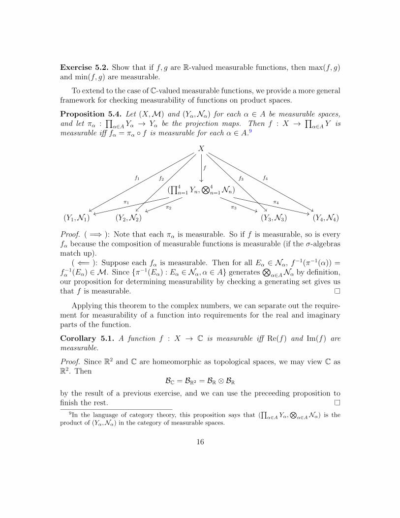
Exercise 5.2. Show that if f, g are R-valued measurable functions, then max(f, g)and min(f, g) are measurable.

To extend to the case of C-valued measurable functions, we provide a more generalframework for checking measurability of functions on product spaces.

Proposition 5.4. Let (X,M) and (Yα,Nα) for each α ∈ A be measurable spaces,and let πα :

∏α∈A Yα → Yα be the projection maps. Then f : X →

∏α∈A Y is

measurable iff fα = πα f is measurable for each α ∈ A.9

X

(∏4

n=1 Yn,⊗4

n=1Nn)

(Y1,N1) (Y2,N2) (Y3,N3) (Y4,N4)

f1 f2 f3 f4

f

π1π2 π3

π4

Proof. ( =⇒ ): Note that each πα is measurable. So if f is measurable, so is everyfα because the composition of measurable functions is measurable (if the σ-algebrasmatch up).

( ⇐= ): Suppose each fα is measurable. Then for all Eα ∈ Nα, f−1(π−1(α)) =f−1α (Eα) ∈M. Since π−1(Eα) : Eα ∈ Nα, α ∈ A generates

⊗α∈ANα by definition,

our proposition for determining measurability by checking a generating set gives usthat f is measurable.

Applying this theorem to the complex numbers, we can separate out the require-ment for measurability of a function into requirements for the real and imaginaryparts of the function.

Corollary 5.1. A function f : X → C is measurable iff Re(f) and Im(f) aremeasurable.

Proof. Since R2 and C are homeomorphic as topological spaces, we may view C asR2. Then

BC = BR2 = BR ⊗ BRby the result of a previous exercise, and we can use the preceeding proposition tofinish the rest.

9In the language of category theory, this proposition says that (∏α∈A Yα,

⊗α∈ANα) is the

product of (Yα,Nα) in the category of measurable spaces.

16

Corollary 5.2. Let f, g : X → C be measurable functions. Then the functions f + gand fg are measurable.

Proof. By the previous corollary, it is sufficient to show that Re(f + g), Im(f + g),Re(fg), and Im(fg) are measurable. Moreover, the same corollary gives us thatRe(f), Im(f), Re(g), and Im(g) are all measurable. We have

Re(f + g) = Re(f) + Re(g), Im(f + g) = Im(f) + Im(g),

Re(fg) = Re(f) Re(g)− Im(f) Im(g), Im(f + g) = Re(f) Im(g) + Im(f) Re(g),

which are measurable as sums and products of measurable real-valued functions.

In probability theory, this gives us an often taken-for-granted result: that sumsand products of random variables are indeed random variables.

What if we have a random process (i.e. a sequence of random variables)? Arelimits of sequences of measurable functions measurable? To talk about limits on thereal line, we must be prepared to have functions take values in R := R ∪ ±∞.Equip R with BR, the σ-algebra generated by E ⊆ R : E ∩ R ∈ BR.10

Proposition 5.5. Let fjj∈N be a sequence of R-valued measurable functions. Thenthe functions

g1(x) := supjfj(x), g2(x) := inf

jfj(x),

g3(x) := lim supj

fj(x), g4(x) := lim infj

fj(x),

are all measurable. Additionally, the set x : limj→∞ fj(x) exists is measurable.

Proof. For g1, it is sufficient to show that g−11 ((a,∞)) is a measurable set because

(a,∞) : a ∈ R generates B; you can check this by checking that countable unionsand intersections of sets in this collection gets you all of the open intervals in R. Wehave that

g−11 ((a,∞)) = x : sup

jfj(x) > a =

⋃j∈N

x : fj(x) > a =⋃j∈N

f−1j ((a,∞)),

which is measurable as a countable union of measurable sets.For measurability of g2, note that

g2(x) = infjfj(x) = − sup

j−fj(x),

10As the notation suggests, this is actually a Borel σ-algebra, induced by a metric on R. Themetric is ρ(x, y) = | arctan(x)− arctan(y)|.

17

which is measurable because the inside is g1 but with the functions −fj.For measurability of g3, let hn(x) := supj≥n fj(x); hn is measurable by the same

reasoning used for g1. Then g3 = infn hn, so g3 is measurable since g2 is measurable.For measurability of g4, note that

g4(x) = lim infj

fj(x) = − lim supj−fj(x),

which is measurable because the inside is g3 but with the functions −fj.Finally, note that

x : limj→∞

fj(x) exists = x : lim supj

fj(x) = lim infj

fj(x)

= x : lim supj

fj(x)− lim infj

fj(x) = 0

= (g3 − g4)−1(0),

which is measurable.

The above proof relied heavily on the countability of the sequence fjj∈N. Ingeneral, the result is not true for uncountable collections of functions.

Corollary 5.3. If fjj∈N is a sequence of R-valued measurable functions, andlimj→∞ fj(x) exists for every x, then f(x) := limj→∞ fj(x) is measurable.

Proof. If limj→∞ fj(x) exists for every x, then f(x) = lim supj fj(x), which is mea-surable by the previous proposition.

Corollary 5.4. If fjj∈N is a sequence of C-valued measurable functions, andlimj→∞ fj(x) exists for every x, then f(x) := limj→∞ fj(x) is measurable.

Proof. If limj→∞ fj(x) exists for every x, then Re(f) = limj→∞Re(fj)(x) and Im(f) =limj→∞ Im(fj)(x) exist for every x and are measurable functions.

We conclude this section with a result that will be important later, when wediscuss distribution functions in additional depth.

Proposition 5.6. If f : R→ R is monotone, it is measurable.

Proof. Without loss of generality, we may assume f is increasing (otherwise considerthe function −f). For each a ∈ R, let xa = supx ∈ R : f(x) < a. We have twocases:

1. If f(xa) ≤ a, then f−1((a,∞)) = x : f(x) > a = (xa,∞).

2. If f(xa) > a, then f−1((a,∞)) = x : f(x) > a = [xa,∞).

So f−1((a,∞)) ∈ B for every a ∈ R. Hence, f is measurable.

18

6 Construction of measures

6.1 Outer measure

Until now, we have been vague about how to construct measures, especially the morecomplicated measures on R. We now develop tools for doing so. These constructionsare sometimes skipped by people who wish to assume the existence of such measuresand treat them as “black boxes.” However, if you go on to do work involving measuretheory, you will invariably run into issues involving measurability, and in such times,knowledge of outer measure will save the day.

Here is some motivation. We have had two main issues so far in constructingmeasures:

1. complicated non-measurable sets,

2. how to actually specify values for a large class of subsets of a measurable space.

Outer measure solves both these issues by “approximating complicated sets usingsimpler sets.” For example, in R2, you can approximate the area under a curve bysuccessively finer coverings of the area by rectangles (as in Riemann integration);you might call this approximation by “outer area.” As an analogy, consider therelationship between the limit and lim sup of a real-valued sequence; the lim supapproximates the limit from above, and we can define the limit as the value of thelim sup under certain conditions (in this case, the lim sup equalling the lim inf).

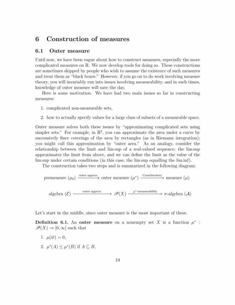
The construction takes two steps and is summarized in the following diagram:

premeasure (µ0) outer measure (µ∗) measure (µ)

algebra (E) P(X) σ-algebra (A)

outer approx. Caratheodory

outer approx. µ∗-measurability

Let’s start in the middle, since outer measure is the most important of these.

Definition 6.1. An outer measure on a nonempty set X is a function µ∗ :P(X)→ [0,∞] such that

1. µ(∅) = 0,

2. µ∗(A) ≤ µ∗(B) if A ⊆ B,

19

3. µ∗(⋃∞i=1 Ai) ≤

∑∞i=1 µ

∗(Ai).

Here is how we construct outer measure using “upper approximation.” Take afunction µ0 which gives us the desired value of a measure on some relatively simpleclass of sets E . Then we can define the outer measure of a set A by taking the bestapproximation of the value of µ0 on coverings of A by simpler sets in E .

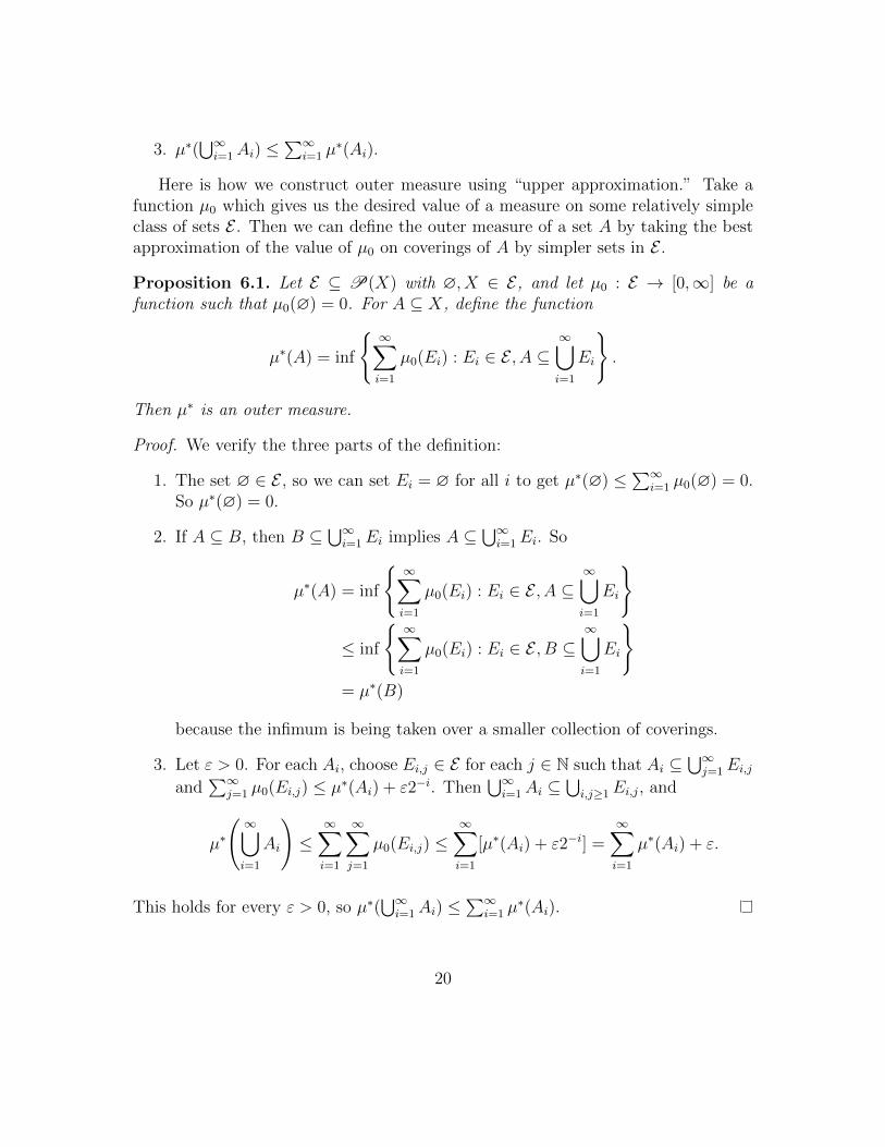
Proposition 6.1. Let E ⊆ P(X) with ∅, X ∈ E, and let µ0 : E → [0,∞] be afunction such that µ0(∅) = 0. For A ⊆ X, define the function

µ∗(A) = inf

∞∑i=1

µ0(Ei) : Ei ∈ E , A ⊆∞⋃i=1

Ei

.

Then µ∗ is an outer measure.

Proof. We verify the three parts of the definition:

1. The set ∅ ∈ E , so we can set Ei = ∅ for all i to get µ∗(∅) ≤∑∞

i=1 µ0(∅) = 0.So µ∗(∅) = 0.

2. If A ⊆ B, then B ⊆⋃∞i=1Ei implies A ⊆

⋃∞i=1Ei. So

µ∗(A) = inf

∞∑i=1

µ0(Ei) : Ei ∈ E , A ⊆∞⋃i=1

Ei

≤ inf

∞∑i=1

µ0(Ei) : Ei ∈ E , B ⊆∞⋃i=1

Ei

= µ∗(B)

because the infimum is being taken over a smaller collection of coverings.

3. Let ε > 0. For each Ai, choose Ei,j ∈ E for each j ∈ N such that Ai ⊆⋃∞j=1Ei,j

and∑∞

j=1 µ0(Ei,j) ≤ µ∗(Ai) + ε2−i. Then⋃∞i=1Ai ⊆

⋃i,j≥1Ei,j, and

µ∗

(∞⋃i=1

Ai

)≤

∞∑i=1

∞∑j=1

µ0(Ei,j) ≤∞∑i=1

[µ∗(Ai) + ε2−i] =∞∑i=1

µ∗(Ai) + ε.

This holds for every ε > 0, so µ∗(⋃∞i=1 Ai) ≤

∑∞i=1 µ

∗(Ai).

20

The verification of the last part of the definition uses a very valuable11 tech-nique: if you wanst to establish inequalities (or equalities) involving an infimum orsupremum, consider an element that almost achieves the infimum (or supremum)but misses it by at most ε. If you’re wondering why an inequality holds (and arestruggling to prove it), sometimes the ε comes in and solves everything like magic. Incases like this, taking a step back and viewing the problem from a a vaguer viewpointof “things approximating other things” should provide you with the intuition youwere missing.

What kind of function is µ0? Defining an outer measure out of any function maylead to issues when we try to make the outer measure into a measure. The followingexample provides some intuition for what nice properties we need.

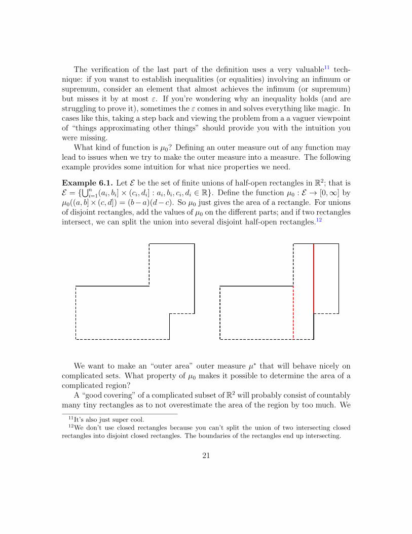
Example 6.1. Let E be the set of finite unions of half-open rectangles in R2; that isE =

⋃ni=1(ai, bi]× (ci, di] : ai, bi, ci, di ∈ R. Define the function µ0 : E → [0,∞] by

µ0((a, b]× (c, d]) = (b−a)(d− c). So µ0 just gives the area of a rectangle. For unionsof disjoint rectangles, add the values of µ0 on the different parts; and if two rectanglesintersect, we can split the union into several disjoint half-open rectangles.12

We want to make an “outer area” outer measure µ∗ that will behave nicely oncomplicated sets. What property of µ0 makes it possible to determine the area of acomplicated region?

A “good covering” of a complicated subset of R2 will probably consist of countablymany tiny rectangles as to not overestimate the area of the region by too much. We

11It’s also just super cool.12We don’t use closed rectangles because you can’t split the union of two intersecting closed

rectangles into disjoint closed rectangles. The boundaries of the rectangles end up intersecting.

21

have built in countable additivity into the function µ0, so to approximate the area ofthe region, we add up the areas of countably many disjoint rectangles in our covering.This countable additivity condition is the condition we need.

When we define µ0, we don’t necessarily have a σ-algebra, but we should still beable to talk about how much measure we want to assign to complements of sets andunions of sets we are already dealing with. This is a restriction on E .

Definition 6.2. An algebra13 (or field) of subsets of X is a nonempty collectionclosed under complements and finite unions.

This is like a σ-algebra but without closure under countable unions. Definingµ0 on such a collection is generally much easier than doing so on a σ-field. In fact,the whole construction of outer measure could be thought of as extending a measurefrom an algebra to a σ-algebra.

Example 6.2. Let X be a metric space (or a topological space), and let E be thecollection of open and closed sets. Then E is an algebra.

We can now explicitly state what µ0 should be.

Definition 6.3. Let E be an algebra. Then a premeasure µ0 : E → [0,∞] is afunction such that

1. µ0(∅) = 0,

2. If (Ei)i∈N are disjoint, Ei ∈ E , and⋃∞i=1Ei ∈ E , then µ0(

⋃∞i=1Ei) =

∑∞i=1 µ0(Ei).

Note that countable additivity implies finite additivity by setting all but finitelymany Ei equal to ∅. Since algebras are closed under finite unions, finite additivityalways holds for premeasures.

Exercise 6.1. Let µ0 : E → [0,∞] be a premeasure, and let µ∗ be the outer measureconstructed from µ0. Show that µ∗|E = µ0.

Now that we have premeasures and outer measures, we can finally constructmeasures.14 The next definition essentially does the work for us. It defines setswhose outer and “inner” measures are the same.

13This is not to be confused with an algebra or field in the abstract algebraic sense. The ter-minology can be unclear, but it has historic origins in relations to actual algebras (in the abstractalgebra sense).

14Premeasures are not important to remember in detail; they are essentially an artifact of thisconstruction. Outer measures, by contrast, are still useful when you can’t guarantee the measura-bility of a set.

22

Definition 6.4. Let A ⊆ X. Then A is µ∗-measurable if for all E ⊆ X,

µ∗(E) = µ(E ∩ A) + µ(E ∩ Ac).

If we rearrange this equation, we get

µ∗(E)− µ∗(E ∩ Ac) = µ∗(E ∩ A).

In the example of outer area, this says that the outer and inner areas of A are equal.15

Note that the inequality

µ∗(E) ≤ µ∗(E ∩ A) + µ∗(E ∩ Ac)

always holds by the subadditivity of µ∗.

Proposition 6.2. Let µ0 : E → [0,∞] be a premeasure, and let µ∗ be the outermeasure constructed from µ0. Then every A ∈ E is µ∗-measurable.

Proof. We need to show that

µ∗(E) ≥ µ∗(E ∩ A) + µ∗(E ∩ Ac)

for every E ⊆ X. Let Ei ∈ E such that E ⊆⋃∞i=1Ei. Then, by the finite additivity

of E,

∞∑i=1

µ0(Ei) =∞∑i=1

(µ0(Ei ∩ A) + µ0(Ei ∩ Ac))

=∞∑i=1

µ∗(Ei ∩ A) +∞∑i=1

µ∗(Ei ∩ Ac)

≥ µ∗(E ∩ A) + µ∗(E ∩ A).

Only the left hand side is dependent on the covering⋃∞i=1 Ei ⊇ E. If we take the

infimum over all such coverings, the left hand side becomes µ∗(E).

Finally, we can construct our measures.

Theorem 6.1 (Caratheodory’s Extension Theorem). Let µ∗ be an outer measure,and let A be the collection of µ∗-measurable sets. Then A is a σ-algebra, and µ :=µ∗|A is a measure.

15The definition of µ∗-measurability might seem unnatural. It is. This is the best interpretationI know of.

23

Proof. The collection A contains ∅, and it is closed under complements since thedefinition of µ∗-measurability is symmetric in A and Ac. So to prove that A is aσ-algebra, we need to show that it is closed under countable unions.

We first show that A is closed under finite unions. Let A,B ∈ A. Then, forE ⊆ X,

µ∗(E) = µ∗(E ∩ A) + µ∗(E ∩ Ac)= (µ∗(E ∩ A ∩B) + µ∗(E ∩ A ∩Bc)) + (µ∗(E ∩ Ac ∩B) + µ∗(E ∩ Ac ∩Bc))

The first three terms partition the set E∩(A∪B). The last set is equal to E∩(A∪B)c.So by the subadditivity of outer measure,

≥ µ∗(E ∩ (A ∪B)) + µ∗(E ∩ (A ∪B)c).

The reverse inequality follows from the subadditivity of outer measure, and we getthat A∪B is µ∗-measurable. Now note that A1 ∪ · · · ∪An = (A1 ∪ · · · ∪An−1)∪An.So by induction on the number of sets in the union, A is closed under finite unions.

We now extend to countable unions. Let An be µ∗-measurable for each n, and letBn = An \

⋃n−1`=1 A`, the set of new elements in An). Then A :=

⋃∞n=1An =

⋃∞n=1Bn,

and

µ∗(E) = µ∗

(E ∩

n⋃`=1

B`

)+ µ∗

(E ∩

n⋃`=1

Bc`

)

Since⋃n`=1B

c` ⊇ Ac, we can use monotonicity to get

≥ µ∗

(E ∩

n⋃`=1

B`

)+ µ∗(E ∩ Ac)

=n∑`=1

µ∗(E ∩B`) + µ∗(E ∩ Ac).

Only the right hand side depends on n, so we may let n→∞ on the right. We get

µ∗(E) ≥∞∑`=1

µ∗(E ∩B`) + µ∗(E ∩ Ac)

By subadditivity, since E ∩ A =⋃∞`=1(E ∩B`),

≥ µ∗(E ∩ A) + µ∗(E ∩ Ac).

24

As before, the reverse inequality is given by the subadditivity of µ∗, so A =⋃∞n=1Ai

is µ∗-measurable. So we have shown that A, the collection of µ∗-measurable sets, isa σ-algebra.

Note that µ∗(∅) = 0 by definition, so to show that µ := µ∗|A is a measure, weneed only show that µ is countably additive on disjoint sets. Let (B`)`∈N be disjointµ∗-measurable sets. Recall that in proving closure under countable unions of µ∗-measurable sets, we had the inequality µ∗(E) ≥

∑∞`=1 µ

∗(E∩B`)+µ∗(E∩(⋃∞`=1B`)

c)when the B` are disjoint. We actually showed that this is an equality, since the righthand side is sandwiched between µ∗(E) and µ∗(E ∩

⋃∞`=1 B`) + µ∗(E ∩ (

⋃∞`=1B`)

c).This holds for any E ⊆ X, so setting E =

⋃∞`=1B` gives us

µ

(∞⋃`=1

B`

)= µ∗

(∞⋃`=1

B`

)=∞∑k=1

µ∗

(∞⋃`=1

B` ∩Bk

)+ µ∗(∅) =

∞∑k=1

µ(B`).

So µ is a measure on the σ-algebra of µ∗-measurable sets.

Corollary 6.1. Let µ0 : E → [0,∞] be a premeasure. Then there exists a measure µsuch that µ|E = µ0.

Proof. Let µ∗ be the outer measure constructed from µ0, and let µ be the measureconstructed from µ∗. The exercise about premeasures shows that µ∗|A = µ0. Sinceevery A ∈ A is µ∗-measurable, the domain of µ contains A.

6.2 Distribution functions and Lebesgue measure

When dealing with real-valued random variables on R, one way to talk about prob-ability is the probability to the left of a given point.

Definition 6.5. Let X be a real-valued random variable. The (cumulative) dis-tribution function (or cdf) of X is the function F : R→ [0, 1] given by

F (x) := P(X ≤ x).

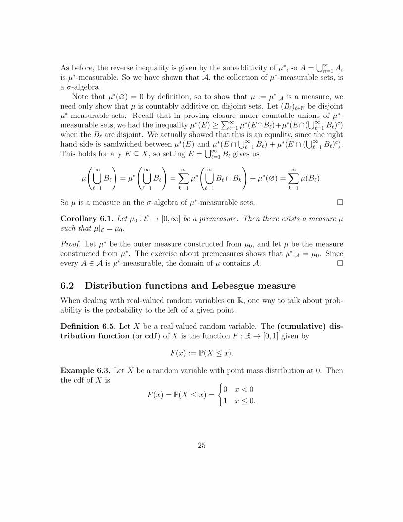
Example 6.3. Let X be a random variable with point mass distribution at 0. Thenthe cdf of X is

F (x) = P(X ≤ x) =

0 x < 0

1 x ≤ 0.

25

This is called the Heaviside step function. It is not continuous, but it is right-continuous.

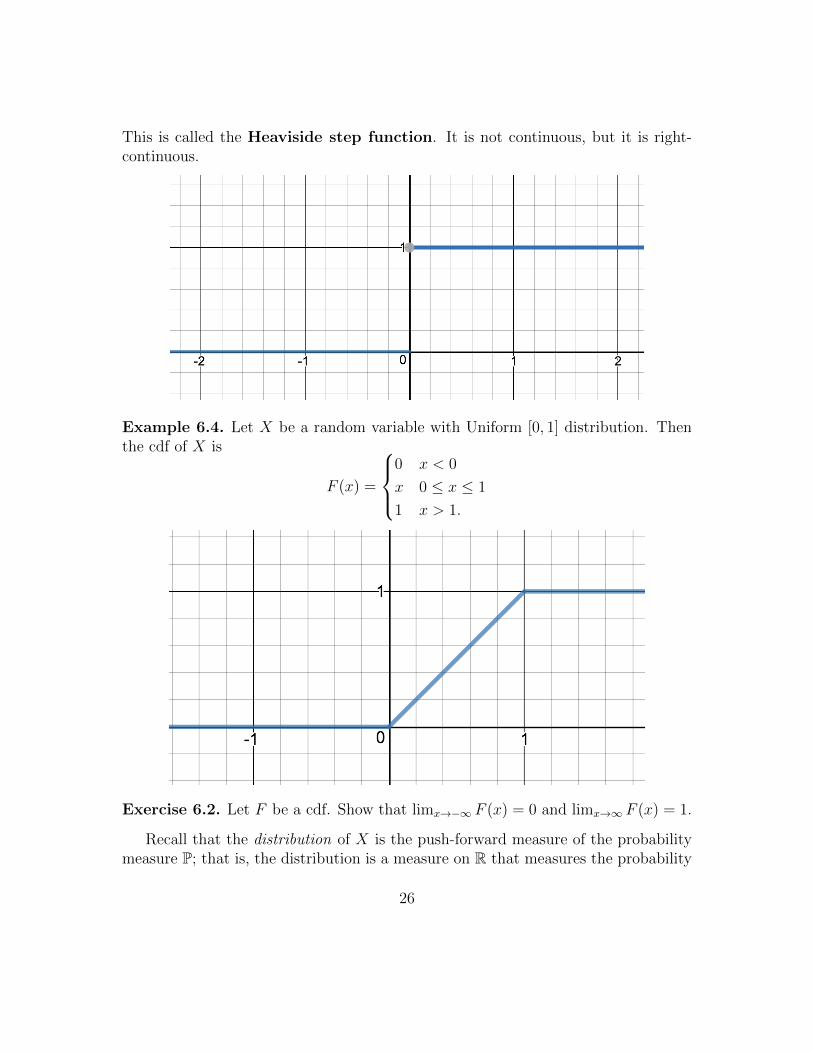
Example 6.4. Let X be a random variable with Uniform [0, 1] distribution. Thenthe cdf of X is

F (x) =

0 x < 0

x 0 ≤ x ≤ 1

1 x > 1.

Exercise 6.2. Let F be a cdf. Show that limx→−∞ F (x) = 0 and limx→∞ F (x) = 1.

Recall that the distribution of X is the push-forward measure of the probabilitymeasure P; that is, the distribution is a measure on R that measures the probability

26

of X taking a value in a given subset of R. This is the same idea, except instead ofencoding the information as a measure, we treat the distribution as a function on R.We will see that these are indeed the same concept.

Why is the cdf of a real-valued random variable important? Consider a randomvariable that takes a value x if some certain event occurs at time x. Then the cdfmeasures the probability that the event has already happened by time x, and 1−F (x)measures the probability that the event will happen after time x.

From an analytic perspective, the study of cumulative distribution functions isthe study of nondecreasing right-continuous functions (limx→a+ F (x) = F (a) for eacha ∈ R). These are central to the idea of Riemann-Stieltjes integration, which willbe a special case of the powerful theory of Lebesgue integration we will develop. Aswith their probability measure counterparts, these functions are closely related tomeasures on the real line.

We have constructed distribution functions from measures on R. Let us now dothe reverse, using the outer measure construction.

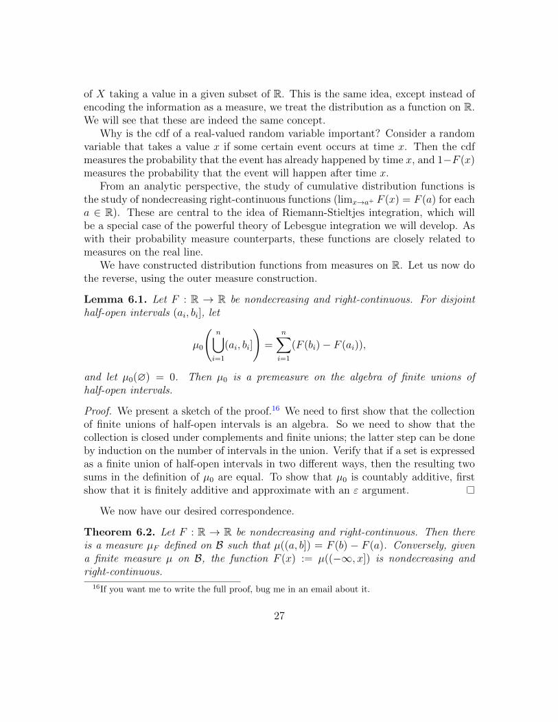
Lemma 6.1. Let F : R → R be nondecreasing and right-continuous. For disjointhalf-open intervals (ai, bi], let

µ0

(n⋃i=1

(ai, bi]

)=

n∑i=1

(F (bi)− F (ai)),

and let µ0(∅) = 0. Then µ0 is a premeasure on the algebra of finite unions ofhalf-open intervals.

Proof. We present a sketch of the proof.16 We need to first show that the collectionof finite unions of half-open intervals is an algebra. So we need to show that thecollection is closed under complements and finite unions; the latter step can be doneby induction on the number of intervals in the union. Verify that if a set is expressedas a finite union of half-open intervals in two different ways, then the resulting twosums in the definition of µ0 are equal. To show that µ0 is countably additive, firstshow that it is finitely additive and approximate with an ε argument.

We now have our desired correspondence.

Theorem 6.2. Let F : R → R be nondecreasing and right-continuous. Then thereis a measure µF defined on B such that µ((a, b]) = F (b) − F (a). Conversely, givena finite measure µ on B, the function F (x) := µ((−∞, x]) is nondecreasing andright-continuous.

16If you want me to write the full proof, bug me in an email about it.

27

Proof. By the lemma, we can construct the measure µF from the premeasure µ0.Since µ0 is defined on a set containing all open intervals, µF is defined on all openintervals. These sets generate B, so since µF is defined on a σ-algebra containingthese sets, µF is defined on at least all of B. Since µF agrees with the premeasureµ0, we have µF ((a, b]) = F (b)− F (a).

Given a finite µ, to show that F is nondecreasing, use the monotonicity of µ. Ifa ≤ b,

F (a) = µ((−∞, a]) ≤ µ((−∞, b]) = F (b).

To show that F is right continuous, use continuity from above.

limx→a+

F (x) = limx→a+

µ((−∞, x]) = µ((∞, a]) = F (a).

In particular, cumulative distribution functions are nondecreasing and right-continuous. So we have shown that distributions and cumulative distribution func-tions are really the same thing for real-valued random variables.

The measures µF are sometimes called Lebesgue-Stieltjes measures. Thesemeasures can be actually defined on a σ-algebra larger than B; this σ-algebra hassome nice properties and will be the subject of exercises at the end of the chapter.17

Exercise 6.3. Show that µF = µG iff F −G is a constant.

Exercise 6.4. Let µ be a measure on B (not necessarily finite). Define a functionF : R → R that is nondecreasing and right-continuous, such that µF = µ on B.(Hint: Let F (0) = 0. In the case that µ is finite, your function may differ from thecdf by a constant.)

We now turn our attention to perhaps the most important (or at least the mostfrequently used) measure: the measure of length on the real line.

Definition 6.6. Lebesgue measure18 λ is the Lebesgue-Stieltjes measure associ-ated to the function F (x) = x.

The Uniform [0, 1] distribution is Lebesgue measure restricted to B[0,1]. So whenwe take an interval (a, b], Lebesgue measure agrees with the value of the premeasureon this interval; that is, λ((a, b]) = F (b)−F (a) = b−a. What about open intervals?Or closed intervals? Or points?

17If you’re reading this, and I haven’t written the exercises yet, send me an email, and bug meuntil I do it.

18For some reason, people always omit articles before mention of Lebesgue measure. There seemsto be an unspoken rule against calling it “the” Lebesgue measure. I have no idea why.

28

Proposition 6.3. Let λ be Lebesgue measure. Then

1. λ(x) = 0 for x ∈ R.

2. If A is countable, λ(A) = 0.

3. For a, b ∈ R with a ≤ b, λ((a, b)) = λ([a, b]) = b− a.

Proof. Properties 2 and 3 follow from the first.

1. Using continuity from above, since x =⋂∞n=1(x− 1/n, x], we have

λ(x) = limk→∞

λ((x− 1/k, x]) = limk→∞

1/k = 0.

2. If A is countable, then A =⋃x∈Ax is a countable union. So by countable

additivity,

λ(A) =∑x∈A

λ(x) =∑x∈A

0 = 0.

3. We already have that λ((a, b]) = b− a. So

λ((a, b)) = λ((a, b])− λ(b) = (b− a)− 0 = b− a,

λ([a, b]) = λ((a, b]) + λ(a) = (b− a) + 0 = b− a.

Corollary 6.2.λ(Q) = 0.

Take a moment to step back and realize how remarkable this is. The rationalnumbers are inifinite and even dense in R, yet our canonical measure on R assignsthem zero measure! Even though the Borel σ-algebra is defined via topologicalproperties of R, Lebesgue measure does not always characterize size in the same wayas the topology does.

Exercise 6.5. Show that for every ε > 0, there is an open, dense subset A ⊆ R suchthat λ(A) < ε. Conclude that an open, dense subset of R need not be R.19

Lebesgue measure is invariant under translations and scales with dilations. Theformer of these properties is an example of a more general property of translation-invariant measures (called Haar measure) on Abelian groups.20

19This is a really interesting problem, especially since it’s so counterintuitive. Many studentsincorrectly believe that open, dense subsets must be the whole space.

20The interplay between the algebraic structure and the measure-theoretic properties is very rich.One of my research interests is exactly this kind of thing: probability on algebraic structures.

29

Proposition 6.4. For r ∈ R, let A+ r := a+ r : a ∈ A and rA := ra : a ∈ A.If A ∈ B, then

1. A+ r, rA ∈ B.

2. λ(A+ r) = λ(A).

3. λ(rA) = |r|λ(A).

Proof. Let A be the collection of sets A in B such that A + r, rA ∈ B for everyr ∈ R. Note that A contains all the open intervals, is closed under complements,and is closed under countable unions. So A is a σ-algebra containing the openintervals, which generate B. So A = B.

The length premeasure on finite unions of half-open intervals is invariant undertranslations and scales with |r| when dilated by r, so the value of the associated outermeasure has these properties, as well. So λ(A+r) = λ(A), and λ(rA) = |r|λ(A).

30

References

[Bas13] R.F. Bass. Real Analysis for Graduate Students. Createspace Ind Pub, 2013.

[Dur10] R. Durrett. Probability: Theory and Examples. Cambridge Series in Statis-tical and Probabilistic Mathematics. Cambridge University Press, 2010.

[Fol13] G.B. Folland. Real Analysis: Modern Techniques and Their Applications.Pure and Applied Mathematics: A Wiley Series of Texts, Monographs andTracts. Wiley, 2013.

31