MARTA LEWICKA, MARIA GIOVANNA MORA AND MOHAMMAD … · 2 MARTA LEWICKA, MARIA GIOVANNA MORA AND...

arX

iv:0

803.

0358

v1 [

mat

h.FA

] 4

Mar

200

8

SHELL THEORIES ARISING AS LOW ENERGY Γ-LIMIT

OF 3D NONLINEAR ELASTICITY

MARTA LEWICKA, MARIA GIOVANNA MORA AND MOHAMMAD REZA PAKZAD

Abstract. We discuss the limiting behavior (using the notion of Γ-limit)of the 3d nonlinear elasticity for thin shells around an arbitrary smooth 2d

surface. In particular, under the assumption that the elastic energy of defor-mations scales like h

4, h being the thickness of a shell, we derive a limitingtheory which is a generalization of the von Karman theory for plates.

Contents

1. Introduction 12. An overview of the main results 33. Convergence of low energy deformations 84. A proof of Theorem 2.1 and some explanations 135. The space of finite strains B and three examples of approximately

robust surfaces 166. The recovery sequence: proofs of Theorems 2.2 and 2.3 217. The convergence of minimizers: proof of Theorem 2.5 268. Appendix A - an approximation theorem on surfaces 309. Appendix B - the Γ-convergence setting 3210. Appendix C - on coercivity of the generalized von Karman functionals

J and J 33References 35

1. Introduction

The derivation of lower dimensional models for thin structures (such as mem-branes, shells, or beams) from the three-dimensional theory, has been one of thefundamental questions since the beginning of research in elasticity [19]. Recently,a novel variational approach through Γ-convergence has lead to the derivation ofa hierarchy of limiting theories. Among other features, it provides a rigorous jus-tification of convergence of three-dimensional minimizers to minimizers of suitablelower dimensional limit energies.

In this paper we discuss shell theories arising as Γ-limits of higher scalings of thenonlinear elastic energy. Given a 2-dimensional surface S, consider a shell Sh ofmid-surface S and thickness h, and associate to its deformation u the scaled per

1991 Mathematics Subject Classification. 74K20, 74B20.Key words and phrases. shell theories, nonlinear elasticity, Gamma convergence, calculus of

variations.

1

http://arxiv.org/abs/0803.0358v1

2 MARTA LEWICKA, MARIA GIOVANNA MORA AND MOHAMMAD REZA PAKZAD

unit thickness three dimensional nonlinear elastic energy Eelastic(u, Sh). We areinterested in the identification of the Γ-limit Iβ of the energies:

h−βEelastic(·, Sh),

as h → 0, for a given scaling β ≥ 0. As mentioned above, this implies conver-gence, in a suitable sense, of minimizers uh of Eelastic (subject to applied forces)to minimizers of two-dimensional energy Iβ , provided E

elastic(uh, Sh) ≤ Chβ .In the case when S is a subset of R2 (i.e. a plate), such Γ-convergence was first

established by LeDret and Raoult [15] for β = 0, then by Friesecke, James andMuller [9, 10] for all β ≥ 2 (see also [24] for results for β = 2 under additionalconditions). In the case of 0 < β < 5/3, the convergence was recently obtainedby Conti and Maggi [5], see also [2]. The regime 5/3 ≤ β < 2 remains open andis conjectured to be relevant for the crumpling of elastic sheets. Other significantresults for plates concern derivation of limit theories for incompressible materials[3, 4, 28], for heterogeneous materials [26] and through establishing convergence ofequilibria, rather than strict minimizers [20, 22].

Much less is known in the general case when S is an arbitrary surface. The firstresult by LeDret and Raoult [16] relates to scaling β = 0 and models membraneshells: the limit I0 depends only on the stretching and shearing produced by thedeformation on the mid-surface S. Another study is due to Friesecke, James, Moraand Muller [8], who analyzed the case β = 2. This scaling corresponds to a flexuralshell model, where the only admissible deformations are those preserving the metricon S. The energy I2 depends then on the change of curvature produced by thedeformation.

All the above mentioned theories (as well as the subsequent results in this pa-per) should be put in contrast with a large body of literature, devoted to deriva-tions starting from three-dimensional linear elasticity (see Ciarlet [1] and referencestherein). Indeed, since thin structures may undergo large rotations even under theaction of very small forces, one cannot assume the small strain condition, on whichthe linear elasticity is based.

The objective of this work is to discuss the limit energies for scalings β ≥ 4,for arbitrary surfaces S. We now give a heuristic overview of our results, whoseprecise formulations will be presented in section 2. If Eelastic(u, Sh) ≈ Chβ , for anyβ > 2, one expects u to be close to a rigid motion R. This argument can be madeprecise by means of the quantitative rigidity estimate due to Friesecke, James andMuller [9] (see also Lemma 8.1). We further demonstrate that the first term in theexpansion of u−R, in terms of h, equals an infinitesimal isometry V . That is, thereis no first order change in the Riemannian metric of S under the displacement V .The corresponding bending energy, given in terms of the first order change in thesecond fundamental form of S, is the Γ-limit Iβ if β > 4 (Theorem 2.3). This limitenergy coincides with the so-called linearly elastic flexural shell model, derived in[1] from the linear elasticity theory. Our result guarantees therefore that, withoutany a priori smallness assumption on the strain, the use of the linearized flexuralshell model is justified whenever the order of magnitude of the per unit thicknessthree-dimensional energy is hβ with β > 4.

When β = 4, also the second order in h change in the metric on S (stretching)contributes to the limiting energy. This change is induced by V , and additionally, byan “approximate second order displacement” w. This last notion involves studying

NONLINEAR SHELL THEORIES 3

the finite strain space. For a similar situation where this space emerges see thediscussion by Sanchez-Palencia [25] and Geymonat and Sanchez-Palencia [11] underthe title of ill-inhibited surfaces, in the context of linear elasticity. In Theorems 2.1and 2.2 we derive the energy functional I4, which can be seen as a generalization ofthe von Karman theory for plates [14], justified in terms of Γ-convergence in [10].Indeed, if S is a plate, then V and w are, respectively, the out-of-plane and thein-plane displacements (modulo a possible in-plane infinitesimal rigid motion).

A particular class of surfaces when I4 simplifies to the bending energy is thehereby introduced class of approximately robust surfaces. We say that S is (ap-proximately) robust if any infinitesimal isometry V can be completed by a secondorder displacement to an (approximate) second order isometry. In other words, Scan always further adjust its deformation, to compensate for the change of metricproduced at second order. As a result, the total stretching of second order is in-significant and the Γ-limit consists only of a bending term (Theorem 2.3). We showthree general examples of approximately robust surfaces: convex surfaces, surfacesof revolution, and developable surfaces without flat parts. An example of a notapproximately robust surface is a plate.

We also address the issue of external forces, depending on the reference configu-ration, namely the dead loads (Theorem 2.5). Under a vanishing average conditionand a suitable scaling of the forces fh applied to Sh, Theorem 2.1 provides aninformation of the deformation of Sh assumed in response to the load. In addi-tion, the appropriate limit force f identifies the set of possible rotations the bodywill undergo. This phenomenon is easily observed: if fh is “compressive”, thenSh prefers to make a large rotation rather than undergoing a compression, and analignment of the infinitesimal isometry V with the force is energetically preferable.

The identification of Γ-limit for any scaling in the range β ∈ (2, 4) and non-flat Sis still open. In analogy with the analysis developed in [10] for plates, the construc-tion of a recovery sequence requires finding an exact isometry of S, coinciding witha given second order isometry. Another direction of study concerns shells, whosemid-surface is inhibited (or infinitesimally rigid). Examples of such are closed orpartially clamped elliptic surfaces. In this case the limit functionals that our theoryyields are identically equal to zero. This suggests looking for higher order termsin the development of the three-dimensional energy in the sense of Γ-convergence.These are subtle issues and we plan to address them in a forthcoming paper.

Acknowledgments. We thank Stefan Muller for helpful discussions. A largepart of this work was carried out while the second author was visiting the Insti-tute for Mathematics and its Applications in Minneapolis (USA), whose supportis gratefully acknowledged. M.L. was partially supported by the NSF grant DMS-0707275. M.G.M. was partially supported by the Italian Ministry of Universityand Research through the project “Variational problems with multiple scales” 2006and by GNAMPA through the project “Problemi di riduzione di dimensione perstrutture elastiche sottili” 2008.

2. An overview of the main results

Let S be a 2-dimensional surface embedded in R3. We assume that S is com-

pact, connected, oriented, and of class C1,1, and that its boundary ∂S is the union


of finitely many (possibly none) Lipschitz continuous curves. Consider a familyShh>0 of thin shells of thickness h around S:

Sh = z = x+ t~n(x); x ∈ S, −h/2 < t < h/2.We will use the following notation: ~n(x) for the unit normal, TxS for the tangentspace, and Π(x) = ∇~n(x) for the shape operator on S, at a given x ∈ S. Theprojection onto S along ~n will be denoted by π, so that:

π(z) = x ∀z = x+ t~n(x) ∈ Sh.

We will assume that h < h0, with h0 > 0 sufficiently small to have π well defined,and so that: 1/2 < |Id + tΠ(x)| < 3/2 for all z as above.

For aW 1,2 deformation of a thin shell uh : Sh −→ R3, we assume that its elastic

energy (scaled per unit thickness) is given by the nonlinear functional:

Eelastic(uh, Sh) =1

h

Sh

W (∇uh),

where the stored-energy density function W is nonnegative and C2 in some openneighborhood O of SO(3), in the space R

3×3 of 3× 3 real matrices. Moreover, Wis assumed to satisfy, for all F ∈ R

3×3 and some C > 0:

W (RF ) =W (F ) ∀R ∈ SO(3),

W (R) = 0 ∀R ∈ SO(3),

W (F ) ≥ Cdist2(F, SO(3)).

Here SO(3) denotes the group of proper rotations. Recall that the tangent spaceto SO(3) at Id is the space of skew-symmetric matrices:

so(3) = F ∈ R3×3; F = −FT .

It is convenient to view uh through their rescalings yh ∈ W 1,2(Sh0 ,R3):

yh(x+ t~n(x)) = uh (x+ th/h0~n(x)) ∀x ∈ S ∀t ∈ (−h0/2, h0/2).The advantage is that all yh have the common domain Sh0 . We are concerned withthe limiting behavior of the energies:

Ih(yh) =1

h

Sh

W (∇uh),

relative to low energy deformations. That is, we want to discuss the limit, ash→ 0, of the functionals Ih/eh, for a given sequence of positive numbers eh, whichwe assume to satisfy:

(2.1) limh→0

eh/h4 = κ2 <∞.

With this in mind, define the related scaled average displacement:

(V h[yh])(x) =h√eh

h0/2

−h0/2

yh(x + t~n)− x dt.

Since we will frequently deal with such vector fields V ∈ W 1,2(S,R3) on the surface,we introduce the following notation. By sym ∇V (x) we mean a bilinear form onTxS given by: (sym ∇V (x)τ)η = 1

2 [(∂τV (x))η + (∂ηV (x))τ ], for all τ, η ∈ TxS.

Also, given a matrix field A ∈ L2(S,R3×3), by Atan(x) we denote the tangentialminor of A at x ∈ S, that is [(A(x)τ)η]τ,η∈TxS .


Our first main result is the following:

Theorem 2.1. Assume (2.1) and let uh ∈ W 1,2(Sh,R3) be a sequence of defor-mations such that the sequence of scaled energies 1

eh Ih(yh) is bounded. Then

there exist rigid motions of R3, given through proper rotations Qh ∈ SO(3) and

translations ch ∈ R3 such that for the normalized deformations:

yh(x + t~n) = (Qh)T yh(x+ t~n)− ch

the following holds.

(i) yh converge in W 1,2(Sh0) to π.(ii) V h[yh] converge (up to a subsequence) in W 1,2(S) to some vector field V ∈

W 2,2(S,R3) with skew-symmetric gradient, that is:

(2.2) ∂τV (x) = A(x)τ ∀τ ∈ TxS, a.e. x ∈ S

for some matrix field A ∈ W 1,2(S,R3×3) such that:

(2.3) A(x) ∈ so(3) ∀x ∈ S.

(iii) 1h sym ∇V h[yh] converge (up to a subsequence) weakly in L2(S) to somesymmetric matrix field Btan on S.

(iv) There holds:

lim infh→0

1

ehIh(yh) ≥ I(V,Btan),

where:(2.4)

I(V,Btan) =1

2

S

Q2

(

x,Btan − κ

2(A2)tan

)

+1

24

S

Q2 (x, (∇(A~n)−AΠ)tan) .

The following quadratic, nondegenerate forms are of relevance here:

(2.5) Q3(F ) = D2W (Id)(F, F ), Q2(x, Ftan) = minQ3(F ); (F − F )tan = 0.The form Q3 is defined for F ∈ R

3×3, while Q2(x, ·), for a given x ∈ S is definedon tangential minors Ftan of such matrices. Both forms Q3 and all Q2(x, ·) arepositive definite and depend only on the symmetric parts of their arguments (see[9]).

Theorem 2.1 will be proved in sections 3 and 4. One of the crucial ingredientsis a result on approximating large deformations [9]. For completeness, we sketchits proof, in the setting of shells, in Appendix A. We also note that because ofthe non trivial geometry of the shell, the limiting energy I, in general, exhibits adependence on the point x ∈ S, although the three-dimensional configuration ishomogeneous.

Our second main result concerns the possibility of recovering the functionalI(V,Btan) in (2.4) (or its components), as the limit of scaled energies 1

ehIh(yh),

for some sequence of deformations. For this, define the finite strain displacementspace:

B =

limh→0

sym ∇wh; wh ∈W 1,2(S,R3)

,

where limits are taken in L2(S) (clearly, both the weak and the strong convergencesyield the same B). We then have:


Theorem 2.2. Assume (2.1). For every V ∈ W 2,2(S,R3) satisfying (2.2) and(2.3), and every Btan ∈ B, there exists a sequence of deformations uh ∈W 1,2(Sh,R3)such that:

(i) yh converge in W 1,2(Sh0) to π.(ii) V h[yh] converge in W 1,2(S) to V .(iii) 1

h sym ∇V h[yh] converge in L2(S) to Btan.(iv) Recalling the definition (2.4) one has:

limh→0

1

ehIh(yh) = I(V,Btan).

The form of the limiting energy functional I simplifies, when the space B is largeenough to choose Btan so that the first term in (2.4) vanishes. That is, we call S“approximately robust” if for every V ∈ W 2,2(S,R3) satisfying (2.2) (2.3), one has(A2)tan ∈ B. Then we have:

Theorem 2.3. Assume (2.1). Let κ = 0 or let S be approximately robust. Thenfor every V ∈ W 2,2(S,R3) satisfying (2.2) and (2.3), there exists a sequence ofdeformations uh ∈W 1,2(Sh,R3) such that (i) and (ii) of Theorem 2.2 hold. More-over:

limh→0

1

ehIh(yh) = I(V ),

where

(2.6) I(V ) =1

24

S

Q2

(

x,(

∇(A~n)−AΠ)

tan

)

.

Theorems 2.2 and 2.3 will be proved in section 6. In section 5 we discuss thespace B and approximately robust surfaces. In particular, we shall see that convexsurfaces, surfaces of revolution, and non-flat developable surfaces are approximatelyrobust.

Theorems 2.1 and 2.2 (or 2.3) can be summarized (although they provide moreinformation than the below statement), using the language of Γ-convergence. Forcompleteness, the following result will be presented in Appendix B.

Corollary 2.4. Assume (2.1).

(i) Define a sequence of functionals:

Fh :W 1,2(Sh0 ,R3)×W 1,2(S,R3)× L2(S,R2×2) −→ R

Fh(yh, V h, Bhtan) =

1

ehIh(yh) if V h = V h[yh] and Bh

tan = 1h sym ∇V h,

+∞ otherwise.

Then Fh Γ-converge, as h→ 0, to the following functional:

F(y, V,Btan) =

I(V,Btan) if y = π, V ∈W 2,2 satisfies (2.2), (2.3),and Btan ∈ B,

+∞ otherwise.

(ii) Assume that κ = 0 or let S be approximately robust. Define the functionals:

Fh :W 1,2(Sh0 ,R3)×W 1,2(S,R3) −→ R

Fh(yh, V h) =

1

ehIh(yh) if V h = V h[yh]

+∞ otherwise.


Then Fh Γ-converge, as h→ 0, to the functional:

F(y, V ) =

I(V ) if y = π and V ∈W 2,2 satisfies (2.2), (2.3),+∞ otherwise.

All statements above remain valid if the product spaces (the domains of functionals

Fh, Fh) are equipped with the weak (instead of strong) topology.

We further consider a sequence of forces fh ∈ L2(Sh,R3), acting on thin shellsSh. For simplicity, we assume that:

fh(x + t~n(x)) = h√eh det (Id + tΠ(x))−1 f(x),

where f ∈ L2(S,R3) is normalized so that:

(2.7)

S

f = 0.

Define m to be the maximized action of force f on S over all rotations of S, andlet M be the corresponding set of maximizers:

(2.8) M =

Q ∈ SO(3);

S

f(x) · Qx dx = m = maxQ∈SO(3)

S

f ·Qx

.

The total energy functional on Sh is given through:

Jh(yh) = Ih(yh) +mh − 1

h

Sh

fhuh,

where mh = h√ehm.

Theorem 2.5. Assume (2.1) and (2.7). Then:

(i) For every small h > 0 one has:

0 ≥ inf

1

ehJh(yh); uh ∈ W 1,2(Sh,R3)

≥ −C.

(ii) If uh ∈ W 1,2(S,R3) is a minimizing sequence of 1ehJh, that is:

(2.9) limh→0

(

1

ehJh(yh)− inf

1

ehJh

)

= 0,

then there exists Qh ∈ SO(3) and ch ∈ R3 such that for the normalized

deformations yh = (Qh)T yh − ch the convergences of Theorem 2.1 (i) (ii)and (iii) hold. The convergence of (a subsequence of) 1

h sym∇V h[yh] to

Btan in (iii) is strong in L2(S).Moreover, the set of accumulation points of Qh is contained within M.

Any limit (V,Btan, Q) minimizes the functional:

J(V,Btan, Q) = I(V,Btan)−

S

f · QV,

over all V ∈W 2,2(S,R3) satisfying (2.2) (2.3), all Btan ∈ B and Q ∈ M.(iii) If κ = 0 in (2.1), or if S is approximately robust, then for any minimiz-

ing sequence as in (2.9), we obtain convergences of yh, V h[yh] and Qh asdescribed in (ii) above, and the limit (V, Q) minimizes the functional:

J(V, Q) = I(V )−

S

f · QV

over all V ∈W 2,2(S,R3) satisfying (2.2) (2.3) and all Q ∈ M.


In section 7, we prove Theorem 2.5 and explain the significance of the set M inthe setting of dead loads.

The lower bound on the functionals J and J , as well as attainment of theirinfima, can be proved independently, under conditions (2.7) and:

(2.10)

S

f(x) · QFx dx = 0 ∀Q ∈ M ∀F ∈ so(3).

Here M is any closed, nonempty subset of SO(3). When M has the form (2.8),then (2.10) follows from (2.8) and can be seen as its linearization. This analysiswill be carried out in Appendix C.

3. Convergence of low energy deformations

In this section we derive some bounds on families of vector mappings uhh>0,defined on Sh, under the assumption of smallness on their energy. In what follows,by C we denote an arbitrary positive constant, depending on the geometry of S butnot on h or the vector mapping under consideration. In all proofs, the convergencesare understood up to a subsequence, unless stated otherwise.

We will work under the following hypothesis:

(H)

A sequence of vector mappings uh ∈ W 1,2(Sh,R3) and a sequence ofpositive numbers eh satisfy, for small h > 0:

(i)1

h

Sh

W (∇uh) ≤ Ceh,

(ii) limh→0

eh/h2 = 0.

As for the flat case in [10], the first crucial step is the following approximationresult:

Lemma 3.1. For each uh as in (H) there exist a matrix field Rh ∈ W 1,2(S,R3×3)such that:

Rh(x) ∈ SO(3) ∀x ∈ S,

and a matrix Qh ∈ SO(3) such that:

(i) ‖∇uh −Rhπ‖L2(Sh) ≤ Ch1/2√eh,

(ii) ‖∇Rh‖L2(S) ≤ Ch−1√eh,

(iii) ‖(Qh)TRh − Id‖Lp(S) ≤ Ch−1√eh, for all p ∈ [1,∞),

The proof follows from Lemma 8.1 given in Appendix A, in view of:

E(uh, Sh) =

Sh

dist2(∇uh, SO(3)) ≤ C

Sh

W (∇uh) ≤ Cheh

so that limh→0 h−3E(uh, Sh) = 0 by hypothesis (H).

Lemma 3.2. Assume (H) and let Rh, Qh be given as in Lemma 3.1. There holds:

(i) limh→0

(Qh)TRh = Id, in W 1,2(S) and in Lp(S).

Moreover, there exists a W 1,2 skew-symmetric matrix fields A : S −→ so(3) suchthat:

(ii) limh→0

h√eh

(

(Qh)TRh − Id)

= A, weakly inW 1,2(S) and (strongly) in Lp(S).


(iii) limh→0

h2

ehsym

(

(Qh)TRh − Id)

=1

2A2, in Lp(S).

In (ii) and (iii) convergence is up to a subsequence (that we do not relabel). In (i),(ii), and (iii) the appropriate convergence holds for all p ∈ [1,∞).

Proof. The convergences in (i) follow from Lemma 3.1 in view of (H). To prove(ii), notice that the sequence:

Ah =h√eh

(

(Qh)TRh − Id)

is bounded in W 1,2(S) and so it has a weakly converging subsequence. By compactembedding of W 1,2(S) into Lp(S) the convergence is strong in Lp(S). One has:

Ah + (Ah)T =h√eh

(

(Qh)TRh + (Rh)TQh − 2Id)

= −√eh

h(Ah)T · Ah.

The latter converges to 0 in Lp(S), and therefore the limit matrix field A is skew-symmetric. The above equality proves as well that:

limh→0

h√eh

sym Ah =1

2A2

in Lp(S), which implies (iii).

Recall the rescaling:

yh(x+ t~n(x)) = uh (x+ th/h0~n(x)) ∀x ∈ S ∀t ∈ (−h0/2, h0/2),

so that yh ∈ W 1,2(Sh0 ,R3). Also, define:

∇hyh(x+ t~n(x)) = ∇uh (x+ th/h0~n(x))

By a straightforward calculation we obtain:

Proposition 3.3. For each x ∈ S, t ∈ (−h0/2, h0/2) and τ ∈ TxS there hold:

∂τyh(x+ t~n) = ∇hy

h (x+ t~n) (Id + th/h0Π(x)) (Id + tΠ(x))−1τ

∂~nyh(x+ t~n) =

h

h0∇hy

h (x+ t~n)~n(x).

Moreover, for Ih(yh) = 1h

Sh W (∇uh) one has:

Ih(yh) =1

h0

Sh0

W (∇hyh(x + t~n)) · det

[

(Id + th/h0Π) (Id + tΠ)−1]

=

S

h0/2

−h0/2

W (∇hyh(x+ t~n)) · det [Id + th/h0Π(x)] dt dx.

Also, directly from Lemma 3.1 (i) and Lemma 3.2 (ii) there follows:

Proposition 3.4. Assume (H). Then:

(i) ‖∇hyh −Rhπ‖L2(Sh0) ≤ C

√eh.

(ii) limh→0

h√eh

(

(Qh)T∇hyh − Id

)

= Aπ, in L2(Sh0) up to a subsequence.


We will consider the corrected by rigid motions deformations yh ∈ W 1,2(Sh0 ,R3)and averaged displacements V h ∈W 1,2(S,R3):

yh = (Qh)T yh − ch, V h = V h[yh] =h√eh

h0/2

−h0/2

yh(x+ t~n)− x dt,

where ch =

S

h0/2

−h0/2(Qh)T yh − x dt dx, so that

S Vh = 0.

Lemma 3.5. Assume (H). Then:

(i) limh→0

yh = π, in W 1,2(Sh0).

(ii) limh→0

V h = V, in W 1,2(S) up to a subsequence.

The vector field V in (ii) has regularityW 2,2(S,R3) and it satisfies ∂τV (x) = A(x)τfor all τ ∈ TxS. The W 1,2 skew-symmetric matrix field A : S −→ so(3) is as inLemma 3.2.

Proof. 1. In view of Proposition 3.3 and Proposition 3.4 we have:∥

∥∇tanyh −

(

(Qh)TRh)

tan· (Id + th/h0Π)(Id + tΠ)−1

∥

∥

L2(Sh0 )≤ C

√eh

∥

∥∂~nyh∥

∥

L2(Sh0 )≤ Ch‖∇hy

h‖L2(Sh0 ) ≤ Ch.(3.1)

To prove convergence of V h, consider:

∇V h(x) =h√eh

h0/2

−h0/2

∇tanyh(x + t~n)(Id + tΠ)− Id dt

=h√eh

h0/2

−h0/2

(

∇tanyh −

(

(Qh)TRh)

tan(Id + tΠ)−1

)

(Id + tΠ) dt

+h√eh

(

(Qh)TRh(x)− Id)

tan.

(3.2)

We see that by (3.1) the first term in the right hand side above converges to 0 inL2(Sh0), as h → 0. The second term converges, up to a subsequence, to Atan byLemma 3.2 (ii). Therefore ∇V h converges to Atan in L2(S) and since

S Vh = 0,

we may use Poincare inequality on S to deduce (ii).2. To prove (i), notice that by (3.1) and Lemma 3.2 we obtain the following

convergences in L2(Sh0):

limh→0

∇tanyh = (Id + tΠ)−1 = ∇tanπ,

limh→0

∂~nyh = 0.

Therefore ∇yh converges to ∇π in L2(Sh0).Since the sequence V h is bounded in L2(S), it also follows that:

(3.3) limh→0

∥

∥

∥

∥

∥

h0/2

−h0/2

yh − π dt

∥

∥

∥

∥

∥

L2(S)

= 0.

Now, let g(x+ t~n) = |det (Id+ tΠ(x))|−1. Consider the two terms in the right handside of:

‖yh−π‖L2(Sh0 ) ≤∥

∥

∥

∥

(yh − π)−

Sh0

(yh − π) · g

Sh0g

∥

∥

∥

∥

L2(Sh0 )

+

∣

∣

∣

∣

Sh0

(yh − π) · g

Sh0g

∣

∣

∣

∣

.


The first term can be bounded by means of the weighted Poincare inequality, by‖∇(yh − π)‖L2(Sh0 ) and therefore it converges to 0 as h → 0. The second term

converges to 0 as well, in view of (3.3) and:

∣

∣

∣

∣

Sh0

(yh − π) · g∣

∣

∣

∣

=

∣

∣

∣

∣

∣

S

h0/2

−h0/2

yh − π dt dx

∣

∣

∣

∣

∣

≤ C

∥

∥

∥

∥

∥

h0/2

−h0/2

yh − π dt

∥

∥

∥

∥

∥

L2(S)

.

This justifies convergence of yh to π in L2(Sh0) and ends the proof of (i).

Towards the proof of Theorem 2.1, we need to consider the following sequenceof matrix fields on Sh0 :

Gh =1√eh

(

(Rh)T∇hyh − Id

)

.

In view of Proposition 3.4 (i), 2symGh is the√eh order term in the expansion of

the nonlinear strain (∇uh)T∇uh, at Id. This expression will also play a major role

in the expansion of the energy density at Id: W (∇hyh) =W (Id +

√ehGh).

Lemma 3.6. Assume (H). Then the sequence Gh as above has a subsequence,converging weakly in L2(Sh0) to a matrix field G. The tangential minor of G is,moreover, affine in the ~n direction. More precisely:

∀τ ∈ TxS G(x + t~n)τ = G0(x)τ +t

h0·(

∇(A~n)(x) −AΠ(x))

τ,

where G0(x) =

h0/2

−h0/2

G(x+ t~n) dt.

Proof. 1. The sequence Gh is bounded in L2(Sh0) by Proposition 3.4 (i). There-fore it has a subsequence (which we do not relabel) converging weakly to someG.

For a fixed s > 0, consider now the sequence of vector fields f s,h ∈ W 1,2(Sh0 ,R3):

f s,h(x+t~n) =1

s√eh

[(

h0yh(x+(t+s)~n)−h(x+(t+s)~n)

)

−(

h0yh(x+t~n)−h(x+t~n)

)]

We claim that f s,h converges in L2(Sh0) (up to a subsequence) to (A~n)π as h→ 0.Indeed, using Proposition 3.3 one has:

f s,h(x+ t~n) =1√eh

t+s

t

(

h0∂~nyh(x+ σ~n)− h~n

)

dσ

=h√eh

t+s

t

(

(Qh)T∇hyh(x+ σ~n)− Id

)

~n dσ,

and the convergence follows by Proposition 3.4 (ii).

2. We claim that this convergence is actually weak in W 1,2(Sh0). First, noticethat the normal derivatives converge to 0 in L2(Sh0) by Proposition 3.4 (ii):

∂~nfs,h(x+ t~n) =

h

s√eh

(Qh)T(

∇hyh(x+ (t+ s)~n)−∇hy

h(x+ t~n))

~n(x).


We now find the weak limit of the tangential gradients of f s,h. By Proposition 3.3there holds, for all τ ∈ TxS:

∂τfs,h(x + t~n) =

1

s√eh

(

h0∇yh(x + (t+ s)~n)(Id + (t+ s)Π)(Id + tΠ)−1

− h0∇yh(x+ t~n)− hsΠ(Id + tΠ)−1)

τ

=h0

s√eh

(Qh)T(

∇hyh(x+ (t+ s)~n)−∇hy

h(x+ t~n))

(Id + th/h0Π)(Id + tΠ)−1τ

+h

s√eh

(

(Qh)T∇hyh(x+ (t+ s)~n)− Id

)

sΠ(Id + tΠ)−1τ.

By Proposition 3.4 (ii), the second term in the right hand side above:

h√eh

(

(Qh)T∇hyh(x+ (t+ s)~n)− Id

)

Π(Id + tΠ)−1

converges in L2(Sh0) to AΠ(Id + tΠ)−1.On the other hand, the first term equals to:

h0s(Qh)TRh

(

Gh(x+ (t+ s)~n)−Gh(x+ t~n))

(Id + th/h0Π)(Id + tΠ)−1

and by Lemma 3.2 (i) it converges weakly in L2(Sh0) to

h0s

(

G(x + (t+ s)~n)−G(x + t~n))

(Id + tΠ)−1.

This establishes the (weak) convergence of f s,h in W 1,2(Sh0).

3. Equating the weak limits of tangential derivatives, we obtain, for every τ ∈TxS:

∂τ (A~n)(x) · (Id + tΠ)−1 =h0s

(

G(x + (t+ s)~n)−G(x + t~n))

(Id + tΠ)−1τ

+AΠ(Id + tΠ)−1τ.

This proves the lemma.

Finally, we have the following bound for convergence of the scaled energies Ih:

Lemma 3.7. Assume (H). Then:

lim infh→0

1

ehIh(yh) ≥ 1

2

S

Q2 (x, (sym G0)tan) +1

24

S

Q2 (x, (∇(A~n)−AΠ)tan) .

Proof. By the frame invariance property of W we have:

W (∇hyh) =W ((Rh)T∇hy

h) =W (Id +√ehGh).

Consider the sets Ωh = x ∈ Sh0 ; (eh)1/4|Gh(x)| ≤ 1. Clearly the sequence ofcharacteristic functions χΩh

converges to 1 in L1(Sh0), as (eh)1/4Gh convergespointwise to 0. SinceW is C2 in a neighborhood of Id, then by the above calculation,


in Ωh (for h sufficiently small) there holds:

1

ehW (∇hy

h) =1

eh1

2D2W (Id)(

√ehGh,

√ehGh)

+

1

0

(1− s)[

D2W (Id + s√ehGh)−D2W (Id)

]

ds (Gh, Gh)

=1

2Q3(G

h) + o(1)|Gh|2.

(3.4)

Above o(1) is the Landau symbol denoting any quantity uniformly converging to0, as h→ 0. In view of Proposition 3.3 we now obtain:

lim infh→0

1

ehIh(yh) ≥ lim inf

h→0

1

eh

S

h0/2

−h0/2

χΩhW (∇hy

h)det [Id + th/h0Π] dt dx

= lim infh→0

S

h0/2

−h0/2

χΩh

1

ehW (∇hy

h) dt dx

= lim infh→0

1

2

S

h0/2

−h0/2

Q3

(

sym (χΩhGh)

)

+ o(1)

Sh0

|Gh|2

≥ 1

2

S

h0/2

−h0/2

Q3(sym G).

The last inequality follows from positive definiteness of Q3 on symmetric matrices,and the fact that χΩh

Gh converges weakly to G, in L2(Sh0).By the definition of Q2 and by Lemma 3.6 we get:

1

2

S

h0/2

−h0/2

Q3(sym G) =1

2

S

h0/2

−h0/2

Q2 (x, (sym G)tan)

=1

2

[

S

h0/2

−h0/2

Q2 (x, (sym G0)tan) +

S

h0/2

−h0/2

t2

h20Q2 (x, (∇(A~n)−AΠ)tan)

]

,

which proves the result.

4. A proof of Theorem 2.1 and some explanations

To complete the proof of Theorem 2.1, in view of Lemma 3.5 and Lemma 3.7,it remains to understand the structure of the admissible matrices G0. This is thecontent of the next lemma.

In addition to the hypothesis (H), we now also assume the existence of the finitelimit:

(4.1) κ = limh→0

√eh/h2 <∞.

When eh ≈ hβ, this corresponds to the case β ≥ 4, with κ > 0 for β = 4 and κ = 0for β > 4.

Lemma 4.1. Assume (H) and (4.1). Let G0 be the matrix field on S, as in Lemma3.6. Then we have the following convergence, up to a subsequence, weakly in L2(S):

(4.2) limh→0

1

hsym ∇V h =

(

sym G0 +κ

2A2)

tan,

where the subscript tan denotes, as usual, the tangential minor of a given matrixfield on S.


Proof. We use the formula (3.2) to calculate 1h sym ∇V h. The last term in the right

hand side gives:

1√eh

sym(

(Qh)TRh − Id)

tan=

√eh

h2h2

ehsym

(

(Qh)TRh − Id)

tan,

which converges in L2(S) to κ/2(A2)tan by Lemma 3.2 (iii).To treat the first term in the right hand side of (3.2), notice that for every

τ ∈ TxS:

1√eh

[

h0/2

−h0/2

∇yh(x+ t~n)(Id + tΠ)− (Qh)TRh(x) dt

]

τ

=1√eh

(Qh)T

[

h0/2

−h0/2

∇hyh(x + t~n)−Rh(x) dt+

h0/2

−h0/2

th/h0∇hyhΠ dt

]

τ

=1√eh

(Qh)TRh(x)

[

h0/2

−h0/2

(Rh)T∇hyh − Id dt

]

τ

+h/h0√eh

(Qh)T

[

h0/2

−h0/2

t(

∇hyh −Rhπ

)

dt

]

Π(x)τ,

where we used Proposition 3.3. Now, the second term in the right hand side aboveconverges in L2(S) to 0, by Proposition 3.4 (i). Further, the matrix in the firstterm equals to:

(Qh)TRh(x)

h0/2

−h0/2

Gh(x+ t~n) dt,

and by Lemma 3.2 (i) and Lemma 3.6, it converges weakly in L2(S) to G0. Thiscompletes the proof.

We now comment on the regularity and role of various quantities containing Vand A, intrinsically related to the geometry of the problem.

Remark 4.2. Notice first that if a vector field V ∈ W 2,2(S,R3) has skew-symmetricgradient:

τ · ∂τV (x) = 0 ∀τ ∈ TxS,

then it uniquely determines a W 1,2 matrix field A : S −→ so(3) by:

∀τ ∈ TxS Aτ = ∂τV,

A~n = Π · Vtan −∇tan(V ~n).(4.3)

Regarding the regularity, write V as the sum of its tangential and normal com-ponents, to obtain:

V = Vtan + (V ~n)~n, sym ∇V = sym ∇Vtan + (V ~n)Π.

Hence, assuming sufficient regularity of S (say, S is C3,1 up to its boundary) itfollows that sym ∇Vtan = −(V ~n)Π ∈ W 2,2(S,R2×2). Using the same calculationsas in [1] page 119, we may deduce that the tangential component Vtan enjoys higherregularity than the vector field V . Namely, Vtan ∈ W 3,2(S,R3) and:

‖Vtan‖W 3,2(S) ≤ C(

‖Vtan‖W 1,2(S) + ‖V ~n‖W 2,2(S)

)

.


By Korn’s inequality, one can replace the W 1,2 norm of Vtan by a term of the order‖Vtan‖L2 + ‖sym ∇Vtan‖L2, so that we finally obtain:

‖Vtan‖W 3,2(S) ≤ C(

‖Vtan‖L2(S) + ‖V ~n‖W 2,2(S)

)

.

For an elementary derivation of Korn’s inequality on S from Korn’s inequality onopen sets, see e.g. [17].

In the same manner, one can prove the following useful bound, valid under C2,1

regularity of S:

(4.4) ‖Vtan‖W 2,2(S) ≤ C(

‖Vtan‖L2(S) + ‖V ~n‖W 1,2(S)

)

.

Remark 4.3. 1. The (scaled) t - derivative of Gτ , which is also the argument of

the second term in the definition of I (and I), may be written as:(

∇(A~n)−AΠ)

τ =[

(

∇(A~n)−AΠ)

τ]

tan= (∂τA)~n.

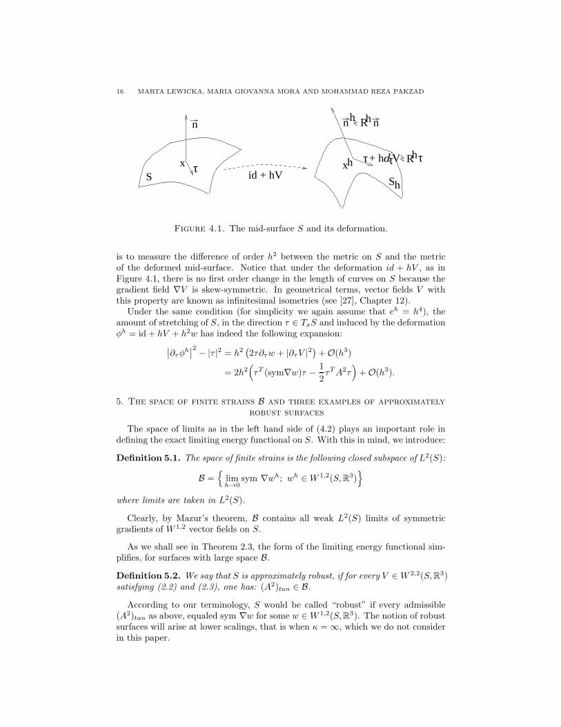
This expression measures the difference of order h between the shape operator Πon S and the shape operator Πh of the deformed surface Sh = (id + hV )(S) (seeFigure 4.1). To see this, let x ∈ S and let τ1, τ2 ∈ TxS be such that ~n(x) = τ1 × τ2.The tangent map of the deformation φh(x) = x + hV (x) equals Id + hA, and weobtain the following expansion of the (scaled) normal vector ~nh to Sh at the pointφh(x):

~nh =(

∂τ1φh × ∂τ2φ

h)

(x) = ~n(x) + h(τ1 × ∂τ2V + ∂τ1V × τ2) +O(h2)

= ~n+ hA~n+O(h2),

where we used the Jacobi identity for vector product and the fact that A ∈ so(3).Note that |~nh| = 1 +O(h2) and therefore

Πh(Id + hA)τ = ∂τ

(

~nh

|~nh|

)

= ∂τ~nh +O(h2).

Hence the amount of bending of S, in the direction of τ ∈ TxS, can be estimatedby:

(Id + hA)−1Πh(Id + hA)τ −Πτ = (Id + hA)−1(∂τ~nh +O(h2))−Πτ

= (Id + hA)−1(

(Id + hA)Πτ + h(∂τA)~n+O(h2))

−Πτ

= (Id− hA)h(∂τA)~n+O(h2) = h(∂τA)~n+O(h2).

A closely related heuristics is the following. By Proposition 3.4 (for simplicity, weassume here that eh = h4) the tangent map ∇uh(x), at x ∈ S, is approximately arotation Rh(x) ∈ SO(3). Hence, ~nh ≈ Rh~n. Assuming that limQh = Id, we maythink that Rh(x) ≈ Id+hA(x). The difference of the shape operators on Sh and Ssatisfies:

(Rh)T∇~nh −Π ≈ (Id + hAT )(

Π+ h∇tan(A~n))

−Π

≈ h∇tan(A~n) + hATΠ = h(

∇(A~n)−AΠ)

tan.

2. In turn, the role of the first term in the definition of I:

(sym G0)tan = limh→0

1

hsym ∇V h − κ

2(A2)tan,


n nRhnh

Sh

xh τ τRhdτ+ h V

id + hVSx τ

Figure 4.1. The mid-surface S and its deformation.

is to measure the difference of order h2 between the metric on S and the metricof the deformed mid-surface. Notice that under the deformation id + hV , as inFigure 4.1, there is no first order change in the length of curves on S because thegradient field ∇V is skew-symmetric. In geometrical terms, vector fields V withthis property are known as infinitesimal isometries (see [27], Chapter 12).

Under the same condition (for simplicity we again assume that eh = h4), theamount of stretching of S, in the direction τ ∈ TxS and induced by the deformationφh = id + hV + h2w has indeed the following expansion:

∣

∣∂τφh∣

∣

2 − |τ |2 = h2(

2τ∂τw + |∂τV |2)

+O(h3)

= 2h2(

τT (sym∇w)τ − 1

2τTA2τ

)

+O(h3).

5. The space of finite strains B and three examples of approximately

robust surfaces

The space of limits as in the left hand side of (4.2) plays an important role indefining the exact limiting energy functional on S. With this in mind, we introduce:

Definition 5.1. The space of finite strains is the following closed subspace of L2(S):

B =

limh→0

sym ∇wh; wh ∈W 1,2(S,R3)

where limits are taken in L2(S).

Clearly, by Mazur’s theorem, B contains all weak L2(S) limits of symmetricgradients of W 1,2 vector fields on S.

As we shall see in Theorem 2.3, the form of the limiting energy functional sim-plifies, for surfaces with large space B.

Definition 5.2. We say that S is approximately robust, if for every V ∈W 2,2(S,R3)satisfying (2.2) and (2.3), one has: (A2)tan ∈ B.

According to our terminology, S would be called “robust” if every admissible(A2)tan as above, equaled sym ∇w for some w ∈W 1,2(S,R3). The notion of robustsurfaces will arise at lower scalings, that is when κ = ∞, which we do not considerin this paper.


Remark 5.3. An equivalent construction of B is the following. Define the linearspace of finite strain displacements:

W =W 1,2(S,R3)/w ∈W 1,2; sym ∇w = 0.

It can be normed by ‖[w]‖W = ‖sym ∇w‖L2(S). Then (B, ‖ · ‖L2(S)) is linearly

isometric to the completion W of (W , ‖ ·‖W), so that the elements of B can be seenas generalized symmetric gradients of elements of W .

Such construction is used in [11] or in [1] in the context of derivation of membranetheories from linear elasticity. Note the different regularity of the kernels consideredin [11] and the related explanations in [1], page 262.

Remark 5.4. In general, it is complicated to directly determine the exact form ofB or W . The crucial step in identifying W is finding the optimal norm ‖ · ‖o forwhich a Korn-Poincare type inequality

(5.1) inf

‖u− w‖o; w ∈W 1,2, sym ∇w = 0

≤ C‖sym∇u‖L2(S)

holds with a uniform constant C, for all u ∈ W 1,2(S,R3). Unlike in the case oftangent vector fields, this optimal norm is usually weaker than L2. The reason isthat the boundedness of the left hand side in:

sym ∇wh = sym ∇whtan + (wh~n)Π

does not, in general, imply L2 boundedness of both terms in the right hand side.This is the case, for example, when S is (a piece of) a cylinder S1 × [−1/2, 1/2].

Let τ1 and τ2 be the tangent unit vector fields, respectively orthogonal and parallelto the axis x3 of the cylinder. One can show that there exists a sequence [wh] ∈ Wconverging in W , such that for any choice of representatives wh ∈ W 1,2(S,R3),the norms ‖whτ1‖L2(S) and ‖wh~n‖H−1(S) blow up. However, this is the worst casescenario, and one has:

W =

v ∈ D′(S,R3); vτ1 ∈ H−1(S), vτ2 ∈ L2(S), v~n ∈ H−2(S),

sym ∇v ∈ L2(S), 1/2

−1/2

x3(v~n) ≡ const,

1/2

−1/2

v~n ≡ const,

S

vτ1 =

S

vτ2 =

S

x3(vτ1) = 0

.

In this particular case, however, as we will see below, W is isometric to the spaceof all symmetric L2 matrix fields Btan on S.

Remark 5.5. Flat surfaces S ⊂ R2 are not approximately robust. Indeed:

B =

sym ∇w; w ∈W 1,2(S,R3)

=

Btan ∈ L2(S,R2×2); BTtan = Btan, curl

T curl Btan = 0

.

On the other hand, given V ∈ W 2,2(S,R3) satisfying (2.2) and (2.3), one has(A2)tan ∈ B if and only if V 3 = V ~n solves the degenerate Monge-Ampere equation:det∇2(V 3) = 0 (see [10]).


A particular class of surfaces which are approximately robust are surfaces forwhich:

(5.2) B =

Btan ∈ L2(S,R2×2); BTtan = Btan

.

As we show below, three main examples of such surfaces are: convex surfaces,surfaces of revolution, and developable surfaces without flat regions.

Lemma 5.6. Assume that S is a simply connected, compact surface of class C2,1

with C1 boundary, and that its shape operator Π is strictly positive (or strictlynegative) definite up to the boundary:

(5.3) ∀x ∈ S ∀τ ∈ TxS1

C|τ |2 ≤

(

Π(x)τ)

· τ ≤ C|τ |2,

Then S is approximately robust, and more precisely (5.2) holds.

Proof. 1. We will prove that every compactly supported, smooth symmetric bilin-ear form Btan on S, must be of the form:

(5.4) Btan = sym ∇w,for some w ∈ W 1,2(S,R3). This will clearly imply the Lemma. In [23], this resultis proved under an additional assumption that S is closed. The same method, witha slight modification, can be applied in our case. For convenience of the reader, wepresent an overview of the argument and for details of calculations we refer to [23]and [12], section 9.2.

Since S is simply connected, it can be parametrized by a single chart r ∈C2,1(Ω,R3), where Ω ⊂ R

2 is a simply connected domain with C1 boundary. The

definite form [gij ]i,j:1..2 with gij = ∂ir ·∂jr is the pull-back metric on Ω and√

|g| =√

det[gij ] is the associated volume form. Also, the shape operator Π expressed inthe coordinates (x1, x2) ∈ Ω is given by [hij ]i,j:1..2, where hij = ∂i(~n r) · ∂jr. Theinverse of Π is denoted Π−1 = [hij ]i,j:1..2. The mean curvature H of S equals to12 tr ([gij ]

−1Π).With the above notation, (5.4) becomes the following system of partial differen-

tial equations in Ω:

(5.5)

∂1r · ∂1w = B11

∂1r · ∂2w + ∂2r · ∂1w = 2B12

∂2r · ∂2w = B22,

where we set Bij = ∂ir · Btan∂jr. Since sym ∇w is determined, one concentrateson the skew part of ∇w. Following [23], we let:

ω =1√

|g|(∂1w · ∂2r − ∂2w · ∂1r) ,

and we observe that ω must satisfy the equation:

(5.6) − 1√

|g|∂i

(

√

|g|hij∂jω)

− 2Hω = D(Bij).

The operator D : W 2,2(Ω,R2×2) −→ L2(Ω,R) is a bounded differential operatorwhich depends on the geometry of S. The exact expression of D is given in thereferences mentioned before, but for our purposes it is enough to know its statedregularity.


Now, the following crucial relation between problems (5.6) and (5.5) is a directconsequence of calculations in [23].

Proposition 5.7. Assume that [Bij ]i,j:1..2 ∈ W 2,2(Ω,R2×2). If (5.6) has a (weak)solution ω ∈ W 1,2(Ω,R), then the system (5.5) has a solution w ∈W 1,2(Ω,R3).

2. We now show that the hypothesis of Proposition 5.7 is satisfied. Note thatwe have not imposed any boundary conditions on ω, which makes the argumenteasier. Extend first the coefficients hij and |g| to hij and |g|, respectively, definedon Ωǫ = x ∈ R

2; dist (x,Ω) < ǫ for a small ǫ > 0. This extension can be made

so that [hij ]i,j:1..2 satisfies the ellipticity condition (5.3) and that hij , |g| and 1/|g|stay bounded in Ωǫ.

In order to prove existence of a solution to (5.6), we want to find f0 ∈ C∞c (Ωǫ\Ω)

such that the Dirichlet problem

(5.7) Lω = D(Bij) + f0

has a solution ω ∈ W 1,20 (Ωǫ,R). The restriction of ω to Ω will, clearly, serve our

purpose. Here the operator L is given:

Lω = − 1√

|g|∂i

(

√

|g|hij∂jω)

− 2Hω

is elliptic and self-adjoint with respect to the scalar product:

〈ω, ζ〉 =

Ωǫ

ωζ√

|g|.

Therefore, by the classical theory of elliptic operators (see e.g. [7], section 6.2,Theorem 4), (5.7) has a solution if and only if its right hand side satisfies theorthogonality condition:

〈D(Bij) + f0, ζ〉 = 0,

for all solutions ζ ∈ W 1,20 (Ωǫ,R) of the homogeneous problem: Lζ = 0 in Ωǫ.

The solution space of this problem is finite dimensional, say spanned by a basisζ1, . . . , ζk. For f0 ∈ C∞

c (Ωǫ \ Ω) consider the functional:

L(f0) =

k∑

i=1

〈f0, ζi〉ei ∈ Rk.

In view of the above, it suffices to prove that L is surjective.We now argue by contradiction. Assume that there exists a nonzero α =

(α1, . . . , αk) ∈ Rk orthogonal to the range of L. In other words:

Ωǫ\Ω

(

k∑

i=1

αiζi

)

f0√

|g| = 0 ∀f0 ∈ C∞c (Ωǫ \ Ω),

which clearly implies that∑k

i=1 αiζi = 0 in Ωǫ \ Ω. By the Hormander unique-ness theorem for second order elliptic equations (see [13], Theorem 2.4), we obtain∑k

i=1 αiζi = 0 in Ωǫ, contradicting the linear independence of ζ1, . . . , ζk.In view of Proposition 5.7, this ends the proof.

Lemma 5.8. Assume that S is rotationally invariant, C2 up to the boundary, andlet S have no intersection with its axis of rotation. Then (5.2) holds.


Proof. 1. After a suitable rigid motion, the surface S can be parametrized by:

r : (s0, s1)× [0, 2π] → R3, r(s, θ) := g(s)γ(θ) + se3,

for a positive function g ∈ C2([s0, s1],R), e3 = (0, 0, 1), and γ(θ) = (cos θ, sin θ, 0).As in the proof of Lemma 5.6, we will show that (5.4) has a solution for Btan

in an appropriate dense subset of the space in the right hand side of (5.2). Givenw ∈ W 1,2(S,R3), write:

w(s, θ) := a(s, θ)γ(θ) + b(s, θ)γ′(θ) + c(s, θ)e3

and also let:

Bij = ∂ir · Btan∂jr.

The equation (5.4) can now be expressed as the following periodic system ofpartial differential equations in (s0, s1)× [0, 2π] (see [27] chapter 12):

(5.8)

g′∂sa+ ∂sc = B11

∂θb+ a = B22

g′(∂θa− b) + g∂sb+ ∂θc = 2B12.

We will prove that (5.8) has a solution W 1,2, periodic in θ ∈ [0, 2π], for Bij beingfinite linear combinations of the Schauder basis for L2([s0, s1]× [0, 2π]) consisting ofeigenfunctions of Laplacian under the periodic boundary conditions at θ ∈ 0, 2πand Neumann boundary conditions in s ∈ s0, s1. By density, this will establishthe lemma.

2. Differentiating the third equation in s and using the first two equations in(5.8) we obtain:

(5.9) g∂2sb− g′′(b + ∂2θb) = 2∂sB12 − ∂θB11 − g′′∂θB22 =: ψ(s, θ).

Note that ψ ∈ C0 and for all s, ψ(s, ·) is a finite linear combination of eikθk≤N ,for some integer N independent of s. Hence:

b(s, θ) =

+∞∑

−∞bk(s)e

ikθ and ψ(s, θ) =

+∞∑

−∞ψk(s)e

ikθ ,

with ψk = ψ−k and ψk = 0 for k > N . Expressing (5.9) in terms of the Fouriercoefficients bk and ψk we have:

b′′k − g′′

g(1 − k2)bk =

ψk

g.

Since the coefficients of the above linear equation are continuous in [s0, s1], wededuce that there exist unique solutions bk ∈ C2([s0, s1],R) satisfying bk(s0) =b′k(s0) = 0. Also, bk = b−k and bk = 0 for k > N . Concluding, the finite linearcombination b =

∑

bk(s)eikθ is a W 2,2 solution to (5.9), periodic in θ. One can

now solve the first two equations in (5.8) for a and then for c, obtaining a W 1,2

solution to (5.8) and hence also to (5.4).

Finally, the following result has been proved in [26], Lemma 3.3:

Lemma 5.9. Let S be a C2 developable surface without flat regions. That is, assumethat for each x ∈ S the Gauss curvature κ(x) = 0 while Π(x) 6= 0. Then S satisfies(5.2).


6. The recovery sequence: proofs of Theorems 2.2 and 2.3

In this section, we want to prove Theorems 2.2 and 2.3, that is to define a suitablerecovery sequence yh. Recall the definition (2.5). With a slight abuse of notation,one can write:

(6.1) Q2(x, Ftan) = minQ3(Ftan + c⊗ ~n(x) + ~n(x)⊗ c); c ∈ R3.

The unique vector c, for which the above minimum is attained will be calledc(x, Ftan). By uniqueness, the map c is linear in its second argument.

Given Btan ∈ B, there exists a sequence of vector fields wh ∈ W 1,2(S,R3) suchthat sym ∇wh converge in L2(S) to Btan. Without loss of generality, we mayassume that wh are smooth, and (by possibly reparametrizing the sequence) that:

(6.2) limh→0

√h‖wh‖W 2,∞(S) = 0.

Let V ∈ W 2,2(S,R3) be such that ∂τV (x) = A(x)τ , for all τ ∈ TxS, where A ∈W 1,2(S,R3×3) is a skew-symmetric matrix field. We approximate V by a sequencevh ∈W 2,∞(S,R3) such that, for a sufficiently small, fixed ǫ0 > 0:

limh→0

‖vh − V ‖W 2,2(S) = 0,

√eh

h‖vh‖W 2,∞(S) ≤ ǫ0,

limh→0

h2

ehµ

x ∈ S; vh(x) 6= V (x)

= 0.

(6.3)

The existence of such vh follows by partition of unity and a truncation argument,as a special case of the Lusin-type result for Sobolev functions in [18] (see alsoProposition 2 in [10]).

Define a sequence of rescaled deformations yh ∈W 1,2(Sh0 ,R3):

yh(x + t~n) = x+

√eh

hvh(x) +

√ehwh(x)

+ th/h0~n(x) + t/h0√eh(

Πvhtan −∇(vh~n))

(x)

− th/h0√eh~nT∇wh + th/h0

√ehd0,h(x) +

t2

2h20h√ehd1,h(x).

(6.4)

Notice that if V ∈ W 2,∞(S) then one may take vh = V in which case the term

t/h0√eh(Πvhtan −∇(vh~n)) is exactly t/h0

√ehA~n (see (4.3) in Remark 4.2).

The vector fields d0,h, d1,h ∈W 1,∞(S,R3) are defined so that:

(6.5) limh→0

√h(

‖d0,h‖W 1,∞(S) + ‖d1,h‖W 1,∞(S)

)

= 0

and:

limh→0

d0,h = 2c(

x,Btan − κ

2(A2)tan

)

+ κA2~n− 1

2κ(~nTA2~n)~n in L2(S),

limh→0

d1,h = 2c (x, sym (∇(A~n)−AΠ)tan) +(

~nTAΠ− ~nT∇(A~n))

in L2(S).(6.6)

Lemma 6.1. Assume (4.1). For the sequence yh in (6.4) the convergences (i),(ii) and (iii) of Theorem 2.2 hold.


Proof. (i) follows by the normalization (6.2), (6.3) and (6.5). For (ii) and (iii) noticethat:

V h[yh] = vh + hwh +1

24h2d1,h

1

hsym ∇V h[yh] =

1

hsym ∇vh + sym ∇wh +

1

24hsym ∇d1,h.

The proof will be achieved once we establish that:

(6.7) limh→0

1

h‖sym ∇vh‖L2(S) = 0.

Since the Lipschitz constant of each ∇vh is bounded by ǫ0h√eh, and sym ∇vh = 0

on the set x ∈ S; vh(x) = V (x), we have:

|sym ∇vh(x)| ≤ Ch√eh

dist(

x, vh = V )

.

Now we claim that the right hand side above converges to 0, in L∞(S). For oth-

erwise there would be dist (xh, vh = V ) ≥ C√eh

h , for some sequence xh ∈ S.

Consequently, denoting by Bxh(r) the ball in R3 centered at xh and radius r, we

would obtain:

µx ∈ S; vh(x) 6= V (x) ≥∣

∣

∣

∣

S ∩Bxh

(

1

2dist (xh, vh = V )

)∣

∣

∣

∣

≥ Ceh

h2,

contradicting (6.3). In the last inequality above we used that the surface S is ofclass C1, with Lipschitz continuous boundary. We thus obtain:

limh→0

‖sym ∇vh‖L∞(S) = 0.

On the other hand:

1

h‖sym ∇vh‖L2(S) ≤

1

hµx ∈ S; vh(x) 6= V (x)1/2 · ‖sym ∇vh‖L∞(S)

≤ C

√eh

h2‖sym ∇vh‖L∞(S).

The two statements above imply (6.7).

Proof of Theorem 2.2.We will prove that:

(6.8) lim suph→0

1

ehIh(yh) ≤ I(V,Btan) + η,

where η denotes an error quantity, with the property:

(6.9) η → 0 as ǫ0 → 0.

In view of Theorem 2.1, this will imply (iv) for a recovery sequence obtained througha diagonal argument, when ǫ0 → 0. Clearly, the assertions (i) - (iii) will follow aswell, by Lemma 6.1.


1. We first look closer at quantities ∇hyh. By Proposition 3.3, it follows that:

(∇hyh)(x + t~n)~n(x) = ~n+

√eh

h

(


−√eh~nT∇wh +

√ehd0,h + t/h0

√ehd1,h,

(∇hyh)(x + t~n)τ = ∇yh(x+ t~n)(Id + tΠ)(Id + th/h0Π)

−1τ

=

(

Id +

√eh

h∇vh +

√eh∇wh + th/h0Π

+ t/h0√eh∇

(


− th/h0√eh∇(~nT∇wh)

+ th/h0√eh∇d0,h +

t2

2h20h√eh∇d1,h

)

(Id + th/h0Π)−1τ,

(6.10)

for all τ ∈ TxS.By (6.2), (6.3) and (6.5) one has: ‖∇hy

h − Id‖L∞(Sh0 ) ≤ Cǫ0. It now follows by

polar decomposition theorem (assuming ǫ0 to be sufficiently small), that ∇hyh is

a product of a proper rotation and the well defined square root of (∇hyh)T∇hy

h.By properties of the energy density function and Taylor expansion, we obtain:

W (∇hyh) =W

(

√

(∇hyh)T∇hyh)

=W

(

Id +1

2Kh +O(|Kh|2)

)

,

where:

Kh = (∇hyh)T∇hy

h − Id.

Clearly:

(6.11) ‖Kh‖L∞(Sh0 ) ≤ Cǫ0,

and so reasoning as in (3.4), the above expansion in W yields:

1

ehW (∇hy

h) =1

2Q3

(

1

2√ehKh +

1√eh

O(|Kh|2))

+1√ehη · O(|Kh|2),(6.12)

where η depends only on ǫ0 and satisfies (6.9).

2. Using (6.10) we now calculate Kh. By Error we will cumulatively denote allthe terms with the property:

(6.13) limh→0

1√eh

‖Error‖L2(Sh0) = 0.


We start with the tangential minor of Kh:

Khtan(x + t~n) = (Id + th/h0Π)

−1

[

Id + 2

√eh

hsym ∇vh + 2

√ehsym ∇wh + 2th/h0Π

+ 2t/h0√ehsym ∇

(


+eh

h2(∇vh)T∇vh + t2h2/h20Π

2

+ 2t√eh/h0sym

(

Π∇vh)

+ Error

]

(Id + th/h0Π)−1 − Id

= (Id + th/h0Π)−1

√eh

[

2sym ∇wh +

√eh

h2(∇vh)T∇vh

+ 2t/h0sym ∇(


+ 2t/h0sym(

Π∇vh)

]

(Id + th/h0Π)−1 + Error,

where we used the formulae:

(Id + F )T (Id + F ) = Id + 2sym F + FTF,

F−11 FF−1

1 − Id = F−11 (F − F 2

1 )F−11 .

Notice that the quantity Error contains the term√eh

h sym ∇vh, resulting from the

relaxation of the constraint (2.2), (2.3) on the small set vh 6= V , and other product

terms, eg: eh

h (∇vh)T∇(Πvhtan −∇(vh~n)). The convergence of 1h‖sym ∇vh‖L2(Sh0)

to 0 has been proved in (6.7). All other terms in Error can be dealt with byrepeated use of (6.3), (6.2), Holder and Sobolev inequalities, eg:

√eh

h‖(∇vh)T∇(Πvhtan −∇(vh~n))‖L2(S) ≤ C

√eh

h‖∇vh‖L4(S)‖vh‖W 2,4(S)

≤ C

√eh

h‖∇vh‖W 1,2(S)‖vh‖1/2W 2,∞(S)‖vh‖

1/2W 2,2(S)

≤ C

√eh

h‖vh‖1/2W 2,∞(S) −→ 0 as h→ 0.

Now, the normal minor of Kh is calculated as:

~nTKh(x+ t~n)~n =√eh

(√eh

h2

∣

∣

∣Πvhtan −∇(vh~n)

∣

∣

∣

2

+ 2d0,h~n+ 2t/h0d1,h~n

)

+ Error.


The remaining coefficients of the symmetric matrix Kh(x+ t~n) are, for τ ∈ TxS:

τTKh(x+ t~n)~n = ~nT

[√eh

h∇vh + t/h0

√eh∇

(


]

(Id + th/h0Π)−1τ

+

[√eh

h

(

Πvhtan −∇(vh~n))T

+ (√ehd0,h + t/h0

√ehd1,h)T

+eh

h2

(


∇vh

+ t/h0√eh(


Π

]

(Id + th/h0Π)−1τ + Error

=√eh

[

t/h0~nT∇(


+

√eh

h2

(


∇vh

+ t/h0

(


Π

+ (d0,h + t/h0d1,h)T

]

(Id + th/h0Π)−1τ + Error.

We leave the estimation in Error to the reader. The convergence of the mosttroublesome term:

limh→0

1

h‖~nT∇vh + (Πvhtan −∇(vh~n))T ‖L2(Sh0 ) = 0.

can be proved as in (6.7), since the quantity in question vanishes on the set vh =V . Therefore, ‖~nT∇vh + (Πvhtan −∇(vh~n))T ‖L∞(S) converges to 0, as h→ 0, andthe displayed convergence follows by the last assertion in (6.3).

3. In view of (6.13) we may now write (with a slight abuse of notation)

(6.14) limh→0

1

2√ehKh = K1(x)tan +

t

h0K2(x)tan + (ζ ⊗ ~n+ ~n⊗ ζ) in L2(Sh0),

where the symmetric symmetric matrix fields (Ki)tan ∈ L2(S,R2×2) and the vectorfield ζ ∈ L2(Sh0 ,R3) are given by:

K1(x)tan = Btan − κ

2(A2)tan,

K2(x)tan = sym (∇(A~n)−AΠ)tan ,

ζ(x + t~n) = c(

x,Btan − κ

2(A2)tan

)

+t

h0c(

x, sym (∇(A~n)−AΠ)tan

)

.

(6.15)

Further, we observe:

(6.16) limh→0

1

eh

Sh0

|Kh|4 = 0.

Indeed, (6.14) implies that 1√ehKh converges pointwise a.e. in Sh0 . Thus 1

eh|Kh|4

converges a.e. to 0. By the boundedness of Kh in (6.11): 1eh|Kh|4 ≤ C 1

eh|Kh|2,

and the dominated convergence theorem achieves (6.16).

4. Finally, we prove now (6.8). By (6.16), it follows that the argument ofQ3 in (6.12) converges in L2(Sh0) to the same limit as 1

2√ehKh in (6.14). Using


Proposition 3.3, (6.14) and (6.1), we obtain:

lim suph→0

1

ehIh(yh) = lim sup

h→0

1

eh

S

h0/2

−h0/2

W (∇hyh) · det(Id + th/h0Π) dtdtx

≤ 1

2lim suph→0

S

h0/2

−h0/2

Q3

(

1

2√ehKh(x+ t~n)

)

· det(Id + th/h0Π) dtdx

+ Cη lim suph→0

1

eh

Sh0

|Kh|2

=1

2

S

h0/2

−h0/2

Q3

(

limh→0

1

2√ehKh

)

+ Cη

∥

∥

∥

∥

limh→0

1

2√ehKh

∥

∥

∥

∥

2

L2(Sh0 )

≤ 1

2

S

h0/2

−h0/2

Q2

(

x,K1(x)tan +t

h0K2(x)tan

)

dtdx+ Cη

=1

2

S

h0/2

−h0/2

Q2 (x,K1(x)tan) +t2

h20Q2 (x,K2(x)tan) dtdx+ Cη,

which implies (6.8) in view of (6.15).

Remark 6.2. A more careful calculation reveals the exact convergence:

limh→0

1

ehIh(yh) = I(V,Btan),

for the recovery sequence (6.4). We have used another argument for the sake of amore transparent presentation.

Proof of Theorem 2.3.When κ = 0, the recovery sequence (for a given V ∈ W 2,2(S,R3) satisfying (2.2)and (2.3)) is given again by (6.4), where we put wh = 0, Btan = 0 and κ = 0. Thatis:

yh(x+ t~n) = x+

√eh

hvh(x) + th/h0~n(x)

+ t/h0√eh(

Πvhtan −∇tan(vh~n))

(x) +t2

2h20h√ehd1,h(x),

where d1,h ∈W 1,∞(S,R3) satisfies (6.5) and the second formula in (6.6).Clearly, yh and V h[yh] converge in W 1,2(Sh0) to π and V , respectively, as in

Lemma 6.1. The convergence of the scaled energy follows as in Theorem 2.2 (iv).

7. The convergence of minimizers: proof of Theorem 2.5

Recall that the considered sequence of forces fh ∈ L2(Sh,R3) with zero mean:

Sh fh = 0, has the form:

fh(x+ t~n(x)) = h√eh det(Id + tΠ(x))−1f(x).


Lemma 7.1. Let uh ∈W 1,2(Sh,R3) be a sequence of deformations such that V h[yh]converges in L2(S) to some V : S −→ R

3 and let Qh ∈ R3×3 converge to some Q.

Then:

limh→0

1

eh1

h

Sh

fh ·Qh(uh − id) =

S

f ·QV.

Proof. We have:

1

eh1

h

Sh

fh ·Qh(uh − id) =1

eh

S

fh(x) ·Qh

h/2

−h/2

uh(x + t~n)− x dtdx

=1

eh

S

fh(x) ·Qh

√eh

hV h[yh] dx =

S

f ·QhV h[yh],

and the result follows.

Proof of Theorem 2.5.1. We first show that given any uh ∈ W 1,2(Sh,R3) there exists Qh ∈ SO(3) andch ∈ R

3 such that wh = (Qh)Tuh − ch − id satisfies:

(7.1) ‖wh‖2W 1,2(Sh) ≤ Ch−1Ih(yh).

Indeed, by Lemma 8.1 and properties of the energy density W , it follows that:

Ih(yh) ≥ Ch−1

Sh

dist2(∇uh, SO(3)) ≥ Ch−1

Sh

|∇uh −Rhπ|2

≥ Ch−1

Sh

|(Qh)T∇uh − Id|2 − Ch−1

Sh

|(Qh)TRhπ − Id|2

≥ Ch−1

Sh

|∇wh|2 − Ch−2Ih(yh).

(7.2)

Actually, the assumption of smallness of h−3E(uh, Sh) cannot be expected to holdhere. In this general case one exchanges the SO(3)-valued matrix field Rh with

Rh ∈ W 1,2(S,R3×3) given in the proof of Lemma 8.1. Then Qh for which the aboveestimates are true may be taken as a rotation in SO(3) with minimal distance from

SRh.By (7.2) it follows that:

‖∇wh‖2L2(Sh) ≤ ChIh(yh) + Ch−1Ih(yh),

which implies (7.1) in view of the Poincare inequality, for an appropriately chosenconstant ch. A proof of the uniform Poincare inequality on Sh can be found, forexample, in [17].

2. Notice that by the definition of mh we have:

1

h

Sh

fh(z) ·Qhz dz = h√eh

S

h/2

−h/2

f(x) ·Qh(x+ t~n) ≤ mh.


Therefore, in view of (2.7) and (7.1) we obtain:

Jh(yh)− Ih(yh) = mh − 1

h

Sh

fhuh

= − 1

h

Sh

(Qh)T fh · wh +mh − 1

h

Sh

fh ·Qhz dz

≥ − 1

h

Sh

(Qh)T fh · wh ≥ −Ch1/2√eh‖f‖L2(S)‖wh‖L2(Sh)

≥ −C√ehIh(yh)1/2.

(7.3)

We now prove the first claim of the theorem. Taking uh(z) = Qz for any Q ∈ M,we notice that Jh(yh) = 0. Hence inf Jh ≤ 0. The lower bound of 1

eh Jh follows

from (7.3):

(7.4)1

ehJh(yh) ≥ 1

ehIh(yh)− C

(

1

ehIh(yh)

)1/2

,

which proves (i).

3. To prove (ii), let uh be a minimizing sequence of 1ehJh, as defined in (2.9).

Then 1eh J

h(yh) is bounded, and therefore, by (7.4) 1eh I

h(yh) is also bounded.

The convergences of yh, V h[yh] and 1h sym ∇V h[yh] follow from Theorem 2.1. In

particular:

(7.5) lim infh→0

1

ehIh(yh) ≥ I(V,Btan).

The strong convergence of 1h sym ∇V h[yh] is deduced from the strong convergence

of the sequence symGhtan in Lemma 3.6. This last result is in turn implied by

the convergence of

S Q3(Gh) (valid because the sequence is minimizing), positive

definiteness of Q3 on symmetric matrices, and the weak convergence of Gh. Sincethe details are exactly the same as in [10] section 7.2, we omit them.

We now prove that the limit Q of any converging subsequence of Qh belongs toM. By (2.7) we have:

1

ehJh(yh)− 1

ehIh(yh) =

1

eh

(

mh − 1

h

Sh

fhuh)

=h√eh

(

m−

S

h/2

−h/2

f(x) ·Qhuh dtdx

)

= − 1

heh

Sh

fh ·Qh(uh − id) +h√eh

(

m−

S

f ·Qhx dx

)

.

(7.6)

The first term above is bounded, as it in fact converges to−

Sf ·QV , by Lemma 7.1.

The quantity is brackets in the second term converges to m−

Sf · Qx. Therefore,

if Q 6∈ M, this last quantity is uniformly positive, and the second term above

converges to +∞ (as h/√eh → ∞). We observe that, in this situation, 1

ehJh(yh)

must converge to +∞, contradicting (i) and thus proving that Q ∈ M.In view of (7.5), (7.6) also implies:

lim infh→0

1

ehJh(yh) ≥ lim inf

h→0

1

ehIh(yh)−

S

f · QV ≥ J(V,Btan, Q).


The fact that the limit (V,Btan, Q) minimizes the functional J is now a standardconsequence of the above inequality. Indeed, if:

J(V , Btan, Q) ≤ J(V,Btan, Q)− ǫ

for some V ∈W 2,2(S,R3) satisfying (2.2) (2.3), some Btan ∈ B, Q ∈ M and ǫ > 0,then for a related recovery sequence yh there would be:

limh→0

1

ehJh(Qyh) = J(V , Btan, Q) ≤ J(V,Btan, Q)− ǫ ≤ lim inf

h→0

1

ehJh(yh)− ǫ,

which contradicts (2.9).Finally, (iii) follows exactly as (i) and (ii).

Remark 7.2. 1. A dead load (versus a “live load”) is any external force which onlydepends on the reference configuration point, and not on the deformation itself. Animportant feature of dead loads, discussed first in [21], is the following. If the loadis in a certain average sense compressive, it is advantageous for the body to performa large rotation rather than undergo a compression. Our analysis identifies M asthe set of candidates for such rotations, which are expected to minimize the totalenergy Jh among all rigid motions of the body.

This phenomenon may happen even if the average torque of the force is zero:

(7.7)

S

f(x)× x dx = 0.

Note that vanishing of the average torque is necessary for Id ∈ M, since (7.7) canbe written as:

S f · Fx = 0 for all F ∈ so(3). However, it is not sufficient, and

if Id 6∈ M then we observe that the minimizers of Jh will not be close to Id. Ingeneral, the body chooses an infinitesimal isometric displacement V and a rotationQ ∈ M which is energetically advantageous in response to the force f . That is,those rotations which allow for a better alignment of infinitesimal isometries withthe direction of the dead load, are preferred.

2. The assumption on the sequence of forces fh can of course be weakened. Forexample, consider fh(x + t~n) = det(Id + tΠ(x))−1fh(x) and let 1

h√ehfh converge

weakly in L2(S) to some f ∈ L2(S,R3). In this situation, one needs to enforce extraassumptions on the asymptotic behavior of the maximizers of the linear functionsSO(3) ∋ Q 7→

Sfh · Qx dx with respect to M, to exclude certain degenerate

cases. The analysis is as in the proof of Theorem 2.5 and we leave the details to acourageous reader.

3. The lower bound on J and existence of its minimizers can be proved inde-pendently, and under the following weaker assumptions:

S

f = 0 and

S

f(x) · QFx dx = 0 ∀Q ∈ M ∀F ∈ so(3),

which can be seen as the linearization of (2.8), although it makes perfect sense forany closed nonempty subset M ⊂ SO(3). Indeed, the second equality above followsby differentiating the expression

Sf(x) · Qx dx at Q ∈ M and using that so(3)

is the tangent space to SO(3) at Id. We present the proof of coercivity and the

attainment of the minimum by J and J under this condition, for arbitrary M, inAppendix C.


8. Appendix A - an approximation theorem on surfaces

For a given vector mapping u ∈W 1,2(Ω,Rn) defined on an open subset Ω ⊂ Rn,

denote:

E(u,Ω) =

Ω

dist2(∇u(x), SO(3)) dx.

Lemma 8.1. Let u ∈ W 1,2(Sh,Rn) and assume that h−3E(u, Sh) is sufficientlysmall. Then there exists a matrix field R ∈W 1,2(S,R3×3), such that:

R(x) ∈ SO(3) ∀x ∈ S,

and a matrix Q ∈ SO(3) with the following properties:

(i) ‖∇u−Rπ‖L2(Sh) ≤ CE(u, Sh)1/2,

(ii) ‖∇R‖L2(S) ≤ Ch−3/2E(u, Sh)1/2,

(iii) ‖QTR− Id‖Lp(S) ≤ Ch−3/2E(u, Sh)1/2, for all p ∈ [1,∞),

where C is independent of u and h (but may depend on p).

The proof of Lemma 8.1 uses the following nonlinear quantitative rigidity esti-mate by Friesecke, James and Muller:

Theorem 8.2. [9] Let Ω ⊂ Rn be an open, bounded domain with Lipschitz bound-

ary. Then, for every u ∈W 1,2(Ω,Rn) one has:

minR∈SO(n)

Ω

|∇u(x) −R|2 dx ≤ CE(u,Ω),

where the constant C depends only on Ω. In particular, C is invariant underdilations of Ω, and it is also uniform for the uniform bilipschitz images of a unitball in R

n.

Proof of Lemma 8.1.1. For x ∈ S define ’balls’ in S and the corresponding ’cylinders’ in Sh:

Dx,h = B(x, h) ∩ S, Bx,h = π−1(Dx,h) ∩ Sh.

The main observation is that Theorem 8.2 may be applied on each set Bx,h, yieldingmatrices Rx,h ∈ SO(3) such that:

(8.1)

Bx,h

|∇u(z)−Rx,h|2 dz ≤ CE(u,Bx,h),

with uniform constant C (independent of x or h).

2. Let ϑ ∈ C∞c ([0, 1)) be a nonnegative cut-off function, equal to a nonzero

constant in a neighborhood of 0. For each x ∈ S define the function ηx : Sh −→ R:

ηx(z) =ϑ(|πz − x|/h)

Sh ϑ(|πy − x|/h) dy .

Then ηx(z) = 0 for z 6∈ Bx,h and:

(8.2)

Sh

ηx(z) dz = 1, ‖ηx‖L∞ ≤ Ch−3, ‖∇xηx‖L∞ ≤ Ch−4.

The last inequalities follow from the lipschitzianity of ∂S. In particular, the de-nominator function in the definition of ηx has Lipschitz constant Ch2, and hence:

∥

∥

∥

∥

∥

∇x

(

Sh

ϑ(|πy − x|/h) dy)−1

∥

∥

∥

∥

∥

L∞

≤ Ch−4.


Consider the matrix field R ∈W 1,2(S,R3×3):

R(x) =

Sh

ηx(z)∇u(z) dz.

By the first two statements in (8.2) we obtain:

(8.3) |R(x) −Rx,h|2 =

∣

∣

∣

∣

Sh

ηx(z)(∇u(z)−Rx,h) dz

∣

∣

∣

∣

2

≤ Ch−3E(u,Bx,h).

Similarly:

|∇R(x)|2 =

∣

∣

∣

∣

Sh

(∇xηx)∇u∣

∣

∣

∣

2

=

∣

∣

∣

∣

Sh

(∇xηx)(∇u− Rx,h)

∣

∣

∣

∣

2

≤

Bx,h

|∇xηx|2 ·

Bx,h

|∇u −Rx,h|2 ≤ Ch−5E(u,Bx,h),

(8.4)

and likewise, for any x′ ∈ Dx,h:

(8.5) |∇R(x′)|2 ≤ Ch−5E(u, 2Bx,h)

with 2Bx,h = π−1(Dx,2h) ∩ Sh. Therefore, in view of the lipschitzianity of ∂S andby the fundamental theorem of calculus:

(8.6) |R(x′′)− R(x)|2 ≤ Ch−3E(u, 2Bx,h) ∀x′′ ∈ Dx,h.

Combining (8.1) with (8.3) and (8.6) yields:

Bx,h

|∇u(z)− Rπ(z)|2 dz

≤ 2

(

Bx,h

|∇u −Rx,h|2 +

Bx,h

|R(x) −Rx,h|2 +

Bx,h

|Rπ − R(x)|2)

≤ CE(u, 2Bx,h).

(8.7)

Now cover S by Dxi,hNh

i=1 so that the covering number of the family 2Bxi,hNh

i=1

is independent of h. Summing the inequalities in (8.7) over i = 1 . . . N proves:

(8.8)

Sh

|∇u− Rπ|2 ≤ CE(u, Sh).

Also, integrating (8.5) over Dxi,h and summing over i = 1 . . .N gives:

(8.9)

S

|∇R|2 ≤ Ch−3E(u, Sh).

3. Notice that by (8.3), for every x ∈ S:

dist2(R(x), SO(3)) ≤ Ch−3E(u, Sh).

Hence, if E(u, Sh)/h3 is sufficiently small, we may define:

R(x) = PSO(3)(R(x))

wherePSO(3) is the orthogonal projection onto the compact manifold SO(3). Clearly

R : S −→ SO(3) is a W 1,2 matrix field and since:

|R(x) − R(x)| = dist (R(x), SO(3)),


by (8.8) we conclude that:

Sh

|∇u −Rπ|2 ≤ C

(

Sh

|∇u− Rπ|2 +

Sh

dist2(∇u, SO(3)))

≤ CE(u, Sh),

which proves (i) in Lemma 8.1. The bound (ii) is deduced directly from (8.9).

4. To deduce (iii), define first the intermediate matrix Q as the average of R onS. Using the Sobolev and Poincare inequalities, together with (ii) we obtain, forevery p ≥ 2:

(8.10)

(

S

|R− Q|p)2/p

≤ C‖R− Q‖2W 1,2(S) ≤ C

S

|∇R|2 ≤ Ch−3E(u, Sh).

Now, take Q ∈ SO(3) such that |Q − Q| = dist (Q, SO(3)). As before, (8.10)

remains true if Q is replaced with Q. Clearly, the same bound must also hold forp ∈ [1, 2), and so we conclude that:

∀p ∈ [1,∞) ‖R−Q‖2Lp(S) ≤ Ch−3E(u, Sh).

The above easily implies (iii).

9. Appendix B - the Γ-convergence setting

We first recall the notion of Γ-convergence of a sequence of functionals Fh :X −→ R, defined on a metric space X . Namely, Fh Γ-converge, as h→ 0, to someF : X −→ R provided that the following two conditions hold:

(i) For any converging sequence xh in X one has:

(9.1) F(

limh→0

xh)

≤ lim infh→0

Fh(xh).

(ii) For every x ∈ X , there exists a sequence xh converging to x, such that:

(9.2) F(x) = limh→0

Fh(xh).

When X is only a topological space, the definition of Γ-convergence involves, nat-urally, systems of neighborhoods rather than sequences. However, when the func-tionals Fh are equi-coercive and X is a reflexive Banach space equipped with weaktopology, one can still use (i) and (ii) above (for weakly converging sequences), asan equivalent version of this definition. For details, we refer the reader to [6].

Proof of Corollary 2.4.We only prove (i), in the case when the product space in the domain of F is equippedwith the strong topology. The other statements follow the same.

To obtain (9.1), we take a sequence ofW 1,2(Sh0) vector mappings yh such that,writing Bh

tan = 1h sym ∇V h[yh], the sequence Fh(yh, V h[yh], Bh

tan) is bounded,

and such that yh, V h[yh] and Bhtan converge to some y, V and Btan (in W 1,2(Sh0),

W 1,2(S) and L2(S) respectively). By Theorem 2.1 we obtain a sequence of nor-malized deformations yh = (Qh)T yh − ch, converging to π. Moreover, V h[yh] and1hsym ∇V h[yh] converge to V and weakly to Btan, respectively. Notice now that:

|Qh − Id| = Ch−1√eh∥

∥∇V h[yh]− (Qh)T∇V h[yh]∥

∥

L2(S)≤ Ch−1

√eh.


In particular, Lemma 3.1 remains true if we put Qh = Id, for all h. Consequently,all the assertions of Theorem 2.1 still hold for yh = yh−ch (possibly after modifyingthe constants ch).

Now, V h[yh] − V h[yh] = h/√ehch is bounded, so ch converge to 0, as h → 0.

On the other hand ch = yh − yh converge to y − π. Hence y = π. Moreover∇V h[yh] = ∇V h[yh], so ∇V = ∇V and Btan = Btan. By Theorem 2.1 (iv) weconclude that:

F(y, V,Btan) ≤ lim infh→0

Fh(yh, V h, Bhtan)

which proves (9.1).The second requirement for Γ-convergence (9.2) follows directly from Theorem

2.2, in view of (9.1).

We remark that in presence of external forces, the results of Theorem 2.5 canalso be formulated in the language of Γ-convergence, similarly as above.

10. Appendix C - on coercivity of the generalized von Karman

functionals J and J

In this section, we consider the functionals:

J(V,Btan, Q) =1

2

S

Q2

(

x,Btan − κ

2(A2)tan

)

+1

24

S

Q2 (x, (∇(A~n)−AΠ)tan)−

S

f · QV,

J(V, Q) =1

24

S

Q2 (x, (∇(A~n)−AΠ)tan)−

S

f · QV,

defined for infinitesimal isometries V , matrix fields Btan ∈ B and rotations Q ∈ M,whereM is an arbitrary closed and nonempty subset of SO(3). We prove that J and

J attain their finite lower bounds under the following assumptions on f ∈ L2(S,R3):

(10.1)

S

f = 0 and

S

f(x) · QFx dx = 0 ∀Q ∈ M ∀F ∈ so(3).

As mentioned in Remark 7.2, the second condition above is a consequence andlinearization of (2.8), with M defined by that formula.

Lemma 10.1. Assume that S is of class C2,1. Then for every V ∈ W 2,2(S,R3)satisfying (2.2) and (2.3) there exist D ∈ so(3) and d ∈ R

3, so that:

‖V − (Dx + d)‖2W 2,2(S) ≤ C

S

|(∇(A~n)−AΠ)tan|2 .

Proof. 1. We first prove that

S |(∇(A~n)−AΠ)tan|2 = 0 implies for a W 2,2 in-finitesimal isometry V to have the form V (x) = Dx + d, with D ∈ so(3) andd ∈ R

3.To see this, let c ∈W 1,2(S,R3) be such that:

A(x)τ = c(x)× τ ∀x ∈ S ∀τ ∈ TxS.

Since A represents a gradient, it follows that ∂τ c× η = ∂ηc× τ for all τ, η ∈ TxS.In particular, for any τ and η such that τ × η = ~n, one has:

(∂τc) · ~n = −(∂τ c× η) · τ = −(∂ηc× τ) · τ = 0.


On the other hand:

0 =(

∂τ (A~n)−AΠτ)

tan=(

∂τ (c× ~n)−AΠτ)

tan= (∂τ c)× ~n.

Hence ∂τ c = 0 on S, which yields the claim.

2. We prove the result. Arguing by contradiction, we assume that for a sequenceof infinitesimal isometries V h ∈W 2,2(S,R3) there holds:

distW 2,2(S)

(

V h, Dx+ d; D ∈ so(3), d ∈ R3)

= 1

and limh→0

S

∣

∣(∇Ah)~n∣

∣

2= 0.

(10.2)

Since the second condition above involves only higher derivatives of V h, we maywithout loss of generality replace the first condition by:

(10.3) ‖V h‖W 2,2(S) = 1 and⟨

V h, Dx+ d⟩

W 2,2(S)= 0 ∀D ∈ so(3), d ∈ R

3.

In particular, V h converges weakly in W 2,2(S) (up to a subsequence, which we donot relabel) to some vector field V , still satisfying (2.2) and (2.3). By (10.2) and

the weak lower semicontinuity of the L2 norm, we deduce that

S|(∇A)~n|2 = 0.

Hence, in view of the first part of the proof and the second condition in (10.3), itfollows that V = 0 and so:

(10.4) limh→0

‖V h‖W 1,2(S) = 0.

By the estimate (4.4) and (10.4) we may deduce:

(10.5) limh→0

‖V htan‖W 2,2(S) = 0,

where V htan = V h − (V h~n)~n. Observe that:

S

∣

∣(∇Ah)~n∣

∣

2=

S

∣

∣

∣∇(

ΠV htan −∇(V h~n)

)

−AhΠ∣

∣

∣

2

=

S

∣

∣

∣∇2(V h~n) + (AhΠ−ΠAh)tan − (∇Π)V h

tan + (V h~n)Π∣

∣

∣

2

.

Therefore:

‖∇2(V h~n)‖L2(S) ≤ C(

‖(∇Ah)~n‖L2(S) + ‖V h‖W 1,2(S)

)

,

and in view of (10.4) and the assumption (10.2) we also get:

limh→0

‖V h~n‖W 2,2(S) = 0.

The above together with (10.5) contradicts (10.3) and proves the lemma.

Lemma 10.2. Assume (10.1) and let S be of class C2,1. Then the functionals J

and J , defined for V ∈ W 2,2(S,R3) satisfying (2.2), (2.3), and Btan ∈ B, Q ∈ M,are bounded from below and attain their infima.

Proof. 1. Let V ∈ W 2,2(S,R3) be an infinitesimal isometry. By Lemma 10.1,positive definiteness of Q2 (on symmetric matrices) and (10.1), we obtain:

J(V ) ≥ C‖V ‖2W 2,2(S) −

S

f · QV = C‖V ‖2W 2,2(S) −

S

f · QV

≥ C‖V ‖2W 2,2(S) − ‖f‖L2(S) · ‖V ‖L2(S),

(10.6)


for an appropriate modification V = V − (Dx + d). Hence the lower bound on J

(and J) follows.

2. Let now (V h, Bhtan, Q

h) be a minimizing sequence of J . Clearly, a subsequenceof Qh converges to some Q ∈ M.

Using (10.6) and applying the positive definiteness of Q2 to the first term in J ,there follows the (uniform in h) boundedness of the following expressions:

(10.7)(

C‖V h‖2W 2,2(S) − ‖f‖L2(S) · ‖V h‖L2(S)

)

+ C∥

∥

∥Bh

tan − κ

2((Ah)2)tan

∥

∥

∥

2

L2(S).

Again, we put V h = V h − (Dhx + dh) and apply Lemma 10.1. In particular, the

sequence V h is bounded in W 2,2(S) and so it converges (up to a subsequence),

weakly in W 2,2(S), to an infinitesimal isometry V . Further, the matrix fields Ah =Ah −Dh converge weakly in W 1,2(S) to the field A satisfying (2.2) and (2.3).

Notice that:

(Ah)2 = (Ah)2 + (Dh)2 + (DhAh +AhDh).

Hence the boundedness of the second term in (10.7) results in the L2(S) bounded-ness of:

Bhtan−

κ

2

(

(Dh)2 + (DhAh +AhDh))

tan= Bh

tan−κ

2sym ∇

(

(Dh)2x+ 2DhV h(x))

.

We may now conclude that a subsequence of the above sequence of symmetric ma-trix fields converges, weakly in L2(S), to some Btan ∈ B. Thus, Bh

tan− κ2 ((A

h)2)tanconverges to Btan − κ

2 (A2)tan.

By the weak lower semicontinuity of both quadratic terms in J we conclude thatJ(V,BtanQ) realizes the infimum of J . Likewise, J(V, Q) realizes the infimum of

J , had V h been a minimizing sequence of J .

References

[1] P.G. Ciarlet, Mathematical Elasticity, Vol 3: Theory of Shells, North-Holland, Amsterdam(2000).

[2] S. Conti, Habilitation thesis, University of Leipzig, 2003.[3] S. Conti and G. Dolzmann, Derivation of elastic theories for thin sheets and the constraint

of incompressibility, Analysis, modeling and simulation of multiscale problems, 225–247,Springer, Berlin, 2006.

[4] S. Conti and G. Dolzmann, Derivation of a plate theory for incompressible materials, C.R. Math. Acad. Sci. Paris 344 (2007), no. 8, 541–544.

[5] S. Conti and F. Maggi, Confining thin sheets and folding paper, Arch. Ration. Mech. Anal.187 (2008), no. 1, 1–48.

[6] G. Dal Maso, An introduction to Γ-convergence., Progress in Nonlinear Differential Equa-tions and their Applications, 8, Birkhauser, MA, (1993).

[7] L.C. Evans, Partial differential equations, Graduate Studies in Mathematics, 19, AmericanMathematical Society, Providence, RI, (1998).

[8] G. Friesecke, R. James, M.G. Mora and S. Muller, Derivation of nonlinear bending theory

for shells from three-dimensional nonlinear elasticity by Gamma-convergence, C. R. Math.Acad. Sci. Paris, 336 (2003), no. 8, 697–702.

[9] G. Friesecke, R. James and S. Muller, A theorem on geometric rigidity and the derivation

of nonlinear plate theory from three dimensional elasticity, Comm. Pure. Appl. Math., 55(2002), 1461–1506.

[10] G. Friesecke, R. James and S. Muller, A hierarchy of plate models derived from nonlinear

elasticity by gamma-convergence, Arch. Ration. Mech. Anal., 180 (2006), no. 2, 183–236.[11] G. Geymonat and E. Sanchez-Palencia, On the rigidity of certain surfaces with folds and

applications to shell theory, Arch. Ration. Mech. Anal., 129 (1995), no. 1, 11–45.


[12] Q. Han and J.-X. Hong, Isometric embedding of Riemannian manifolds in Euclidean

spaces, Mathematical Surveys and Monographs, 130 American Mathematical Society,Providence, RI (2006).

[13] L. Hormander, Uniqueness theorems for second order elliptic differential equations, Comm.Partial Differential Equations, 8 (1983), no. 1, 21–64.

[14] T. von Karman, Festigkeitsprobleme im Maschinenbau, in Encyclopadie der Mathematis-chen Wissenschaften. Vol. IV/4, pp. 311-385, Leipzig, 1910.

[15] H. LeDret and A. Raoult, The nonlinear membrane model as a variational limit of nonlinearthree-dimensional elasticity. J. Math. Pures Appl. 73 (1995), 549–578.

[16] H. Le Dret and A. Raoult, The membrane shell model in nonlinear elasticity: a variational

asymptotic derivation, J. Nonlinear Sci., 6 (1996), 59–84.[17] M. Lewicka and S. Muller, The uniform Korn-Poincare inequality in thin domains, sub-

mitted.[18] F.C. Liu, A Lusin property of Sobolev functions, Indiana U. Math. J., 26 (1977), 645–651.[19] A.E.H. Love, A treatise on the mathematical theory of elasticity, 4th ed. Cambridge Uni-

versity Press, Cambridge (1927).[20] R. Monneau, Justification of nonlinear Kirchhoff-Love theory of plates as the application

of a new singular inverse method, Arch. Rational Mech. Anal. 169 (2003), 1–34.[21] S. Muller, Unpublished note.

[22] S. Muller and M. R. Pakzad, Convergence of equilibria of thin elastic plates – the von

Karman case, to appear in Comm. Partial Differential Equations.[23] L. Nirenberg, The Weyl and Minkowski problems in differential geometry in the large,

Comm. Pure Appl. Math., 6 (1953), 337–394.[24] O. Pantz, On the justification of the nonlinear inextensional plate model, Arch. Rational

Mech. Anal. 167 (2003), 179–209.

[25] E. Sanchez-Palencia, Statique et dynamique des coques minces. II. Cas de flexion pure

inhibe. Approximation membranaire. C. R. Acad. Sci. Paris Ser. I Math. 309 (1989), no.7, 531–537.

[26] B. Schmidt, Plate theory for stressed heterogeneous multilayers of finite bending energy,J. Math. Pures Appl. 88 (2007), 107–122.

[27] M. Spivak, A Comprehensive Introduction to Differential Geometry, Vol V, 2nd edition,Publish or Perish Inc. (1979).

[28] K. Trabelsi, Modeling of a membrane for nonlinearly elastic incompressible materials via

gamma-convergence, Anal. Appl. (Singap.) 4 (2006), no. 1, 31–60.

Marta Lewicka, University of Minnesota, Department of Mathematics, 206 Church

St. S.E., Minneapolis, MN 55455

Maria Giovanna Mora, Scuola Internazionale Superiore di Studi Avanzati, via Beirut

2-4, 34014 Trieste, Italy

Mohammad Reza Pakzad, University of Pittsburgh, Department of Mathematics, 139

University Place, Pittsburgh, PA 15260

E-mail address: [email protected], [email protected], [email protected]

MARTA LEWICKA, MARIA GIOVANNA MORA AND MOHAMMAD … · 2 MARTA LEWICKA, MARIA GIOVANNA MORA AND...

Documents

Transcript of MARTA LEWICKA, MARIA GIOVANNA MORA AND MOHAMMAD … · 2 MARTA LEWICKA, MARIA GIOVANNA MORA AND...