Lecture 19 Multiple (Linear) Regression - Statistical Science · Lecture 19 Multiple (Linear)...
30
Lecture 19 Multiple (Linear) Regression Thais Paiva STA 111 - Summer 2013 Term II August 1, 2013 1 / 30 Thais Paiva STA 111 - Summer 2013 Term II Lecture 19, 08/01/2013
Transcript of Lecture 19 Multiple (Linear) Regression - Statistical Science · Lecture 19 Multiple (Linear)...
Lecture 19Multiple (Linear) Regression
Thais PaivaSTA 111 - Summer 2013 Term II
August 1, 2013
1 / 30 Thais Paiva STA 111 - Summer 2013 Term II Lecture 19, 08/01/2013
Lecture Plan
1 Multiple regression
2 OLS estimates of β and α
3 Interpretation
2 / 30 Thais Paiva STA 111 - Summer 2013 Term II Lecture 19, 08/01/2013
Linear regression
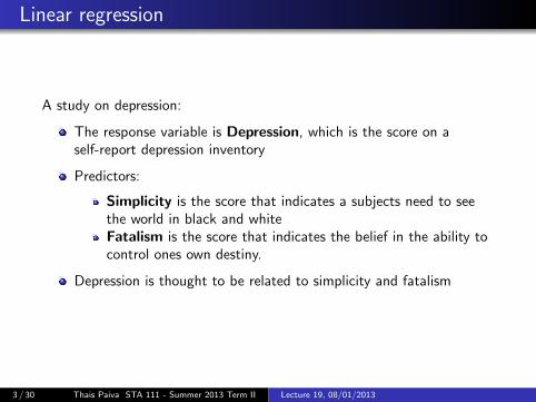
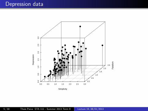
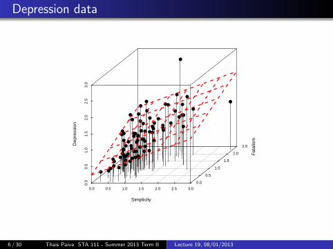
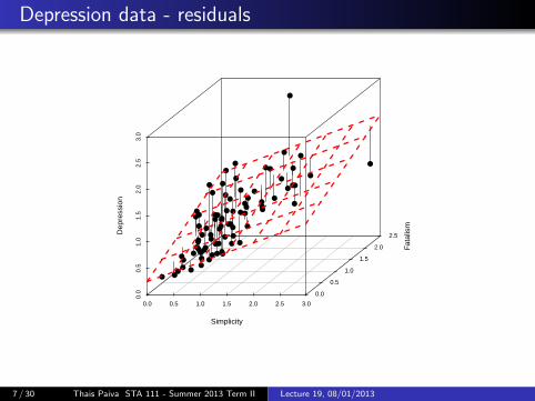
A study on depression:
The response variable is Depression, which is the score on aself-report depression inventory
Predictors:
Simplicity is the score that indicates a subjects need to seethe world in black and whiteFatalism is the score that indicates the belief in the ability tocontrol ones own destiny.
Depression is thought to be related to simplicity and fatalism
3 / 30 Thais Paiva STA 111 - Summer 2013 Term II Lecture 19, 08/01/2013
Linear regression
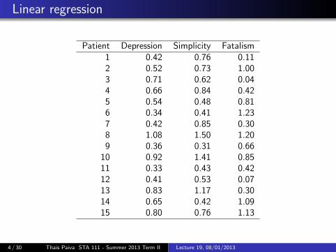
Patient Depression Simplicity Fatalism1 0.42 0.76 0.112 0.52 0.73 1.003 0.71 0.62 0.044 0.66 0.84 0.425 0.54 0.48 0.816 0.34 0.41 1.237 0.42 0.85 0.308 1.08 1.50 1.209 0.36 0.31 0.66
10 0.92 1.41 0.8511 0.33 0.43 0.4212 0.41 0.53 0.0713 0.83 1.17 0.3014 0.65 0.42 1.0915 0.80 0.76 1.13
4 / 30 Thais Paiva STA 111 - Summer 2013 Term II Lecture 19, 08/01/2013
Depression data
0.0 0.5 1.0 1.5 2.0 2.5 3.0
0.0
0.5
1.0
1.5
2.0
2.5
3.0
0.0
0.5
1.0
1.5
2.0
2.5
Simplicity
Fata
lism
Dep
ress
ion
●
●
●
●
●
●
●
●
●●
●
●
●
●
●
●●
●
●
●●
●
●
●
●
●●
●
●
●
●
●
●
●
●
●
●
●●
●
●
●●
●
●
●
●
●
●●
●
●●
●
●●
●
●
●●
●
●
●
●●
●
●
●
●●●
●
●
●
●
●●
●●
●
● ●
5 / 30 Thais Paiva STA 111 - Summer 2013 Term II Lecture 19, 08/01/2013
Depression data
0.0 0.5 1.0 1.5 2.0 2.5 3.0
0.0
0.5
1.0
1.5
2.0
2.5
3.0
0.0
0.5
1.0
1.5
2.0
2.5
Simplicity
Fata
lism
Dep
ress
ion
●
●
●
●
●
●
●
●
●●
●
●
●
●
●
●●
●
●
●●
●
●
●
●
●●
●
●
●
●
●
●
●
●
●
●
●●
●
●
●●
●
●
●
●
●
●●
●
●●
●
●●
●
●
●●
●
●
●
●●
●
●
●
●●●
●
●
●
●
●●
●●
●
● ●
6 / 30 Thais Paiva STA 111 - Summer 2013 Term II Lecture 19, 08/01/2013
Depression data - residuals
0.0 0.5 1.0 1.5 2.0 2.5 3.0
0.0
0.5
1.0
1.5
2.0
2.5
3.0
0.0
0.5
1.0
1.5
2.0
2.5
Simplicity
Fata
lism
Dep
ress
ion
●
●
●
●
●
●
●
●
●●
●
●
●
●
●
●●
●
●
●●
●
●
●
●
●●
●
●
●
●
●
●
●
●
●
●
●●
●
●
●●
●
●
●
●
●
●●
●
●●
●
●●
●
●
●●
●
●
●
●●
●
●
●
●●●
●
●
●
●
●●
●●
●
● ●
7 / 30 Thais Paiva STA 111 - Summer 2013 Term II Lecture 19, 08/01/2013
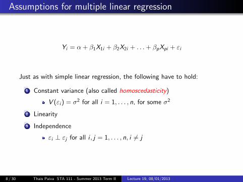
Assumptions for multiple linear regression
Yi = α + β1X1i + β2X2i + . . .+ βpXpi + εi
Just as with simple linear regression, the following have to hold:
1 Constant variance (also called homoscedasticity)
V (εi ) = σ2 for all i = 1, . . . , n, for some σ2
2 Linearity
3 Independence
εi ⊥ εj for all i , j = 1, . . . , n, i 6= j
8 / 30 Thais Paiva STA 111 - Summer 2013 Term II Lecture 19, 08/01/2013
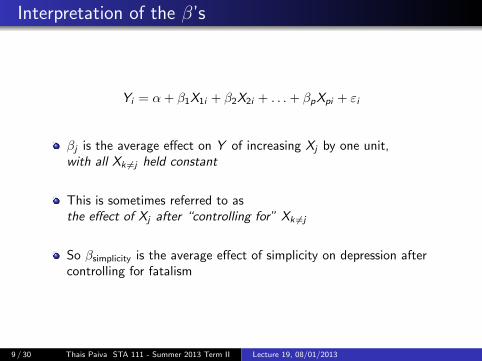
Interpretation of the β’s
Yi = α + β1X1i + β2X2i + . . .+ βpXpi + εi
βj is the average effect on Y of increasing Xj by one unit,with all Xk 6=j held constant
This is sometimes referred to asthe effect of Xj after “controlling for” Xk 6=j
So βsimplicity is the average effect of simplicity on depression aftercontrolling for fatalism
9 / 30 Thais Paiva STA 111 - Summer 2013 Term II Lecture 19, 08/01/2013
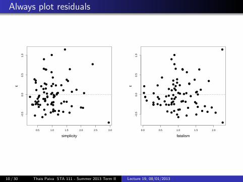
Always plot residuals
●
●
●
●
●
●
●
●
●
●●
●
●
● ●
●
●
●
●
●
●
●
●
●
●
●
●●
●
●
●●
● ●
●
●●
●
●
●
●
●
●
●
●
●
●
●
●
●
●
●
●
●
●●
●
●
●
●
●
●
●
●
●
●
●
●
●
●
●
●
● ●
●
●
●●
●
●
●
●
0.5 1.0 1.5 2.0 2.5 3.0
−0.
50.
00.
51.
0
simplicity
ε
●
●
●
●
●
●
●
●
●
●●
●
●
●●
●
●
●
●
●
●
●
●
●
●
●
●●
●
●
●●
● ●
●
●●
●
●
●
●
●
●
●
●
●
●
●
●
●
●
●
●
●
●●
●
●
●
●
●
●
●
●
●
●
●
●
●
●
●
●
●●
●
●
● ●
●
●
●
●
0.0 0.5 1.0 1.5 2.0
−0.
50.
00.
51.
0fatalism
ε
10 / 30 Thais Paiva STA 111 - Summer 2013 Term II Lecture 19, 08/01/2013
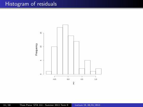
Histogram of residuals
ε
Fre
quen
cy
−0.5 0.0 0.5 1.0
05
1015
11 / 30 Thais Paiva STA 111 - Summer 2013 Term II Lecture 19, 08/01/2013
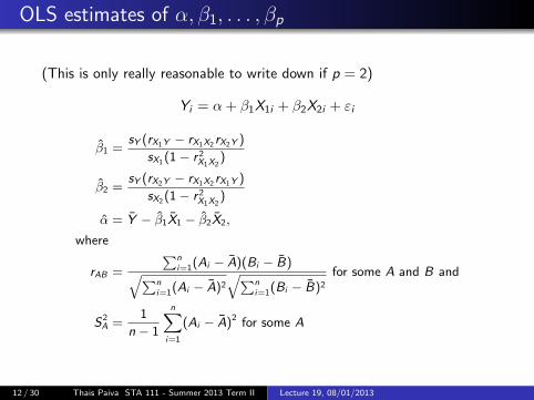
OLS estimates of α, β1, . . . , βp
(This is only really reasonable to write down if p = 2)
Yi = α + β1X1i + β2X2i + εi
β1 =sY (rX1Y − rX1X2 rX2Y )
sX1(1 − r 2X1X2)
β2 =sY (rX2Y − rX1X2 rX1Y )
sX2(1 − r 2X1X2)
α = Y − β1X1 − β2X2,
where
rAB =
∑ni=1(Ai − A)(Bi − B)√∑n
i=1(Ai − A)2√∑n
i=1(Bi − B)2for some A and B and
S2A =
1
n − 1
n∑i=1
(Ai − A)2 for some A
12 / 30 Thais Paiva STA 111 - Summer 2013 Term II Lecture 19, 08/01/2013
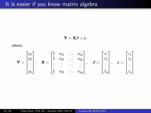
It is easier if you know matrix algebra
Y = Xβ + ε,
where
Y =
y1y2...
yn
, X =
1 x11 . . . x1p1 x21 . . . x2p...
.... . .
...1 x21 . . . xnp
, β =
αβ1...βp
, ε =
ε1ε2...εn
13 / 30 Thais Paiva STA 111 - Summer 2013 Term II Lecture 19, 08/01/2013
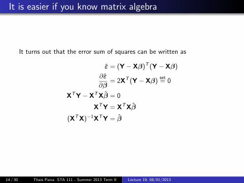
It is easier if you know matrix algebra
It turns out that the error sum of squares can be written as
ε = (Y − Xβ)T (Y − Xβ)
∂ε
∂β= 2XT (Y − Xβ)
set= 0
XTY − XTXβ = 0
XTY = XTXβ
(XTX)−1XTY = β
14 / 30 Thais Paiva STA 111 - Summer 2013 Term II Lecture 19, 08/01/2013

It is easier if you know matrix algebra
A couple of things are clear
β = (XTX)−1XTY
1 β is linear in Y
2 β is easy to compute if we have a computer
15 / 30 Thais Paiva STA 111 - Summer 2013 Term II Lecture 19, 08/01/2013
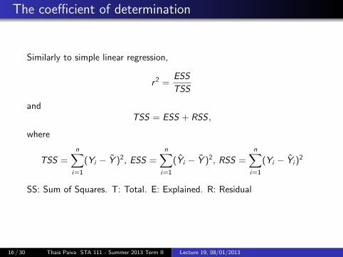
The coefficient of determination
Similarly to simple linear regression,
r2 =ESS
TSS
andTSS = ESS + RSS ,
where
TSS =n∑
i=1
(Yi − Y )2, ESS =n∑
i=1
(Yi − Y )2, RSS =n∑
i=1
(Yi − Yi )2
SS: Sum of Squares. T: Total. E: Explained. R: Residual
16 / 30 Thais Paiva STA 111 - Summer 2013 Term II Lecture 19, 08/01/2013
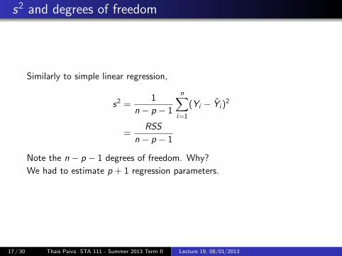
s2 and degrees of freedom
Similarly to simple linear regression,
s2 =1
n − p − 1
n∑i=1
(Yi − Yi )2
=RSS
n − p − 1
Note the n − p − 1 degrees of freedom. Why?
We had to estimate p + 1 regression parameters.
17 / 30 Thais Paiva STA 111 - Summer 2013 Term II Lecture 19, 08/01/2013
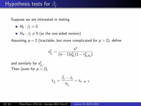
Hypothesis tests for βj
Suppose we are interested in testing
H0 : βj = 0
HA : βj 6= 0 (or the one-sided version)
Assuming p = 2 (tractable, but more complicated for p > 2), define
s2β1
=s2
(n − 1)s2X1(1− r2X1X2
)
and similarly for s2β2
.
Then (even for p > 2),
tβj=βj − βj
sβj
∼ tn−p−1
18 / 30 Thais Paiva STA 111 - Summer 2013 Term II Lecture 19, 08/01/2013
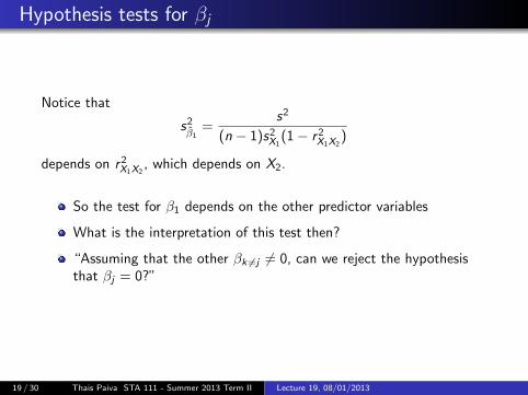
Hypothesis tests for βj
Notice that
s2β1
=s2
(n − 1)s2X1(1− r2X1X2
)
depends on r2X1X2, which depends on X2.
So the test for β1 depends on the other predictor variables
What is the interpretation of this test then?
“Assuming that the other βk 6=j 6= 0, can we reject the hypothesisthat βj = 0?”
19 / 30 Thais Paiva STA 111 - Summer 2013 Term II Lecture 19, 08/01/2013

Scatterplot matrix
●
depression
0.5 1.0 1.5 2.0 2.5 3.0
●●
●●
●
●●
●
●
●
●●
●
●
●
●●●
●● ●
● ●
●
●
●
●●
●
●
●●
●
●●
●
● ●
●
●●
●
●
●●
●
●
●
●
●●●
●
●
●●●
●
●●●
●
●
● ●
●
●
●●●
●
●
●●
●●
●
● ●
●
●
●
0.5
1.0
1.5
2.0
2.5
●●
●●
●
●●
●
●
●
●●
●
●
●
●●●
●● ●
●●
●
●
●
●●
●
●
●●
●
●●
●
●●
●
●●
●
●
●●
●
●
●
●
●●●
●
●
●●●
●
●●●
●
●
● ●
●
●
● ●●
●
●
●●
●●
●
● ●
●
●
●
0.5
1.0
1.5
2.0
2.5
3.0
● ●●
●
●●
●
●
●
●
●●
●
●
●
●
●
●
●●
●
●
●
●
●●
●
●
●●
●
●
●
●●
●●
●
●
●
●
● ●
●
●
●
●
●
●
●
●●
●
●
●●
●
●
●●
●
●
●●
●
●
●
●●
●
●●
●
●
●
●
●
●
●
●
●
●
●
●
●
●
●
simplicity
● ●●
●
●●
●
●
●
●
●●
●
●
●
●
●
●
●●
●
●
●
●
●●
●
●
●●
●
●
●
● ●
●●
●
●
●
●
● ●
●
●
●
●
●
●
●
●●
●
●
●●
●
●
●●
●
●
● ●
●
●
●
●●
●
●●
●
●
●
●
●
●
●
●
●
●
0.5 1.0 1.5 2.0 2.5
●
●
●
●
●
●
●
●
●
●
●
●
●
● ●
●
●
●
●●
●
●
●
●
●
●
●
●
●
●
●
●
●
●
●
●
●
●
● ●
●
●
●
●●
●
●
●
●
●
●●
●
●
●
●
●●
●
●
●
●
●
●
●
●
●
●
●
●
●
●
● ●
●
●
●
●
●
●
●
●
●
●
●
●
●
●
●
●
●
●
●
●
●
● ●
●
●
●
●●
●
●
●
●
●
●
●
●
●
●
●
●
●
●
●
●
●
●
● ●
●
●
●
●●
●
●
●
●
●
●●
●
●
●
●
● ●
●
●
●
●
●
●
●
●
●
●
●
●
●
●
● ●
●
●
●
●
●
●
●
●
0.0 0.5 1.0 1.5 2.0
0.0
0.5
1.0
1.5
2.0
●●
fatalism
20 / 30 Thais Paiva STA 111 - Summer 2013 Term II Lecture 19, 08/01/2013
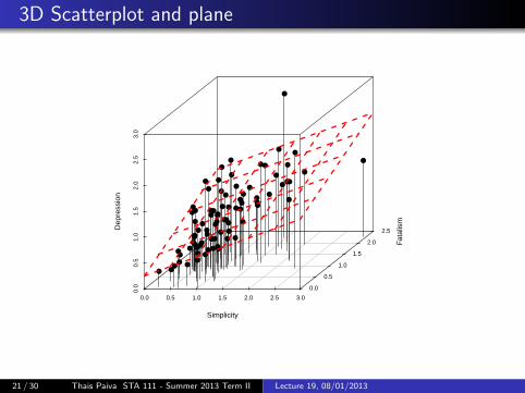
3D Scatterplot and plane
0.0 0.5 1.0 1.5 2.0 2.5 3.0
0.0
0.5
1.0
1.5
2.0
2.5
3.0
0.0
0.5
1.0
1.5
2.0
2.5
Simplicity
Fata
lism
Dep
ress
ion
●
●
●
●
●
●
●
●
●●
●
●
●
●
●
●●
●
●
●●
●
●
●
●
●●
●
●
●
●
●
●
●
●
●
●
●●
●
●
●●
●
●
●
●
●
●●
●
●●
●
●●
●
●
●●
●
●
●
●●
●
●
●
●●●
●
●
●
●
●●
●●
●
● ●
21 / 30 Thais Paiva STA 111 - Summer 2013 Term II Lecture 19, 08/01/2013
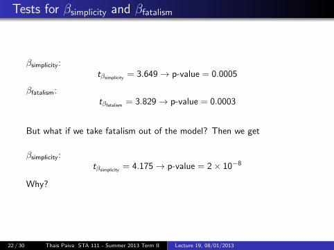
Tests for βsimplicity and βfatalism
βsimplicity:tβsimplicity
= 3.649→ p-value = 0.0005
βfatalism:tβfatalism
= 3.829→ p-value = 0.0003
But what if we take fatalism out of the model? Then we get
βsimplicity:tβsimplicity
= 4.175→ p-value = 2× 10⁻⁸
Why?
22 / 30 Thais Paiva STA 111 - Summer 2013 Term II Lecture 19, 08/01/2013
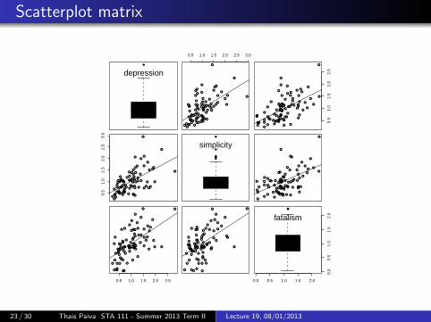
Scatterplot matrix
●
depression
0.5 1.0 1.5 2.0 2.5 3.0
●●
●●
●
●●
●
●
●
●●
●
●
●
●●●
●● ●
● ●
●
●
●
●●
●
●
●●
●
●●
●
● ●
●
●●
●
●
●●
●
●
●
●
●●●
●
●
●●●
●
●●●
●
●
● ●
●
●
●●●
●
●
●●
●●
●
● ●
●
●
●
0.5
1.0
1.5
2.0
2.5
●●
●●
●
●●
●
●
●
●●
●
●
●
●●●
●● ●
●●
●
●
●
●●
●
●
●●
●
●●
●
●●
●
●●
●
●
●●
●
●
●
●
●●●
●
●
●●●
●
●●●
●
●
● ●
●
●
● ●●
●
●
●●
●●
●
● ●
●
●
●
0.5
1.0
1.5
2.0
2.5
3.0
● ●●
●
●●
●
●
●
●
●●
●
●
●
●
●
●
●●
●
●
●
●
●●
●
●
●●
●
●
●
●●
●●
●
●
●
●
● ●
●
●
●
●
●
●
●
●●
●
●
●●
●
●
●●
●
●
●●
●
●
●
●●
●
●●
●
●
●
●
●
●
●
●
●
●
●
●
●
●
●
simplicity
● ●●
●
●●
●
●
●
●
●●
●
●
●
●
●
●
●●
●
●
●
●
●●
●
●
●●
●
●
●
● ●
●●
●
●
●
●
● ●
●
●
●
●
●
●
●
●●
●
●
●●
●
●
●●
●
●
● ●
●
●
●
●●
●
●●
●
●
●
●
●
●
●
●
●
●
0.5 1.0 1.5 2.0 2.5
●
●
●
●
●
●
●
●
●
●
●
●
●
● ●
●
●
●
●●
●
●
●
●
●
●
●
●
●
●
●
●
●
●
●
●
●
●
● ●
●
●
●
●●
●
●
●
●
●
●●
●
●
●
●
●●
●
●
●
●
●
●
●
●
●
●
●
●
●
●
● ●
●
●
●
●
●
●
●
●
●
●
●
●
●
●
●
●
●
●
●
●
●
● ●
●
●
●
●●
●
●
●
●
●
●
●
●
●
●
●
●
●
●
●
●
●
●
● ●
●
●
●
●●
●
●
●
●
●
●●
●
●
●
●
● ●
●
●
●
●
●
●
●
●
●
●
●
●
●
●
● ●
●
●
●
●
●
●
●
●
0.0 0.5 1.0 1.5 2.0
0.0
0.5
1.0
1.5
2.0
●●
fatalism
23 / 30 Thais Paiva STA 111 - Summer 2013 Term II Lecture 19, 08/01/2013

1907 Romanian Peasant Rebellion
From Wikipedia:
The Romanian Peasants’ Revolt took place in March 1907 in Moldaviaand it quickly spread, reaching Wallachia.
Y = Intensity of the rebellion, by county
X1 = Commercialization of agriculture
X2 = Traditionalism
X3 = Strength of middle peasantry
X4 = Inequality of land tenure
24 / 30 Thais Paiva STA 111 - Summer 2013 Term II Lecture 19, 08/01/2013
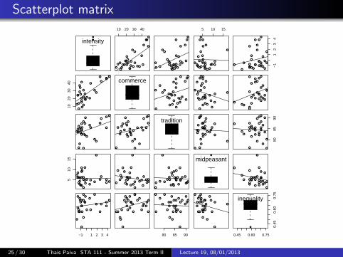
Scatterplot matrix
●
●●intensity
10 20 30 40
●
●
●
●
●
●
●●
●
●
●
●
●
●
●
●● ●●
●
●
●
●
●
●●
●
●
●
●
●
●
●
●
●
●
●●
●
●
●
●
●
●
●
●●●●
●
●
●
●
●
●●
●
●
●
●
5 10 15
●
●
●
●
●
●
●●
●
●
●
●
●
●
●
●● ●●
●
●
●
●
●
● ●
●
●
●
● −1
12
34
●
●
●
●
●
●
●●
●
●
●
●
●
●
●
●● ●●
●
●
●
●
●
●●
●
●
●
●
1020
3040
●
●
●
●●
●
●
● ●
●
●●
●●
●●
●
●
●
●
●
●
●
●●●
●
●
●
●
commerce
●
●
●
●●
●
●
● ●
●
●●
●●
●●
●
●
●
●
●
●
●
●●●
●
●
●
●●
●
●
●●
●
●
●●
●
●●
●●
●●
●
●
●
●
●
●
●
●● ●
●
●
●
●●
●
●
●●
●
●
● ●
●
●●
●●
●●
●
●
●
●
●
●
●
●●●
●
●
●
●
● ●
●
●
●
●●●
●
●
●
●
●
●
●
●
●
●
●
●
●
●
●
●●
●
●
●
●●● ●
●
●
●
●● ●
●
●
●
●
●
●
●
●
●
●
●
●
●
●
●
●●
●
●
●
●●tradition
●●
●
●
●
●● ●
●
●
●
●
●
●
●
●
●
●
●
●
●
●
●
●●
●
●
●
● ●
8085
90
● ●
●
●
●
●● ●
●
●
●
●
●
●
●
●
●
●
●
●
●
●
●
●●
●
●
●
●●
510
15
●
●
●
●
●
●●●
●
●
●
●
●●
●
●
●
●
●●
●
●
● ●●
●
●
● ●
●
●
●
●
●
●
●●●
●
●
●
●
●●
●
●
●
●
●●
●
●
● ●●
●
●
● ●
●
●
●
●
●
●
● ●●
●
●
●
●
●●
●
●
●
●
●●
●
●
● ●●
●
●
● ●
●
●
midpeasant
●
●
●
●
●
●●●
●
●
●
●
●●
●
●
●
●
●●
●
●
●●●
●
●
●●
●
−1 1 2 3 4
●
●
●
●
●
●
●
●
●
●
●
●
●
●
●
●
●
●
●
●
●●
●
●●
●
●
●●
●
●
●
●
●
●
●
●
●
●
●
●
●
●
●
●
●
●
●
●
●
●●
●
●●
●
●
●●
●
80 85 90
●
●
●
●
●
●
●
●
●
●
●
●
●
●
●
●
●
●
●
●
●●
●
●●
●
●
●●
●
●
●
●
●
●
●
●
●
●
●
●
●
●
●
●
●
●
●
●
●
●●
●
●●
●
●
●●
●
0.45 0.60 0.75
0.45
0.60
0.75
●
inequality
25 / 30 Thais Paiva STA 111 - Summer 2013 Term II Lecture 19, 08/01/2013
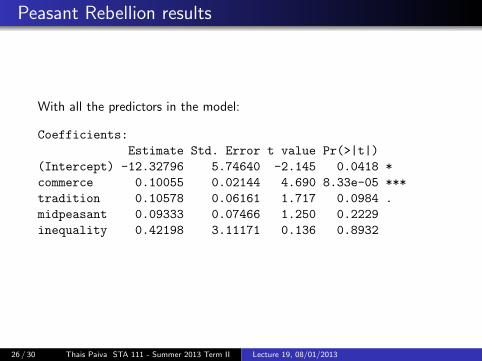
Peasant Rebellion results
With all the predictors in the model:
Coefficients:
Estimate Std. Error t value Pr(>|t|)
(Intercept) -12.32796 5.74640 -2.145 0.0418 *
commerce 0.10055 0.02144 4.690 8.33e-05 ***
tradition 0.10578 0.06161 1.717 0.0984 .
midpeasant 0.09333 0.07466 1.250 0.2229
inequality 0.42198 3.11171 0.136 0.8932
26 / 30 Thais Paiva STA 111 - Summer 2013 Term II Lecture 19, 08/01/2013
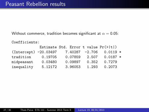
Peasant Rebellion results
Without commerce, tradition becomes significant at α = 0.05:
Coefficients:
Estimate Std. Error t value Pr(>|t|)
(Intercept) -20.03497 7.40287 -2.706 0.0119 *
tradition 0.19705 0.07859 2.507 0.0187 *
midpeasant 0.03480 0.09897 0.352 0.7279
inequality 5.12172 3.96053 1.293 0.2073
27 / 30 Thais Paiva STA 111 - Summer 2013 Term II Lecture 19, 08/01/2013
Caveats
1 Be careful interpreting the coefficients! Multiple regression is usuallyapplied to observational data
2 Do not think of the sign of the coefficient as special – it can actuallychange as other covariates are added or removed from the model
3 Similarly, tests about any covariate are only meaningful in thecontext of the other covariates in the model
4 Always make sure a linear model is appropriate for all predictors!
5 Always check residuals for heteroscedasticity and normality
28 / 30 Thais Paiva STA 111 - Summer 2013 Term II Lecture 19, 08/01/2013
Caveats
In particular, a special case that you should be careful about is whenthe predictors are highly correlated
In this situation the coefficient estimates may change erratically inresponse to small changes in the model or the data
This phenomenon is called multicollinearity
Because of that, matrix correlation of the predictors is alsosomething to look at (and report) in the analysis
29 / 30 Thais Paiva STA 111 - Summer 2013 Term II Lecture 19, 08/01/2013
Summary
1 Multiple linear regression fits the best hyperplane to the data
2 We can test hypotheses about any of the βj ’s
3 Be careful about interpretation
4 Correlation of the predictors also important because ofmulticollinearity
30 / 30 Thais Paiva STA 111 - Summer 2013 Term II Lecture 19, 08/01/2013