Introduction to Big Bang Cosmology

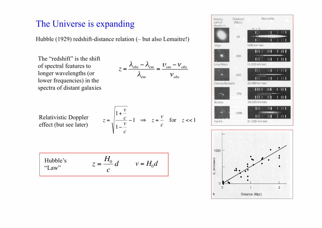
The Universe is expanding Hubble (1929) redshift-distance relation (– but also Lemaitre!)

z = λobs −λemλem

=υem −νobs

νobs

z Hcd= 0

z

vcvc

z vc

z=+

−− ⇒ = <<

1

11 1for

v H d= 0

The “redshift” is the shift of spectral features to longer wavelengths (or lower frequencies) in the spectra of distant galaxies

Relativistic Doppler effect (but see later)

Hubble’s “Law”

5 lo

g (d

ista

nce)

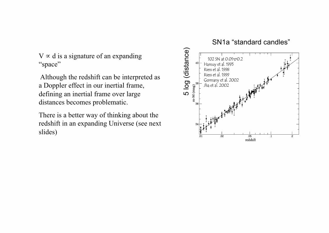
SN1a “standard candles”

V ∝ d is a signature of an expanding “space”

Although the redshift can be interpreted as a Doppler effect in our inertial frame, defining an inertial frame over large distances becomes problematic.

There is a better way of thinking about the redshift in an expanding Universe (see next slides)

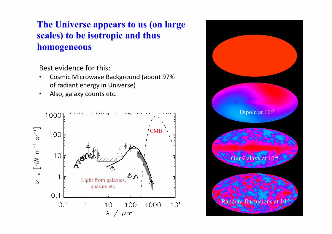
The Universe appears to us (on large scales) to be isotropic and thus homogeneous

Bestevidenceforthis:•  CosmicMicrowaveBackground(about97%

ofradiantenergyinUniverse)•  Also,galaxycountsetc.

Dipole at 10-3

Our Galaxy at 10-4

Random fluctuaions at 10-5

CMB

Light from galaxies, quasars etc.

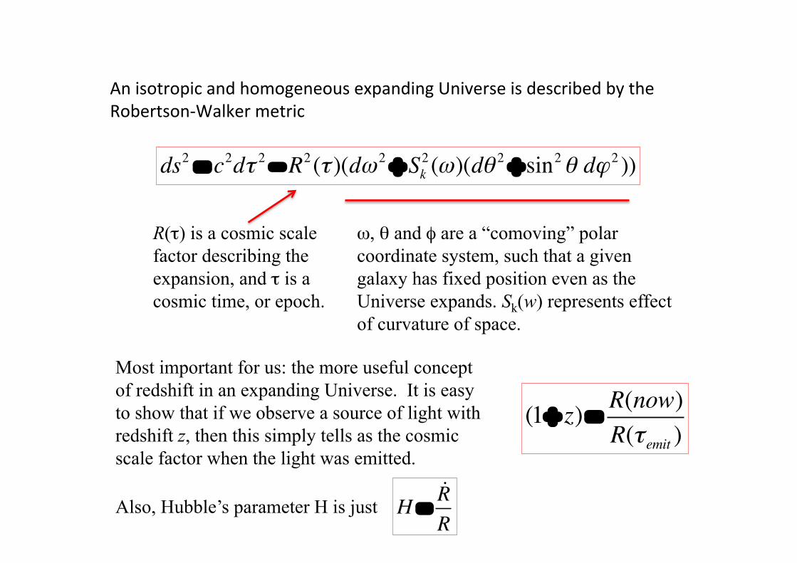
AnisotropicandhomogeneousexpandingUniverseisdescribedbytheRobertson-Walkermetric

ds2 = c2dτ 2 − R2 (τ )(dω 2 + Sk2 (ω)(dθ 2 + sin2θ dϕ 2 ))

ω, θ and φ are a “comoving” polar coordinate system, such that a given galaxy has fixed position even as the Universe expands. Sk(w) represents effect of curvature of space.

R(τ) is a cosmic scale factor describing the expansion, and τ is a cosmic time, or epoch.

Most important for us: the more useful concept of redshift in an expanding Universe. It is easy to show that if we observe a source of light with redshift z, then this simply tells as the cosmic scale factor when the light was emitted.

(1+ z) = R(now)R(τ emit )

Also, Hubble’s parameter H is just H =!RR

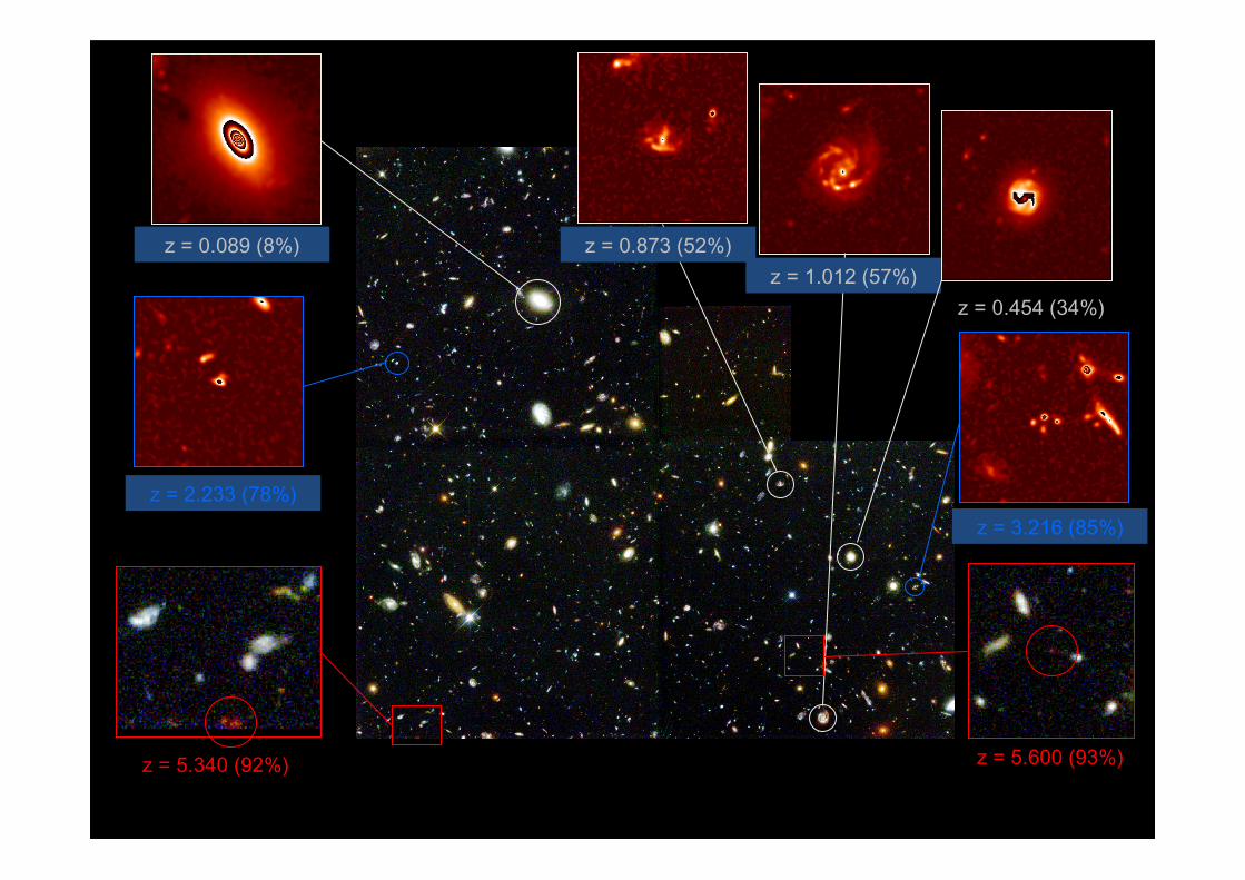
Hubble Deep Field and redshifts

z = 5.340 (92%) z = 5.600 (93%)

z = 1.012 (57%) z = 0.454 (34%)

z = 3.216 (85%)

z = 0.089 (8%)

z = 2.233 (78%)

z = 0.873 (52%)

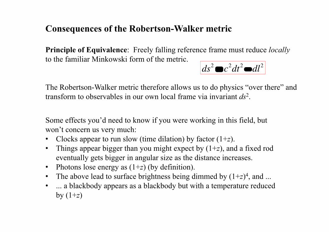
Consequences of the Robertson-Walker metric Principle of Equivalence: Freely falling reference frame must reduce locally to the familiar Minkowski form of the metric. The Robertson-Walker metric therefore allows us to do physics “over there” and transform to observables in our own local frame via invariant ds2.

Some effects you’d need to know if you were working in this field, but won’t concern us very much: •  Clocks appear to run slow (time dilation) by factor (1+z). •  Things appear bigger than you might expect by (1+z), and a fixed rod

eventually gets bigger in angular size as the distance increases. •  Photons lose energy as (1+z) (by definition). •  The above lead to surface brightness being dimmed by (1+z)4, and ... •  ... a blackbody appears as a blackbody but with a temperature reduced

by (1+z)

ds2 = c2dt2 − dl2

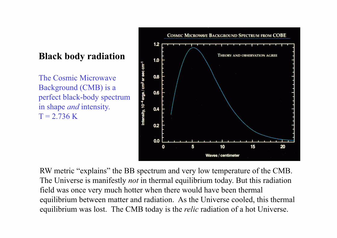
Black body radiation The Cosmic Microwave Background (CMB) is a perfect black-body spectrum in shape and intensity. T = 2.736 K

RW metric “explains” the BB spectrum and very low temperature of the CMB. The Universe is manifestly not in thermal equilibrium today. But this radiation field was once very much hotter when there would have been thermal equilibrium between matter and radiation. As the Universe cooled, this thermal equilibrium was lost. The CMB today is the relic radiation of a hot Universe.

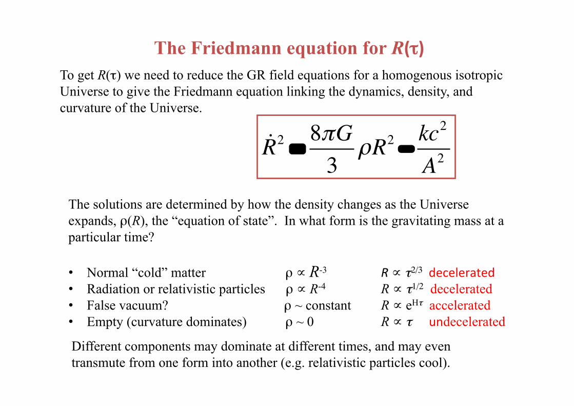
The Friedmann equation for R(τ)To get R(τ) we need to reduce the GR field equations for a homogenous isotropic Universe to give the Friedmann equation linking the dynamics, density, and curvature of the Universe.

!R2 = 8πG3

ρR2 − kc2

A2

The solutions are determined by how the density changes as the Universe expands, ρ(R), the “equation of state”. In what form is the gravitating mass at a particular time? •  Normal “cold” matter ρ ∝ R-3 •  Radiation or relativistic particles ρ ∝ R-4 •  False vacuum? ρ ~ constant •  Empty (curvature dominates) ρ ~ 0

Different components may dominate at different times, and may even transmute from one form into another (e.g. relativistic particles cool).

R ∝ τ2/3deceleratedR ∝ τ1/2 decelerated R ∝ eHτ accelerated

R ∝ τ undecelerated

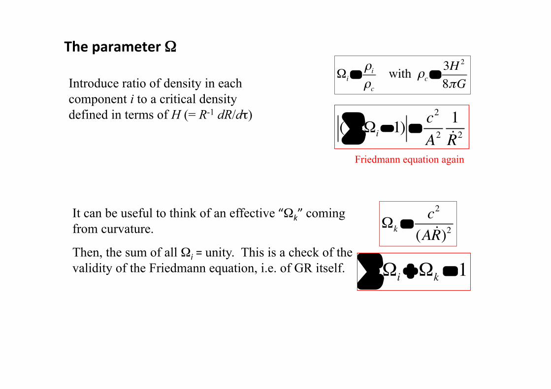
TheparameterΩ

( Ωi∑ −1) = c2

A21!R2

It can be useful to think of an effective“Ωk”coming from curvature.

Then, the sum of all Ωi=unity. This is a check of the validity of the Friedmann equation, i.e. of GR itself.

Ωk =c2

(A !R)2

Ωi =ρiρc

with ρc =3H 2

8πGIntroduce ratio of density in each component i to a critical density defined in terms of H (= R-1 dR/dτ)

Friedmann equation again

Ωi∑ +Ωk =1

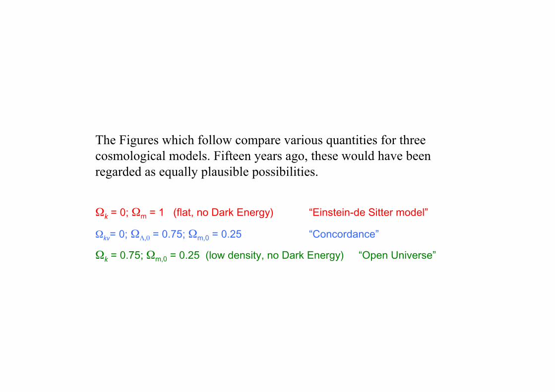
The Figures which follow compare various quantities for three cosmological models. Fifteen years ago, these would have been regarded as equally plausible possibilities.

Ωk= 0; Ωm = 1 (flat, no Dark Energy) “Einstein-de Sitter model”

Ωkv= 0; ΩΛ,0 = 0.75; Ωm,0 = 0.25 “Concordance”

Ωk= 0.75; Ωm,0 = 0.25 (low density, no Dark Energy) “Open Universe”

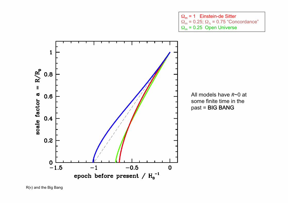
R(τ) and the Big Bang

Ωm = 1 Einstein-de Sitter Ωm = 0.25; ΩΛ = 0.75 “Concordance” Ωm = 0.25 Open Universe

All models have R~0 at some finite time in the past = BIG BANG

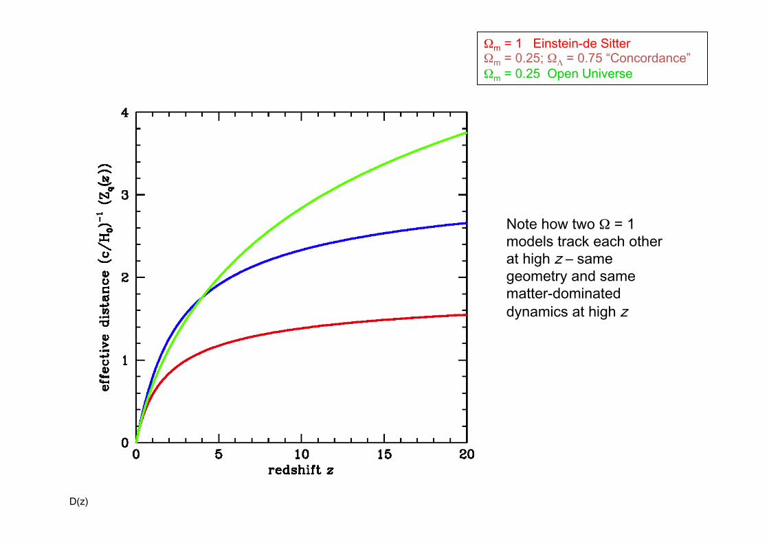
D(z)

Ωm = 1 Einstein-de Sitter Ωm = 0.25; ΩΛ = 0.75 “Concordance” Ωm = 0.25 Open Universe

Note how two Ω = 1 models track each other at high z – same geometry and same matter-dominated dynamics at high z

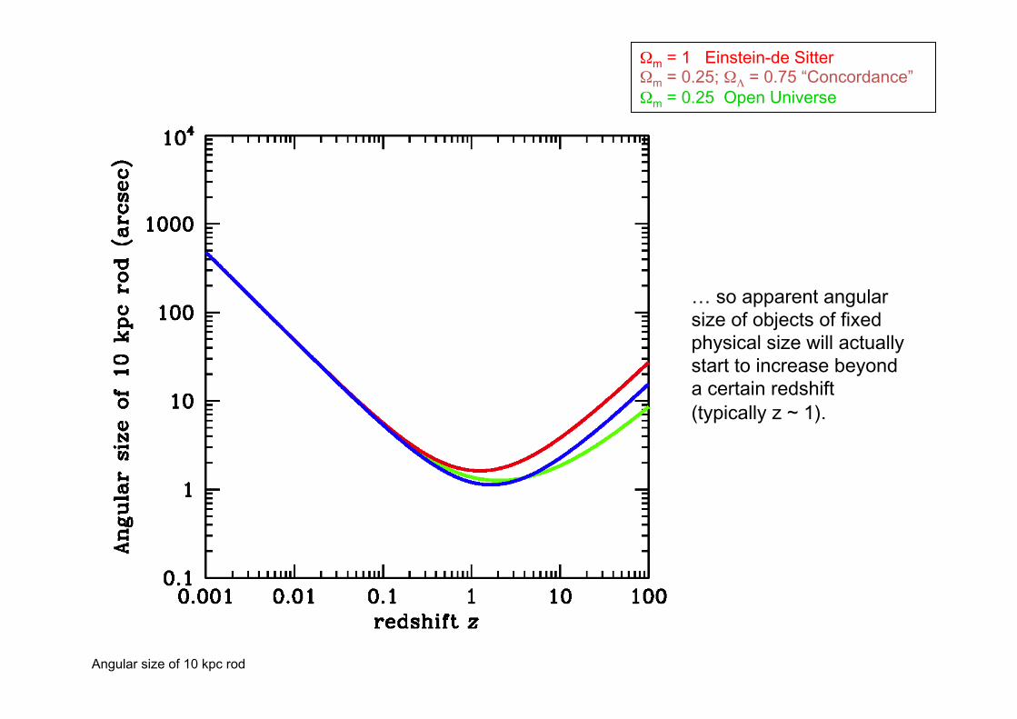
Angular size of 10 kpc rod

Ωm = 1 Einstein-de Sitter Ωm = 0.25; ΩΛ = 0.75 “Concordance” Ωm = 0.25 Open Universe

… so apparent angular size of objects of fixed physical size will actually start to increase beyond a certain redshift (typically z ~ 1).

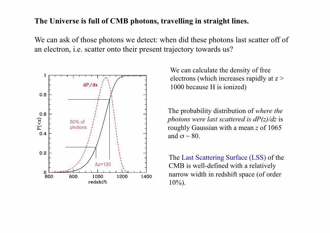
50% of photons

Δz=120

The Universe is full of CMB photons, travelling in straight lines. We can ask of those photons we detect: when did these photons last scatter off of an electron, i.e. scatter onto their present trajectory towards us?

The probability distribution of where the photons were last scattered is dP(z)/dz is roughly Gaussian with a mean z of 1065 and σ ~ 80.

The Last Scattering Surface (LSS) of the CMB is well-defined with a relatively narrow width in redshift space (of order 10%).

We can calculate the density of free electrons (which increases rapidly at z > 1000 because H is ionized)

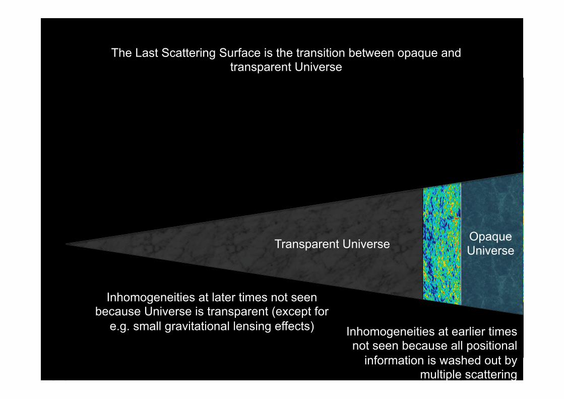
Transparent Universe Opaque Universe

The Last Scattering Surface is the transition between opaque and transparent Universe

Inhomogeneities at later times not seen because Universe is transparent (except for

e.g. small gravitational lensing effects) Inhomogeneities at earlier times not seen because all positional

information is washed out by multiple scattering

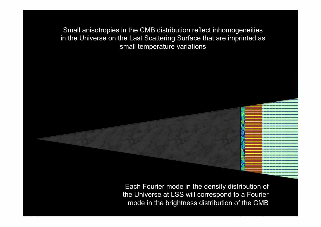
Small anisotropies in the CMB distribution reflect inhomogeneities in the Universe on the Last Scattering Surface that are imprinted as

small temperature variations

Each Fourier mode in the density distribution of the Universe at LSS will correspond to a Fourier

mode in the brightness distribution of the CMB

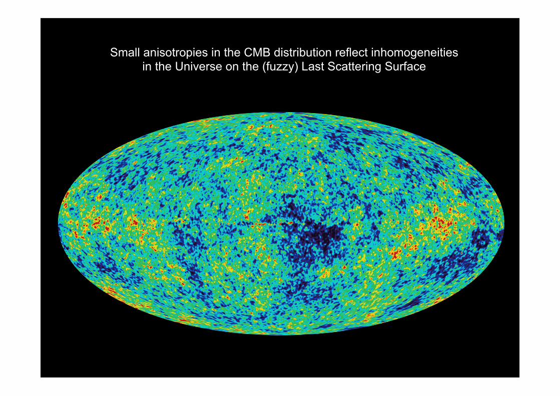
Small anisotropies in the CMB distribution reflect inhomogeneities in the Universe on the (fuzzy) Last Scattering Surface

ΔTT

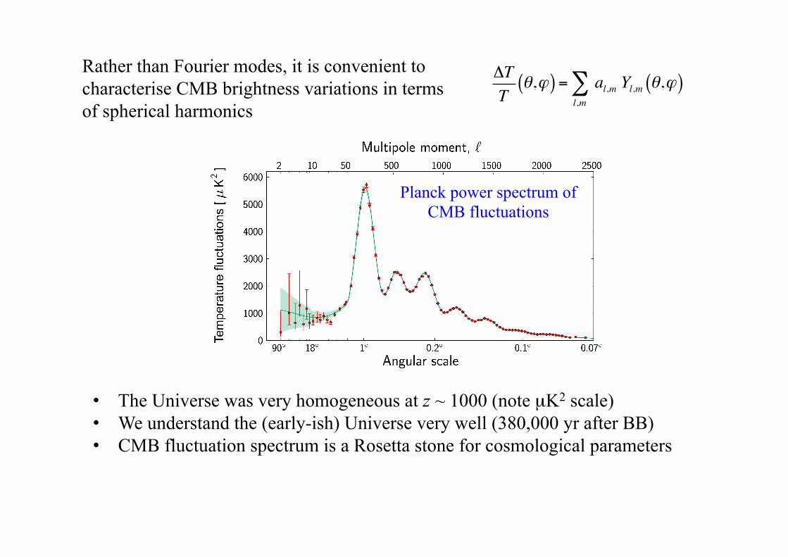
θ,ϕ( ) = al,ml,m∑ Yl,m θ,ϕ( )

Rather than Fourier modes, it is convenient to characterise CMB brightness variations in terms of spherical harmonics

Planck power spectrum of CMB fluctuations

•  The Universe was very homogeneous at z ~ 1000 (note µK2 scale) •  We understand the (early-ish) Universe very well (380,000 yr after BB) •  CMB fluctuation spectrum is a Rosetta stone for cosmological parameters

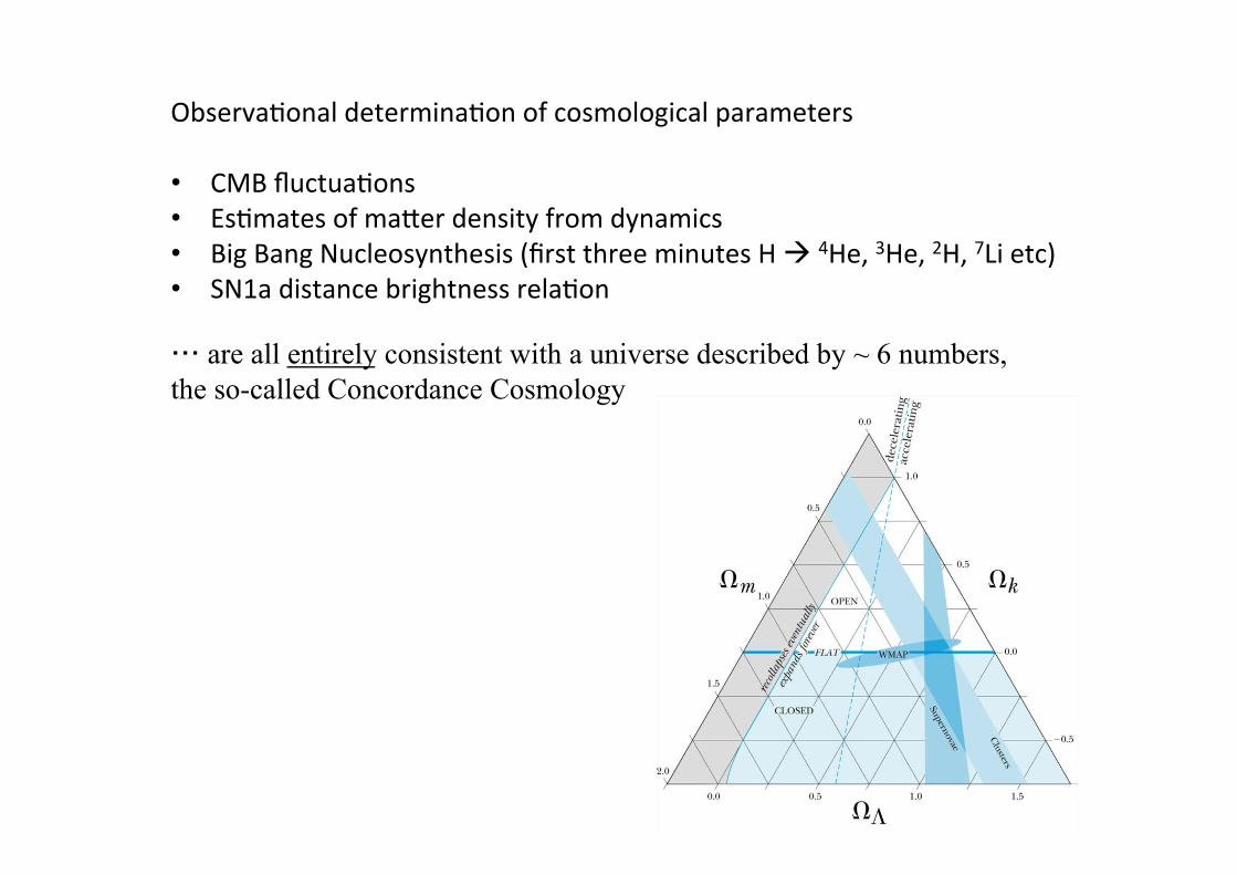
Observational determination of parameters

ObservaMonaldeterminaMonofcosmologicalparameters•  CMBfluctuaMons•  EsMmatesofmaPerdensityfromdynamics•  BigBangNucleosynthesis(firstthreeminutesHà4He,3He,2H,7Lietc)•  SN1adistancebrightnessrelaMon

… are all entirely consistent with a universe described by ~ 6 numbers, the so-called Concordance Cosmology

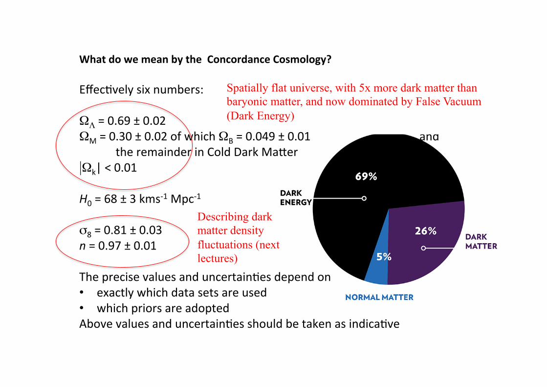
WhatdowemeanbytheConcordanceCosmology?EffecMvelysixnumbers:ΩΛ=0.69±0.02ΩM=0.30±0.02ofwhichΩB=0.049±0.01and

theremainderinColdDarkMaPer|Ωk|<0.01H0=68±3kms-1Mpc-1σ8=0.81±0.03n=0.97±0.01TheprecisevaluesanduncertainMesdependon•  exactlywhichdatasetsareused•  whichpriorsareadoptedAbovevaluesanduncertainMesshouldbetakenasindicaMve

Describing dark matter density fluctuations (next lectures)

Spatially flat universe, with 5x more dark matter than baryonic matter, and now dominated by False Vacuum (Dark Energy)