ELEMENTS OF PROBABILITY THEORY

Elements of Probability Theory

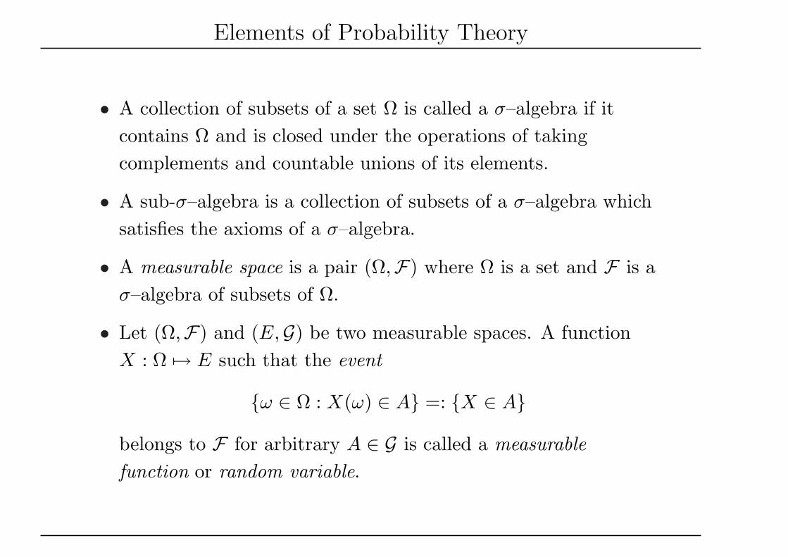
• A collection of subsets of a set Ω is called a σ–algebra if itcontains Ω and is closed under the operations of takingcomplements and countable unions of its elements.

• A sub-σ–algebra is a collection of subsets of a σ–algebra whichsatisfies the axioms of a σ–algebra.

• A measurable space is a pair (Ω,F) where Ω is a set and F is aσ–algebra of subsets of Ω.

• Let (Ω,F) and (E,G) be two measurable spaces. A functionX : Ω 7→ E such that the event

ω ∈ Ω : X(ω) ∈ A =: X ∈ A

belongs to F for arbitrary A ∈ G is called a measurablefunction or random variable.

Elements of Probability Theory

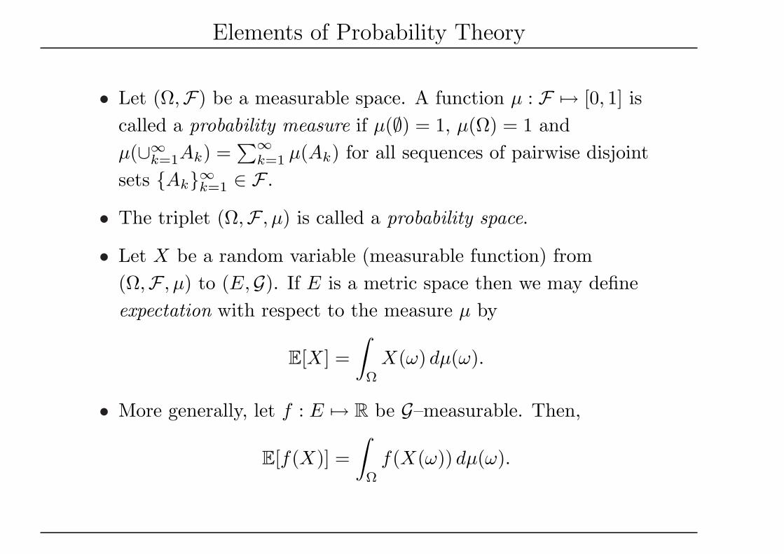
• Let (Ω,F) be a measurable space. A function µ : F 7→ [0, 1] iscalled a probability measure if µ(∅) = 1, µ(Ω) = 1 andµ(∪∞k=1Ak) =

∑∞k=1 µ(Ak) for all sequences of pairwise disjoint

sets Ak∞k=1 ∈ F .

• The triplet (Ω,F , µ) is called a probability space.

• Let X be a random variable (measurable function) from(Ω,F , µ) to (E,G). If E is a metric space then we may defineexpectation with respect to the measure µ by

E[X] =∫

Ω

X(ω) dµ(ω).

• More generally, let f : E 7→ R be G–measurable. Then,

E[f(X)] =∫

Ω

f(X(ω)) dµ(ω).

Elements of Probability Theory

• Let U be a topological space. We will use the notation B(U) todenote the Borel σ–algebra of U : the smallest σ–algebracontaining all open sets of U . Every random variable from aprobability space (Ω,F , µ) to a measurable space (E,B(E))induces a probability measure on E:

µX(B) = PX−1(B) = µ(ω ∈ Ω; X(ω) ∈ B), B ∈ B(E).

The measure µX is called the distribution (or sometimes thelaw) of X.

Example 1 Let I denote a subset of the positive integers. Avector ρ0 = ρ0,i, i ∈ I is a distribution on I if it has nonnegativeentries and its total mass equals 1:

∑i∈I ρ0,i = 1.

Elements of Probability Theory

• We can use the distribution of a random variable to computeexpectations and probabilities:

E[f(X)] =∫

S

f(x) dµX(x)

and

P[X ∈ G] =∫

G

dµX(x), G ∈ B(E).

• When E = Rd and we can write dµX(x) = ρ(x) dx, then werefer to ρ(x) as the probability density function (pdf), ordensity with respect to Lebesque measure for X.

• When E = Rd then by Lp(Ω;Rd), or sometimes Lp(Ω; µ) oreven simply Lp(µ), we mean the Banach space of measurablefunctions on Ω with norm

‖X‖Lp =(E|X|p

)1/p

.

Elements of Probability Theory

Example 2 i) Consider the random variable X : Ω 7→ R with pdf

γσ,m(x) := (2πσ)−12 exp

(− (x−m)2

2σ

).

Such an X is termed a Gaussian or normal random variable.The mean is

EX =∫

Rxγσ,m(x) dx = m

and the variance is

E(X −m)2 =∫

R(x−m)2γσ,m(x) dx = σ.

Since the mean and variance specify completely a Gaussianrandom variable on R, the Gaussian is commonly denoted byN (m,σ). The standard normal random variable is N (0, 1).

Elements of Probability Theory

ii) Let m ∈ Rd and Σ ∈ Rd×d be symmetric and positive definite.The random variable X : Ω 7→ Rd with pdf

γΣ,m(x) :=((2π)ddetΣ

)− 12 exp

(−1

2〈Σ−1(x−m), (x−m)〉

)

is termed a multivariate Gaussian or normal randomvariable. The mean is

E(X) = m (1)

and the covariance matrix is

E((X −m)⊗ (X −m)

)= Σ. (2)

Since the mean and covariance matrix completely specify aGaussian random variable on Rd, the Gaussian is commonlydenoted by N (m,Σ).

Elements of Probability Theory

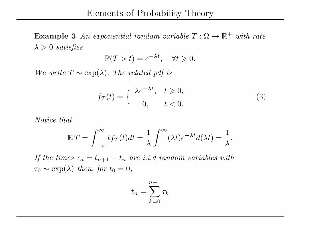
Example 3 An exponential random variable T : Ω → R+ with rateλ > 0 satisfies

P(T > t) = e−λt, ∀t > 0.

We write T ∼ exp(λ). The related pdf is

fT (t) = λe−λt, t > 0,

0, t < 0.(3)

Notice that

ET =∫ ∞

−∞tfT (t)dt =

1λ

∫ ∞

0

(λt)e−λtd(λt) =1λ

.

If the times τn = tn+1 − tn are i.i.d random variables withτ0 ∼ exp(λ) then, for t0 = 0,

tn =n−1∑

k=0

τk

Elements of Probability Theory

and it is possible to show that

P(0 6 tk 6 t < tk+1) =e−λt(λt)k

k!. (4)

Elements of Probability Theory

• Assume that E|X| < ∞ and let G be a sub–σ–algebra of F .The conditional expectation of X with respect to G isdefined to be the function E[X|G] : Ω 7→ E which isG–measurable and satisfies

∫

G

E[X|G] dµ =∫

G

X dµ ∀G ∈ G.

• We can define E[f(X)|G] and the conditional probabilityP[X ∈ F |G] = E[IF (X)|G], where IF is the indicator function ofF , in a similar manner.

ELEMENTS OF THE THEORY OF STOCHASTICPROCESSES

Definition of a Stochastic Process

• Let T be an ordered set. A stochastic process is a collectionof random variables X = Xt; t ∈ T where, for each fixedt ∈ T , Xt is a random variable from (Ω,F) to (E,G).

• The measurable space Ω,F is called the sample space. Thespace (E,G) is called the state space .

• In this course we will take the set T to be [0, +∞).

• The state space E will usually be Rd equipped with theσ–algebra of Borel sets.

• A stochastic process X may be viewed as a function of botht ∈ T and ω ∈ Ω. We will sometimes write X(t), X(t, ω) orXt(ω) instead of Xt. For a fixed sample point ω ∈ Ω, thefunction Xt(ω) : T 7→ E is called a sample path (realization,trajectory) of the process X.

Definition of a Stochastic Process

• The finite dimensional distributions (fdd) of a stochasticprocess are the Ek–valued random variables(X(t1), X(t2), . . . , X(tk)) for arbitrary positive integer k andarbitrary times ti ∈ T, i ∈ 1, . . . , k.

• We will say that two processes Xt and Yt are equivalent if theyhave same finite dimensional distributions.

• From experiments or numerical simulations we can only obtaininformation about the (fdd) of a process.

Stationary Processes

• A process is called (strictly) stationary if all fdd areinvariant under are time translation: for any integer k andtimes ti ∈ T , the distribution of (X(t1), X(t2), . . . , X(tk)) isequal to that of (X(s + t1), X(s + t2), . . . , X(s + tk)) for any s

such that s + ti ∈ T for all i ∈ 1, . . . , k.• Let Xt be a stationary stochastic process with finite second

moment (i.e. Xt ∈ L2). Stationarity implies that EXt = µ,E((Xt − µ)(Xs − µ)) = C(t− s). The converse is not true.

• A stochastic process Xt ∈ L2 is called second-orderstationary (or stationary in the wide sense) if the firstmoment EXt is a constant and the second moment dependsonly on the difference t− s:

EXt = µ, E((Xt − µ)(Xs − µ)) = C(t− s).

Stationary Processes

• The function C(t) is called the correlation (or covariance)function of Xt.

• Let Xt ∈ L2 be a mean zero second order stationary process onR which is mean square continuous, i.e.

limt→s

E|Xt −Xs|2 = 0.

• Then the correlation function admits the representation

C(t) =∫ ∞

−∞eitxf(x) dx, t ∈ R.

• the function f(x) is called the spectral density of the processXt.

• In many cases, the experimentally measured quantity is thespectral density (or power spectrum) of the stochastic process.

Stationary Processes

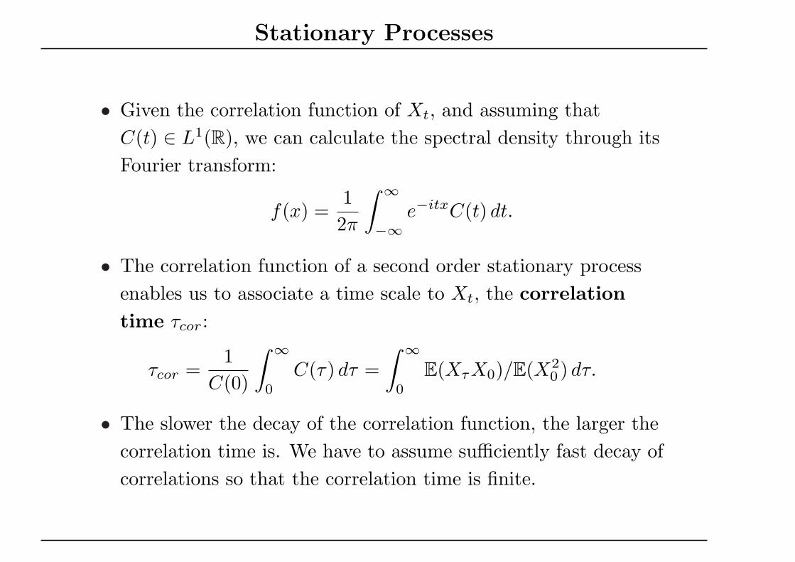
• Given the correlation function of Xt, and assuming thatC(t) ∈ L1(R), we can calculate the spectral density through itsFourier transform:

f(x) =12π

∫ ∞

−∞e−itxC(t) dt.

• The correlation function of a second order stationary processenables us to associate a time scale to Xt, the correlationtime τcor:

τcor =1

C(0)

∫ ∞

0

C(τ) dτ =∫ ∞

0

E(XτX0)/E(X20 ) dτ.

• The slower the decay of the correlation function, the larger thecorrelation time is. We have to assume sufficiently fast decay ofcorrelations so that the correlation time is finite.

Stationary Processes

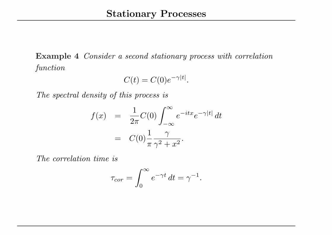
Example 4 Consider a second stationary process with correlationfunction

C(t) = C(0)e−γ|t|.

The spectral density of this process is

f(x) =12π

C(0)∫ ∞

−∞e−itxe−γ|t| dt

= C(0)1π

γ

γ2 + x2.

The correlation time is

τcor =∫ ∞

0

e−γt dt = γ−1.

Gaussian Processes

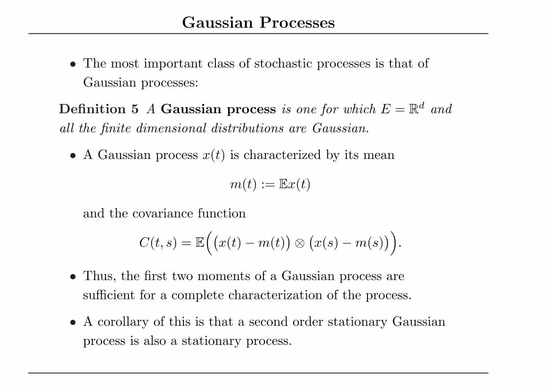
• The most important class of stochastic processes is that ofGaussian processes:

Definition 5 A Gaussian process is one for which E = Rd andall the finite dimensional distributions are Gaussian.

• A Gaussian process x(t) is characterized by its mean

m(t) := Ex(t)

and the covariance function

C(t, s) = E((

x(t)−m(t))⊗ (

x(s)−m(s)))

.

• Thus, the first two moments of a Gaussian process aresufficient for a complete characterization of the process.

• A corollary of this is that a second order stationary Gaussianprocess is also a stationary process.

Brownian Motion

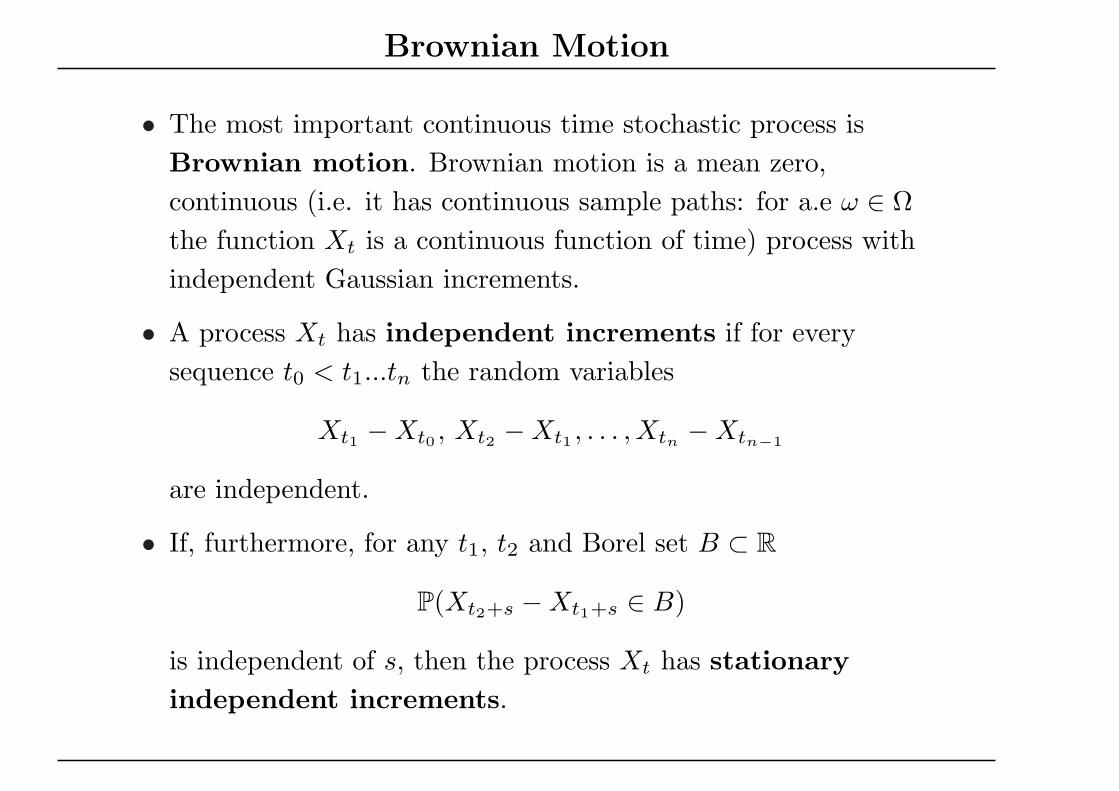
• The most important continuous time stochastic process isBrownian motion. Brownian motion is a mean zero,continuous (i.e. it has continuous sample paths: for a.e ω ∈ Ωthe function Xt is a continuous function of time) process withindependent Gaussian increments.

• A process Xt has independent increments if for everysequence t0 < t1...tn the random variables

Xt1 −Xt0 , Xt2 −Xt1 , . . . , Xtn −Xtn−1

are independent.

• If, furthermore, for any t1, t2 and Borel set B ⊂ R

P(Xt2+s −Xt1+s ∈ B)

is independent of s, then the process Xt has stationaryindependent increments.

Brownian Motion

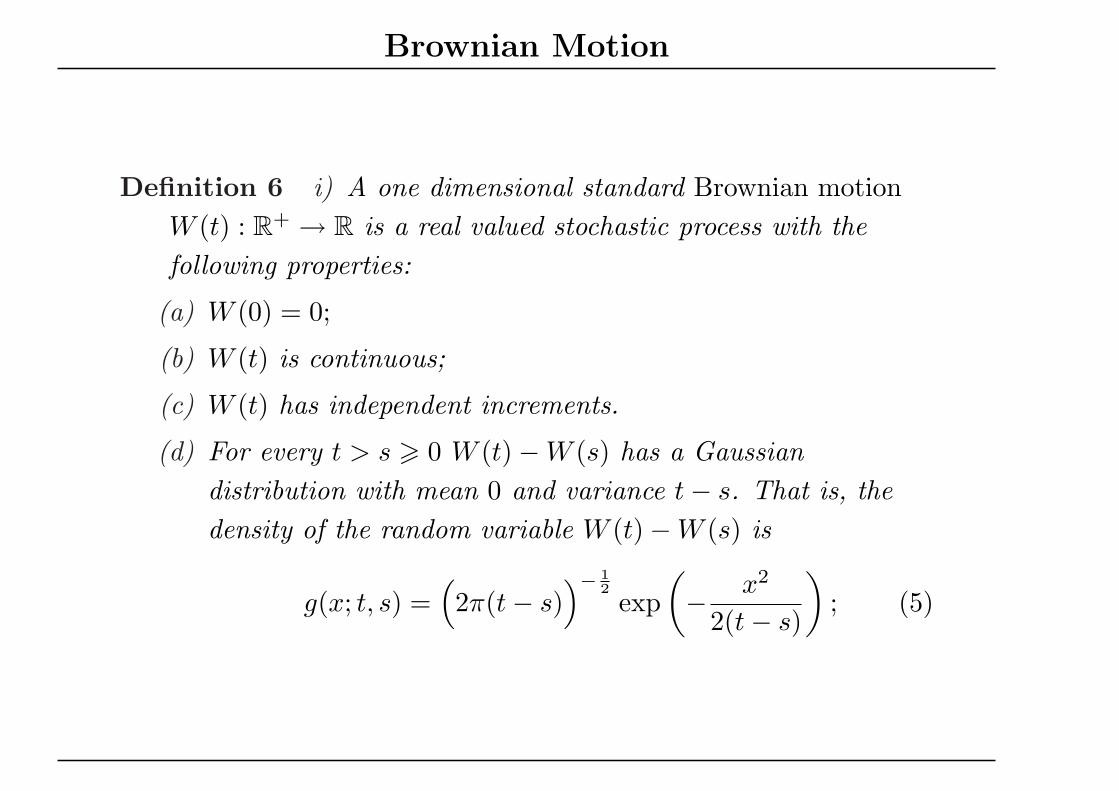
Definition 6 i) A one dimensional standard Brownian motionW (t) : R+ → R is a real valued stochastic process with thefollowing properties:

(a) W (0) = 0;

(b) W (t) is continuous;

(c) W (t) has independent increments.

(d) For every t > s > 0 W (t)−W (s) has a Gaussiandistribution with mean 0 and variance t− s. That is, thedensity of the random variable W (t)−W (s) is

g(x; t, s) =(2π(t− s)

)− 12

exp(− x2

2(t− s)

); (5)

Brownian Motion

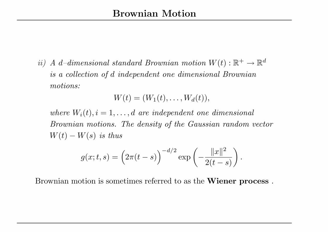
ii) A d–dimensional standard Brownian motion W (t) : R+ → Rd

is a collection of d independent one dimensional Brownianmotions:

W (t) = (W1(t), . . . ,Wd(t)),

where Wi(t), i = 1, . . . , d are independent one dimensionalBrownian motions. The density of the Gaussian random vectorW (t)−W (s) is thus

g(x; t, s) =(2π(t− s)

)−d/2

exp(− ‖x‖2

2(t− s)

).

Brownian motion is sometimes referred to as the Wiener process .

Brownian Motion

0 1 2 3 4 5−4

−3

−2

−1

0

1

2

3

t

W(t)

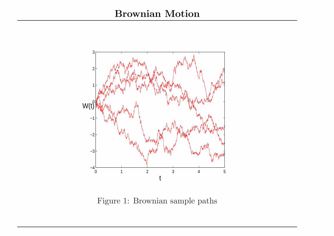
Figure 1: Brownian sample paths

Brownian Motion

It is possible to prove rigorously the existence of the Wienerprocess (Brownian motion):

Theorem 1 (Wiener) There exists an almost-surely continuousprocess Wt with independent increments such and W0 = 0, suchthat for each t > the random variable Wt is N (0, t). Furthermore,Wt is almost surely locally Holder continuous with exponent α forany α ∈ (0, 1

2 ).

Notice that Brownian paths are not differentiable.

Brownian Motion

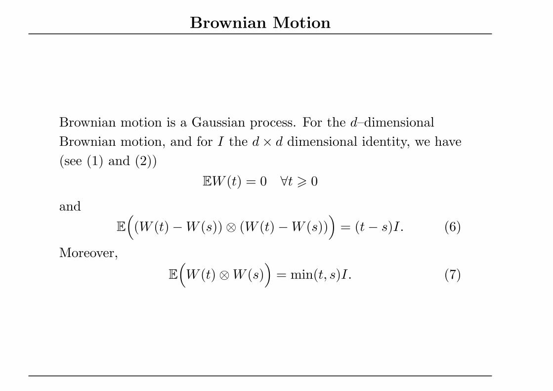
Brownian motion is a Gaussian process. For the d–dimensionalBrownian motion, and for I the d× d dimensional identity, we have(see (1) and (2))

EW (t) = 0 ∀t > 0

andE

((W (t)−W (s))⊗ (W (t)−W (s))

)= (t− s)I. (6)

Moreover,

E(W (t)⊗W (s)

)= min(t, s)I. (7)

Brownian Motion

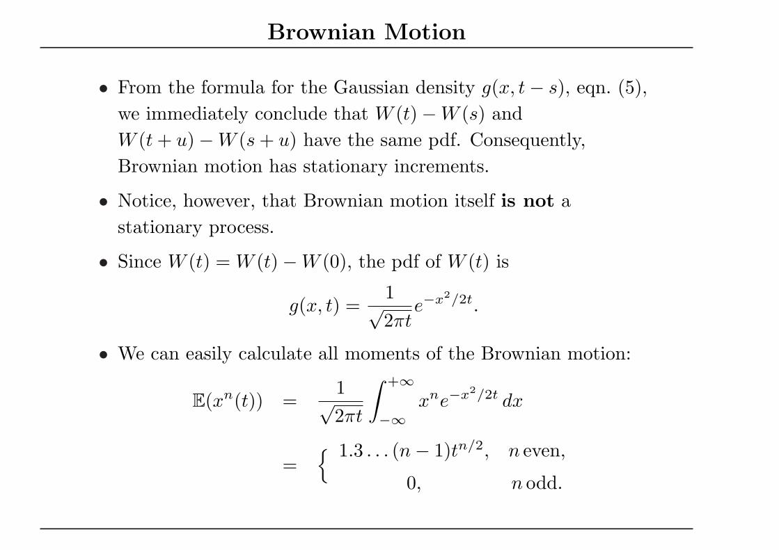
• From the formula for the Gaussian density g(x, t− s), eqn. (5),we immediately conclude that W (t)−W (s) andW (t + u)−W (s + u) have the same pdf. Consequently,Brownian motion has stationary increments.

• Notice, however, that Brownian motion itself is not astationary process.

• Since W (t) = W (t)−W (0), the pdf of W (t) is

g(x, t) =1√2πt

e−x2/2t.

• We can easily calculate all moments of the Brownian motion:

E(xn(t)) =1√2πt

∫ +∞

−∞xne−x2/2t dx

= 1.3 . . . (n− 1)tn/2, n even,

0, n odd.

The Poisson Process

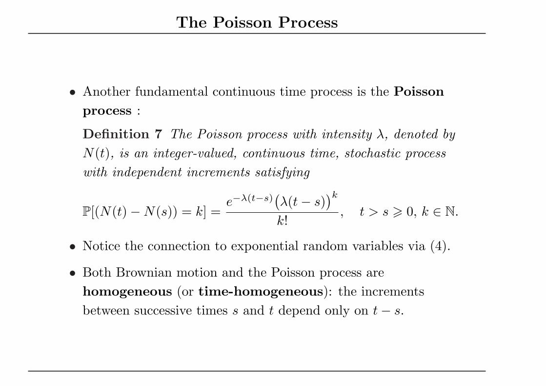
• Another fundamental continuous time process is the Poissonprocess :

Definition 7 The Poisson process with intensity λ, denoted byN(t), is an integer-valued, continuous time, stochastic processwith independent increments satisfying

P[(N(t)−N(s)) = k] =e−λ(t−s)

(λ(t− s)

)k

k!, t > s > 0, k ∈ N.

• Notice the connection to exponential random variables via (4).

• Both Brownian motion and the Poisson process arehomogeneous (or time-homogeneous): the incrementsbetween successive times s and t depend only on t− s.

The Path Space

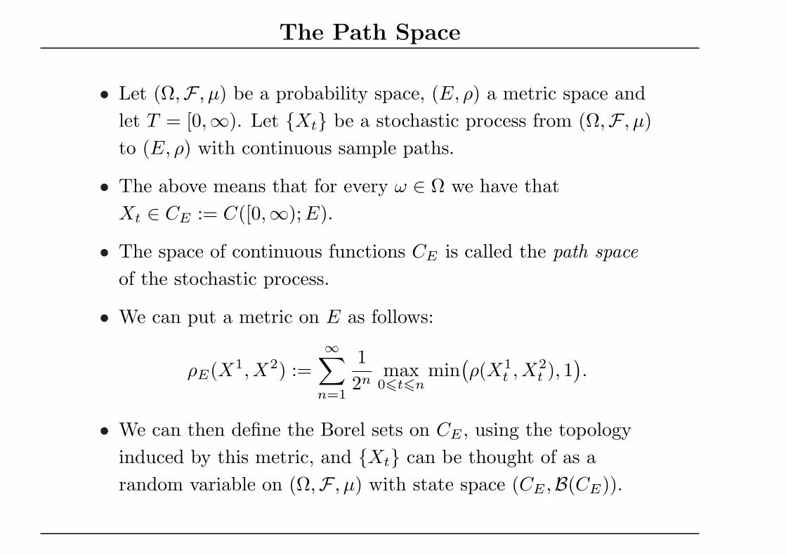
• Let (Ω,F , µ) be a probability space, (E, ρ) a metric space andlet T = [0,∞). Let Xt be a stochastic process from (Ω,F , µ)to (E, ρ) with continuous sample paths.

• The above means that for every ω ∈ Ω we have thatXt ∈ CE := C([0,∞); E).

• The space of continuous functions CE is called the path spaceof the stochastic process.

• We can put a metric on E as follows:

ρE(X1, X2) :=∞∑

n=1

12n

max06t6n

min(ρ(X1

t , X2t ), 1

).

• We can then define the Borel sets on CE , using the topologyinduced by this metric, and Xt can be thought of as arandom variable on (Ω,F , µ) with state space (CE ,B(CE)).

The Path Space

• The probability measure PX−1t on (CE ,B(CE)) is called the

law of Xt.• The law of a stochastic process is a probability measure on its

path space.

Example 8 The space of continuous functions CE is the pathspace of Brownian motion (the Wiener process). The law ofBrownian motion, that is the measure that it induces onC([0,∞),Rd), is known as the Wiener measure.