Eigenvalues - Basicshome.ku.edu.tr/~emengi/teaching/math504_f2011/Lecture21_new.pdfFor any...
97
Basic Definitions Motivation Eigenvalues - Basics Emre Mengi Department of Mathemtics Koç University Istanbul, Turkey December 5th, 2011 Emre Mengi
Transcript of Eigenvalues - Basicshome.ku.edu.tr/~emengi/teaching/math504_f2011/Lecture21_new.pdfFor any...
Basic DefinitionsMotivation
Eigenvalues - Basics
Emre Mengi
Department of MathemticsKoç University
Istanbul, Turkey
December 5th, 2011
Emre Mengi
Basic DefinitionsMotivation
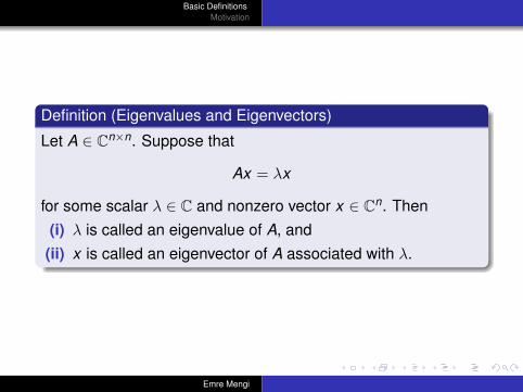
Definition (Eigenvalues and Eigenvectors)
Let A ∈ Cn×n. Suppose that
Ax = λx
for some scalar λ ∈ C and nonzero vector x ∈ Cn. Then(i) λ is called an eigenvalue of A, and
(ii) x is called an eigenvector of A associated with λ.
Emre Mengi
Basic DefinitionsMotivation
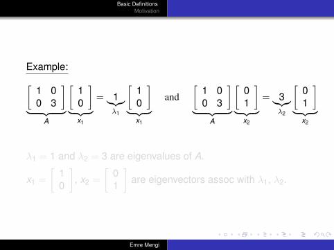
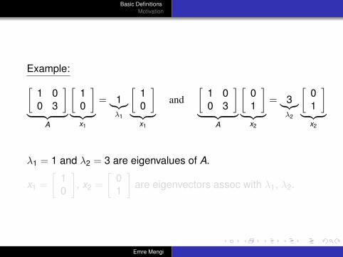
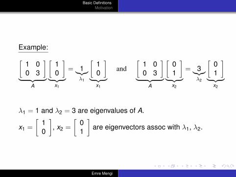
Example:[1 00 3
]︸ ︷︷ ︸
A
[10
]︸ ︷︷ ︸
x1
= 1︸︷︷︸λ1
[10
]︸ ︷︷ ︸
x1
and[
1 00 3
]︸ ︷︷ ︸
A
[01
]︸ ︷︷ ︸
x2
= 3︸︷︷︸λ2
[01
]︸ ︷︷ ︸
x2
λ1 = 1 and λ2 = 3 are eigenvalues of A.
x1 =
[10
], x2 =
[01
]are eigenvectors assoc with λ1, λ2.
Emre Mengi
Basic DefinitionsMotivation
Example:[1 00 3
]︸ ︷︷ ︸
A
[10
]︸ ︷︷ ︸
x1
= 1︸︷︷︸λ1
[10
]︸ ︷︷ ︸
x1
and[
1 00 3
]︸ ︷︷ ︸
A
[01
]︸ ︷︷ ︸
x2
= 3︸︷︷︸λ2
[01
]︸ ︷︷ ︸
x2
λ1 = 1 and λ2 = 3 are eigenvalues of A.
x1 =
[10
], x2 =
[01
]are eigenvectors assoc with λ1, λ2.
Emre Mengi
Basic DefinitionsMotivation
Example:[1 00 3
]︸ ︷︷ ︸
A
[10
]︸ ︷︷ ︸
x1
= 1︸︷︷︸λ1
[10
]︸ ︷︷ ︸
x1
and[
1 00 3
]︸ ︷︷ ︸
A
[01
]︸ ︷︷ ︸
x2
= 3︸︷︷︸λ2
[01
]︸ ︷︷ ︸
x2
λ1 = 1 and λ2 = 3 are eigenvalues of A.
x1 =
[10
], x2 =
[01
]are eigenvectors assoc with λ1, λ2.
Emre Mengi
Basic DefinitionsMotivation
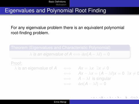
Eigenvalues and Polynomial Root Finding
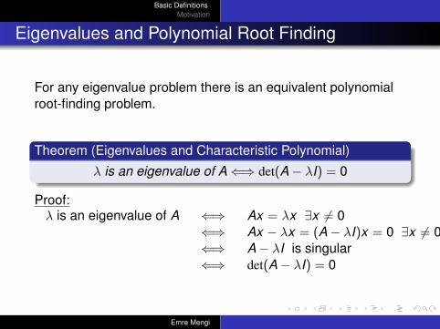
For any eigenvalue problem there is an equivalent polynomialroot-finding problem.
Theorem (Eigenvalues and Characteristic Polynomial)
λ is an eigenvalue of A⇐⇒ det(A− λI) = 0
Proof:λ is an eigenvalue of A ⇐⇒ Ax = λx ∃x 6= 0
⇐⇒ Ax − λx = (A− λI)x = 0 ∃x 6= 0⇐⇒ A− λI is singular⇐⇒ det(A− λI) = 0
Emre Mengi
Basic DefinitionsMotivation
Eigenvalues and Polynomial Root Finding
For any eigenvalue problem there is an equivalent polynomialroot-finding problem.
Theorem (Eigenvalues and Characteristic Polynomial)
λ is an eigenvalue of A⇐⇒ det(A− λI) = 0
Proof:λ is an eigenvalue of A ⇐⇒ Ax = λx ∃x 6= 0
⇐⇒ Ax − λx = (A− λI)x = 0 ∃x 6= 0⇐⇒ A− λI is singular⇐⇒ det(A− λI) = 0
Emre Mengi
Basic DefinitionsMotivation
Eigenvalues and Polynomial Root Finding
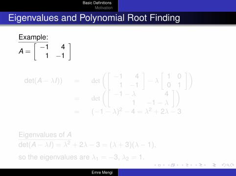
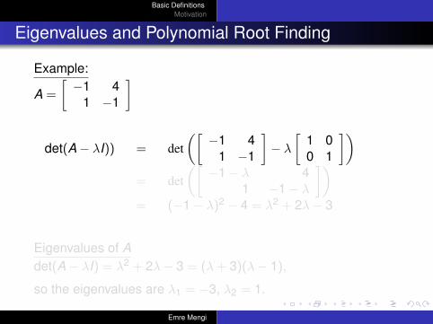
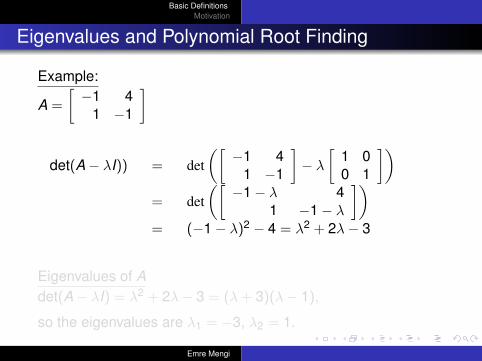
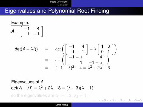
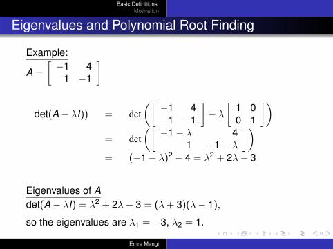
Example:
A =
[−1 4
1 −1
]
det(A− λI)) = det([−1 4
1 −1
]− λ
[1 00 1
])= det
([−1− λ 4
1 −1− λ
])= (−1− λ)2 − 4 = λ2 + 2λ− 3
Eigenvalues of Adet(A− λI) = λ2 + 2λ− 3 = (λ+ 3)(λ− 1),
so the eigenvalues are λ1 = −3, λ2 = 1.
Emre Mengi
Basic DefinitionsMotivation
Eigenvalues and Polynomial Root Finding
Example:
A =
[−1 4
1 −1
]
det(A− λI)) = det([−1 4
1 −1
]− λ
[1 00 1
])= det
([−1− λ 4
1 −1− λ
])= (−1− λ)2 − 4 = λ2 + 2λ− 3
Eigenvalues of Adet(A− λI) = λ2 + 2λ− 3 = (λ+ 3)(λ− 1),
so the eigenvalues are λ1 = −3, λ2 = 1.
Emre Mengi

Basic DefinitionsMotivation
Eigenvalues and Polynomial Root Finding
Example:
A =
[−1 4
1 −1
]
det(A− λI)) = det([−1 4
1 −1
]− λ
[1 00 1
])= det
([−1− λ 4
1 −1− λ
])= (−1− λ)2 − 4 = λ2 + 2λ− 3
Eigenvalues of Adet(A− λI) = λ2 + 2λ− 3 = (λ+ 3)(λ− 1),
so the eigenvalues are λ1 = −3, λ2 = 1.
Emre Mengi
Basic DefinitionsMotivation
Eigenvalues and Polynomial Root Finding
Example:
A =
[−1 4
1 −1
]
det(A− λI)) = det([−1 4
1 −1
]− λ
[1 00 1
])= det
([−1− λ 4
1 −1− λ
])= (−1− λ)2 − 4 = λ2 + 2λ− 3
Eigenvalues of Adet(A− λI) = λ2 + 2λ− 3 = (λ+ 3)(λ− 1),
so the eigenvalues are λ1 = −3, λ2 = 1.
Emre Mengi
Basic DefinitionsMotivation
Eigenvalues and Polynomial Root Finding
Example:
A =
[−1 4
1 −1
]
det(A− λI)) = det([−1 4
1 −1
]− λ
[1 00 1
])= det
([−1− λ 4
1 −1− λ
])= (−1− λ)2 − 4 = λ2 + 2λ− 3
Eigenvalues of Adet(A− λI) = λ2 + 2λ− 3 = (λ+ 3)(λ− 1),
so the eigenvalues are λ1 = −3, λ2 = 1.
Emre Mengi
Basic DefinitionsMotivation
Eigenvalues and Polynomial Root Finding
Example:
A =
[−1 4
1 −1
]
det(A− λI)) = det([−1 4
1 −1
]− λ
[1 00 1
])= det
([−1− λ 4
1 −1− λ
])= (−1− λ)2 − 4 = λ2 + 2λ− 3
Eigenvalues of Adet(A− λI) = λ2 + 2λ− 3 = (λ+ 3)(λ− 1),
so the eigenvalues are λ1 = −3, λ2 = 1.
Emre Mengi
Basic DefinitionsMotivation
Eigenvalues and Polynomial Root Finding
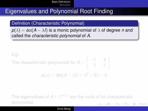
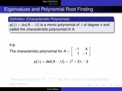
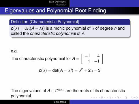
Definition (Characteristic Polynomial)
p(λ) = det(A− λI) is a monic polynomial of λ of degree n andcalled the characteristic polynomial of A.
e.g.
The characteristic polynomial for A =
[−1 4
1 −1
]p(λ) = det(A− λI) = λ2 + 2λ− 3
The eigenvalues of A ∈ Cn×n are the roots of its characteristicpolynomial.
Emre Mengi
Basic DefinitionsMotivation
Eigenvalues and Polynomial Root Finding
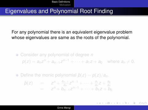
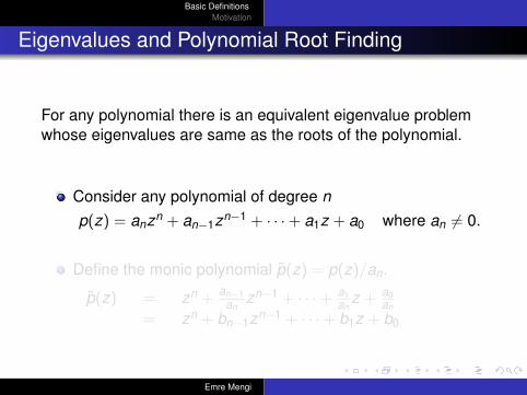
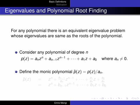
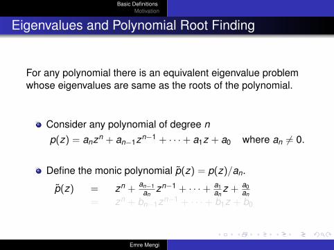
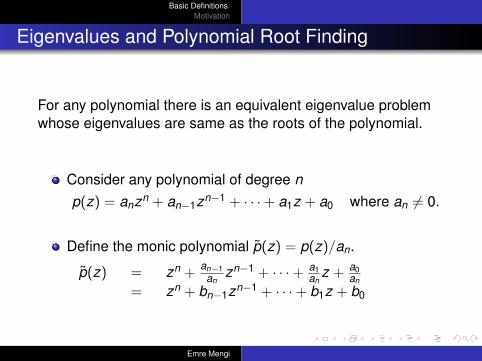
For any polynomial there is an equivalent eigenvalue problemwhose eigenvalues are same as the roots of the polynomial.
Consider any polynomial of degree np(z) = anzn + an−1zn−1 + · · ·+ a1z + a0 where an 6= 0.
Define the monic polynomial p̃(z) = p(z)/an.
p̃(z) = zn +an−1
anzn−1 + · · ·+ a1
anz + a0
an
= zn + bn−1zn−1 + · · ·+ b1z + b0
Emre Mengi
Basic DefinitionsMotivation
Eigenvalues and Polynomial Root Finding
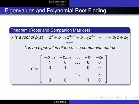
Theorem (Roots and Companion Matrices)
λ is a root of p̃(z) = zn + bn−1zn−1 + bn−2zn−2 + · · ·+ b1z + b0⇐⇒
λ is an eigenvalue of the n × n companion matrix
C =
−bn−1 −bn−2 . . . −b1 −b0
1 0 . . . 0 00 1 0 0...
. . ....
0 0 1 0
Emre Mengi
Basic DefinitionsMotivation
Eigenvalues and Polynomial Root Finding
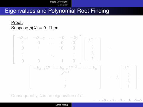
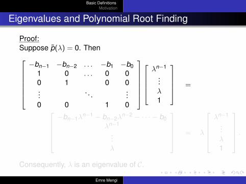
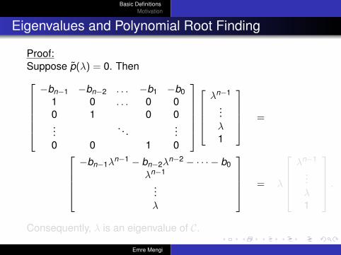
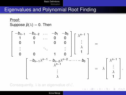
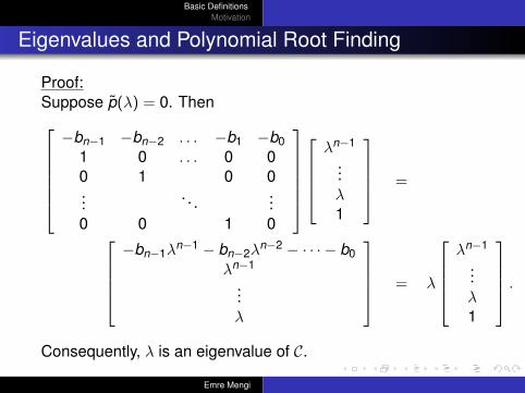
Proof:Suppose p̃(λ) = 0. Then−bn−1 −bn−2 . . . −b1 −b0
1 0 . . . 0 00 1 0 0...
. . ....
0 0 1 0
λn−1
...λ1
=
−bn−1λ
n−1 − bn−2λn−2 − · · · − b0
λn−1
...λ
= λ
λn−1
...λ1
.Consequently, λ is an eigenvalue of C.
Emre Mengi
Basic DefinitionsMotivation
Eigenvalues and Polynomial Root Finding
Proof:Suppose p̃(λ) = 0. Then−bn−1 −bn−2 . . . −b1 −b0
1 0 . . . 0 00 1 0 0...
. . ....
0 0 1 0
λn−1
...λ1
=
−bn−1λ
n−1 − bn−2λn−2 − · · · − b0
λn−1
...λ
= λ
λn−1
...λ1
.Consequently, λ is an eigenvalue of C.
Emre Mengi
Basic DefinitionsMotivation
Eigenvalues and Polynomial Root Finding
Proof:Suppose p̃(λ) = 0. Then−bn−1 −bn−2 . . . −b1 −b0
1 0 . . . 0 00 1 0 0...
. . ....
0 0 1 0
λn−1
...λ1
=
−bn−1λ
n−1 − bn−2λn−2 − · · · − b0
λn−1
...λ
= λ
λn−1
...λ1
.Consequently, λ is an eigenvalue of C.
Emre Mengi
Basic DefinitionsMotivation
Eigenvalues and Polynomial Root Finding
Proof:Suppose p̃(λ) = 0. Then−bn−1 −bn−2 . . . −b1 −b0
1 0 . . . 0 00 1 0 0...
. . ....
0 0 1 0
λn−1
...λ1
=
−bn−1λ
n−1 − bn−2λn−2 − · · · − b0
λn−1
...λ
= λ
λn−1
...λ1
.Consequently, λ is an eigenvalue of C.
Emre Mengi
Basic DefinitionsMotivation
Eigenvalues and Polynomial Root Finding
Proof:Suppose p̃(λ) = 0. Then−bn−1 −bn−2 . . . −b1 −b0
1 0 . . . 0 00 1 0 0...
. . ....
0 0 1 0
λn−1
...λ1
=
−bn−1λ
n−1 − bn−2λn−2 − · · · − b0
λn−1
...λ
= λ
λn−1
...λ1
.Consequently, λ is an eigenvalue of C.
Emre Mengi
Basic DefinitionsMotivation
Eigenvalues and Polynomial Root Finding
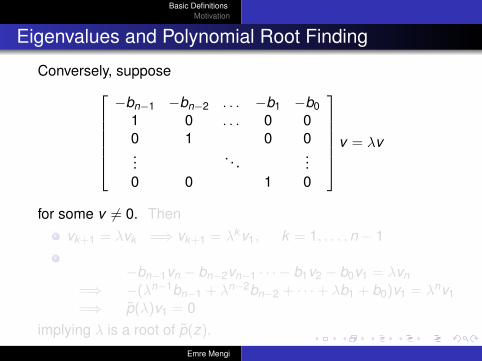
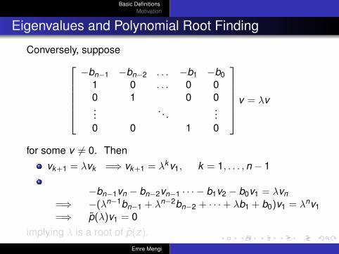
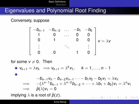
Conversely, suppose−bn−1 −bn−2 . . . −b1 −b0
1 0 . . . 0 00 1 0 0...
. . ....
0 0 1 0
v = λv
for some v 6= 0. Thenvk+1 = λvk =⇒ vk+1 = λkv1, k = 1, . . . ,n − 1
−bn−1vn − bn−2vn−1 · · · − b1v2 − b0v1 = λvn=⇒ −(λn−1bn−1 + λn−2bn−2 + · · ·+ λb1 + b0)v1 = λnv1=⇒ p̃(λ)v1 = 0
implying λ is a root of p̃(z).Emre Mengi
Basic DefinitionsMotivation
Eigenvalues and Polynomial Root Finding
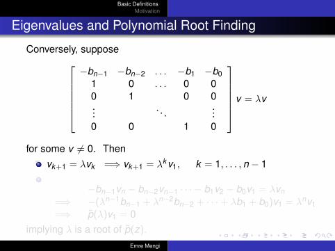
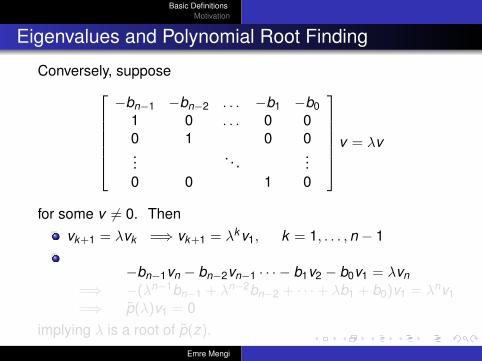
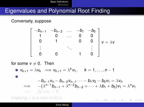
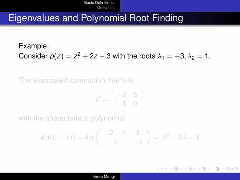
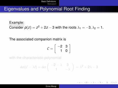
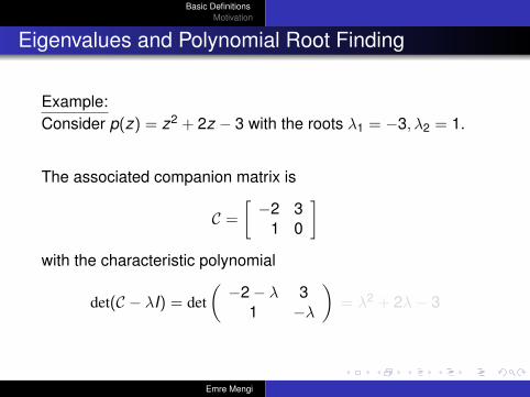
Example:Consider p(z) = z2 + 2z − 3 with the roots λ1 = −3, λ2 = 1.
The associated companion matrix is
C =[−2 3
1 0
]with the characteristic polynomial
det(C − λI) = det(−2− λ 3
1 −λ
)= λ2 + 2λ− 3
Emre Mengi
Basic DefinitionsMotivation
Eigenvalues and Polynomial Root Finding
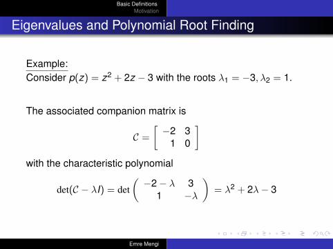
Example:Consider p(z) = z2 + 2z − 3 with the roots λ1 = −3, λ2 = 1.
The associated companion matrix is
C =[−2 3
1 0
]with the characteristic polynomial
det(C − λI) = det(−2− λ 3
1 −λ
)= λ2 + 2λ− 3
Emre Mengi
Basic DefinitionsMotivation
Eigenvalues and Polynomial Root Finding
Example:Consider p(z) = z2 + 2z − 3 with the roots λ1 = −3, λ2 = 1.
The associated companion matrix is
C =[−2 3
1 0
]with the characteristic polynomial
det(C − λI) = det(−2− λ 3
1 −λ
)= λ2 + 2λ− 3
Emre Mengi
Basic DefinitionsMotivation
Eigenvalues and Polynomial Root Finding
Example:Consider p(z) = z2 + 2z − 3 with the roots λ1 = −3, λ2 = 1.
The associated companion matrix is
C =[−2 3
1 0
]with the characteristic polynomial
det(C − λI) = det(−2− λ 3
1 −λ
)= λ2 + 2λ− 3
Emre Mengi
Basic DefinitionsMotivation
Eigenvalues and Polynomial Root Finding
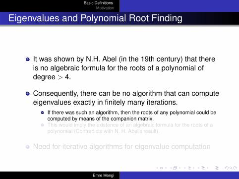
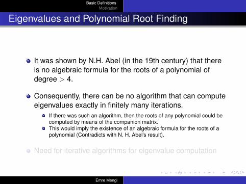
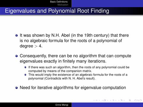
It was shown by N.H. Abel (in the 19th century) that thereis no algebraic formula for the roots of a polynomial ofdegree > 4.
Consequently, there can be no algorithm that can computeeigenvalues exactly in finitely many iterations.
If there was such an algorithm, then the roots of any polynomial could becomputed by means of the companion matrix.This would imply the existence of an algebraic formula for the roots of apolynomial (Contradicts with N. H. Abel’s result).
Need for iterative algorithms for eigenvalue computation
Emre Mengi
Basic DefinitionsMotivation
Eigenvalues and Polynomial Root Finding
It was shown by N.H. Abel (in the 19th century) that thereis no algebraic formula for the roots of a polynomial ofdegree > 4.
Consequently, there can be no algorithm that can computeeigenvalues exactly in finitely many iterations.
If there was such an algorithm, then the roots of any polynomial could becomputed by means of the companion matrix.This would imply the existence of an algebraic formula for the roots of apolynomial (Contradicts with N. H. Abel’s result).
Need for iterative algorithms for eigenvalue computation
Emre Mengi
Basic DefinitionsMotivation
Algebraic Multiplicity
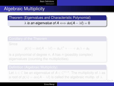
Theorem (Eigenvalues and Characteristic Polynomial)
λ is an eigenvalue of A⇐⇒ det(A− λI) = 0
Corollary of the TheoremSince
p(λ) = det(A− λI) = anλn + · · ·+ a1λ+ a0
is a polynomial of degree n, A has n (possibly complex)eigenvalues (counting the multiplicities).
Definition (Algebraic Multiplicity)
Let λ ∈ C be an eigenvalue of A ∈ Cn×n. The multiplicity of λ asa root of p(λ) = det(A− λI) is called the algebraic multip. of λ.
Emre Mengi
Basic DefinitionsMotivation
Algebraic Multiplicity
Theorem (Eigenvalues and Characteristic Polynomial)
λ is an eigenvalue of A⇐⇒ det(A− λI) = 0
Corollary of the TheoremSince
p(λ) = det(A− λI) = anλn + · · ·+ a1λ+ a0
is a polynomial of degree n, A has n (possibly complex)eigenvalues (counting the multiplicities).
Definition (Algebraic Multiplicity)
Let λ ∈ C be an eigenvalue of A ∈ Cn×n. The multiplicity of λ asa root of p(λ) = det(A− λI) is called the algebraic multip. of λ.
Emre Mengi
Basic DefinitionsMotivation
Calculation of Eigenvectors
Calculation of Eigenvectors
Let λ ∈ C be an eigenvalue of A ∈ Cn×n.Then v is an eigenvector associated with λ⇐⇒ (A− λI)v = 0and v 6= 0.
Example:
The matrix A =
[−1 4
1 −1
]has eigenvalues λ1 = −3, λ2 = 1.
Emre Mengi
Basic DefinitionsMotivation
Calculation of Eigenvectors
Calculation of Eigenvectors
Let λ ∈ C be an eigenvalue of A ∈ Cn×n.Then v is an eigenvector associated with λ⇐⇒ (A− λI)v = 0and v 6= 0.
Example:
The matrix A =
[−1 4
1 −1
]has eigenvalues λ1 = −3, λ2 = 1.
Emre Mengi
Basic DefinitionsMotivation
Calculation of Eigenvectors
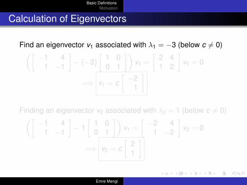
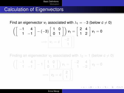
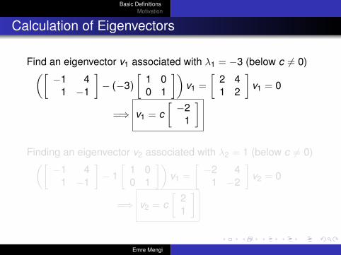
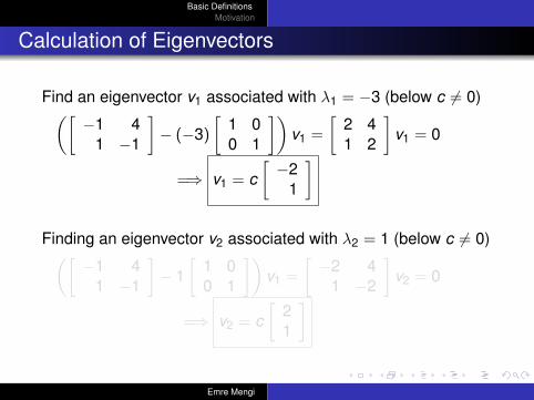
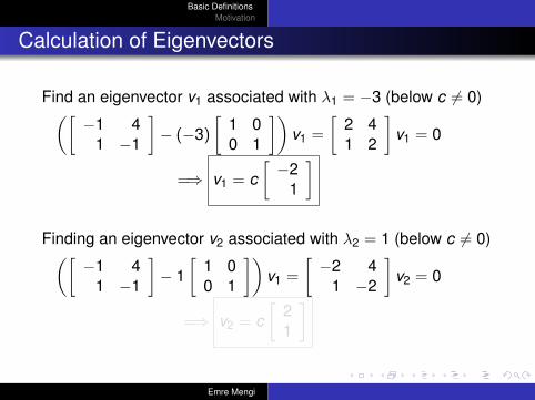
Find an eigenvector v1 associated with λ1 = −3 (below c 6= 0)([−1 4
1 −1
]− (−3)
[1 00 1
])v1 =
[2 41 2
]v1 = 0
=⇒ v1 = c[−2
1
]
Finding an eigenvector v2 associated with λ2 = 1 (below c 6= 0)([−1 4
1 −1
]− 1
[1 00 1
])v1 =
[−2 4
1 −2
]v2 = 0
=⇒ v2 = c[
21
]
Emre Mengi
Basic DefinitionsMotivation
Calculation of Eigenvectors
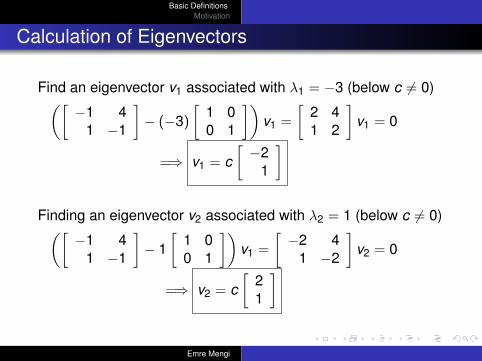
Find an eigenvector v1 associated with λ1 = −3 (below c 6= 0)([−1 4
1 −1
]− (−3)
[1 00 1
])v1 =
[2 41 2
]v1 = 0
=⇒ v1 = c[−2
1
]
Finding an eigenvector v2 associated with λ2 = 1 (below c 6= 0)([−1 4
1 −1
]− 1
[1 00 1
])v1 =
[−2 4
1 −2
]v2 = 0
=⇒ v2 = c[
21
]
Emre Mengi
Basic DefinitionsMotivation
Eigenspace
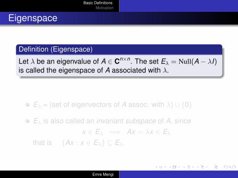
Definition (Eigenspace)
Let λ be an eigenvalue of A ∈ Cn×n. The set Eλ = Null(A− λI)is called the eigenspace of A associated with λ.
Eλ = (set of eigenvectors of A assoc. with λ) ∪ {0}
Eλ is also called an invariant subspace of A, sincex ∈ Eλ =⇒ Ax = λx ∈ Eλ
that is {Ax : x ∈ Eλ} ⊆ Eλ.
Emre Mengi
Basic DefinitionsMotivation
Eigenspace
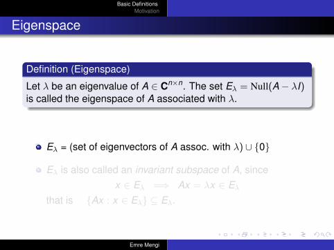
Definition (Eigenspace)
Let λ be an eigenvalue of A ∈ Cn×n. The set Eλ = Null(A− λI)is called the eigenspace of A associated with λ.
Eλ = (set of eigenvectors of A assoc. with λ) ∪ {0}
Eλ is also called an invariant subspace of A, sincex ∈ Eλ =⇒ Ax = λx ∈ Eλ
that is {Ax : x ∈ Eλ} ⊆ Eλ.
Emre Mengi
Basic DefinitionsMotivation
Eigenspace
Definition (Eigenspace)
Let λ be an eigenvalue of A ∈ Cn×n. The set Eλ = Null(A− λI)is called the eigenspace of A associated with λ.
Eλ = (set of eigenvectors of A assoc. with λ) ∪ {0}
Eλ is also called an invariant subspace of A, sincex ∈ Eλ =⇒ Ax = λx ∈ Eλ
that is {Ax : x ∈ Eλ} ⊆ Eλ.
Emre Mengi
Basic DefinitionsMotivation
Geometric Multiplicity
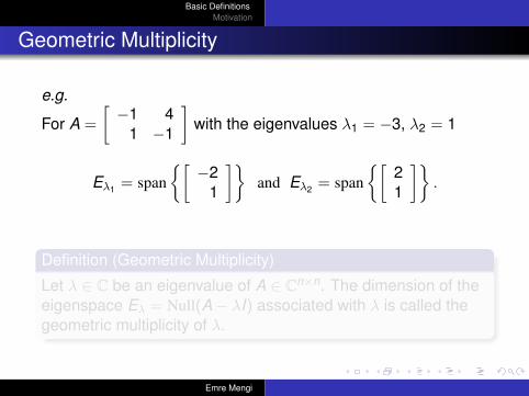
e.g.
For A =
[−1 4
1 −1
]with the eigenvalues λ1 = −3, λ2 = 1
Eλ1 = span{[−2
1
]}and Eλ2 = span
{[21
]}.
Definition (Geometric Multiplicity)
Let λ ∈ C be an eigenvalue of A ∈ Cn×n. The dimension of theeigenspace Eλ = Null(A− λI) associated with λ is called thegeometric multiplicity of λ.
Emre Mengi
Basic DefinitionsMotivation
Geometric Multiplicity
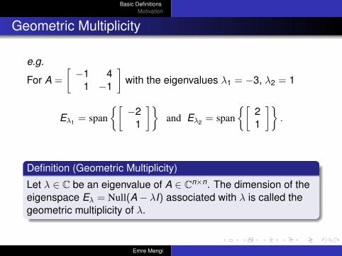
e.g.
For A =
[−1 4
1 −1
]with the eigenvalues λ1 = −3, λ2 = 1
Eλ1 = span{[−2
1
]}and Eλ2 = span
{[21
]}.
Definition (Geometric Multiplicity)
Let λ ∈ C be an eigenvalue of A ∈ Cn×n. The dimension of theeigenspace Eλ = Null(A− λI) associated with λ is called thegeometric multiplicity of λ.
Emre Mengi
Basic DefinitionsMotivation
Geometric Multiplicity
e.g.
For A =
[−1 4
1 −1
]with the eigenvalues λ1 = −3, λ2 = 1
Eλ1 = span{[−2
1
]}and Eλ2 = span
{[21
]}.
Definition (Geometric Multiplicity)
Let λ ∈ C be an eigenvalue of A ∈ Cn×n. The dimension of theeigenspace Eλ = Null(A− λI) associated with λ is called thegeometric multiplicity of λ.
Emre Mengi
Basic DefinitionsMotivation
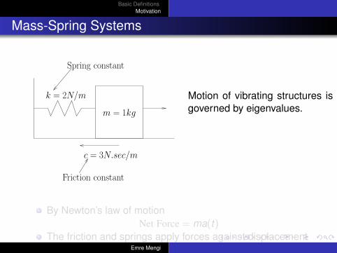
Mass-Spring Systems
c = 3N.sec/m
Spring constant
Friction constant
m = 1kg
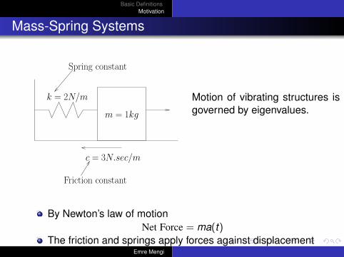
k = 2N/m Motion of vibrating structures isgoverned by eigenvalues.
By Newton’s law of motionNet Force = ma(t)
The friction and springs apply forces against displacementNet Force = −c v(t)− k x(t)Emre Mengi
Basic DefinitionsMotivation
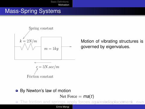
Mass-Spring Systems
c = 3N.sec/m
Spring constant
Friction constant
m = 1kg
k = 2N/m Motion of vibrating structures isgoverned by eigenvalues.
By Newton’s law of motionNet Force = ma(t)
The friction and springs apply forces against displacementNet Force = −c v(t)− k x(t)Emre Mengi
Basic DefinitionsMotivation
Mass Spring Systems
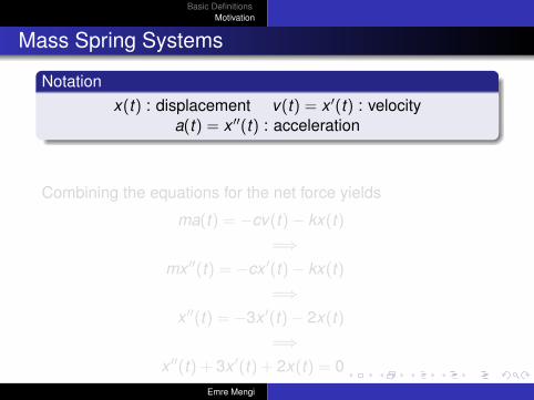
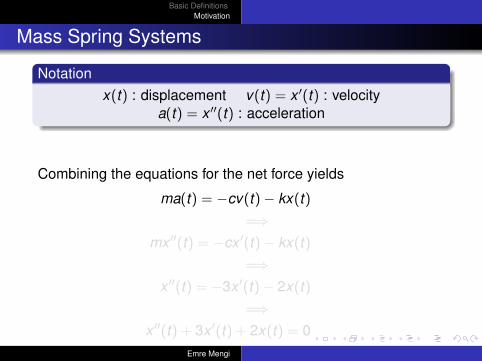
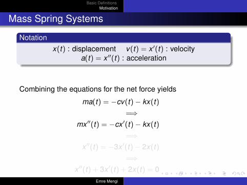
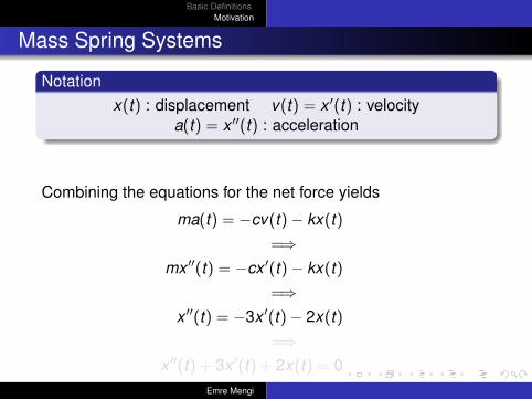
Notationx(t) : displacement v(t) = x ′(t) : velocity
a(t) = x ′′(t) : acceleration
Combining the equations for the net force yields
ma(t) = −cv(t)− kx(t)=⇒
mx ′′(t) = −cx ′(t)− kx(t)=⇒
x ′′(t) = −3x ′(t)− 2x(t)=⇒
x ′′(t) + 3x ′(t) + 2x(t) = 0Emre Mengi
Basic DefinitionsMotivation
Mass Spring Systems
Notationx(t) : displacement v(t) = x ′(t) : velocity
a(t) = x ′′(t) : acceleration
Combining the equations for the net force yields
ma(t) = −cv(t)− kx(t)=⇒
mx ′′(t) = −cx ′(t)− kx(t)=⇒
x ′′(t) = −3x ′(t)− 2x(t)=⇒
x ′′(t) + 3x ′(t) + 2x(t) = 0Emre Mengi
Basic DefinitionsMotivation
Mass Spring Systems
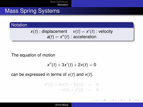
Notationx(t) : displacement v(t) = x ′(t) : velocity
a(t) = x ′′(t) : acceleration
The equation of motion
x ′′(t) + 3x ′(t) + 2x(t) = 0
can be expressed in terms of v(t) and x(t).
v ′(t) + 3v(t) + 2x(t) = 0−v(t) + x ′(t) = 0
Emre Mengi

Basic DefinitionsMotivation
Mass Spring Systems
Notationx(t) : displacement v(t) = x ′(t) : velocity
a(t) = x ′′(t) : acceleration
The equation of motion
x ′′(t) + 3x ′(t) + 2x(t) = 0
can be expressed in terms of v(t) and x(t).
v ′(t) + 3v(t) + 2x(t) = 0−v(t) + x ′(t) = 0
Emre Mengi
Basic DefinitionsMotivation
Mass Spring Systems
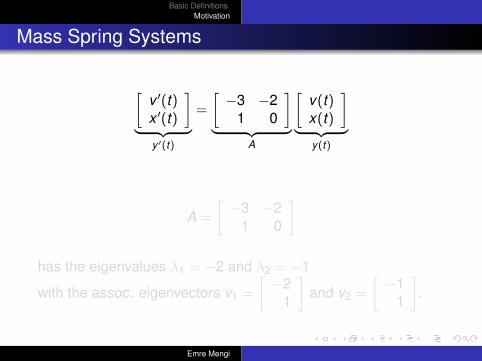
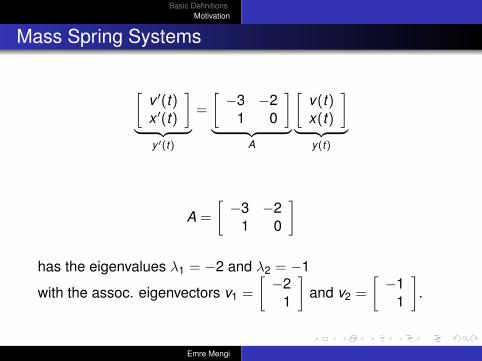
[v ′(t)x ′(t)
]︸ ︷︷ ︸
y ′(t)
=
[−3 −2
1 0
]︸ ︷︷ ︸
A
[v(t)x(t)
]︸ ︷︷ ︸
y(t)
A =
[−3 −2
1 0
]
has the eigenvalues λ1 = −2 and λ2 = −1
with the assoc. eigenvectors v1 =
[−2
1
]and v2 =
[−1
1
].
Emre Mengi
Basic DefinitionsMotivation
Mass Spring Systems
[v ′(t)x ′(t)
]︸ ︷︷ ︸
y ′(t)
=
[−3 −2
1 0
]︸ ︷︷ ︸
A
[v(t)x(t)
]︸ ︷︷ ︸
y(t)
A =
[−3 −2
1 0
]
has the eigenvalues λ1 = −2 and λ2 = −1
with the assoc. eigenvectors v1 =
[−2
1
]and v2 =
[−1
1
].
Emre Mengi
Basic DefinitionsMotivation
Mass Spring Systems
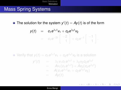
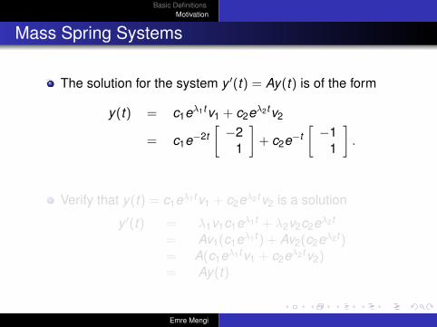
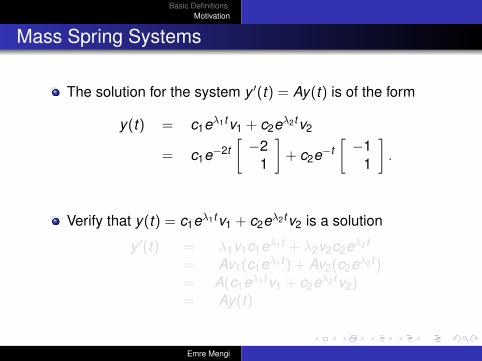
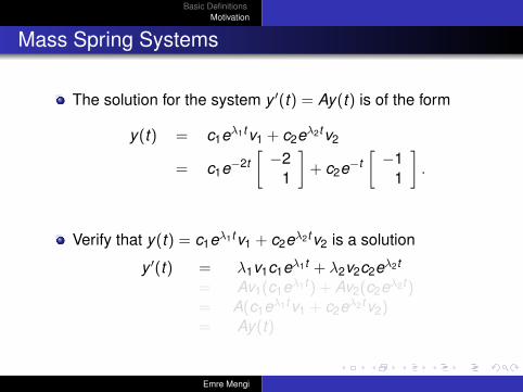
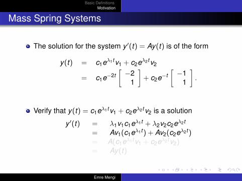
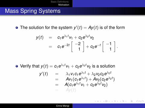
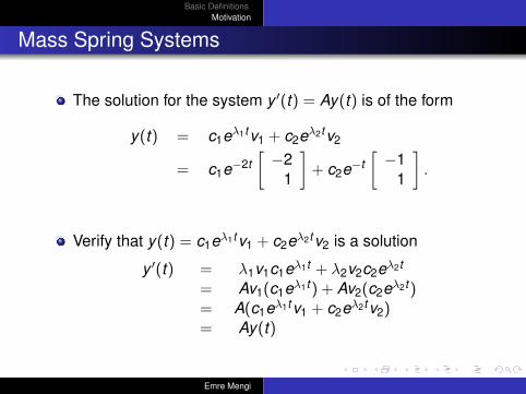
The solution for the system y ′(t) = Ay(t) is of the form
y(t) = c1eλ1tv1 + c2eλ2tv2
= c1e−2t[−2
1
]+ c2e−t
[−1
1
].
Verify that y(t) = c1eλ1tv1 + c2eλ2tv2 is a solution
y ′(t) = λ1v1c1eλ1t + λ2v2c2eλ2t
= Av1(c1eλ1t) + Av2(c2eλ2t)= A(c1eλ1tv1 + c2eλ2tv2)= Ay(t)
Emre Mengi
Basic DefinitionsMotivation
Mass Spring Systems
The solution for the system y ′(t) = Ay(t) is of the form
y(t) = c1eλ1tv1 + c2eλ2tv2
= c1e−2t[−2
1
]+ c2e−t
[−1
1
].
Verify that y(t) = c1eλ1tv1 + c2eλ2tv2 is a solution
y ′(t) = λ1v1c1eλ1t + λ2v2c2eλ2t
= Av1(c1eλ1t) + Av2(c2eλ2t)= A(c1eλ1tv1 + c2eλ2tv2)= Ay(t)
Emre Mengi
Basic DefinitionsMotivation
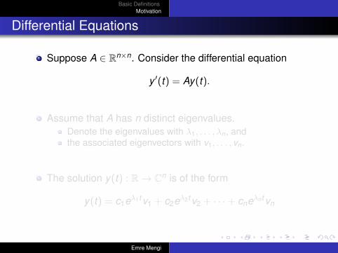
Differential Equations
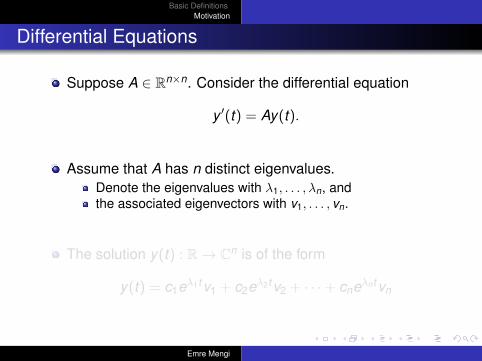
Suppose A ∈ Rn×n. Consider the differential equation
y ′(t) = Ay(t).
Assume that A has n distinct eigenvalues.Denote the eigenvalues with λ1, . . . , λn, andthe associated eigenvectors with v1, . . . , vn.
The solution y(t) : R→ Cn is of the form
y(t) = c1eλ1tv1 + c2eλ2tv2 + · · ·+ cneλntvn
Emre Mengi
Basic DefinitionsMotivation
Differential Equations
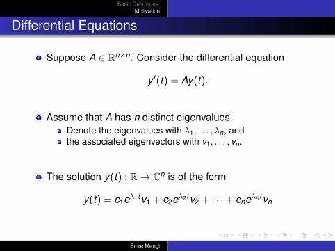
Suppose A ∈ Rn×n. Consider the differential equation
y ′(t) = Ay(t).
Assume that A has n distinct eigenvalues.Denote the eigenvalues with λ1, . . . , λn, andthe associated eigenvectors with v1, . . . , vn.
The solution y(t) : R→ Cn is of the form
y(t) = c1eλ1tv1 + c2eλ2tv2 + · · ·+ cneλntvn
Emre Mengi
Basic DefinitionsMotivation
Differential Equations
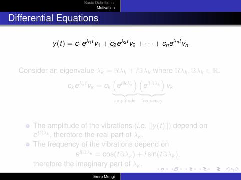
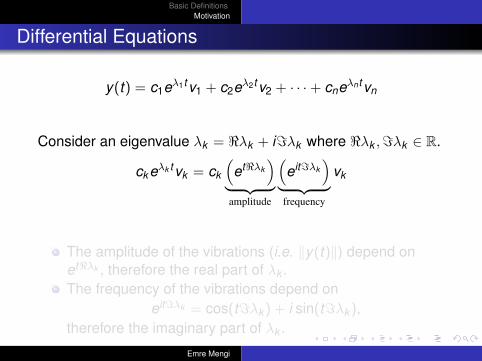
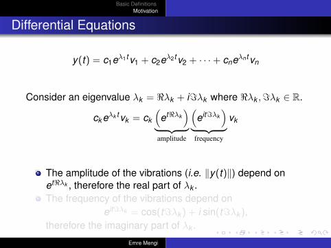
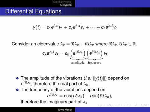
y(t) = c1eλ1tv1 + c2eλ2tv2 + · · ·+ cneλntvn
Consider an eigenvalue λk = <λk + i=λk where <λk ,=λk ∈ R.
ckeλk tvk = ck
(et<λk
)︸ ︷︷ ︸amplitude
(eit=λk
)︸ ︷︷ ︸frequency
vk
The amplitude of the vibrations (i.e. ‖y(t)‖) depend onet<λk , therefore the real part of λk .The frequency of the vibrations depend on
eit=λk = cos(t=λk ) + i sin(t=λk ),therefore the imaginary part of λk .
Emre Mengi
Basic DefinitionsMotivation
Differential Equations
y(t) = c1eλ1tv1 + c2eλ2tv2 + · · ·+ cneλntvn
Consider an eigenvalue λk = <λk + i=λk where <λk ,=λk ∈ R.
ckeλk tvk = ck
(et<λk
)︸ ︷︷ ︸amplitude
(eit=λk
)︸ ︷︷ ︸frequency
vk
The amplitude of the vibrations (i.e. ‖y(t)‖) depend onet<λk , therefore the real part of λk .The frequency of the vibrations depend on
eit=λk = cos(t=λk ) + i sin(t=λk ),therefore the imaginary part of λk .
Emre Mengi
Basic DefinitionsMotivation
Stability
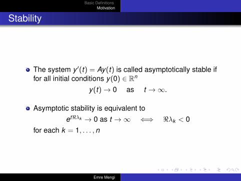
The system y ′(t) = Ay(t) is called asymptotically stable iffor all initial conditions y(0) ∈ Rn
y(t)→ 0 as t →∞.
Asymptotic stability is equivalent toet<λk → 0 as t →∞ ⇐⇒ <λk < 0
for each k = 1, . . . ,n
Emre Mengi
Basic DefinitionsMotivation
Stability
The system y ′(t) = Ay(t) is called asymptotically stable iffor all initial conditions y(0) ∈ Rn
y(t)→ 0 as t →∞.
Asymptotic stability is equivalent toet<λk → 0 as t →∞ ⇐⇒ <λk < 0
for each k = 1, . . . ,n
Emre Mengi
Basic DefinitionsMotivation
Stability
The system y ′(t) = Ay(t) is called asymptotically stable iffor all initial conditions y(0) ∈ Rn
y(t)→ 0 as t →∞.
Asymptotic stability is equivalent toet<λk → 0 as t →∞ ⇐⇒ <λk < 0
for each k = 1, . . . ,n
Emre Mengi
Basic DefinitionsMotivation
Stability
Asymptotic Stability
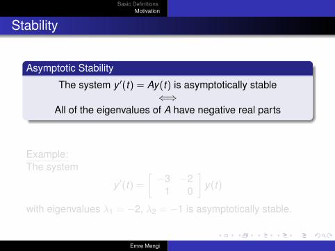
The system y ′(t) = Ay(t) is asymptotically stable⇐⇒
All of the eigenvalues of A have negative real parts
Example:The system
y ′(t) =[−3 −2
1 0
]y(t)
with eigenvalues λ1 = −2, λ2 = −1 is asymptotically stable.
Emre Mengi
Basic DefinitionsMotivation
Stability
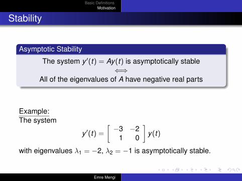
Asymptotic Stability
The system y ′(t) = Ay(t) is asymptotically stable⇐⇒
All of the eigenvalues of A have negative real parts
Example:The system
y ′(t) =[−3 −2
1 0
]y(t)
with eigenvalues λ1 = −2, λ2 = −1 is asymptotically stable.
Emre Mengi

![EIGENVECTORS, EIGENVALUES, AND FINITE STRAIN · unit vector, λ is the length of ... E Eigenvectors have corresponding eigenvalues, and vice-versa F In Matlab, [v,d] = eig(A), ...](https://static.fdocument.org/doc/165x107/5b32041f7f8b9aed688bb633/eigenvectors-eigenvalues-and-finite-strain-unit-vector-is-the-length-of.jpg)