!diversity*metricsevolution.unibas.ch/walser/bacteria_community... ·...
60
αdiversity metrics Markerbased metagenomic tutorial 1
Transcript of !diversity*metricsevolution.unibas.ch/walser/bacteria_community... ·...
α-‐diversity metrics
Marker-‐based metagenomic tutorial 1
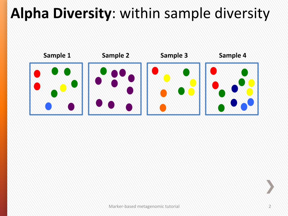
Alpha Diversity: within sample diversity
Sample 1 Sample 2 Sample 3 Sample 4
Marker-‐based metagenomic tutorial 2
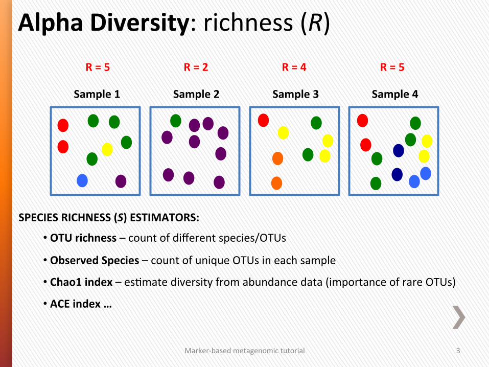
Alpha Diversity: richness (R)
Marker-‐based metagenomic tutorial 3
SPECIES RICHNESS (S) ESTIMATORS:
• OTU richness – count of different species/OTUs
• Observed Species – count of unique OTUs in each sample
• Chao1 index – esGmate diversity from abundance data (importance of rare OTUs)
• ACE index …
Sample 1 Sample 2 Sample 3 Sample 4
R = 5 R = 2 R = 4 R = 5
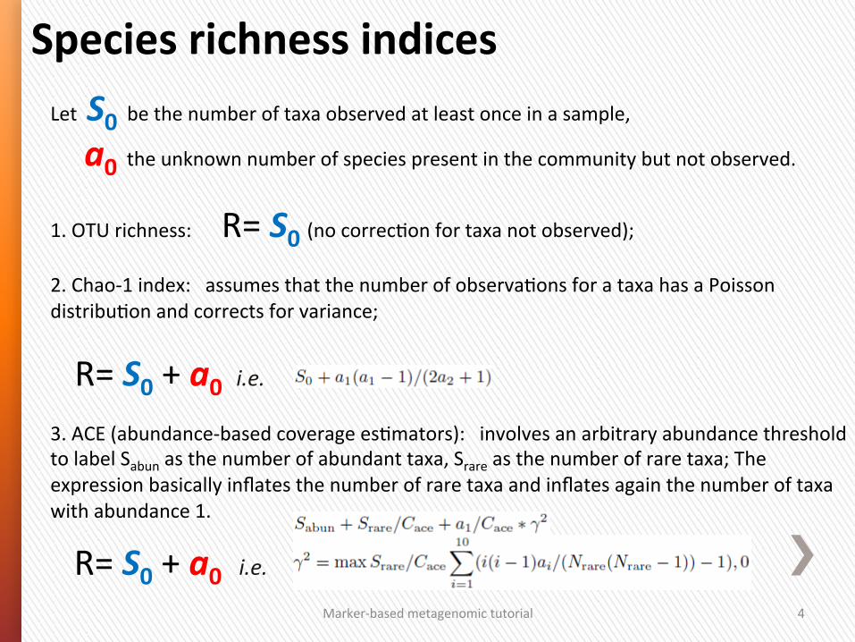
Let S0 be the number of taxa observed at least once in a sample,
a0 the unknown number of species present in the community but not observed.
1. OTU richness: R= S0 (no correcGon for taxa not observed);
2. Chao-‐1 index: assumes that the number of observaGons for a taxa has a Poisson distribuGon and corrects for variance;
R= S0 + a0 i.e. 3. ACE (abundance-‐based coverage esGmators): involves an arbitrary abundance threshold to label Sabun as the number of abundant taxa, Srare as the number of rare taxa; The expression basically inflates the number of rare taxa and inflates again the number of taxa with abundance 1.
R= S0 + a0 i.e.
Marker-‐based metagenomic tutorial 4
Species richness indices
100
150
200
250
300
350
400
Richness
RU-BOL1-1
RU-KOR1
-1
GB-EL75-69
FI-N-47
FI-Xinb-3
FI-FHS
2-11
FI-FUT
1-2
SE-G1-9
FI-FSP
1-16
BE-OM-2
RU-RM1-9
DE-K35-Mu11
BY-G1-9
CH-H-149
DE-K35-Iinb
KE-1-1
RU-YAK
1-1
FR-C1-1
IT-IS
R1-8
IL-M1-8
IR-GG1-7
Marker-‐based metagenomic tutorial 5
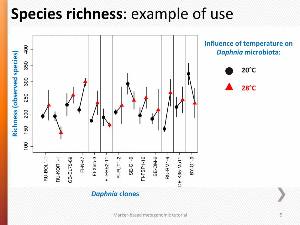
Species richness: example of use
Daphnia clones
Richne
ss (o
bserved species) Influence of temperature on
Daphnia microbiota:
20°C
28°C
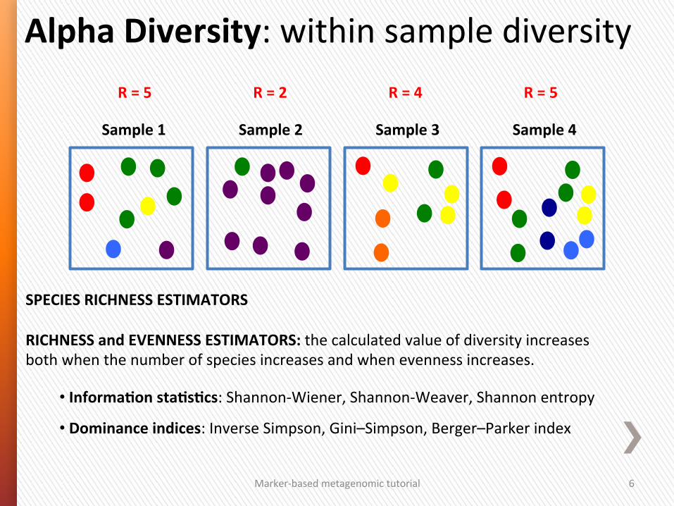
SPECIES RICHNESS ESTIMATORS RICHNESS and EVENNESS ESTIMATORS: the calculated value of diversity increases both when the number of species increases and when evenness increases.
• InformaSon staSsScs: Shannon-‐Wiener, Shannon-‐Weaver, Shannon entropy
• Dominance indices: Inverse Simpson, Gini–Simpson, Berger–Parker index
Alpha Diversity: within sample diversity
Marker-‐based metagenomic tutorial 6
Sample 1 Sample 3 Sample 4
R = 5
Sample 2
R = 2 R = 4 R = 5
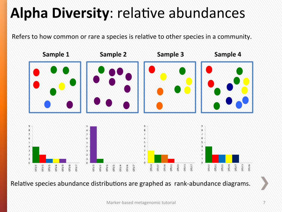
Refers to how common or rare a species is relaGve to other species in a community.
Alpha Diversity: relaGve abundances
Marker-‐based metagenomic tutorial 7
Sample 1 Sample 3 Sample 4 Sample 2
RelaGve species abundance distribuGons are graphed as rank-‐abundance diagrams.
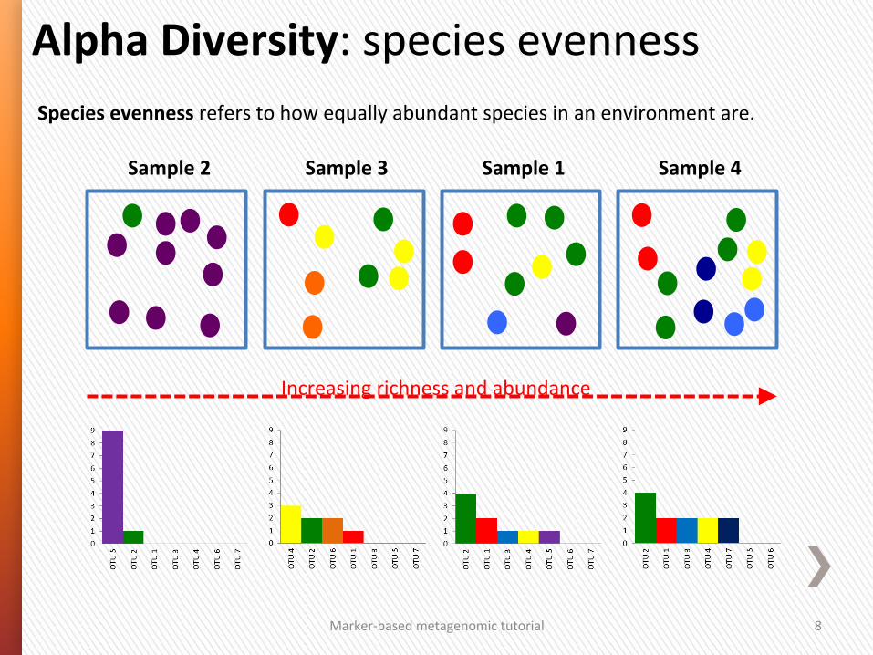
Alpha Diversity: species evenness
Marker-‐based metagenomic tutorial 8
Species evenness refers to how equally abundant species in an environment are.
Increasing richness and abundance
Sample 1 Sample 2 Sample 3 Sample 4
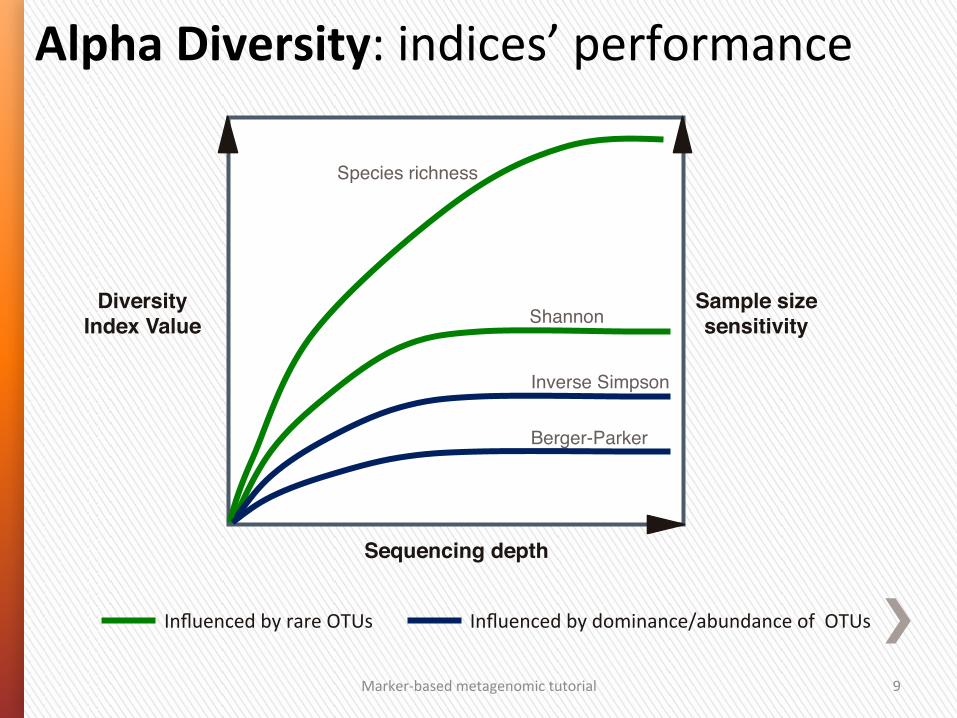
Alpha Diversity: indices’ performance
Sample size sensitivity!
Influenced by rare OTUs Influenced by dominance/abundance of OTUs
Marker-‐based metagenomic tutorial 9
Shannon"
Species richness"
Diversity Index Value!
Inverse Simpson"
Berger-Parker"
Sequencing depth!
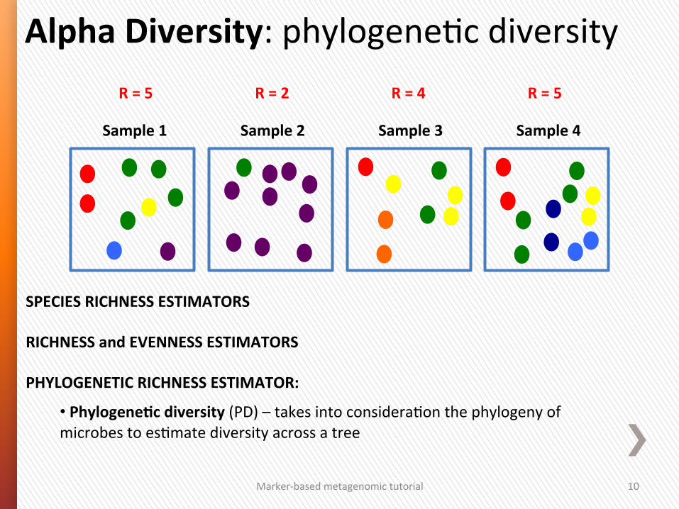
SPECIES RICHNESS ESTIMATORS RICHNESS and EVENNESS ESTIMATORS PHYLOGENETIC RICHNESS ESTIMATOR:
• PhylogeneSc diversity (PD) – takes into consideraGon the phylogeny of microbes to esGmate diversity across a tree
Alpha Diversity: phylogeneGc diversity
Marker-‐based metagenomic tutorial 10
R = 5
Sample 1 Sample 3 Sample 4 Sample 2
R = 2 R = 4 R = 5
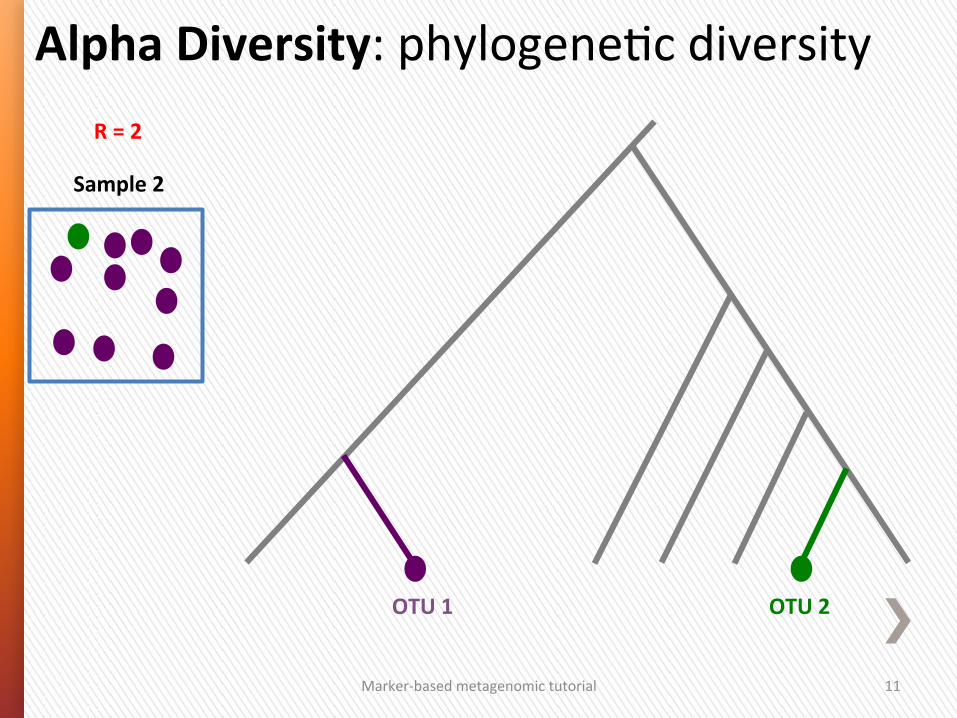
Marker-‐based metagenomic tutorial 11
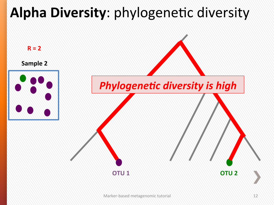
Alpha Diversity: phylogeneGc diversity
Sample 2
R = 2
OTU 2 OTU 1
Marker-‐based metagenomic tutorial 12
Alpha Diversity: phylogeneGc diversity
Sample 2
R = 2
OTU 2 OTU 1
Phylogene/c diversity is high
Marker-‐based metagenomic tutorial 13
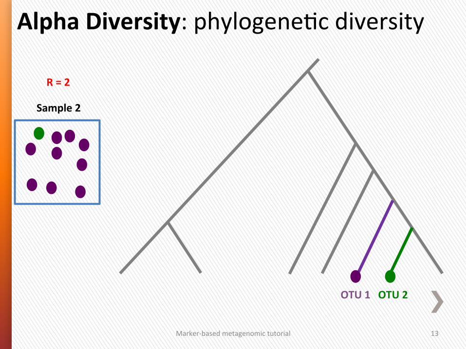
Alpha Diversity: phylogeneGc diversity
Sample 2
R = 2
OTU 2 OTU 1
Marker-‐based metagenomic tutorial 14
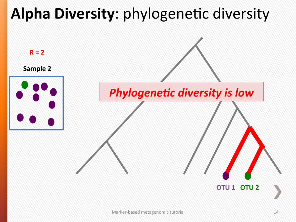
Alpha Diversity: phylogeneGc diversity
Sample 2
R = 2
OTU 2 OTU 1
Phylogene/c diversity is low

» What you want to know determines how you analyze your data
» How important is each aspect of diversity? ˃ Richness? ˃ Evenness? ˃ Dominance? ˃ Abundance? ˃ Per-‐species (relaGve) abundance? ˃ Taxon diversity?
Marker-‐based metagenomic tutorial 15
VariaGon among samples
Marker-‐based metagenomic tutorial 16
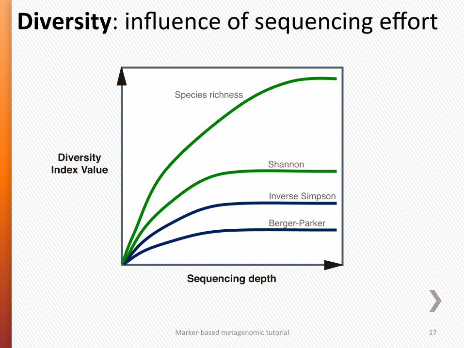
Shannon"
Species richness"
Diversity Index Value!
Inverse Simpson"
Berger-Parker"
Sequencing depth!
Diversity: influence of sequencing effort
Marker-‐based metagenomic tutorial 17
Marker-‐based metagenomic tutorial 18
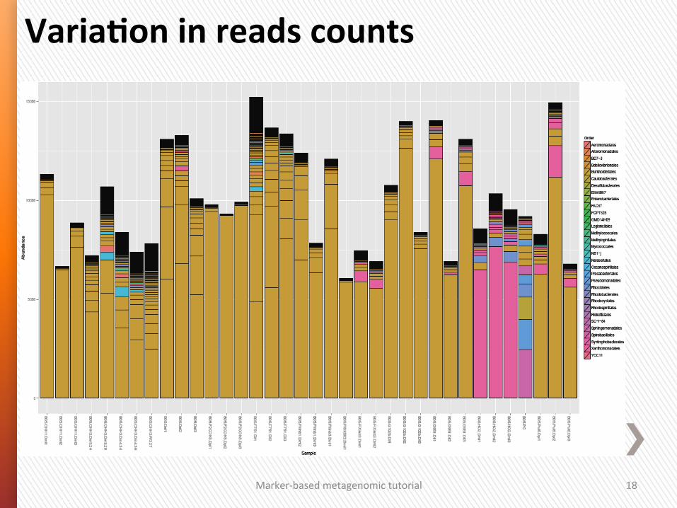
VariaSon in reads counts
Sample Addition Sequence!R
ichn
ess!
Samples: Accumulation"
Samples: Rarefaction"
Taxa: Accumulation" Taxa: Rarefaction"
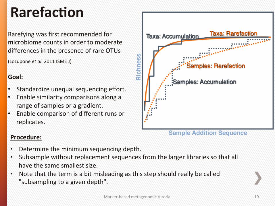
RarefacSon
Marker-‐based metagenomic tutorial 19
Rarefying was first recommended for microbiome counts in order to moderate differences in the presence of rare OTUs
(Lozupone et al. 2011 ISME J) Goal:
• Standardize unequal sequencing effort. • Enable similarity comparisons along a
range of samples or a gradient. • Enable comparison of different runs or
replicates.
Procedure:
• Determine the minimum sequencing depth. • Subsample without replacement sequences from the larger libraries so that all
have the same smallest size. • Note that the term is a bit misleading as this step should really be called
"subsampling to a given depth".
Marker-‐based metagenomic tutorial 20
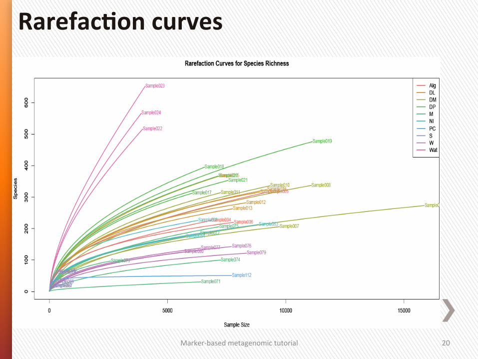
RarefacSon curves
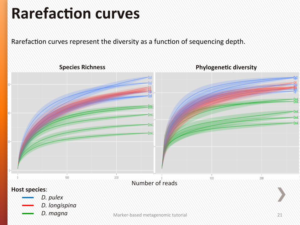
RarefacGon curves represent the diversity as a funcGon of sequencing depth.
Marker-‐based metagenomic tutorial 21
RarefacSon curves
Number of reads
Species Richness PhylogeneSc diversity
Host species: D. pulex D. longispina D. magna
RarefacSon
Marker-‐based metagenomic tutorial 22
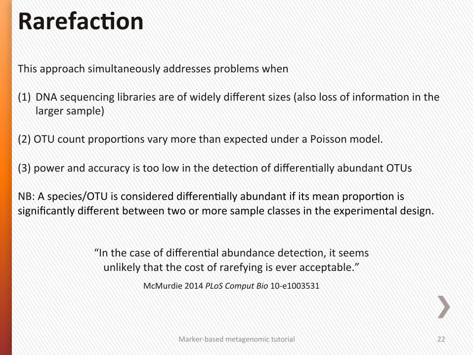
This approach simultaneously addresses problems when (1) DNA sequencing libraries are of widely different sizes (also loss of informaGon in the
larger sample) (2) OTU count proporGons vary more than expected under a Poisson model. (3) power and accuracy is too low in the detecGon of differenGally abundant OTUs NB: A species/OTU is considered differenGally abundant if its mean proporGon is significantly different between two or more sample classes in the experimental design.
“In the case of differenGal abundance detecGon, it seems unlikely that the cost of rarefying is ever acceptable.”
McMurdie 2014 PLoS Comput Bio 10-‐e1003531
AlternaSves to rarefacSon
Marker-‐based metagenomic tutorial 23
All that is leX aXer rarefacSon is the expected number of species per sample, not a real value or real data. DisGncGon between subsampling curves and normalizaGon. Randomly select evenly-‐sized samples from the larger sample • Could be done iteraGvely to provide a normalized distribuGon of the expected
number of species • Akin to the Jackknife value
Kempton & Wedderburn (1978) • Produce equal sized samples aoer fipng species abundances to gamma
distribuGon • Not commonly used Procedure: use normalizaSon tools or transform count data (e.g. use a log2(x + 1) transformaGon on count data to miGgate the impact of 0 and very high counts).
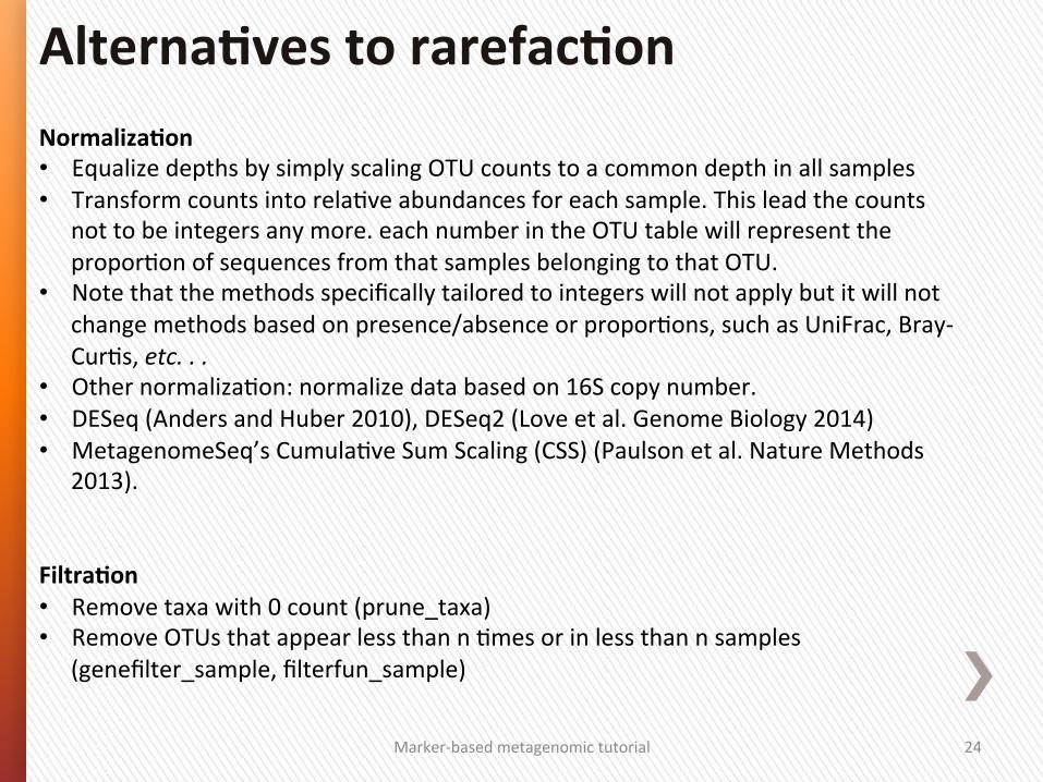
NormalizaSon • Equalize depths by simply scaling OTU counts to a common depth in all samples • Transform counts into relaGve abundances for each sample. This lead the counts
not to be integers any more. each number in the OTU table will represent the proporGon of sequences from that samples belonging to that OTU.
• Note that the methods specifically tailored to integers will not apply but it will not change methods based on presence/absence or proporGons, such as UniFrac, Bray-‐CurGs, etc. . .
• Other normalizaGon: normalize data based on 16S copy number. • DESeq (Anders and Huber 2010), DESeq2 (Love et al. Genome Biology 2014) • MetagenomeSeq’s CumulaGve Sum Scaling (CSS) (Paulson et al. Nature Methods
2013).
FiltraSon • Remove taxa with 0 count (prune_taxa) • Remove OTUs that appear less than n Gmes or in less than n samples
(genefilter_sample, filterfun_sample)
Marker-‐based metagenomic tutorial 24
AlternaSves to rarefacSon
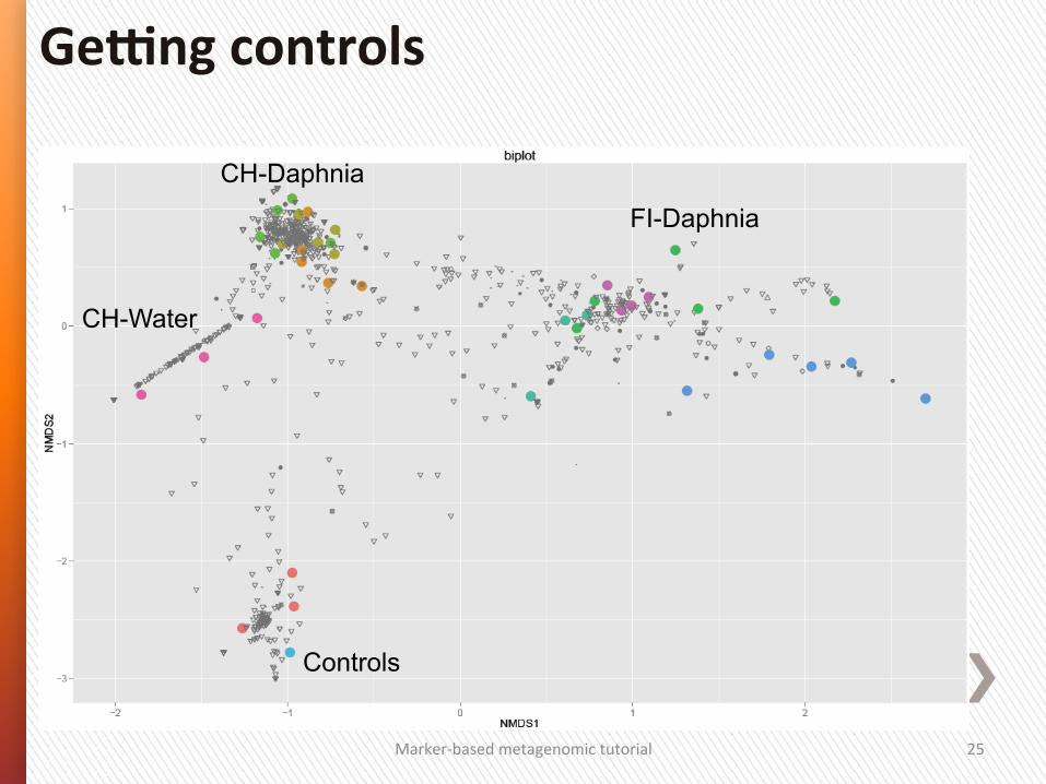
CH-Daphnia
CH-Water
Controls
FI-Daphnia
Marker-‐based metagenomic tutorial 25
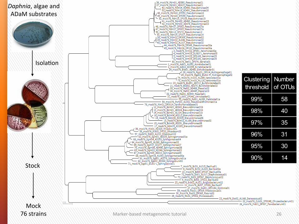
Ge]ng controls
Marker-‐based metagenomic tutorial 26
Stock
IsolaGon
Daphnia, algae and ADaM substrates
76 sequences x max.607 nuc
Mock 76 strains
Clustering threshold
Number of OTUs
99% 58
98% 40
97% 35
96% 31
95% 30
90% 14
β-‐diversity metrics
Marker-‐based metagenomic tutorial 27
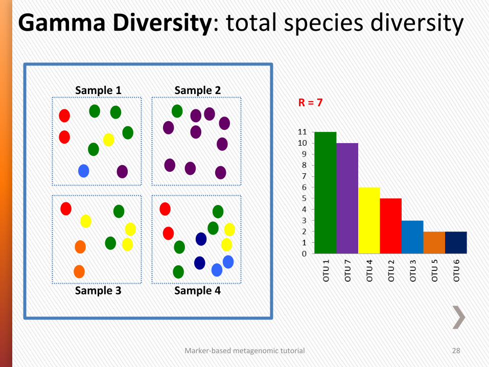
Gamma Diversity: total species diversity
Marker-‐based metagenomic tutorial 28
Sample 1 Sample 2
Sample 3 Sample 4
R = 7
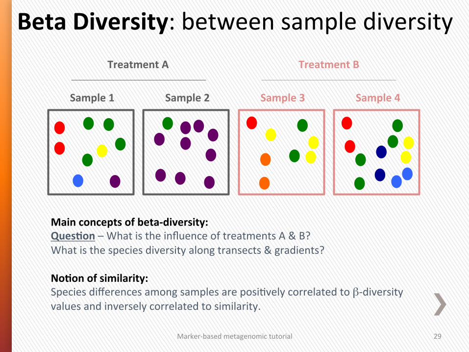
Main concepts of beta-‐diversity: QuesSon – What is the influence of treatments A & B? What is the species diversity along transects & gradients? NoSon of similarity: Species differences among samples are posiGvely correlated to β-‐diversity values and inversely correlated to similarity.
Marker-‐based metagenomic tutorial 29
Beta Diversity: between sample diversity
Sample 3 Sample 4 Sample 1 Sample 2
Treatment A Treatment B
Marker-‐based metagenomic tutorial 30
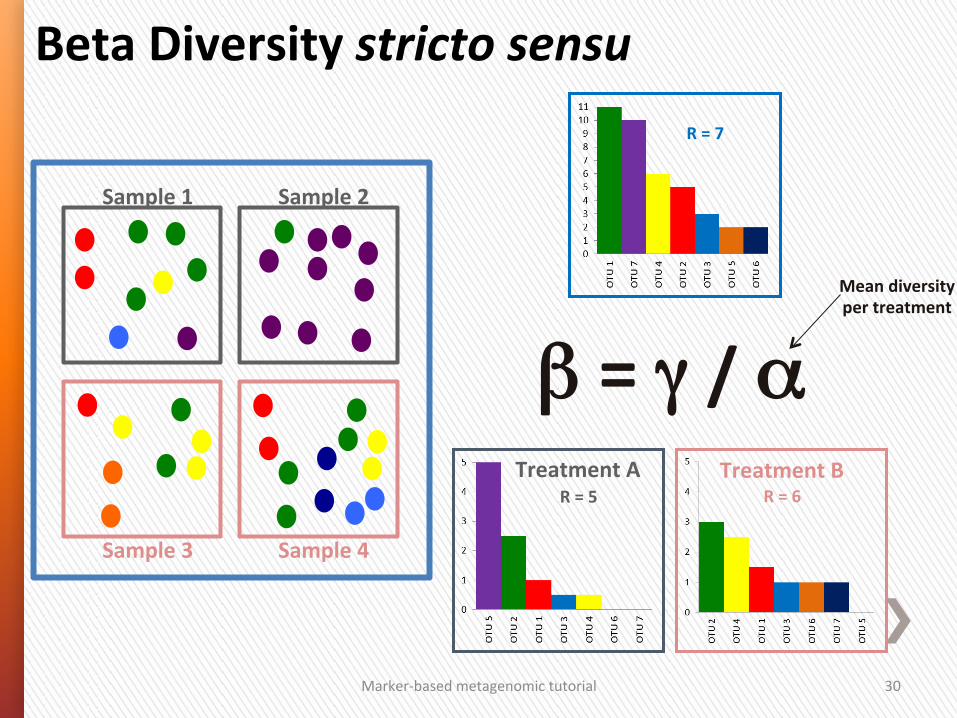
R = 7
Sample 1 Sample 2
Sample 3 Sample 4
β = γ / α R = 5
Treatment A R = 6
Treatment B
Beta Diversity stricto sensu
Mean diversity per treatment
Marker-‐based metagenomic tutorial 31
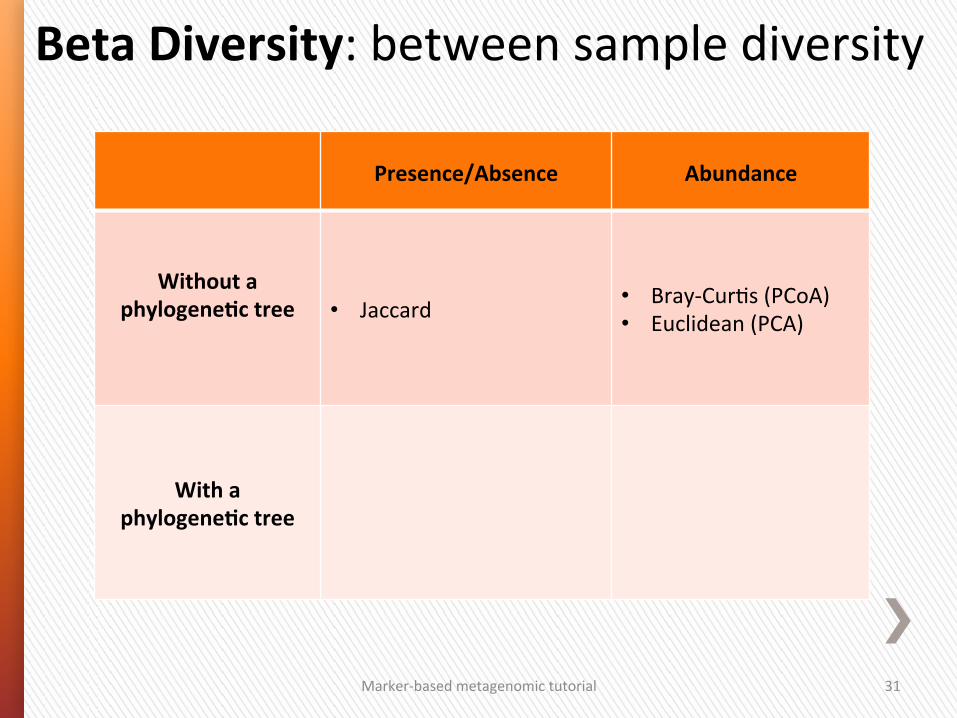
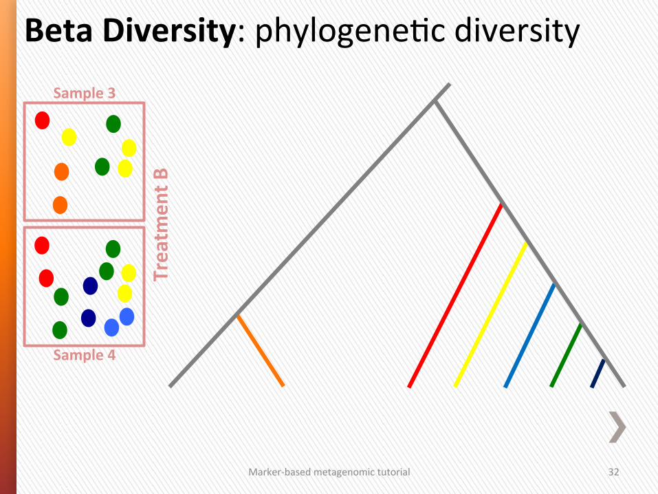
Beta Diversity: between sample diversity
Presence/Absence Abundance
Without a phylogeneSc tree
• Jaccard • Bray-‐CurGs (PCoA)
• Euclidean (PCA)
With a phylogeneSc tree
Marker-‐based metagenomic tutorial 32
Beta Diversity: phylogeneGc diversity Sample 3
Sample 4
Treatm
ent B
Marker-‐based metagenomic tutorial 33
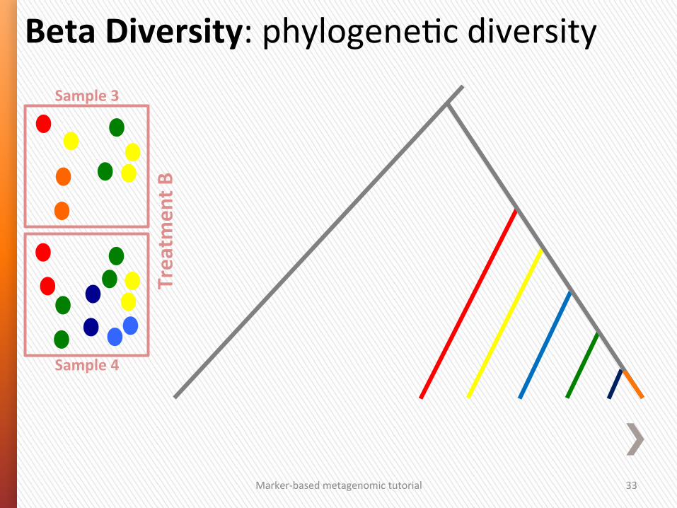
Beta Diversity: phylogeneGc diversity Sample 3
Sample 4
Treatm
ent B
Marker-‐based metagenomic tutorial 34
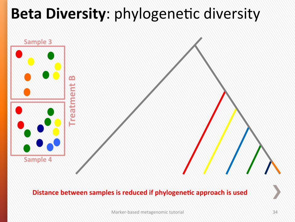
Beta Diversity: phylogeneGc diversity Sample 3
Sample 4
Treatm
ent B
Distance between samples is reduced if phylogeneSc approach is used
Marker-‐based metagenomic tutorial 35
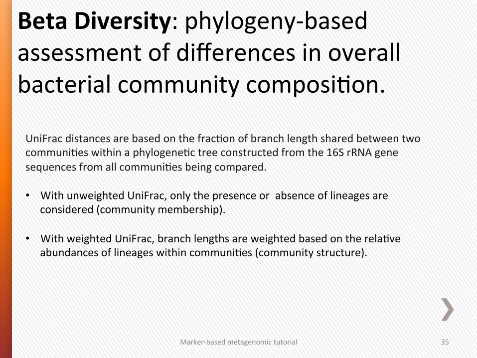
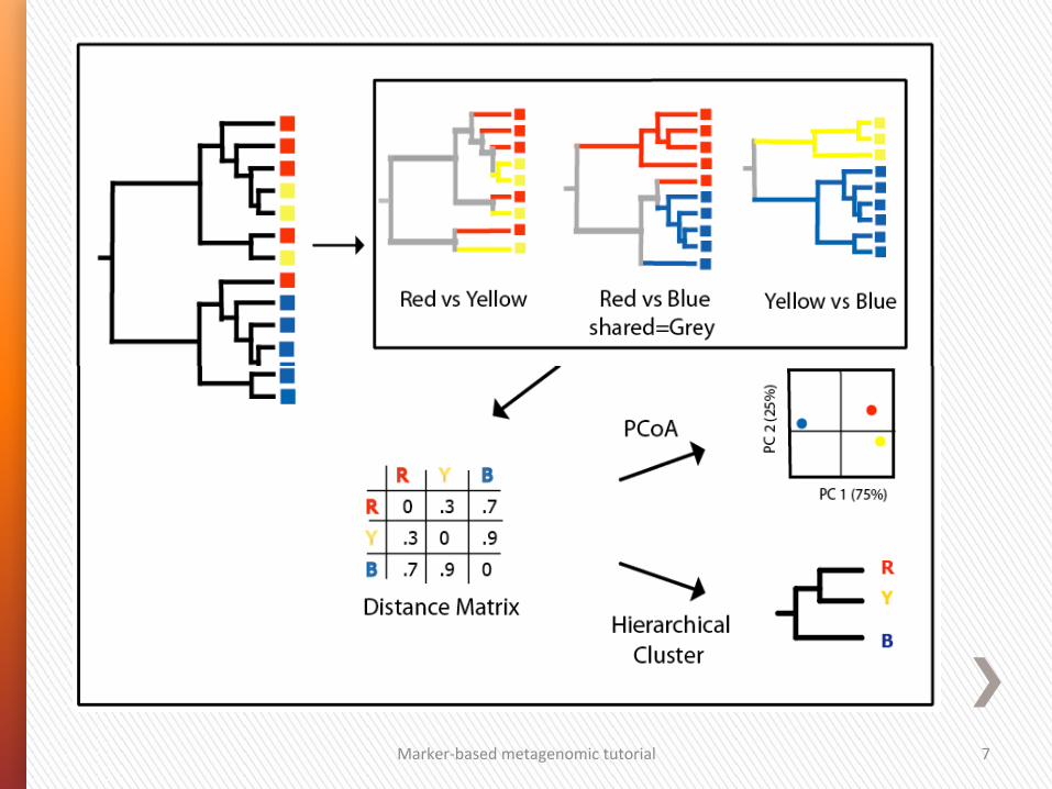
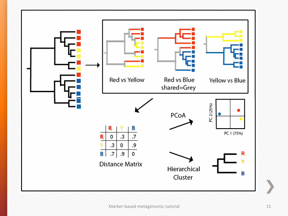
Beta Diversity: phylogeny-‐based assessment of differences in overall bacterial community composiGon.
UniFrac distances are based on the fracGon of branch length shared between two communiGes within a phylogeneGc tree constructed from the 16S rRNA gene sequences from all communiGes being compared.
• With unweighted UniFrac, only the presence or absence of lineages are considered (community membership).
• With weighted UniFrac, branch lengths are weighted based on the relaGve abundances of lineages within communiGes (community structure).
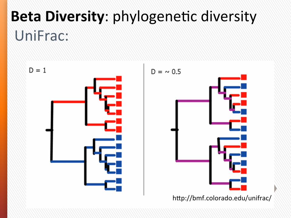
Measuring$Microbial$Communi+es:$UniFrac$Metric$
hep://bmf.colorado.edu/unifrac/$
Used$to$analyzed$shared$branch$length$of$mul+ple$microbial$communi+es$
Beta Diversity: phylogeneGc diversity UniFrac:
Marker-‐based metagenomic tutorial 37
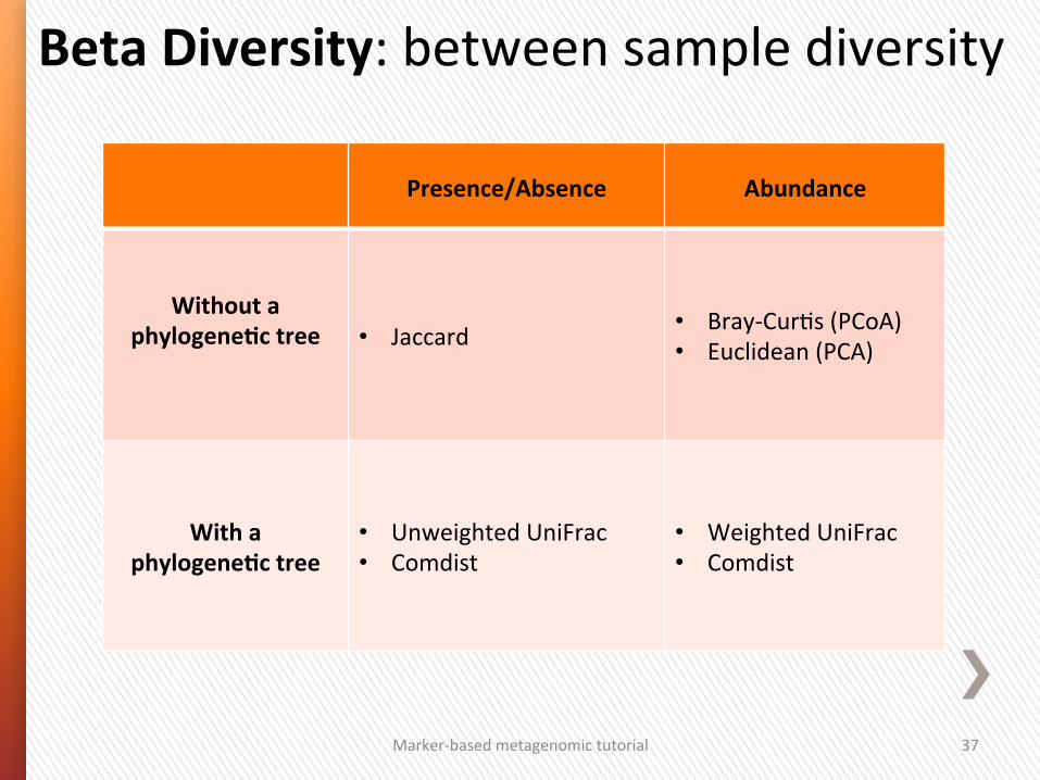
Beta Diversity: between sample diversity
Presence/Absence Abundance
Without a phylogeneSc tree
• Jaccard • Bray-‐CurGs (PCoA)
• Euclidean (PCA)
With a phylogeneSc tree
• Unweighted UniFrac • Comdist
• Weighted UniFrac • Comdist
38
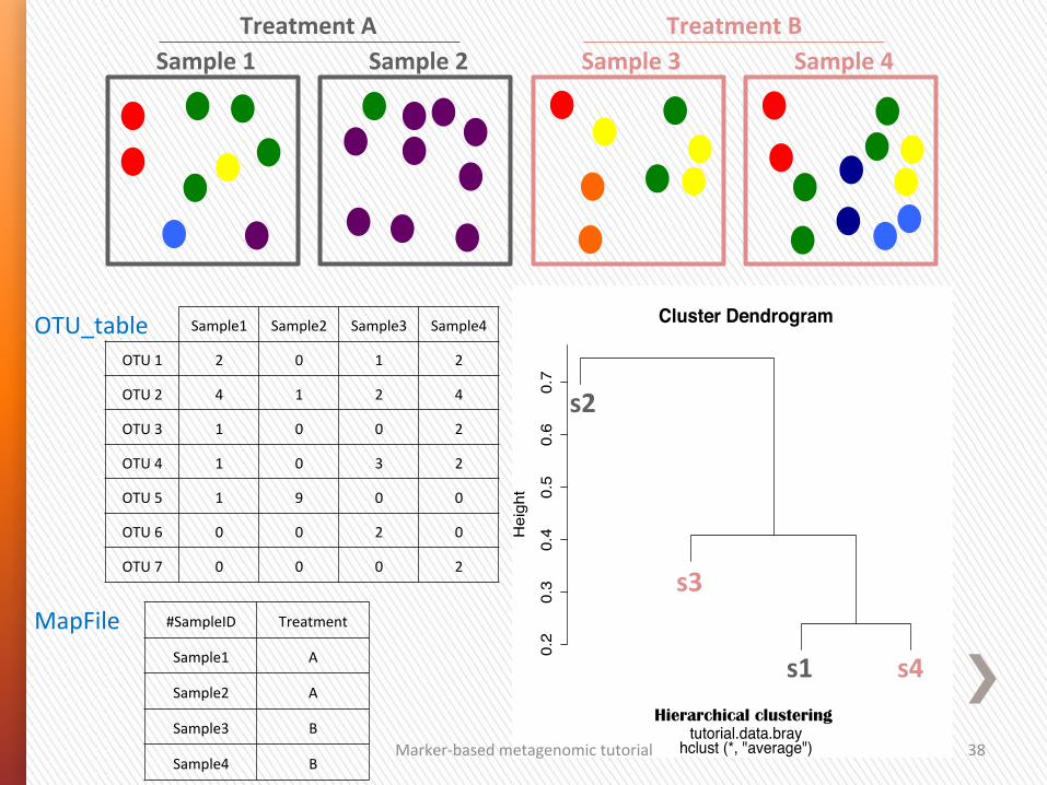
2
3
1 4
0.2
0.3
0.4
0.5
0.6
0.7
Cluster Dendrogram
hclust (*, "average")tutorial.data.bray
Hei
ght
s4
s3
s1
s2
Hierarchical clustering
Sample1 Sample2 Sample3 Sample4
OTU 1 2 0 1 2
OTU 2 4 1 2 4
OTU 3 1 0 0 2
OTU 4 1 0 3 2
OTU 5 1 9 0 0
OTU 6 0 0 2 0
OTU 7 0 0 0 2
#SampleID Treatment
Sample1 A
Sample2 A
Sample3 B
Sample4 B
Sample 3 Sample 4 Sample 1 Sample 2 Treatment A Treatment B
Marker-‐based metagenomic tutorial
OTU_table
MapFile
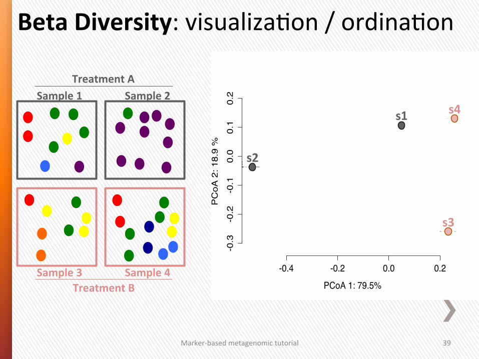
Marker-‐based metagenomic tutorial 39
-0.4 -0.2 0.0 0.2
-0.3
-0.2
-0.1
0.0
0.1
0.2
PCoA 1: 79.5%
PC
oA 2
: 18.
9 %
site1
site2
site3
site4s4
s2
s1
s3
Beta Diversity: visualizaGon / ordinaGon
Sample 1 Sample 2
Sample 3 Sample 4
Treatment A
Treatment B
» What you want to know determines how you analyze your data
» How important is each aspect of diversity? ˃ Richness? ˃ Evenness? ˃ Dominance? ˃ Abundance? ˃ Per-‐species (relaGve) abundance? ˃ Taxon diversity?
Marker-‐based metagenomic tutorial 40
Comparison of samples or group of samples:
How similar are communi4es?
Marker-‐based metagenomic tutorial 1
Marker-‐based metagenomic tutorial 2
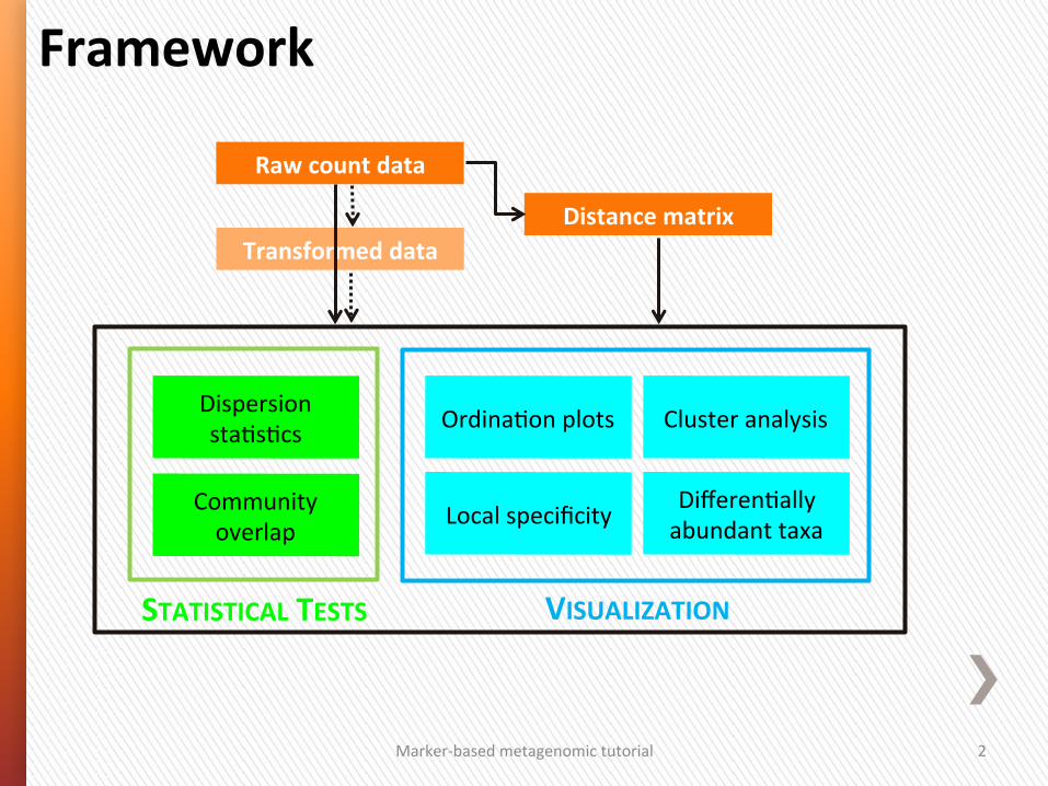
Local specificity Community overlap
Dispersion sta4s4cs
VISUALIZATION
Differen4ally abundant taxa
Ordina4on plots Cluster analysis
Framework
Raw count data
Distance matrix Transformed data
STATISTICAL TESTS
Marker-‐based metagenomic tutorial 3
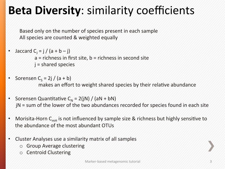
Beta Diversity: similarity coefficients Based only on the number of species present in each sample All species are counted & weighted equally
• Jaccard CJ = j / (a + b – j) a = richness in first site, b = richness in second site j = shared species
• Sorensen CS = 2j / (a + b)
makes an effort to weight shared species by their rela4ve abundance • Sorensen Quan4ta4ve CN = 2(jN) / (aN + bN) jN = sum of the lower of the two abundances recorded for species found in each site • Morisita-‐Horn CmH is not influenced by sample size & richness but highly sensi4ve to
the abundance of the most abundant OTUs
• Cluster Analyses use a similarity matrix of all samples o Group Average clustering o Centroid Clustering
Marker-‐based metagenomic tutorial 4
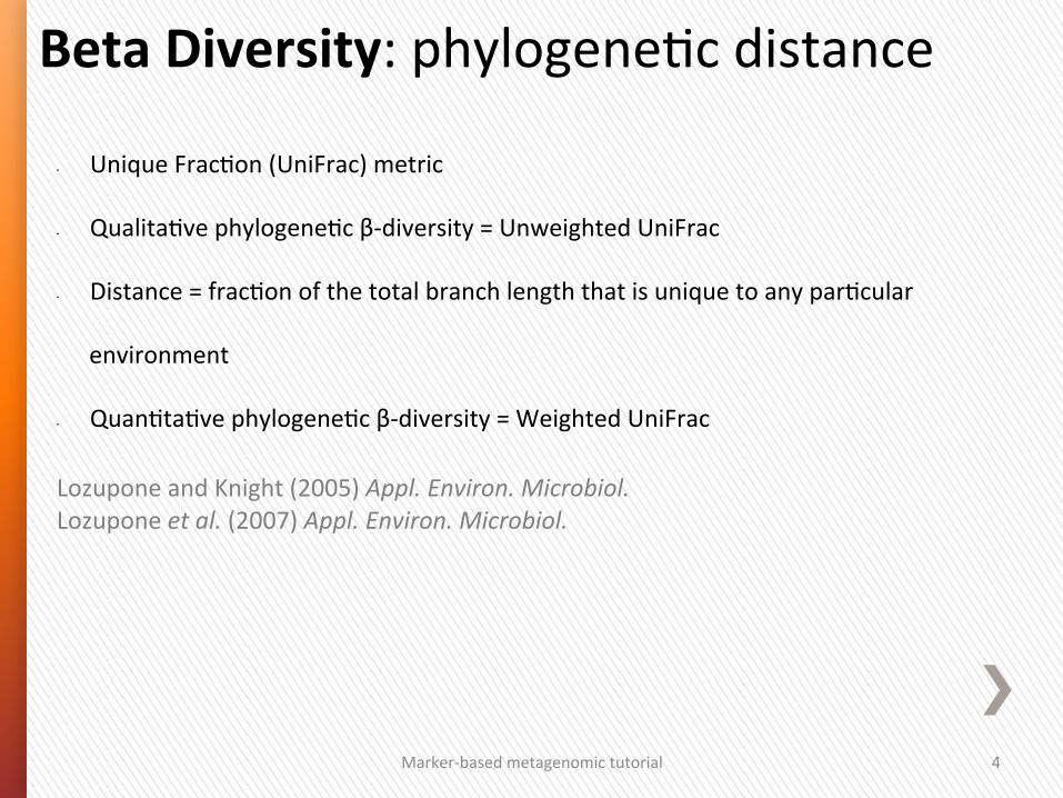
Beta Diversity: phylogene4c distance
• Unique Frac4on (UniFrac) metric
• Qualita4ve phylogene4c β-‐diversity = Unweighted UniFrac
• Distance = frac4on of the total branch length that is unique to any par4cular
environment
• Quan4ta4ve phylogene4c β-‐diversity = Weighted UniFrac Lozupone and Knight (2005) Appl. Environ. Microbiol. Lozupone et al. (2007) Appl. Environ. Microbiol.
Marker-‐based metagenomic tutorial 5
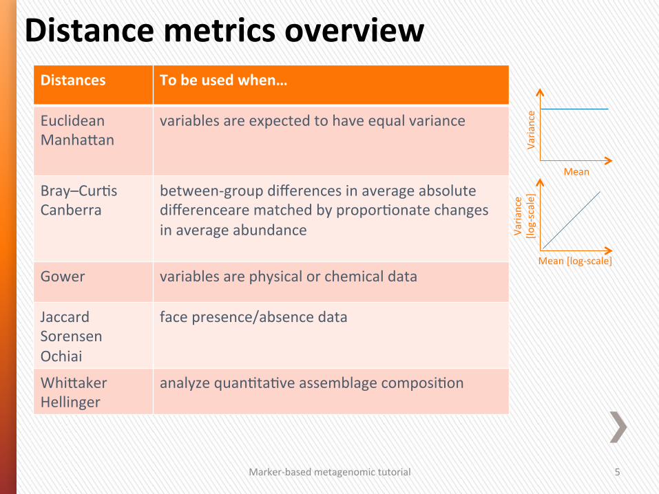
Distances To be used when…
Euclidean Manhagan
variables are expected to have equal variance
Bray–Cur4s Canberra
between-‐group differences in average absolute differenceare matched by propor4onate changes in average abundance
Gower variables are physical or chemical data
Jaccard Sorensen Ochiai
face presence/absence data
Whigaker Hellinger
analyze quan4ta4ve assemblage composi4on
Mean
Varia
nce
Mean [log-‐scale]
Varia
nce
[log-‐scale]
Distance metrics overview

Marker-‐based metagenomic tutorial 6
Local specificity Community overlap
Dispersion sta4s4cs
VISUALIZATION
Differen4ally abundant taxa
Ordina4on plots Cluster analysis
Framework
Raw count data
Distance matrix Transformed data
STATISTICAL TESTS
Marker-‐based metagenomic tutorial 7
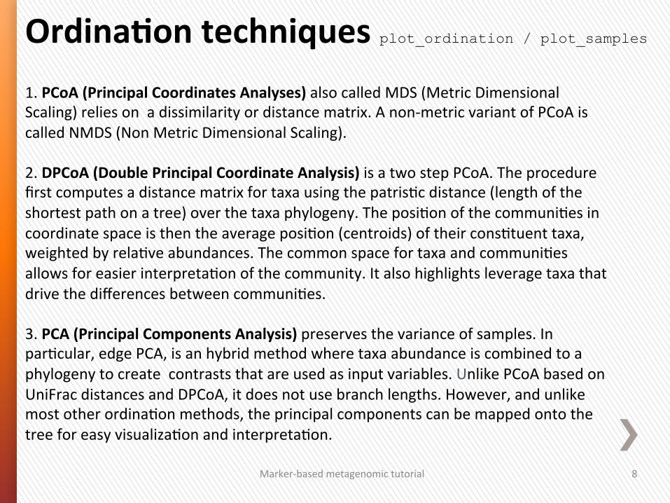
OrdinaGon techniques plot_ordination / plot_samples 1. PCoA (Principal Coordinates Analyses) also called MDS (Metric Dimensional Scaling) relies on a dissimilarity or distance matrix. A non-‐metric variant of PCoA is called NMDS (Non Metric Dimensional Scaling). 2. DPCoA (Double Principal Coordinate Analysis) is a two step PCoA. The procedure first computes a distance matrix for taxa using the patris4c distance (length of the shortest path on a tree) over the taxa phylogeny. The posi4on of the communi4es in coordinate space is then the average posi4on (centroids) of their cons4tuent taxa, weighted by rela4ve abundances. The common space for taxa and communi4es allows for easier interpreta4on of the community. It also highlights leverage taxa that drive the differences between communi4es. 3. PCA (Principal Components Analysis) preserves the variance of samples. In par4cular, edge PCA, is an hybrid method where taxa abundance is combined to a phylogeny to create contrasts that are used as input variables. Unlike PCoA based on UniFrac distances and DPCoA, it does not use branch lengths. However, and unlike most other ordina4on methods, the principal components can be mapped onto the tree for easy visualiza4on and interpreta4on.
Marker-‐based metagenomic tutorial 8
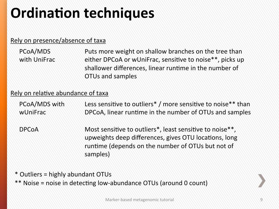
DPCoA
PCoA/MDS with wUniFrac
PCoA/MDS with UniFrac
Most sensi4ve to outliers*, least sensi4ve to noise**, upweights deep differences, gives OTU loca4ons, long run4me (depends on the number of OTUs but not of samples)
* Outliers = highly abundant OTUs ** Noise = noise in detec4ng low-‐abundance OTUs (around 0 count)
Less sensi4ve to outliers* / more sensi4ve to noise** than DPCoA, linear run4me in the number of OTUs and samples
Puts more weight on shallow branches on the tree than either DPCoA or wUniFrac, sensi4ve to noise**, picks up shallower differences, linear run4me in the number of OTUs and samples
Rely on rela4ve abundance of taxa
Rely on presence/absence of taxa
Marker-‐based metagenomic tutorial 9
OrdinaGon techniques
Linear
Unimodal
Marker-‐based metagenomic tutorial 10
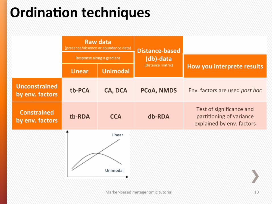
OrdinaGon techniques
Raw data (presence/absence or abundance data) Distance-‐based
(db)-‐data (distance matrix)
Response along a gradient
How you interprete results Linear Unimodal
Unconstrained by env. factors tb-‐PCA CA, DCA PCoA, NMDS Env. factors are used post hoc
Constrained by env. factors tb-‐RDA CCA db-‐RDA
Test of significance and par44oning of variance explained by env. factors
Marker-‐based metagenomic tutorial 11
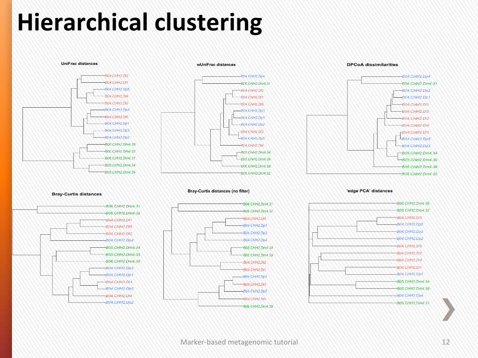
Hierarchical clustering
Marker-‐based metagenomic tutorial 12
1. Use a distance measure that is ecologically meaningful. A good analysis prac4ce is to repeat the analysis with several good distance measures and inves4gate whether all these analyses lead to the same conclusion.
2. Inves4gate how well the distances in the ordina4on graph represent the total distances (e.g.
Marker-‐based metagenomic tutorial 13
Distance-‐based analyses

Marker-‐based metagenomic tutorial 14
Local specificity Community overlap
Dispersion sta4s4cs
VISUALIZATION
Differen4ally abundant taxa
Ordina4on plots Cluster analysis
Framework
Raw count data
Distance matrix Transformed data
STATISTICAL TESTS
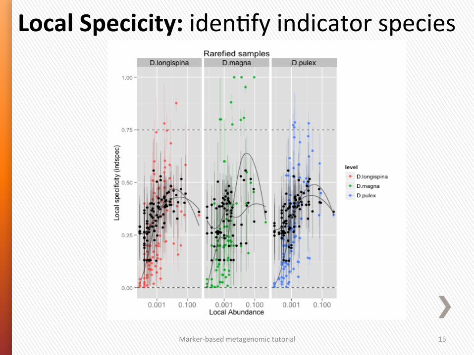
Local Specicity: iden4fy indicator species
Marker-‐based metagenomic tutorial 15
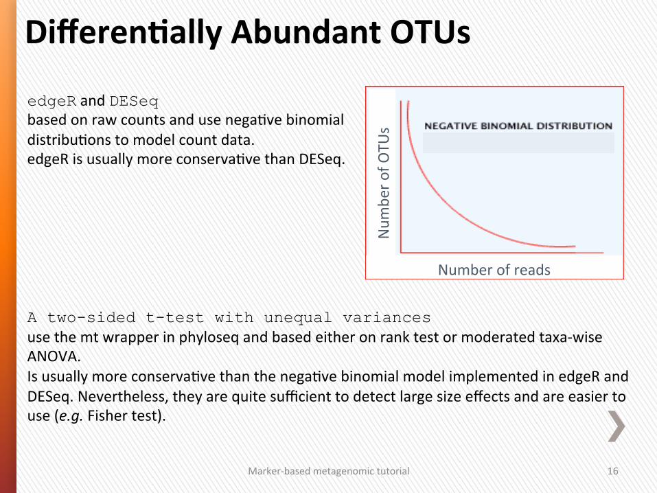
edgeR and DESeq based on raw counts and use nega4ve binomial distribu4ons to model count data. edgeR is usually more conserva4ve than DESeq. A two-sided t-test with unequal variances use the mt wrapper in phyloseq and based either on rank test or moderated taxa-‐wise ANOVA. Is usually more conserva4ve than the nega4ve binomial model implemented in edgeR and DESeq. Nevertheless, they are quite sufficient to detect large size effects and are easier to use (e.g. Fisher test).
Marker-‐based metagenomic tutorial 16
DifferenGally Abundant OTUs
Number of reads
Num
ber o
f OTU
s
StaGsGcal tests for different membership • UniFrac Significance: frac4on of random trees that have more Unique branch
length than the real tree.
• Phylogene4c (P) Test: based on the number of changes between states (samples) required to explain the distribu4on of sequences on the tree (Fitch parsimony). Sensi4ve to tree topology but not to branch lengths. See Mar4n AP (2002) Appl. Environ. Microbiol.
• LibShuff
Marker-‐based metagenomic tutorial 17
Marker-‐based metagenomic tutorial 18
The libshuff method is a generic test that describes whether two or more communi4es have the same structure using the Cramer-‐von Mises test sta4s4c. The significance of the sta4s4cal test indicates the probability that the communi4es have the same structure by chance. Because each pairwise comparison requires two significance tests, a correc4on for mul4ple comparisons (e.g. Bonferroni's correc4on) must be applied. The program calculates a homologous and a heterologous coverage curve for the libraries then calculates the distance between the two curves and use a Monte Carlo test procedure to compare them. NB: Monte Carlo simula4ons: randomly permute the data (environment assignments) and determine how oten the random data has a more extreme value than the real data. Singleton DR et al. (2001) Appl. Environ. Microbiol. Schloss PD et al. (2004) Appl. Environ. Microbiol. hgps://toolshed.g2.bx.psu.edu/repos/jjohnson/mothur_toolsuite
Libshuff (Library shuffling)
StaGsGcal tests for different membership • UniFrac Significance: frac4on of random trees that have more Unique branch
length than the real tree.
• Phylogene4c (P) Test: based on the number of changes between states (samples) required to explain the distribu4on of sequences on the tree (Fitch parsimony). Sensi4ve to tree topology but not to branch lengths. See Mar4n AP (2002) Appl. Environ. Microbiol.
• LibShuff
• ADONIS: Analysis of variance using distance matrices (vegan package in R). formal tes4ng of sample covariates is also done using a permuta4on MANOVA with the (squared) distances and covariates as response and linear predictors, respec4vely. See Anderson (2001) Austral Ecology
• ANOSIM
• Mantel test
Note that these mul4variate analyses can be heavily influenced by heterogeneity of dispersion across groups in an unbalanced design. See Anderson and Walsh (2013) Ecological Monographs
Marker-‐based metagenomic tutorial 19
Dispersion • Dispersion is defined as a change in mean–variance rela4onship
• Permuta4on test of homogeneity of group dispersion. It is an analogue to homogeneity of variances.
• Test if all groups share a common dispersion (i.e. if the varia4on between samples is similar to the varia4on between groups).
• Dispersion of sequences in the tree
See Webb CO (2000) American Naturalist
Marker-‐based metagenomic tutorial 20