DepartmentofElectrical,Computer,andEnergyEngineering...
48
R. W. Erickson Department of Electrical, Computer, and Energy Engineering University of Colorado, Boulder
Transcript of DepartmentofElectrical,Computer,andEnergyEngineering...
R. W. Erickson Department of Electrical, Computer, and Energy Engineering
University of Colorado, Boulder
Fundamentals of Power Electronics Chapter 13: Basic Magnetics Theory35
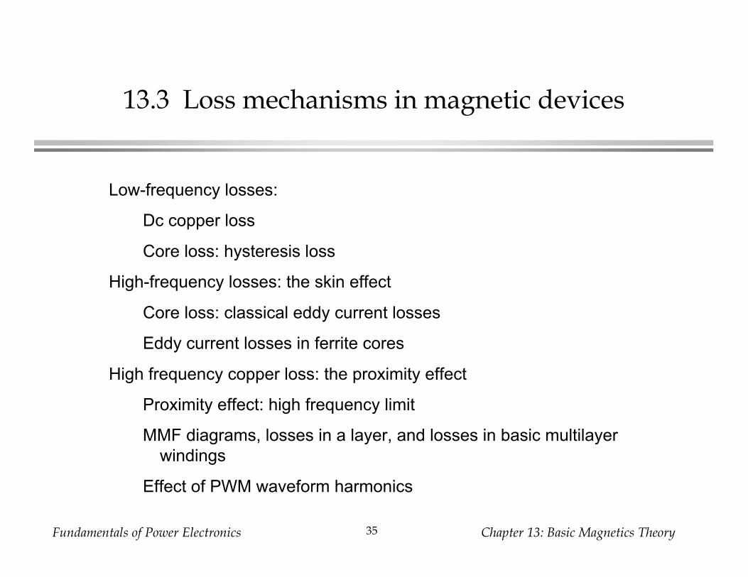
13.3 Loss mechanisms in magnetic devices
Low-frequency losses:
Dc copper loss
Core loss: hysteresis loss
High-frequency losses: the skin effect
Core loss: classical eddy current losses
Eddy current losses in ferrite cores
High frequency copper loss: the proximity effect
Proximity effect: high frequency limit
MMF diagrams, losses in a layer, and losses in basic multilayer
windings
Effect of PWM waveform harmonics
Fundamentals of Power Electronics Chapter 13: Basic Magnetics Theory36
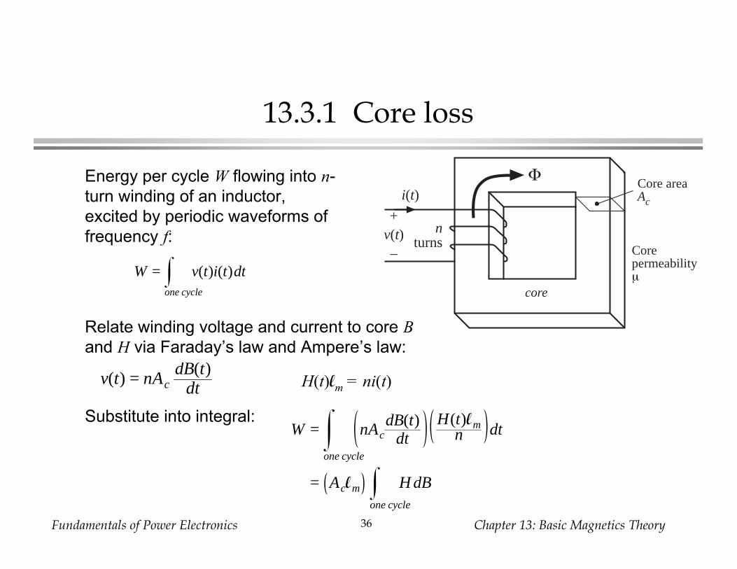
13.3.1 Core loss
Energy per cycle W flowing into n-
turn winding of an inductor,
excited by periodic waveforms of
frequency f:
Relate winding voltage and current to core B
and H via Faraday’s law and Ampere’s law:
H(t)lm = ni(t)
Substitute into integral:
core
nturns
Core areaAc
Corepermeabilityµ
+v(t)–
i(t)Φ
W = v(t)i(t)dtone cycle
v(t) = nAcdB(t)
dt
W = nAcdB(t)
dtH(t)lm
n dt
one cycle
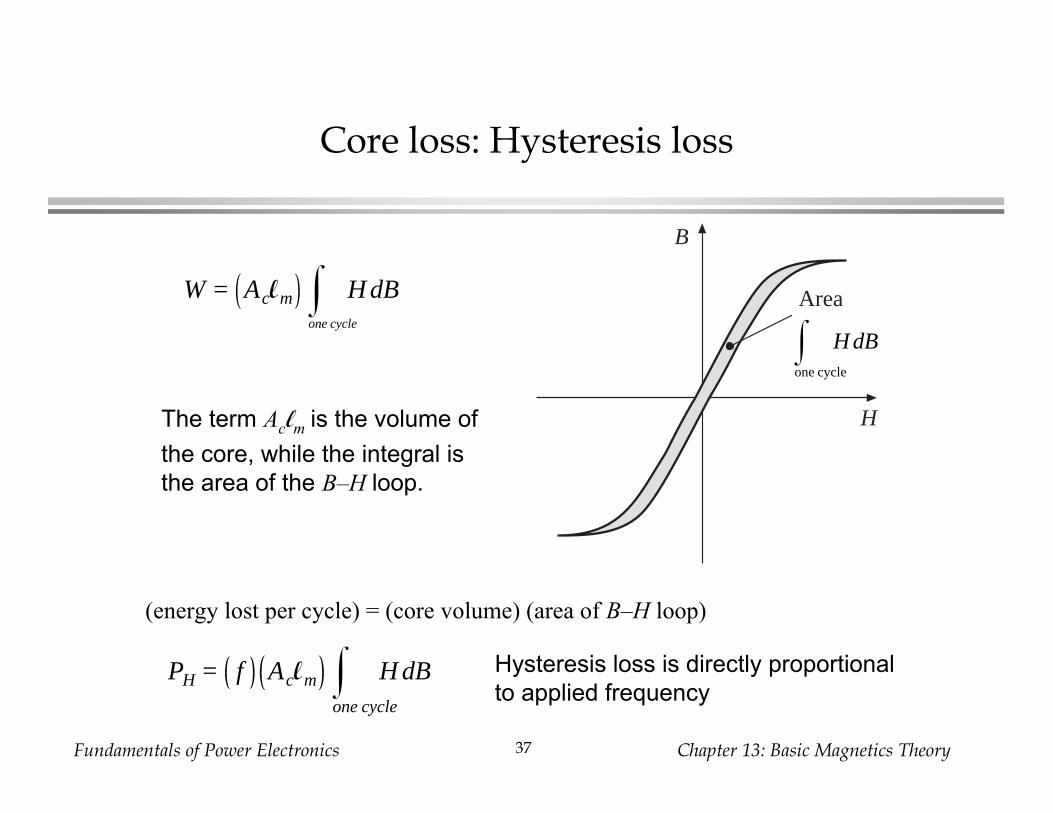
= Aclm H dBone cycle
Fundamentals of Power Electronics Chapter 13: Basic Magnetics Theory37
Core loss: Hysteresis loss
(energy lost per cycle) = (core volume) (area of B–H loop)
The term Aclm is the volume of
the core, while the integral is
the area of the B–H loop.
Hysteresis loss is directly proportional
to applied frequency
B
H
Area
H dBone cycle
W = Aclm H dBone cycle
PH = f Aclm H dBone cycle
Fundamentals of Power Electronics Chapter 13: Basic Magnetics Theory38
Modeling hysteresis loss
• Hysteresis loss varies directly with applied frequency
• Dependence on maximum flux density: how does area of B–H loop
depend on maximum flux density (and on applied waveforms)?
Empirical equation (Steinmetz equation):
The parameters KH and are determined experimentally.
Dependence of PH on Bmax is predicted by the theory of magnetic
domains.
PH = KH f Bmaxα (core volume)
Fundamentals of Power Electronics Chapter 13: Basic Magnetics Theory39
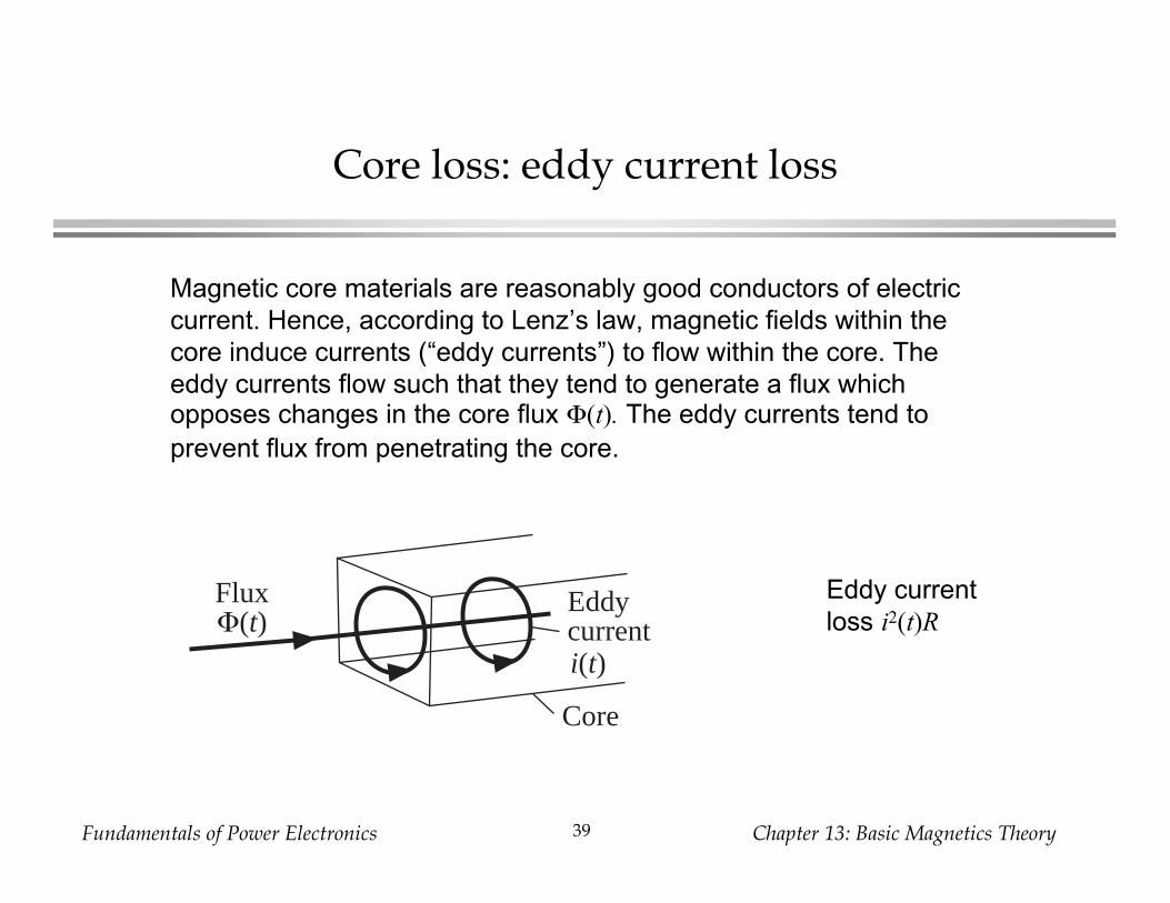
Core loss: eddy current loss
Magnetic core materials are reasonably good conductors of electric
current. Hence, according to Lenz’s law, magnetic fields within the
core induce currents (“eddy currents”) to flow within the core. The
eddy currents flow such that they tend to generate a flux whichopposes changes in the core flux (t). The eddy currents tend to
prevent flux from penetrating the core.
Eddy current
loss i2(t)RFluxΦ(t)
Core
i(t)
Eddycurrent
Fundamentals of Power Electronics Chapter 13: Basic Magnetics Theory40
Modeling eddy current loss
• Ac flux (t) induces voltage v(t) in core, according to Faraday’s law.
Induced voltage is proportional to derivative of (t). In
consequence, magnitude of induced voltage is directly proportional
to excitation frequency f.
• If core material impedance Z is purely resistive and independent of
frequency, Z = R, then eddy current magnitude is proportional to
voltage: i(t) = v(t)/R. Hence magnitude of i(t) is directly proportional
to excitation frequency f.
• Eddy current power loss i2(t)R then varies with square of excitation
frequency f.
• Classical Steinmetz equation for eddy current loss:
• Ferrite core material impedance is capacitive. This causes eddy
current power loss to increase as f 4.
PE = KE f 2Bmax2 (core volume)
Fundamentals of Power Electronics Chapter 13: Basic Magnetics Theory41
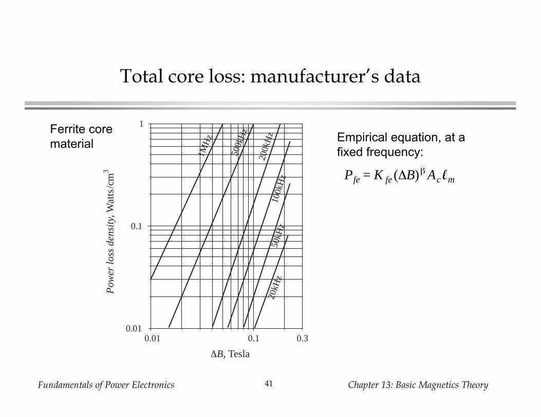
Total core loss: manufacturer’s data
Empirical equation, at a
fixed frequency:
Ferrite core
material
∆B, Tesla
0.01 0.1 0.3
Pow
er lo
ss d
ensi
ty, W
atts
/cm
3
0.01
0.1
1
20kH
z50
kHz
100k
Hz
200k
Hz
500k
Hz
1MH
z
Pfe = K fe (∆B)β Ac lm
Fundamentals of Power Electronics Chapter 13: Basic Magnetics Theory42
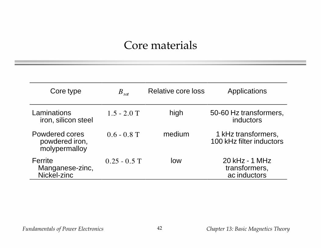
Core materials
Core type Bsat
Relative core loss Applications
Laminationsiron, silicon steel
1.5 - 2.0 T high 50-60 Hz transformers,inductors
Powdered corespowdered iron,molypermalloy
0.6 - 0.8 T medium 1 kHz transformers,100 kHz filter inductors
FerriteManganese-zinc,Nickel-zinc
0.25 - 0.5 T low 20 kHz - 1 MHztransformers,ac inductors
Fundamentals of Power Electronics Chapter 13: Basic Magnetics Theory43
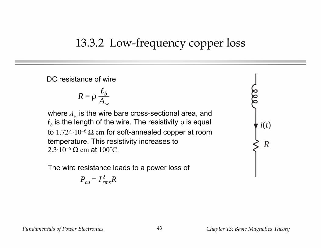
13.3.2 Low-frequency copper loss
DC resistance of wire
where Aw is the wire bare cross-sectional area, and
lb is the length of the wire. The resistivity is equal
to 1.724 10–6 cm for soft-annealed copper at room
temperature. This resistivity increases to2.3 10–6 cm at 100˚C.
The wire resistance leads to a power loss of
R
i(t)
R = ρlb
Aw
Pcu = I rms2 R
Fundamentals of Power Electronics Chapter 13: Basic Magnetics Theory44
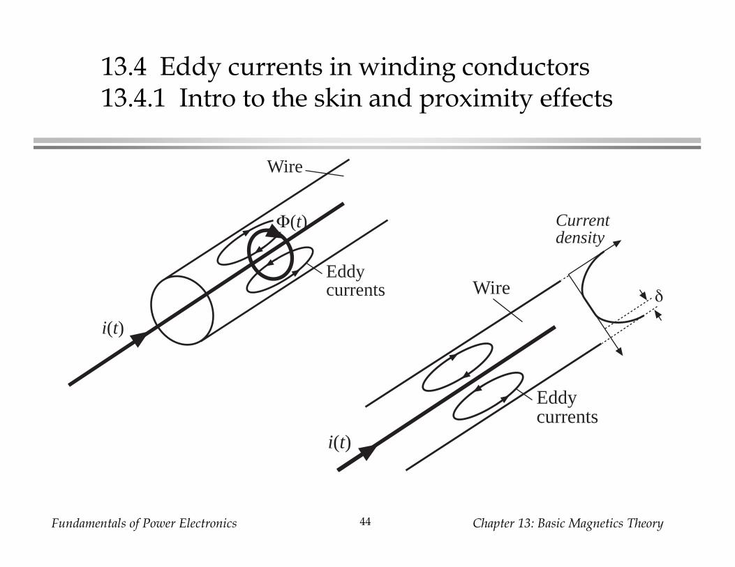
13.4 Eddy currents in winding conductors13.4.1 Intro to the skin and proximity effects
i(t)
Wire
Φ(t)
Eddycurrents
i(t)
Wire
Eddycurrents
Currentdensity
δ
Fundamentals of Power Electronics Chapter 13: Basic Magnetics Theory45
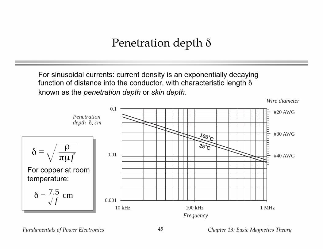
For sinusoidal currents: current density is an exponentially decayingfunction of distance into the conductor, with characteristic length
known as the penetration depth or skin depth.
Penetration depth
Frequency
100˚C25˚C
#20 AWG
Wire diameter
#30 AWG
#40 AWG
Penetrationdepth δ, cm
0.001
0.01
0.1
10 kHz 100 kHz 1 MHz
For copper at room
temperature:
δ =ρ
πµ f
δ = 7.5f
cm
Fundamentals of Power Electronics Chapter 13: Basic Magnetics Theory46
The proximity effect
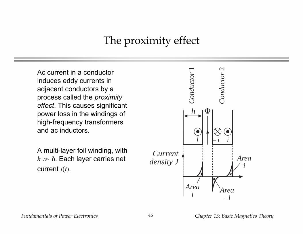
Ac current in a conductor
induces eddy currents in
adjacent conductors by a
process called the proximity
effect. This causes significant
power loss in the windings of
high-frequency transformers
and ac inductors.
A multi-layer foil winding, with
h > . Each layer carries net
current i(t).
i – i i
Currentdensity J
h Φ
Areai
Area– i
Areai
Con
duct
or 1
Con
duct
or 2
Fundamentals of Power Electronics Chapter 13: Basic Magnetics Theory47
Example: a two-winding transformer
Secondary windingPrimary winding
Core
{ {
Lay
er 1
Lay
er 2
Lay
er 3
Lay
er 1
Lay
er 2
Lay
er 3
– i – i – ii i i
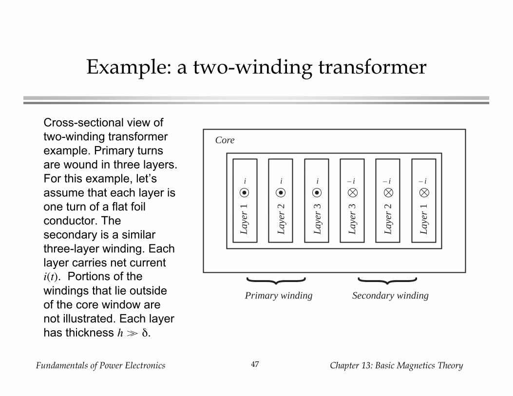
Cross-sectional view of
two-winding transformer
example. Primary turns
are wound in three layers.
For this example, let’s
assume that each layer is
one turn of a flat foil
conductor. The
secondary is a similar
three-layer winding. Each
layer carries net current
i(t). Portions of the
windings that lie outside
of the core window are
not illustrated. Each layer
has thickness h > .
Fundamentals of Power Electronics Chapter 13: Basic Magnetics Theory48
Distribution of currents on surfaces ofconductors: two-winding example
Core
Lay
er 1
Lay
er 2
Lay
er 3
Lay
er 1
Lay
er 2
Lay
er 3
– i – i – ii i i
i – i 3i–2i2i 2i –2i i –i–3i
Currentdensity
J
hΦ 2Φ 3Φ 2Φ Φ
Lay
er 1
Lay
er 2
Lay
er 3
Secondary windingPrimary winding
Lay
er 1
Lay
er 2
Lay
er 3
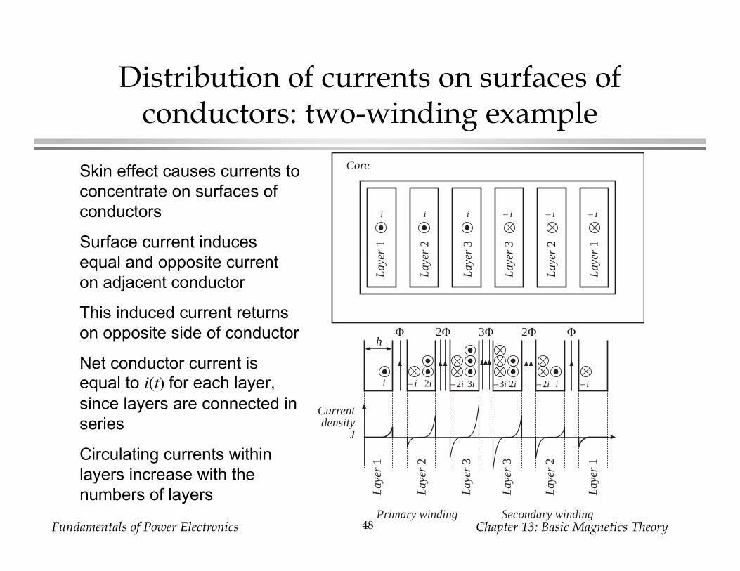
Skin effect causes currents to
concentrate on surfaces of
conductors
Surface current induces
equal and opposite current
on adjacent conductor
This induced current returns
on opposite side of conductor
Net conductor current isequal to i(t) for each layer,
since layers are connected in
series
Circulating currents within
layers increase with the
numbers of layers
Fundamentals of Power Electronics Chapter 13: Basic Magnetics Theory49
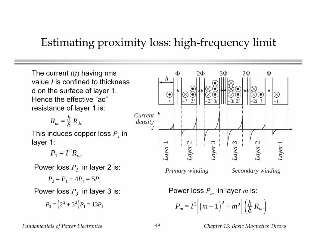
Estimating proximity loss: high-frequency limit
This induces copper loss P1 in
layer 1:
Power loss P2 in layer 2 is:
Power loss P3 in layer 3 is: Power loss Pm in layer m is:
i – i 3i–2i2i 2i –2i i –i–3i
Currentdensity
J
hΦ 2Φ 3Φ 2Φ Φ
Lay
er 1
Lay
er 2
Lay
er 3
Secondary windingPrimary winding
Lay
er 1
Lay
er 2
Lay
er 3
The current i(t) having rms
value I is confined to thickness
d on the surface of layer 1.
Hence the effective “ac”
resistance of layer 1 is:
Rac = hδ Rdc
P1 = I 2Rac
P2 = P1 + 4P1 = 5P1
P3 = 22 + 32 P1 = 13P1 Pm = I 2 m – 12
+ m2 hδ Rdc
Fundamentals of Power Electronics Chapter 13: Basic Magnetics Theory50
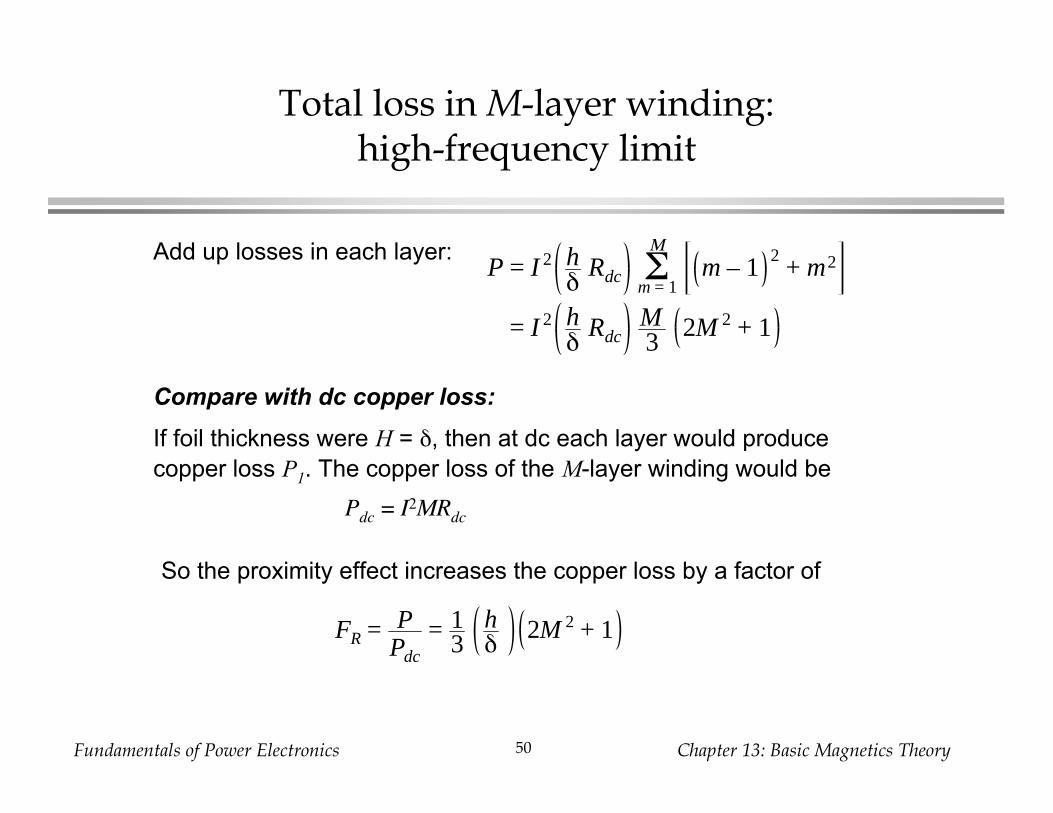
Total loss in M-layer winding:high-frequency limit
Add up losses in each layer:
Compare with dc copper loss:
If foil thickness were H = , then at dc each layer would produce
copper loss P1. The copper loss of the M-layer winding would be
So the proximity effect increases the copper loss by a factor of
P = I 2 hδ Rdc m – 1
2+ m2Σ
m = 1
Μ
= I 2 hδ Rdc
M3
2M 2 + 1
Pdc = I2MRdc
FR = PPdc
= 13
hδ 2M 2 + 1
Fundamentals of Power Electronics Chapter 13: Basic Magnetics Theory51
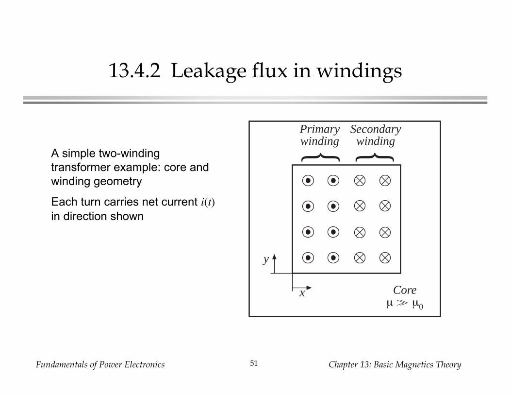
13.4.2 Leakage flux in windings
x
y
Primarywinding
Secondarywinding{
Coreµ > µ0
{A simple two-winding
transformer example: core and
winding geometry
Each turn carries net current i(t)
in direction shown
Fundamentals of Power Electronics Chapter 13: Basic Magnetics Theory52
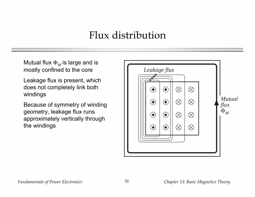
Flux distribution
Leakage flux
MutualfluxΦM
Mutual flux M is large and is
mostly confined to the core
Leakage flux is present, which
does not completely link both
windings
Because of symmetry of winding
geometry, leakage flux runs
approximately vertically through
the windings
Fundamentals of Power Electronics Chapter 13: Basic Magnetics Theory53
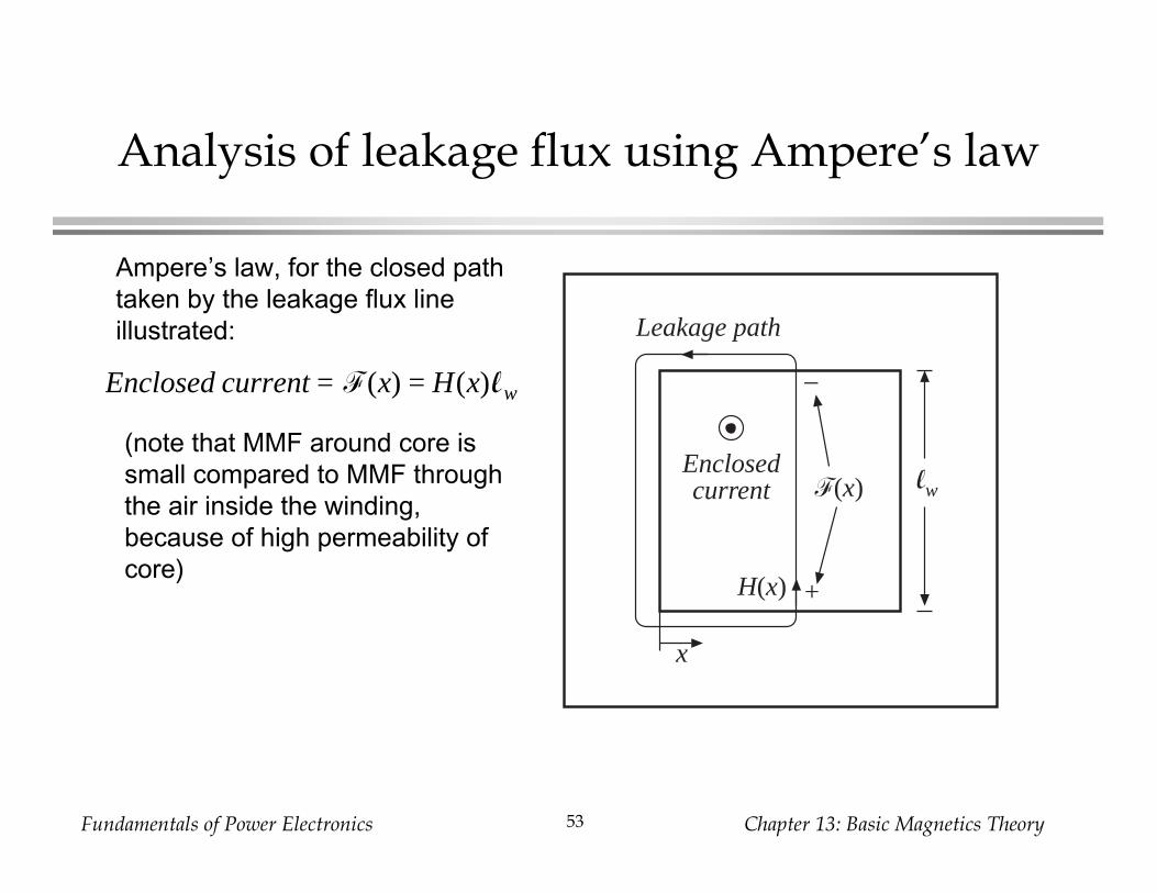
Analysis of leakage flux using Ampere’s law
x
lwF(x)
+
–
H(x)
Enclosedcurrent
Leakage path
Enclosed current = F(x) = H(x)lw
Ampere’s law, for the closed path
taken by the leakage flux line
illustrated:
(note that MMF around core is
small compared to MMF through
the air inside the winding,
because of high permeability of
core)
Fundamentals of Power Electronics Chapter 13: Basic Magnetics Theory54
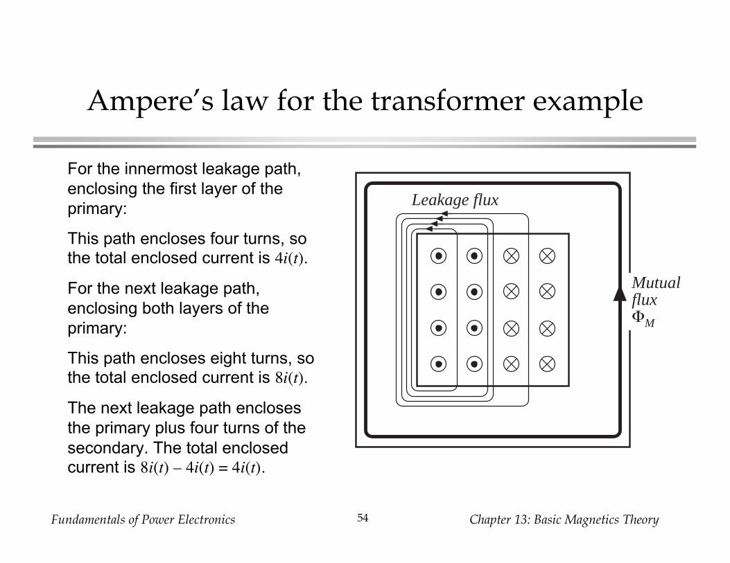
Ampere’s law for the transformer example
Leakage flux
MutualfluxΦM
For the innermost leakage path,
enclosing the first layer of the
primary:
This path encloses four turns, sothe total enclosed current is 4i(t).
For the next leakage path,
enclosing both layers of the
primary:
This path encloses eight turns, sothe total enclosed current is 8i(t).
The next leakage path encloses
the primary plus four turns of the
secondary. The total enclosedcurrent is 8i(t) – 4i(t) = 4i(t).
Fundamentals of Power Electronics Chapter 13: Basic Magnetics Theory55
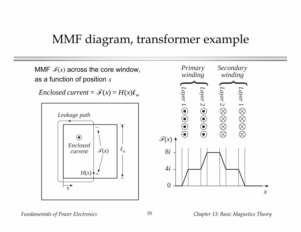
MMF diagram, transformer example
x
lwF(x)
+
–
H(x)
Enclosedcurrent
Leakage path
x
F(x)
Primarywinding
Secondarywinding{ {
0
8i
4i
Layer 1
Layer 2
Layer 2
Layer 1
MMF F(x) across the core window,
as a function of position x
Enclosed current = F(x) = H(x)lw
Fundamentals of Power Electronics Chapter 13: Basic Magnetics Theory56
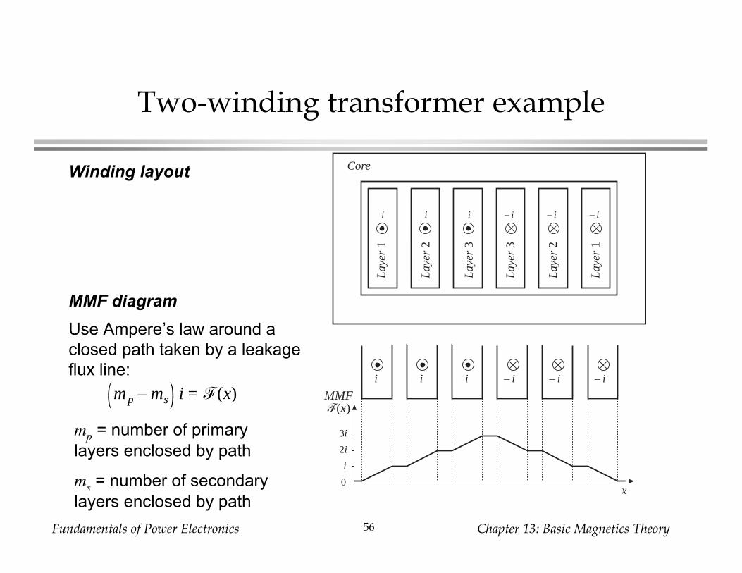
Two-winding transformer example
Core
Lay
er 1
Lay
er 2
Lay
er 3
Lay
er 1
Lay
er 2
Lay
er 3
– i – i – ii i i
x
F(x)
i i i – i – i – i
0
i
2i
3i
MMF
Winding layout
MMF diagram
mp – ms i = F(x)
Use Ampere’s law around a
closed path taken by a leakage
flux line:
mp = number of primary
layers enclosed by path
ms = number of secondary
layers enclosed by path
Fundamentals of Power Electronics Chapter 13: Basic Magnetics Theory57
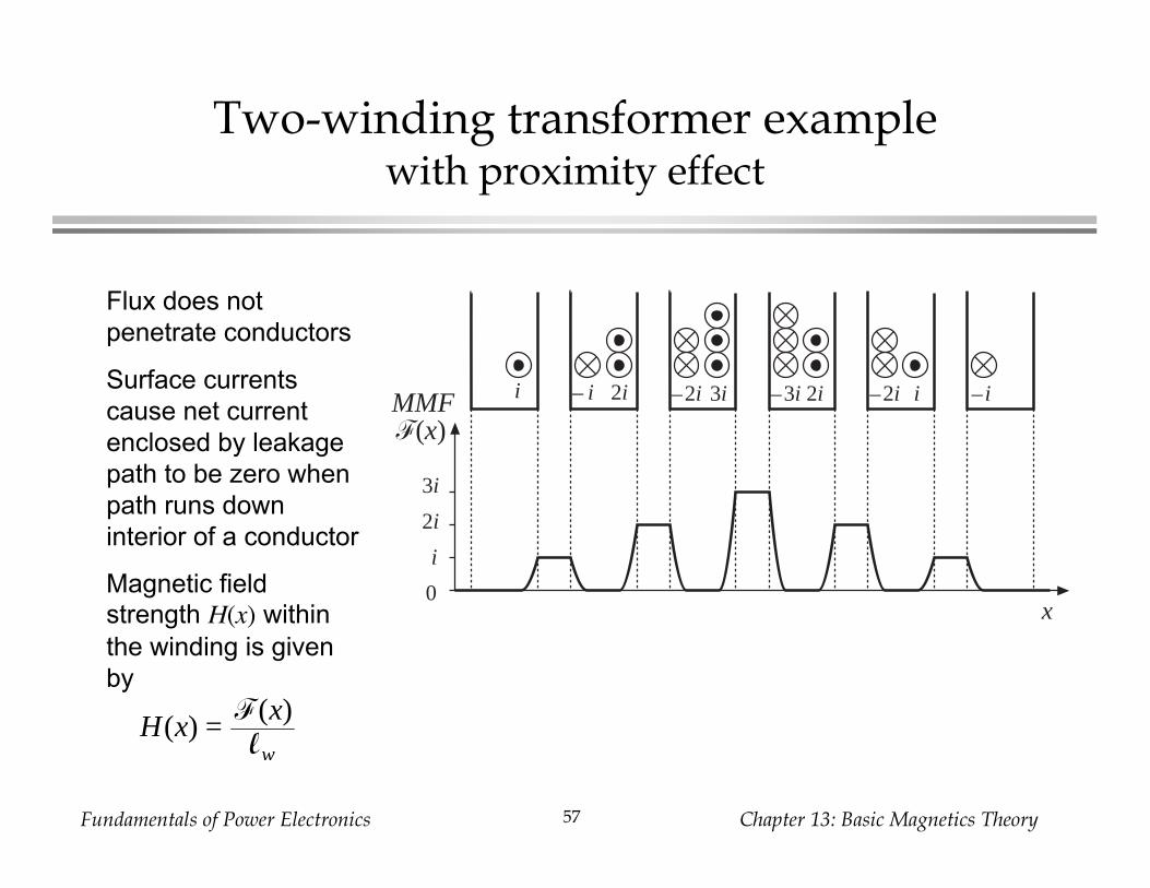
Two-winding transformer examplewith proximity effect
x
F(x)
0
i
2i
3i
MMF i – i 3i–2i2i 2i –2i i –i–3i
Flux does not
penetrate conductors
Surface currents
cause net current
enclosed by leakage
path to be zero when
path runs down
interior of a conductor
Magnetic field
strength H(x) within
the winding is given
by
H(x) =F(x)lw
Fundamentals of Power Electronics Chapter 13: Basic Magnetics Theory58
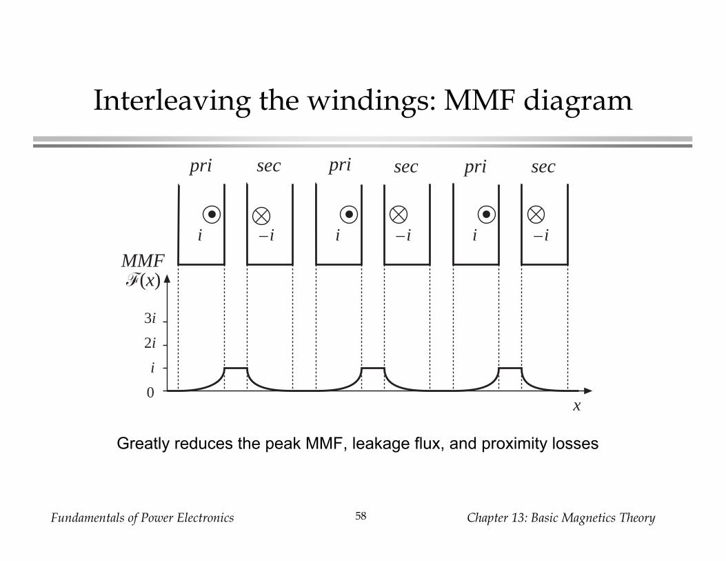
Interleaving the windings: MMF diagram
x
F(x)
i ii –i–i –i
0
i
2i
3i
MMF
pri sec pri sec pri sec
Greatly reduces the peak MMF, leakage flux, and proximity losses
Fundamentals of Power Electronics Chapter 13: Basic Magnetics Theory59
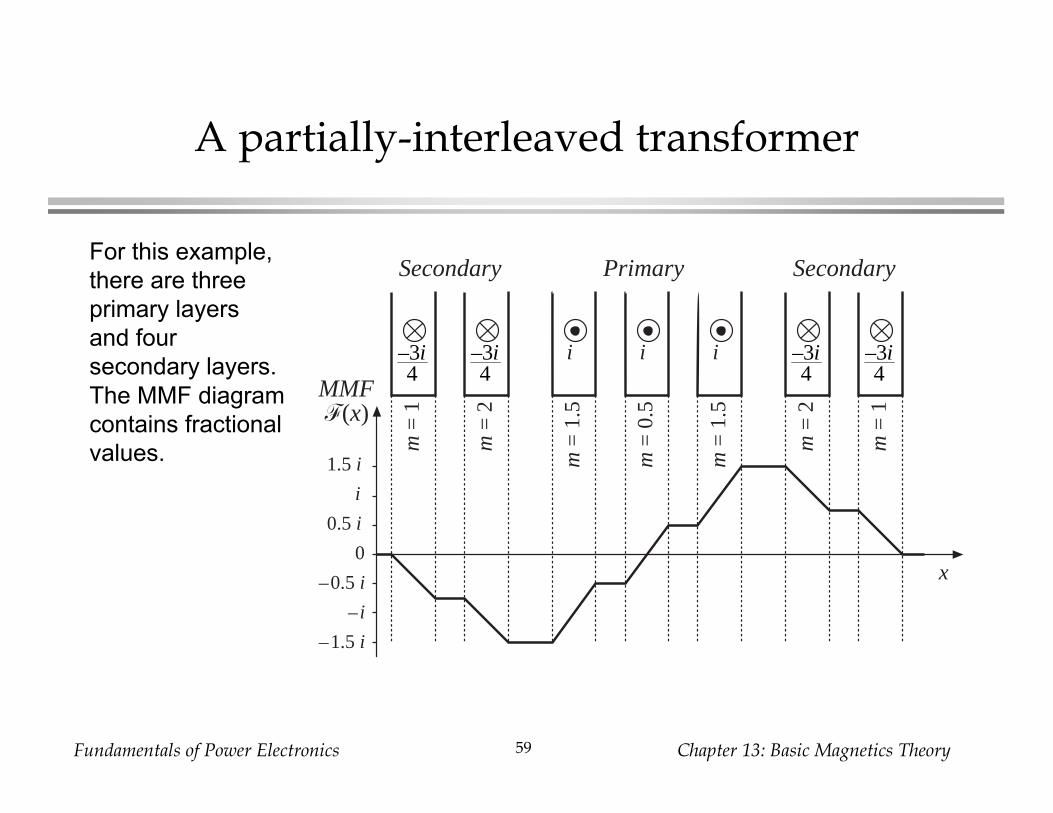
A partially-interleaved transformer
x
F(x)MMF
–3i4
–3i4
i i i –3i4
–3i4
PrimarySecondary Secondary
0
0.5 i
i
1.5 i
–0.5 i
– i
–1.5 i
m =
1
m =
1
m =
2
m =
2
m =
1.5
m =
1.5
m =
0.5
For this example,
there are three
primary layers
and four
secondary layers.
The MMF diagram
contains fractional
values.
Fundamentals of Power Electronics Chapter 13: Basic Magnetics Theory60
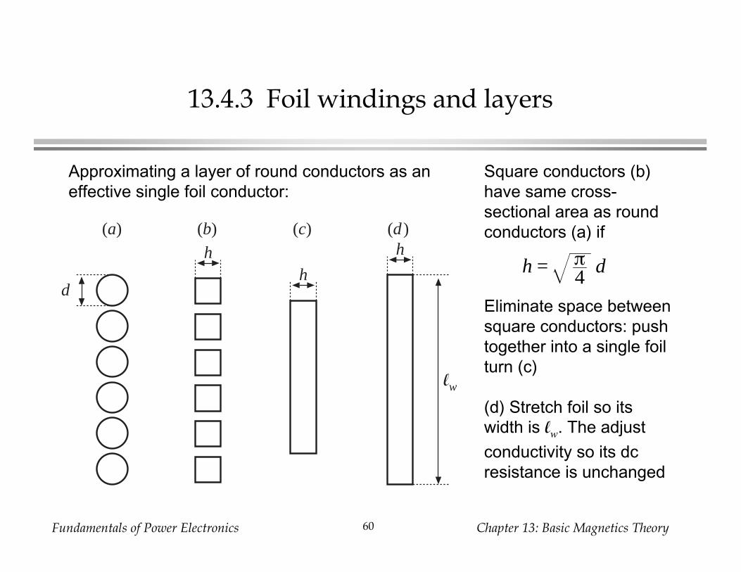
13.4.3 Foil windings and layers
Eliminate space between
square conductors: push
together into a single foil
turn (c)
(d) Stretch foil so its
width is lw. The adjust
conductivity so its dc
resistance is unchanged
(a) (b) (c) (d )
d
lw
h h
h
Approximating a layer of round conductors as an
effective single foil conductor:
Square conductors (b)
have same cross-
sectional area as round
conductors (a) if
h = π4
d
Fundamentals of Power Electronics Chapter 13: Basic Magnetics Theory61
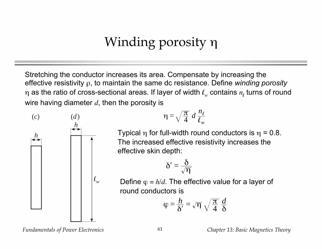
Winding porosity
(c) (d )
lw
h
h
Stretching the conductor increases its area. Compensate by increasing theeffective resistivity , to maintain the same dc resistance. Define winding porosity
as the ratio of cross-sectional areas. If layer of width lw contains nl turns of round
wire having diameter d, then the porosity is
η = π4
dnl
lw
Typical for full-width round conductors is = 0.8.
The increased effective resistivity increases the
effective skin depth:
δ′ = δη
Define = h/d. The effective value for a layer of
round conductors is
ϕ = hδ′
= η π4
dδ
Fundamentals of Power Electronics Chapter 13: Basic Magnetics Theory62
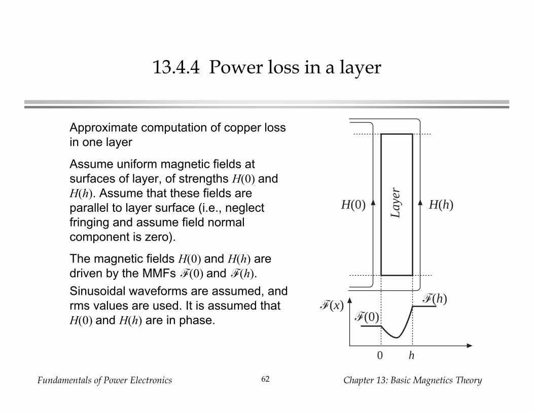
13.4.4 Power loss in a layer
Approximate computation of copper loss
in one layer
Assume uniform magnetic fields at
surfaces of layer, of strengths H(0) and
H(h). Assume that these fields are
parallel to layer surface (i.e., neglect
fringing and assume field normal
component is zero).
The magnetic fields H(0) and H(h) are
driven by the MMFs F(0) and F(h).
Sinusoidal waveforms are assumed, and
rms values are used. It is assumed that
H(0) and H(h) are in phase.
F(x)
0 h
F(h)
F(0)
H(0) H(h)
Lay
er
Fundamentals of Power Electronics Chapter 13: Basic Magnetics Theory63
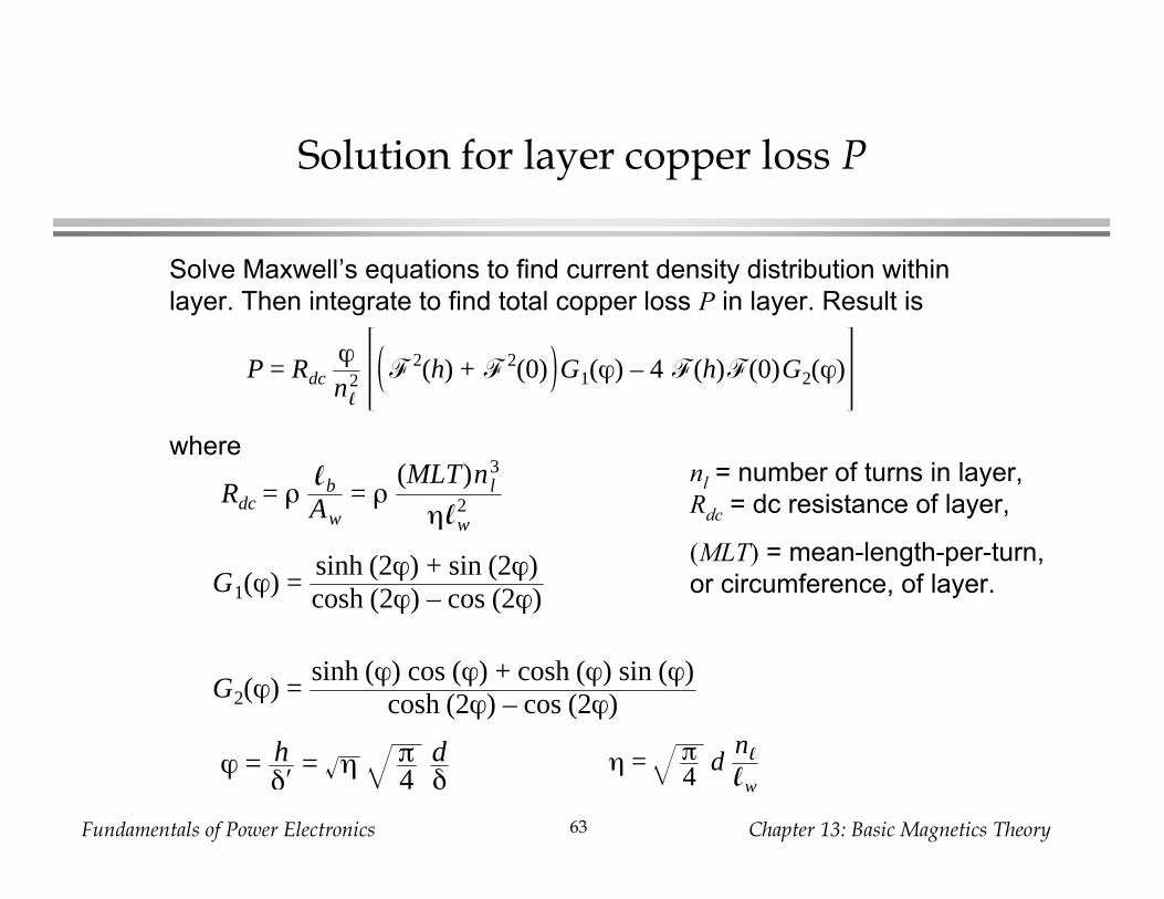
Solution for layer copper loss P
Solve Maxwell’s equations to find current density distribution within
layer. Then integrate to find total copper loss P in layer. Result is
wherenl = number of turns in layer,
Rdc = dc resistance of layer,
(MLT) = mean-length-per-turn,
or circumference, of layer.
P = Rdcϕnl
2 F
2(h) + F
2(0) G1(ϕ) – 4 F(h)F(0)G2(ϕ)
Rdc = ρlb
Aw= ρ
(MLT)nl3
ηlw2
G1(ϕ) =sinh (2ϕ) + sin (2ϕ)cosh (2ϕ) – cos (2ϕ)
G2(ϕ) =sinh (ϕ) cos (ϕ) + cosh (ϕ) sin (ϕ)
cosh (2ϕ) – cos (2ϕ)
η = π4
dnl
lwϕ = h
δ′= η π
4dδ
Fundamentals of Power Electronics Chapter 13: Basic Magnetics Theory64
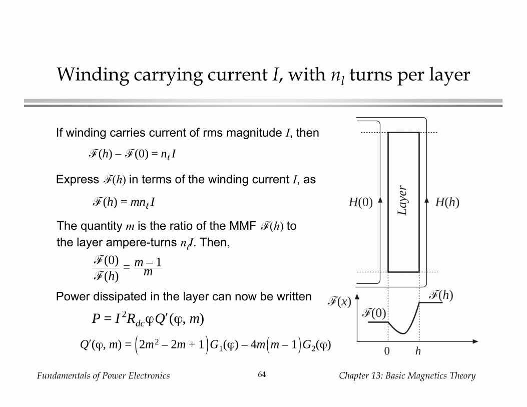
Winding carrying current I, with nl turns per layer
If winding carries current of rms magnitude I, then
Express F(h) in terms of the winding current I, as
The quantity m is the ratio of the MMF F(h) to
the layer ampere-turns nlI. Then,
Power dissipated in the layer can now be writtenF(x)
0 h
F(h)
F(0)
H(0) H(h)
Lay
er
F(h) – F(0) = nl
I
F(h) = mnl
I
F(0)F(h)
= m – 1m
P = I 2RdcϕQ′(ϕ, m)
Q′(ϕ, m) = 2m2 – 2m + 1 G1(ϕ) – 4m m – 1 G2(ϕ)
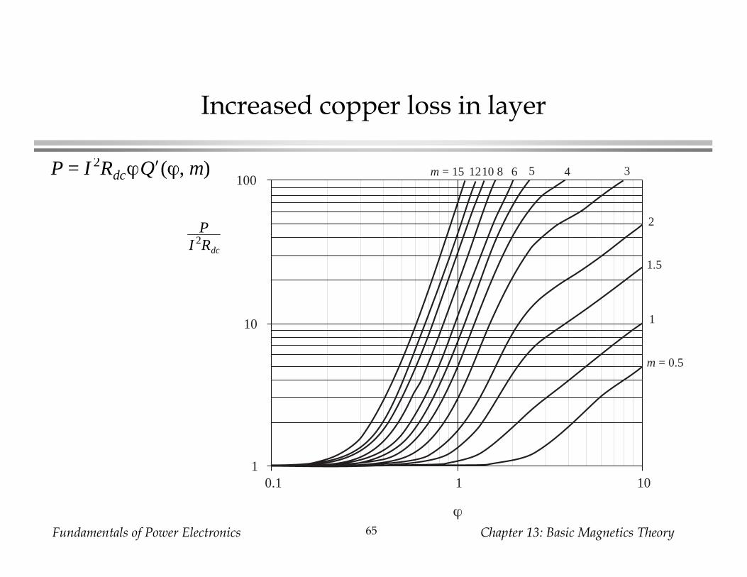
Fundamentals of Power Electronics Chapter 13: Basic Magnetics Theory65
Increased copper loss in layer
P = I 2RdcϕQ′(ϕ, m)
1
10
100
0.1 1 10
ϕ
PI 2Rdc
m = 0.5
1
1.5
2
345681012m = 15
Fundamentals of Power Electronics Chapter 13: Basic Magnetics Theory66
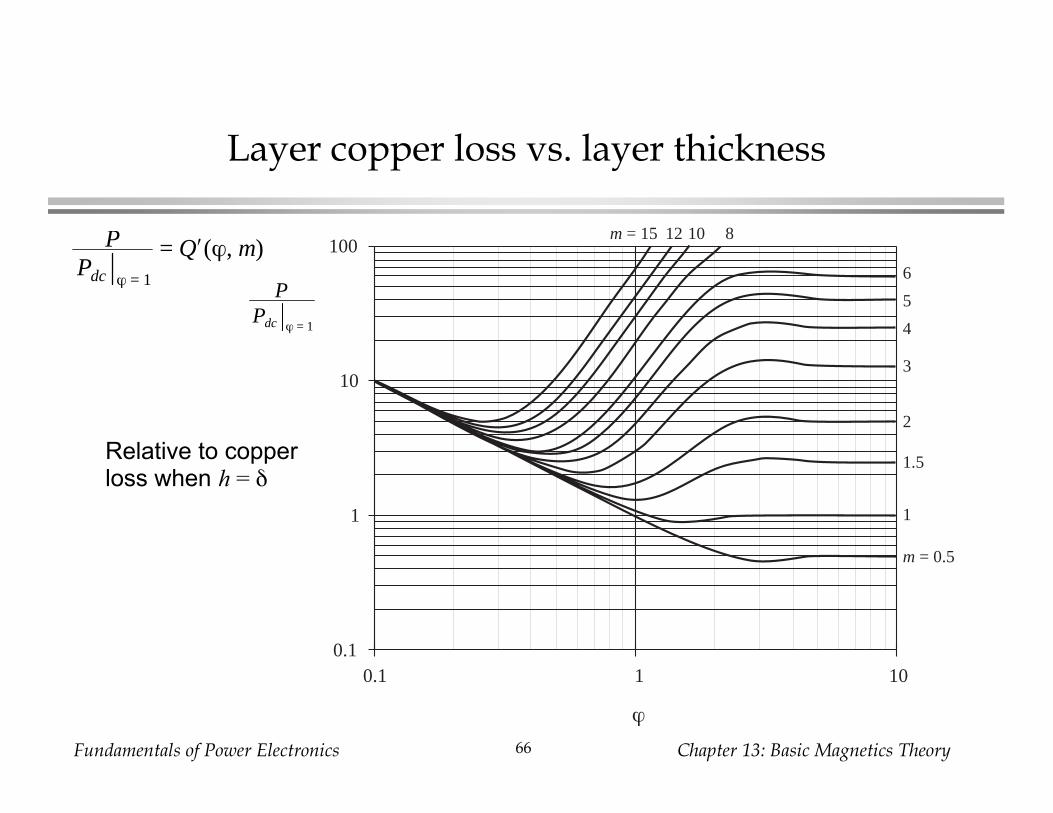
Layer copper loss vs. layer thickness
Relative to copperloss when h =
PPdc ϕ = 1
= Q′(ϕ, m)
0.1 1 100.1
1
10
100
ϕ
m = 0.5
1
1.5
2
3
4
5
6
81012m = 15
PPdc ϕ = 1
Fundamentals of Power Electronics Chapter 13: Basic Magnetics Theory67
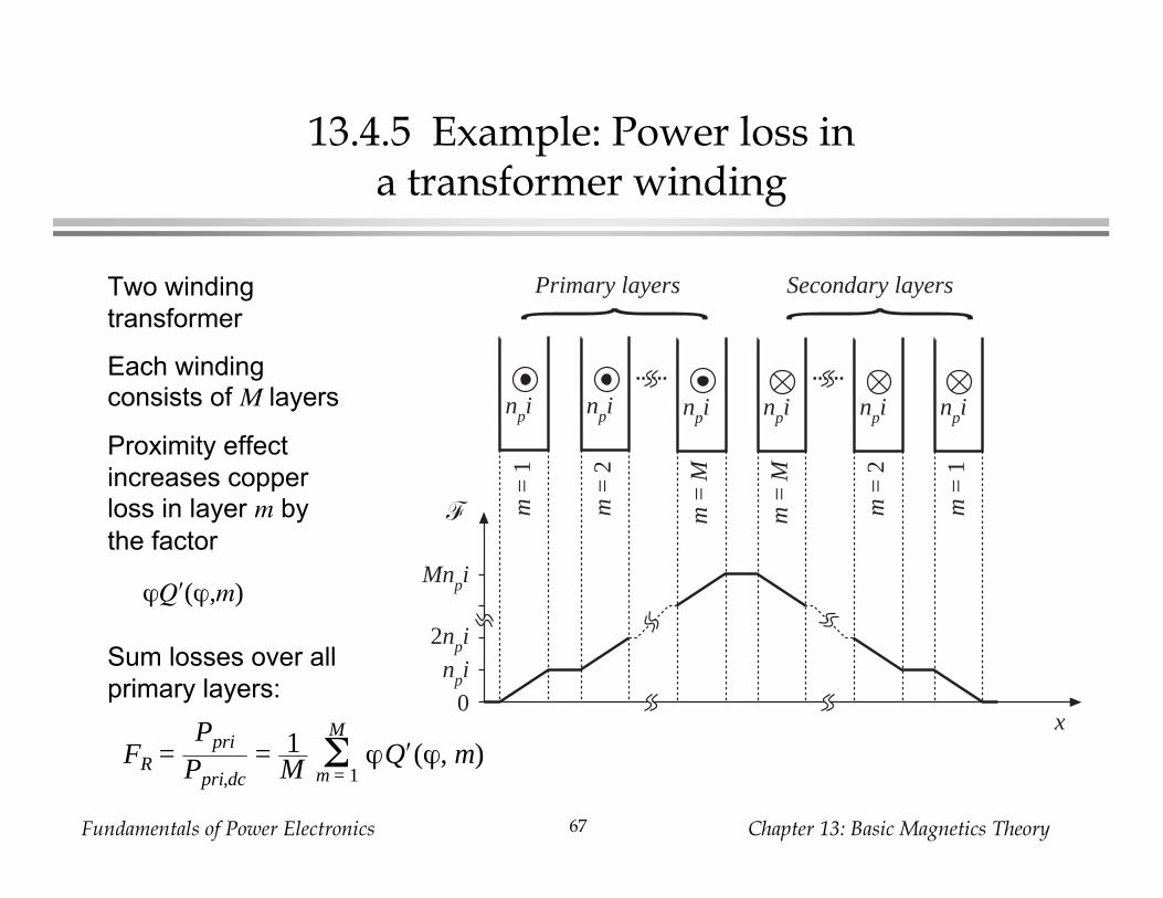
13.4.5 Example: Power loss ina transformer winding
Two winding
transformer
Each windingconsists of M layers
Proximity effect
increases copper
loss in layer m by
the factor
Sum losses over all
primary layers:
{x
npi npi npi npi npi npi
Primary layers Secondary layers{F
0npi
2npi
Mnpi
m =
1
m =
2
m =
M
m =
M
m =
2
m =
1
FR =Ppri
Ppri,dc= 1
M ϕQ′(ϕ, m)Σm = 1
M
Q ( ,m)
Fundamentals of Power Electronics Chapter 13: Basic Magnetics Theory68
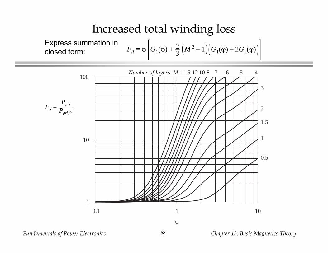
Increased total winding lossExpress summation in
closed form:
1
10
100
1010.1
0.5
1
1.5
2
3
ϕ
45678101215Number of layers M =
FR =Ppri
Ppri,dc
FR = ϕ G1(ϕ) + 23
M 2 – 1 G1(ϕ) – 2G2(ϕ)
Fundamentals of Power Electronics Chapter 13: Basic Magnetics Theory69
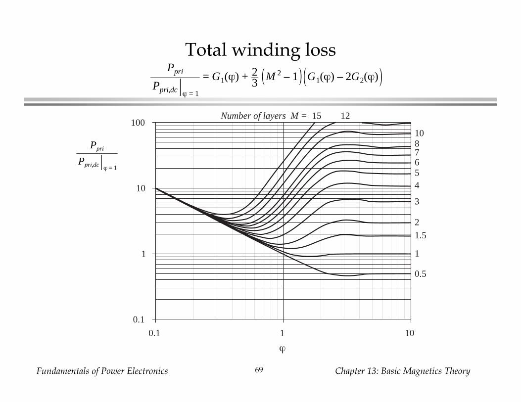
Total winding loss
0.1
1
10
100
0.1 1 10
0.5
1
1.52
3
4567810
1215Number of layers M =
ϕ
Ppri
Ppri,dc ϕ = 1
Ppri
Ppri,dc ϕ = 1
= G1(ϕ) + 23
M 2 – 1 G1(ϕ) – 2G2(ϕ)
Fundamentals of Power Electronics Chapter 13: Basic Magnetics Theory70
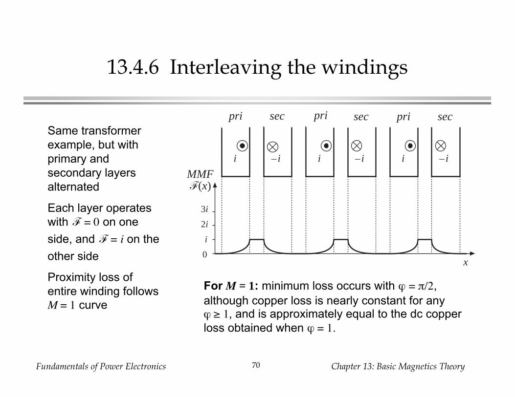
13.4.6 Interleaving the windings
x
F(x)
i ii –i–i –i
0
i
2i
3i
MMF
pri sec pri sec pri secSame transformer
example, but with
primary and
secondary layers
alternated
Each layer operates
with F = 0 on one
side, and F = i on the
other side
Proximity loss of
entire winding follows
M = 1 curve
For M = 1: minimum loss occurs with = /2,
although copper loss is nearly constant for any1, and is approximately equal to the dc copper
loss obtained when = 1.
Fundamentals of Power Electronics Chapter 13: Basic Magnetics Theory71
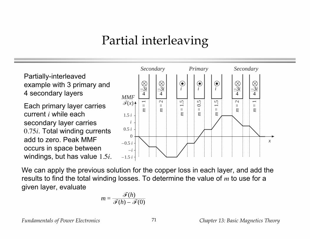
Partial interleaving
x
F(x)MMF
–3i4
–3i4
i i i –3i4
–3i4
PrimarySecondary Secondary
0
0.5 i
i
1.5 i
–0.5 i
– i
–1.5 i
m =
1
m =
1
m =
2
m =
2
m =
1.5
m =
1.5
m =
0.5
Partially-interleaved
example with 3 primary and
4 secondary layers
Each primary layer carriescurrent i while each
secondary layer carries0.75i. Total winding currents
add to zero. Peak MMF
occurs in space between
windings, but has value 1.5i.
We can apply the previous solution for the copper loss in each layer, and add the
results to find the total winding losses. To determine the value of m to use for a
given layer, evaluate
m =F(h)
F(h) – F(0)
Fundamentals of Power Electronics Chapter 13: Basic Magnetics Theory72
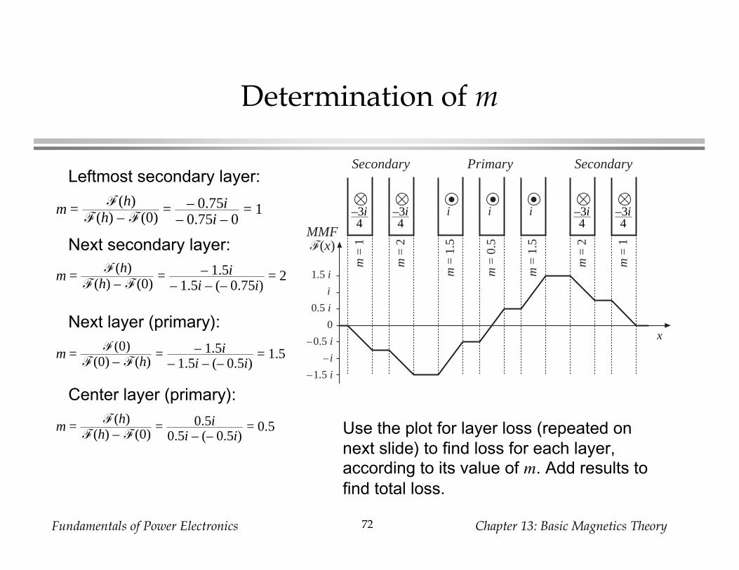
Determination of m
x
F(x)MMF
–3i4
–3i4
i i i –3i4
–3i4
PrimarySecondary Secondary
0
0.5 i
i
1.5 i
–0.5 i
– i
–1.5 i
m =
1
m =
1
m =
2
m =
2
m =
1.5
m =
1.5
m =
0.5
m =F(h)
F(h) – F(0)= – 0.75i
– 0.75i – 0= 1
Leftmost secondary layer:
m =F(h)
F(h) – F(0)= – 1.5i
– 1.5i – (– 0.75i)= 2
Next secondary layer:
Next layer (primary):
m =F(0)
F(0) – F(h)= – 1.5i
– 1.5i – (– 0.5i)= 1.5
Center layer (primary):
m =F(h)
F(h) – F(0)= 0.5i
0.5i – (– 0.5i)= 0.5 Use the plot for layer loss (repeated on
next slide) to find loss for each layer,
according to its value of m. Add results to
find total loss.

Fundamentals of Power Electronics Chapter 13: Basic Magnetics Theory73
Layer copper loss vs. layer thickness
Relative to copperloss when h =
PPdc ϕ = 1
= Q′(ϕ, m)
0.1 1 100.1
1
10
100
ϕ
m = 0.5
1
1.5
2
3
4
5
6
81012m = 15
PPdc ϕ = 1
Fundamentals of Power Electronics Chapter 13: Basic Magnetics Theory74
Discussion: design of winding geometryto minimize proximity loss
• Interleaving windings can significantly reduce the proximity loss when
the winding currents are in phase, such as in the transformers of buck-
derived converters or other converters
• In some converters (such as flyback or SEPIC) the winding currents are
out of phase. Interleaving then does little to reduce the peak MMF and
proximity loss. See Vandelac and Ziogas [10].
• For sinusoidal winding currents, there is an optimal conductor thicknessnear = 1 that minimizes copper loss.
• Minimize the number of layers. Use a core geometry that maximizes
the width lw of windings.
• Minimize the amount of copper in vicinity of high MMF portions of the
windings
Fundamentals of Power Electronics Chapter 13: Basic Magnetics Theory75
Litz wire
• A way to increase conductor area while maintaining lowproximity losses
• Many strands of small-gauge wire are bundled together and areexternally connected in parallel
• Strands are twisted, or transposed, so that each strand passesequally through each position on inside and outside of bundle.This prevents circulation of currents between strands.
• Strand diameter should be sufficiently smaller than skin depth
• The Litz wire bundle itself is composed of multiple layers
• Advantage: when properly sized, can significantly reduceproximity loss
• Disadvantage: increased cost and decreased amount of copperwithin core window
Fundamentals of Power Electronics Chapter 13: Basic Magnetics Theory76
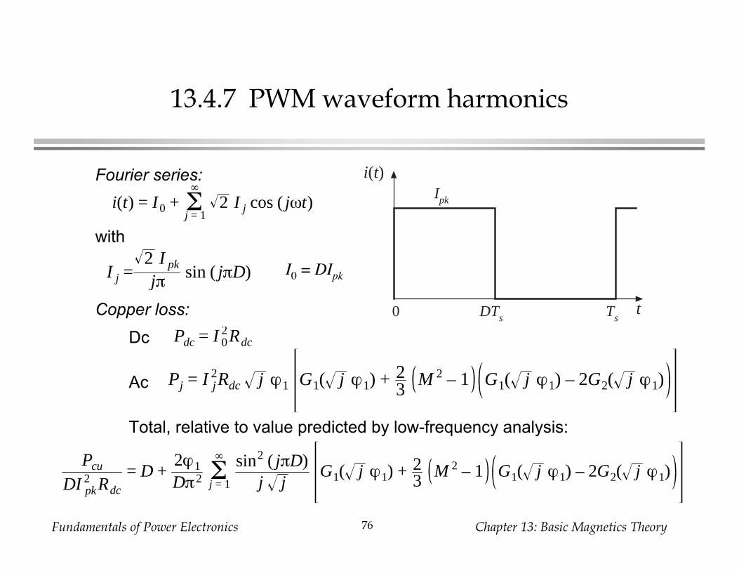
13.4.7 PWM waveform harmonics
Fourier series:
with
Copper loss:
Dc
Ac
Total, relative to value predicted by low-frequency analysis:
t
i(t)Ipk
DTs Ts0
i(t) = I0 + 2 I j cos ( jωt)Σj = 1
∞
I j =2 I pk
jπ sin ( jπD) I0 = DIpk
Pdc = I 02Rdc
Pj = I j2Rdc j ϕ1 G1( j ϕ1) + 2
3M 2 – 1 G1( j ϕ1) – 2G2( j ϕ1)
Pcu
DI pk2 Rdc
= D +2ϕ1
Dπ2sin2 ( jπD)
j jG1( j ϕ1) + 2
3M 2 – 1 G1( j ϕ1) – 2G2( j ϕ1)Σ
j = 1
∞
Fundamentals of Power Electronics Chapter 13: Basic Magnetics Theory77
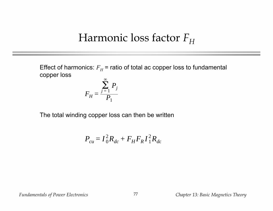
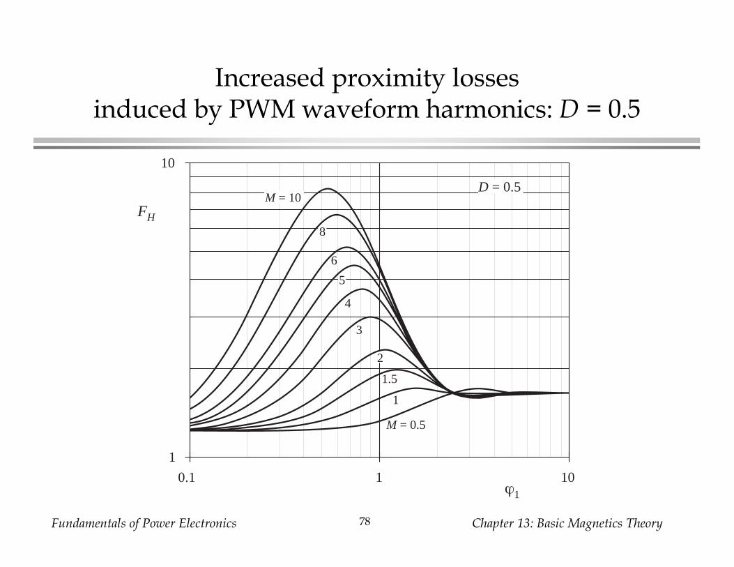
Harmonic loss factor FH
Effect of harmonics: FH = ratio of total ac copper loss to fundamental
copper loss
The total winding copper loss can then be written
FH =PjΣ
j = 1
∞
P1
Pcu = I 02Rdc + FH FR I 1
2Rdc
Fundamentals of Power Electronics Chapter 13: Basic Magnetics Theory78
Increased proximity lossesinduced by PWM waveform harmonics: D = 0.5
1
10
0.1 1 10ϕ1
FH
D = 0.5
M = 0.5
1
1.5
2
3
4
5
6
8
M = 10
Fundamentals of Power Electronics Chapter 13: Basic Magnetics Theory79
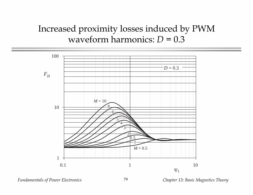
Increased proximity losses induced by PWMwaveform harmonics: D = 0.3
1
10
100
0.1 1 10ϕ1
FH
M = 0.5
11.5
2
34
5
68
M = 10
D = 0.3
Fundamentals of Power Electronics Chapter 13: Basic Magnetics Theory80
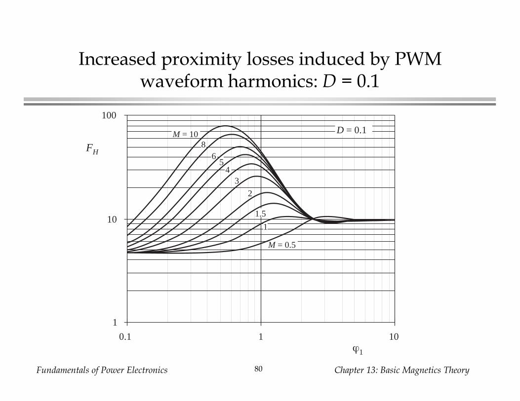
Increased proximity losses induced by PWMwaveform harmonics: D = 0.1
1
10
100
0.1 1 10ϕ1
FH
M = 0.5
1
1.5
2
34
56
8M = 10 D = 0.1
Fundamentals of Power Electronics Chapter 13: Basic Magnetics Theory81
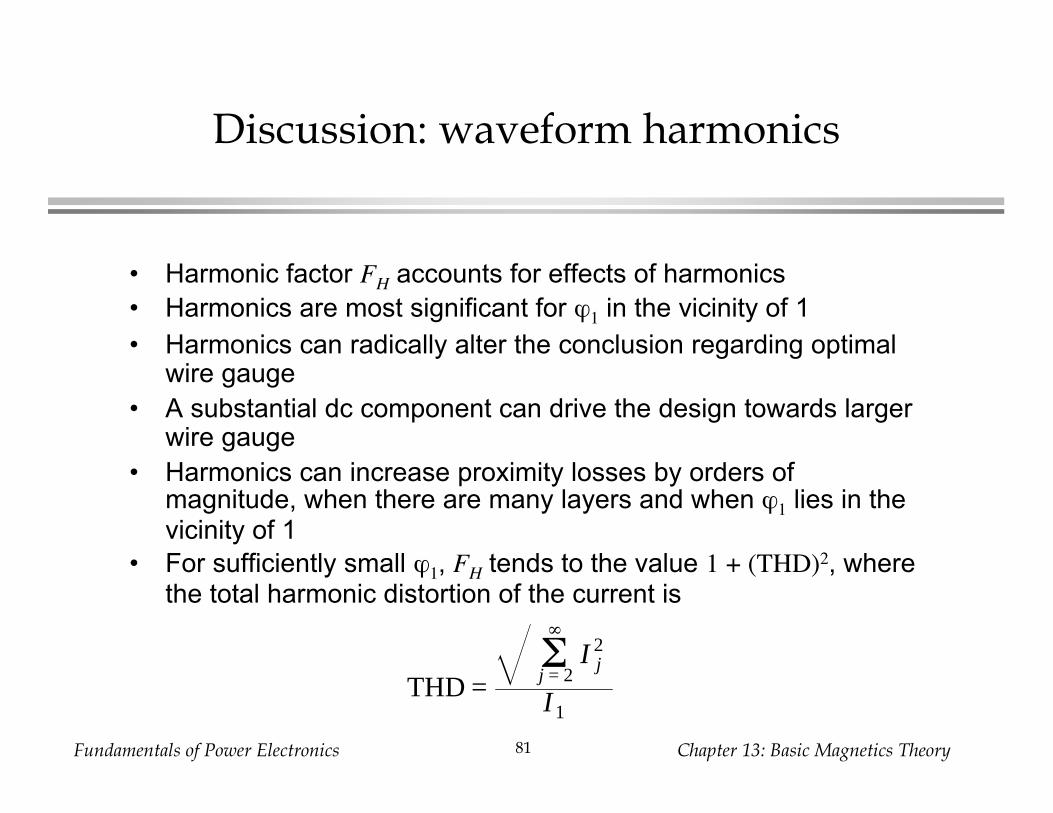
Discussion: waveform harmonics
• Harmonic factor FH accounts for effects of harmonics
• Harmonics are most significant for 1 in the vicinity of 1
• Harmonics can radically alter the conclusion regarding optimalwire gauge
• A substantial dc component can drive the design towards largerwire gauge
• Harmonics can increase proximity losses by orders ofmagnitude, when there are many layers and when 1 lies in thevicinity of 1
• For sufficiently small 1, FH tends to the value 1 + (THD)2, wherethe total harmonic distortion of the current is
THD =I j
2Σj = 2
∞
I1