BIRTH DEATH PROCESSES AND QUEUEING SYSTEMSpeople.unipmn.it/bobbio/DIDATTICA/MODQ/quecomp.pdf ·...
25
1 BIRTH DEATH PROCESSES AND QUEUEING SYSTEMS Andrea Bobbio Anno Accademico 1999-2000
Transcript of BIRTH DEATH PROCESSES AND QUEUEING SYSTEMSpeople.unipmn.it/bobbio/DIDATTICA/MODQ/quecomp.pdf ·...
1
BIRTH DEATH PROCESSES
AND
QUEUEING SYSTEMS
Andrea Bobbio
Anno Accademico 1999-2000
Queueing Systems 2
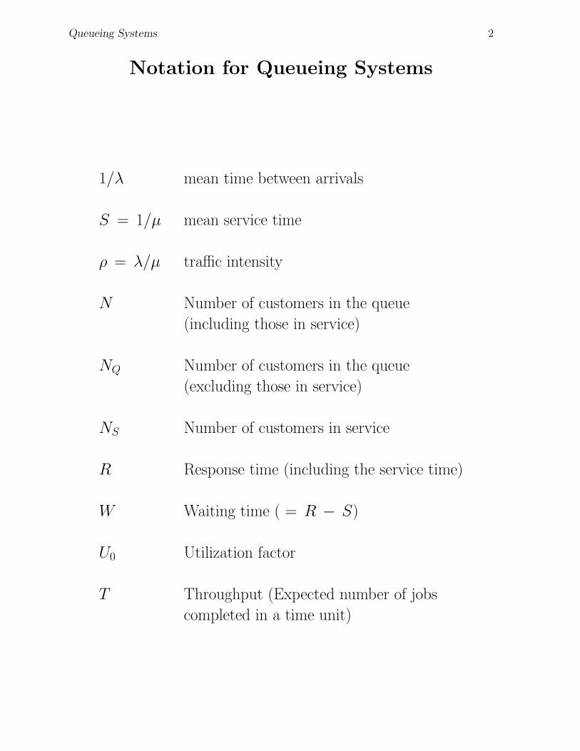
Notation for Queueing Systems
1/λ mean time between arrivals
S = 1/µ mean service time
ρ = λ/µ traffic intensity
N Number of customers in the queue
(including those in service)
NQ Number of customers in the queue
(excluding those in service)
NS Number of customers in service
R Response time (including the service time)
W Waiting time ( = R − S)
U0 Utilization factor
T Throughput (Expected number of jobs
completed in a time unit)
Queueing Systems 3
Birth-Death Processes
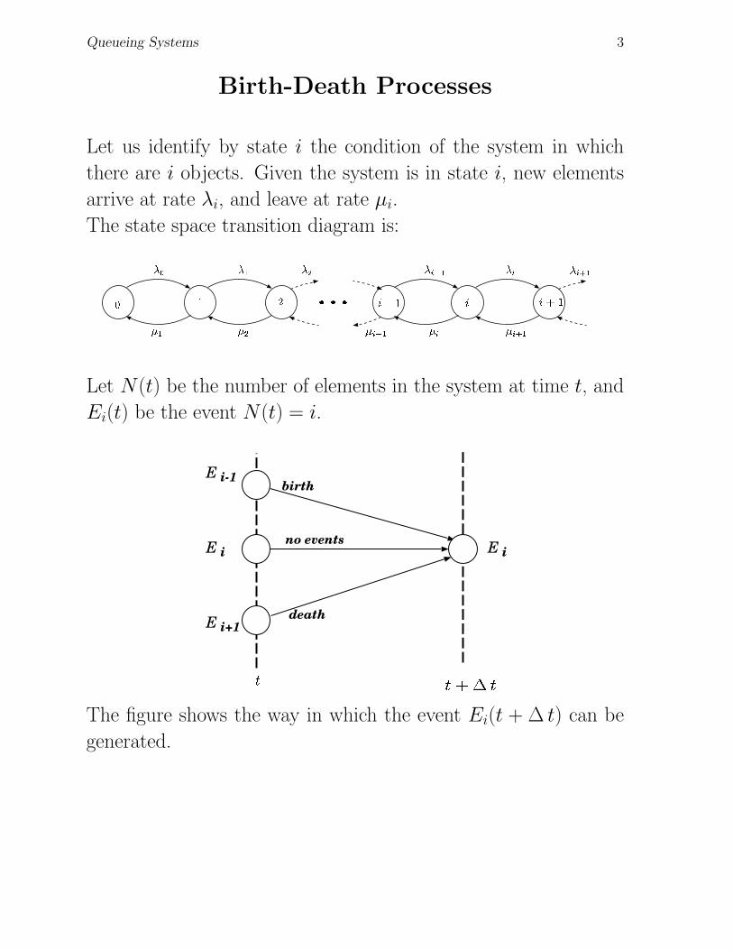
Let us identify by state i the condition of the system in which
there are i objects. Given the system is in state i, new elements
arrive at rate λi, and leave at rate µi.
The state space transition diagram is:
���
���
����� �
��� ��� �������
��� ������ !�"
#$#$# %�&('
)+* ,�-/.�0
1�2/3�4
Let N(t) be the number of elements in the system at time t, and
Ei(t) be the event N(t) = i.
E
E
E
Ei
i-1
i+1
i
birth
no events
death
� �������
The figure shows the way in which the event Ei(t + ∆ t) can be
generated.
Queueing Systems 4
Birth-Death Processes
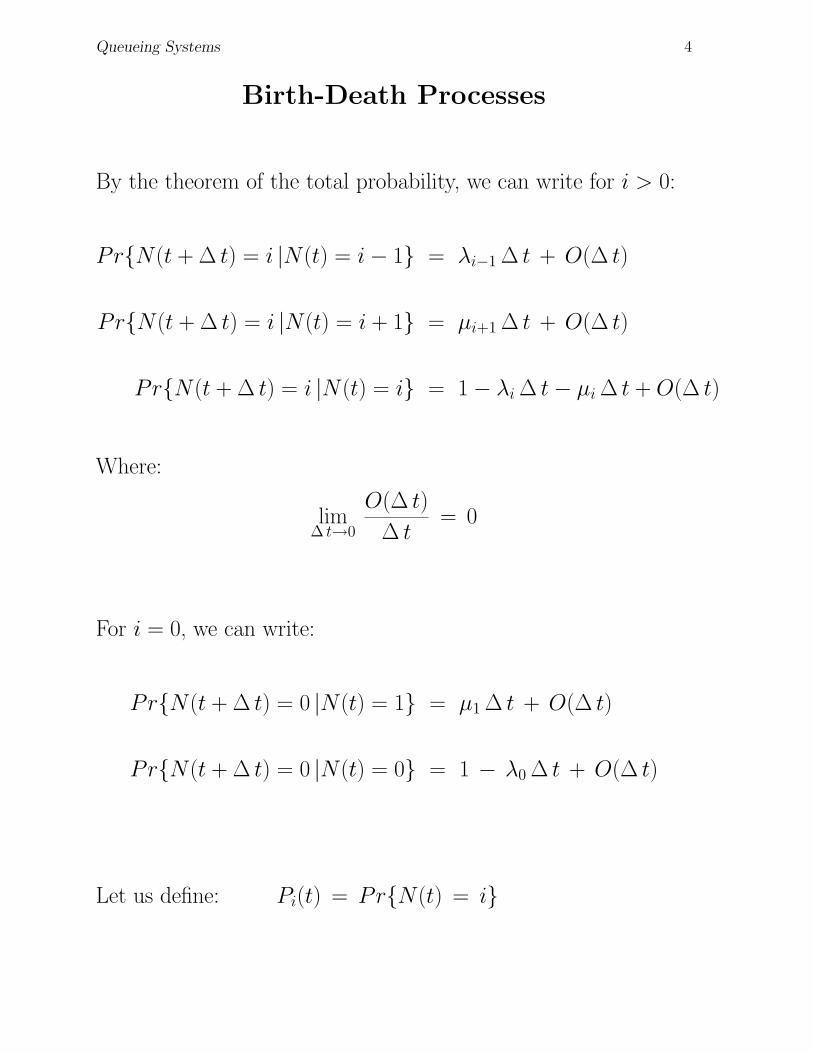
By the theorem of the total probability, we can write for i > 0:
Pr{N(t + ∆ t) = i |N(t) = i− 1} = λi−1 ∆ t + O(∆ t)
Pr{N(t + ∆ t) = i |N(t) = i + 1} = µi+1 ∆ t + O(∆ t)
Pr{N(t + ∆ t) = i |N(t) = i} = 1− λi ∆ t− µi ∆ t + O(∆ t)
Where:
lim∆ t→0
O(∆ t)
∆ t= 0
For i = 0, we can write:
Pr{N(t + ∆ t) = 0 |N(t) = 1} = µ1 ∆ t + O(∆ t)
Pr{N(t + ∆ t) = 0 |N(t) = 0} = 1 − λ0 ∆ t + O(∆ t)
Let us define: Pi(t) = Pr{N(t) = i}
Queueing Systems 5
Birth-Death Processes
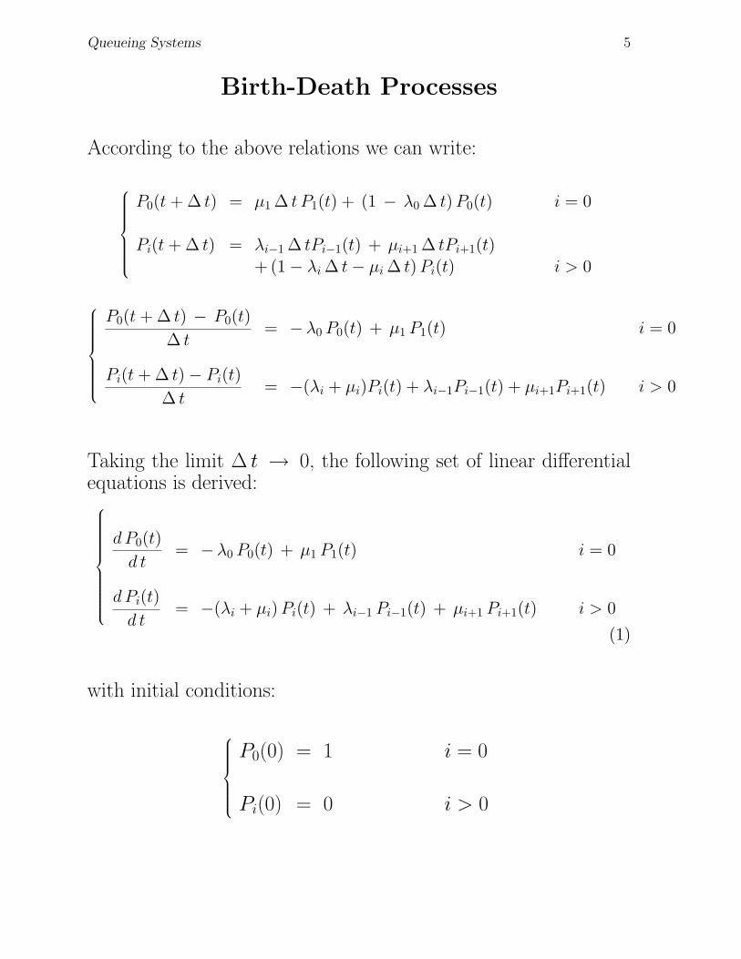
According to the above relations we can write:
P0(t + ∆ t) = µ1 ∆ t P1(t) + (1 − λ0 ∆ t) P0(t) i = 0
Pi(t + ∆ t) = λi−1 ∆ tPi−1(t) + µi+1 ∆ tPi+1(t)+ (1− λi ∆ t− µi ∆ t) Pi(t) i > 0
P0(t + ∆ t) − P0(t)
∆ t= −λ0 P0(t) + µ1 P1(t) i = 0
Pi(t + ∆ t)− Pi(t)
∆ t= −(λi + µi)Pi(t) + λi−1Pi−1(t) + µi+1Pi+1(t) i > 0
Taking the limit ∆ t → 0, the following set of linear differentialequations is derived:
dP0(t)
d t= −λ0 P0(t) + µ1 P1(t) i = 0
dPi(t)
d t= −(λi + µi) Pi(t) + λi−1 Pi−1(t) + µi+1 Pi+1(t) i > 0
(1)
with initial conditions:
P0(0) = 1 i = 0
Pi(0) = 0 i > 0
Queueing Systems 6
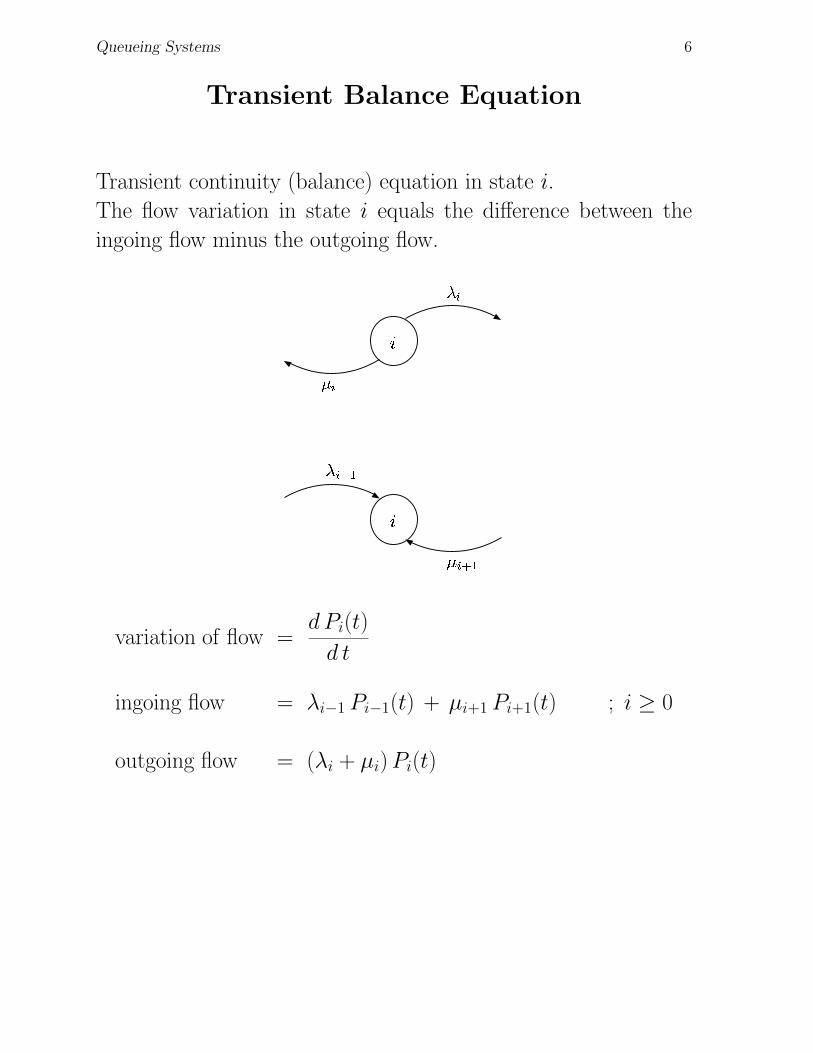
Transient Balance Equation
Transient continuity (balance) equation in state i.
The flow variation in state i equals the difference between the
ingoing flow minus the outgoing flow.
�
���
���
�
��� �
�������
variation of flow =dPi(t)
d t
ingoing flow = λi−1 Pi−1(t) + µi+1 Pi+1(t) ; i ≥ 0
outgoing flow = (λi + µi) Pi(t)
Queueing Systems 7
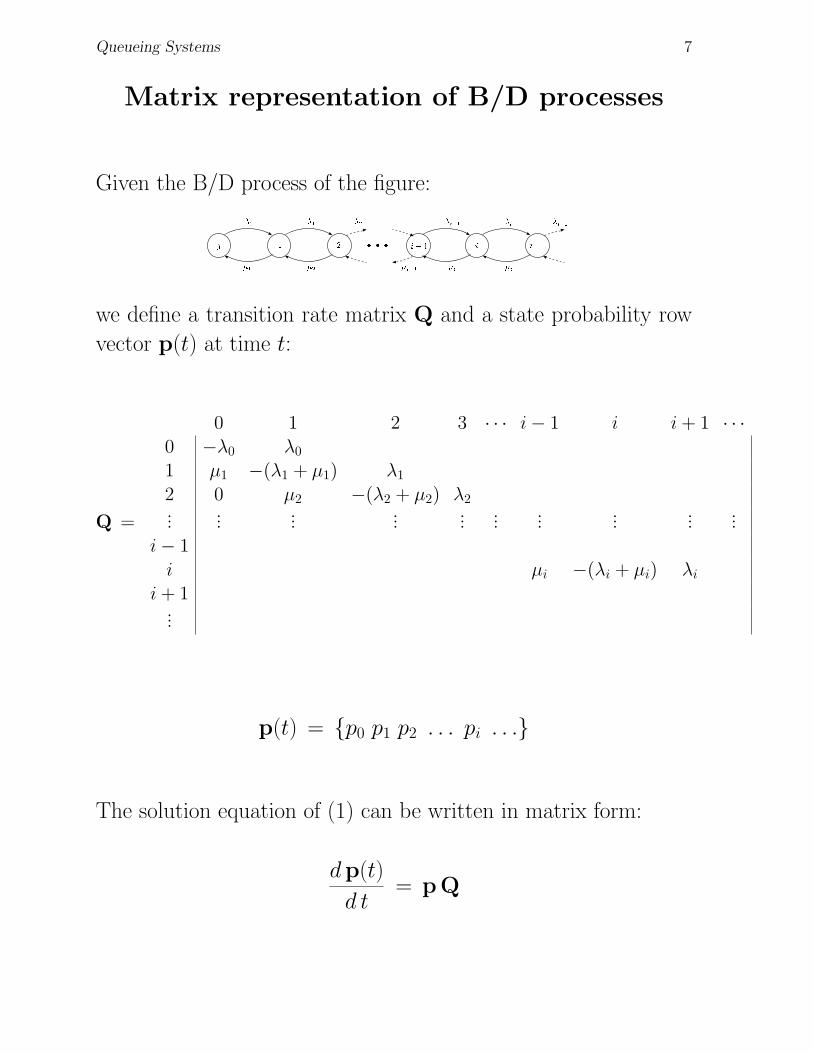
Matrix representation of B/D processes
Given the B/D process of the figure:���
���
����� �
��� ��� �������
��� ������ !�"
#$#$# %�&('
)+* ,�-/.�0
1�2/3�4
we define a transition rate matrix Q and a state probability row
vector p(t) at time t:
Q =
0 1 2 3 · · · i− 1 i i + 1 · · ·0 −λ0 λ0
1 µ1 −(λ1 + µ1) λ1
2 0 µ2 −(λ2 + µ2) λ2...
......
......
......
......
...i− 1
i µi −(λi + µi) λi
i + 1...
p(t) = {p0 p1 p2 . . . pi . . .}
The solution equation of (1) can be written in matrix form:
dp(t)
d t= pQ
Queueing Systems 8
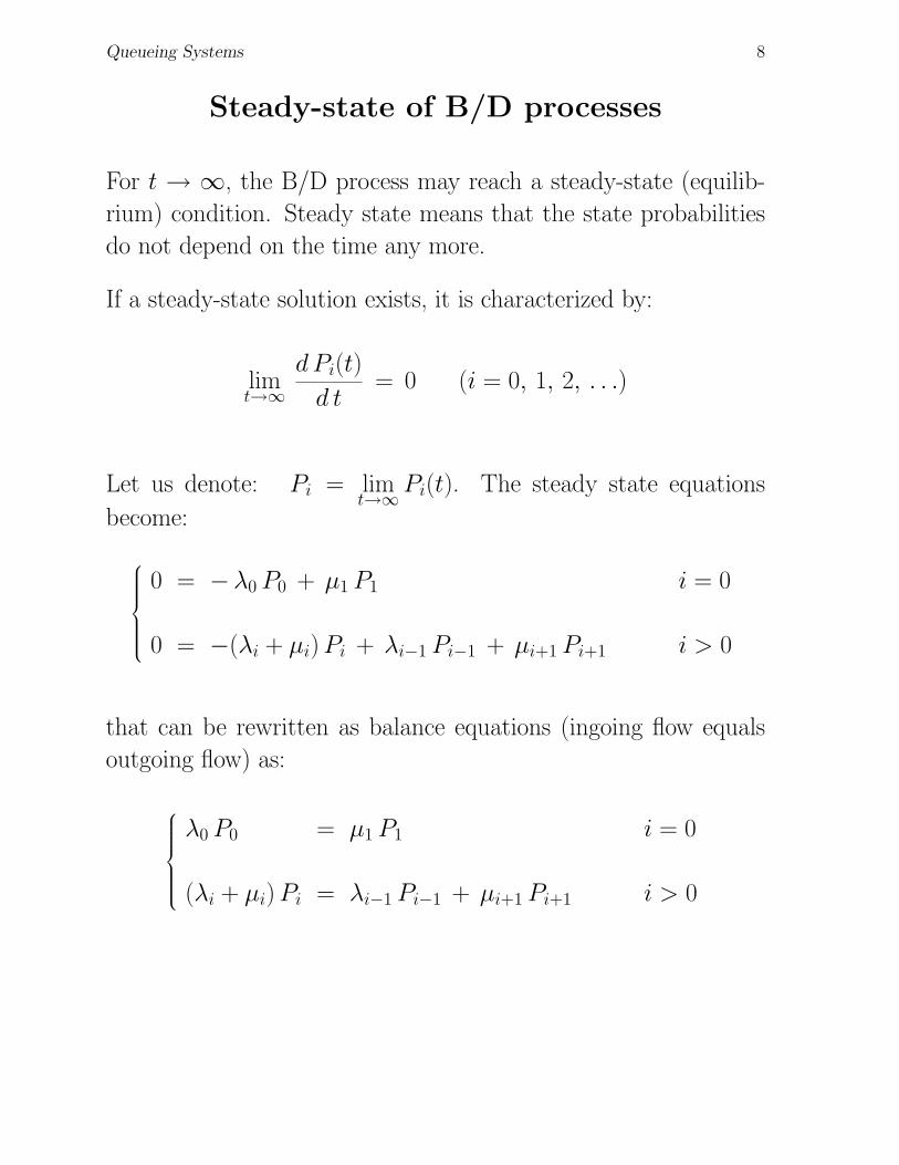
Steady-state of B/D processes
For t → ∞, the B/D process may reach a steady-state (equilib-
rium) condition. Steady state means that the state probabilities
do not depend on the time any more.
If a steady-state solution exists, it is characterized by:
limt→∞
dPi(t)
d t= 0 (i = 0, 1, 2, . . .)
Let us denote: Pi = limt→∞Pi(t). The steady state equations
become:
0 = −λ0 P0 + µ1 P1 i = 0
0 = −(λi + µi) Pi + λi−1 Pi−1 + µi+1 Pi+1 i > 0
that can be rewritten as balance equations (ingoing flow equals
outgoing flow) as:
λ0 P0 = µ1 P1 i = 0
(λi + µi) Pi = λi−1 Pi−1 + µi+1 Pi+1 i > 0
Queueing Systems 9
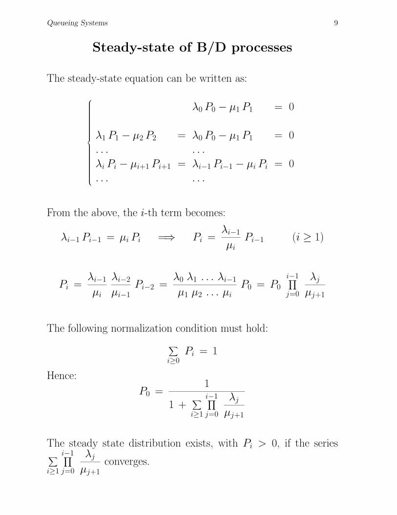
Steady-state of B/D processes
The steady-state equation can be written as:
λ0 P0 − µ1 P1 = 0
λ1 P1 − µ2 P2 = λ0 P0 − µ1 P1 = 0
. . . . . .
λi Pi − µi+1 Pi+1 = λi−1 Pi−1 − µi Pi = 0
. . . . . .
From the above, the i-th term becomes:
λi−1 Pi−1 = µi Pi =⇒ Pi =λi−1
µiPi−1 (i ≥ 1)
Pi =λi−1
µi
λi−2
µi−1Pi−2 =
λ0 λ1 . . . λi−1
µ1 µ2 . . . µiP0 = P0
i−1∏
j=0
λj
µj+1
The following normalization condition must hold:
∑
i≥0Pi = 1
Hence:
P0 =1
1 +∑
i≥1
i−1∏
j=0
λj
µj+1
The steady state distribution exists, with Pi > 0, if the series∑
i≥1
i−1∏
j=0
λj
µj+1converges.
Queueing Systems 10
Standard notation for queueing systems
The standard notation to identify the main elements that de-
fine the structure of a queueing system is the following (due to
Kendall):
A/B/c/d/e
where:
A Is the distribution of the interarrival times;
B Is the distribution of the service times;
c Is the number of servers;
d Is the storage capacity of the system (number of servers plus
the storage capacity of the buffer);
e Is the number of sources that provide clients.
The usual assumption for the interarrival and service time distri-
butions A and B is:
M Markovian (or exponential);
G General.
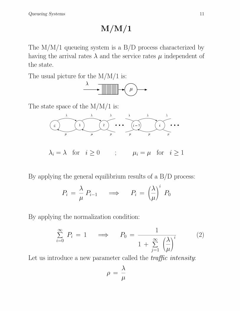
Queueing Systems 11
M/M/1
The M/M/1 queueing system is a B/D process characterized by
having the arrival rates λ and the service rates µ independent of
the state.
The usual picture for the M/M/1 is:�
�
The state space of the M/M/1 is:�
�
�������
� � � �
� � � � �
����� �����
λi = λ for i ≥ 0 ; µi = µ for i ≥ 1
By applying the general equilibrium results of a B/D process:
Pi =λ
µPi−1 =⇒ Pi =
λ
µ
i
P0
By applying the normalization condition:
∞∑i=0
Pi = 1 =⇒ P0 =1
1 +∞∑
j=1
λ
µ
i (2)
Let us introduce a new parameter called the traffic intensity:
ρ =λ
µ
Queueing Systems 12
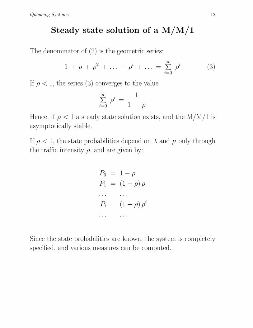
Steady state solution of a M/M/1
The denominator of (2) is the geometric series:
1 + ρ + ρ2 + . . . + ρi + . . . =∞∑i=0
ρi (3)
If ρ < 1, the series (3) converges to the value
∞∑i=0
ρi =1
1 − ρ
Hence, if ρ < 1 a steady state solution exists, and the M/M/1 is
asymptotically stable.
If ρ < 1, the state probabilities depend on λ and µ only through
the traffic intensity ρ, and are given by:
P0 = 1− ρ
P1 = (1− ρ) ρ
. . . . . .
Pi = (1− ρ) ρi
. . . . . .
Since the state probabilities are known, the system is completely
specified, and various measures can be computed.
Queueing Systems 13
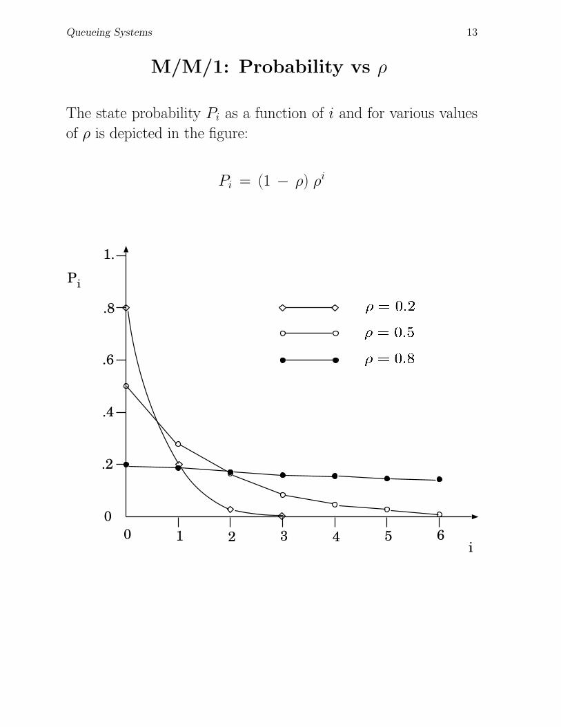
M/M/1: Probability vs ρ
The state probability Pi as a function of i and for various values
of ρ is depicted in the figure:
Pi = (1 − ρ) ρi
0
.2
.4
.6
.8
1.
0 1 2 3 4 5 6i
P i
������� �
����� �
������ �
Queueing Systems 14
Expected number of customers in a M/M/1
Server utilization factor (probability the server is busy):
U0 =∞∑i=1
Pi = 1 − P0 = ρ
Expected number of customers E[N ]
Let N be the number of customers in the queue, including the one
in service: the expected number of customers E[N ] is given by:
E[N ] =∞∑i=0
i · Pi
= 0 · P0 + 1 · ρ · P0 + 2 · ρ2 · P0 + 3 · ρ3 · P0 + . . .
= P0
∞∑i=0
i · ρi = (1− ρ)∞∑i=0
i · ρi =ρ
1− ρ
The above proof is based on the sum of the modified geometric
series:
∞∑i=0
i · ρi = ρ∂
∂ ρ
∞∑i=0
ρi = ρ∂
∂ ρ
1
1− ρ
=ρ
(1− ρ)2
Queueing Systems 15
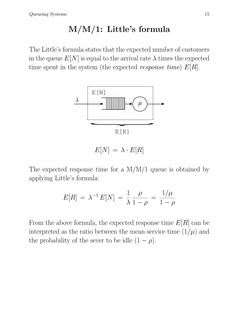
M/M/1: Little’s formula
The Little’s formula states that the expected number of customers
in the queue E[N ] is equal to the arrival rate λ times the expected
time spent in the system (the expected response time) E[R].
� � {E[N]
E[R]
E[N ] = λ · E[R]
The expected response time for a M/M/1 queue is obtained by
applying Little’s formula:
E[R] = λ−1 E[N ] =1
λ
ρ
1− ρ=
1/µ
1− ρ
From the above formula, the expected response time E[R] can be
interpreted as the ratio between the mean service time (1/µ) and
the probability of the sever to be idle (1− ρ).
Queueing Systems 16
M/M/1: Performance measures
Expected waiting time
Let us define the waiting time W = R−S as the time a customer
waits in the queue before service, where R is the response time
and S the service time.
The expected waiting time E[W ] is given by:
E[W ] = E[R] − E[S] =1
µ (1− ρ)− 1
µ=
ρ
µ (1− ρ)
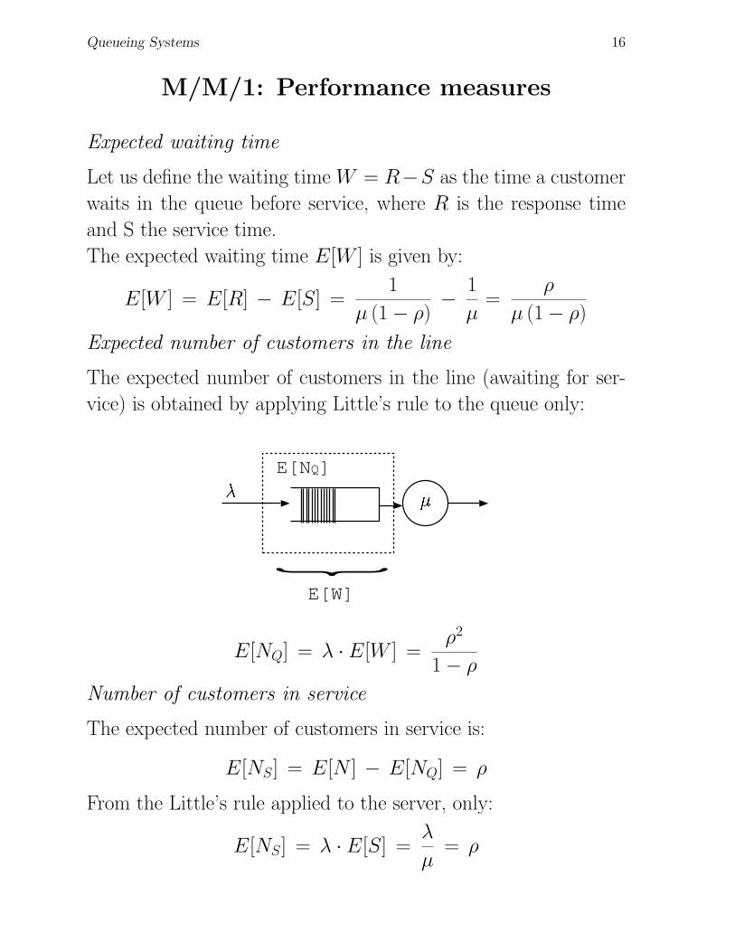
Expected number of customers in the line
The expected number of customers in the line (awaiting for ser-
vice) is obtained by applying Little’s rule to the queue only:
� �
{E[NQ]
E[W]
E[NQ] = λ · E[W ] =ρ2
1− ρ
Number of customers in service
The expected number of customers in service is:
E[NS] = E[N ] − E[NQ] = ρ
From the Little’s rule applied to the server, only:
E[NS] = λ · E[S] =λ
µ= ρ
Queueing Systems 17
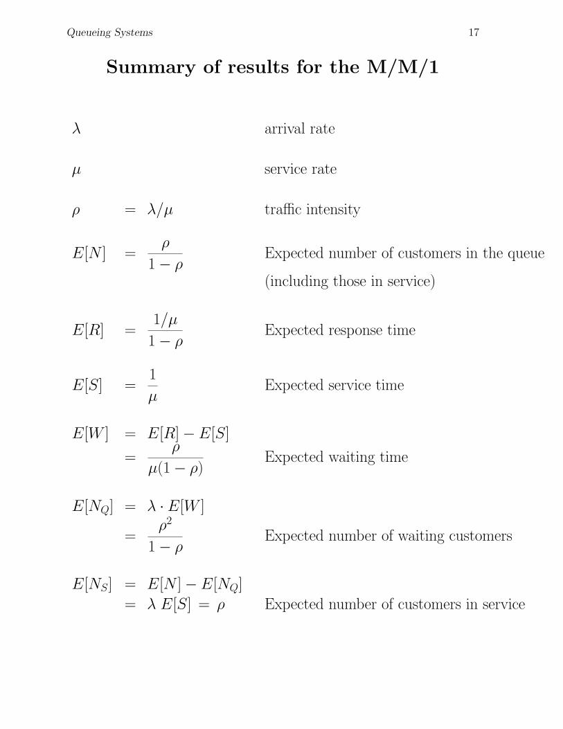
Summary of results for the M/M/1
λ arrival rate
µ service rate
ρ = λ/µ traffic intensity
E[N ] =ρ
1− ρExpected number of customers in the queue
(including those in service)
E[R] =1/µ
1− ρExpected response time
E[S] =1
µExpected service time
E[W ] = E[R]− E[S]
=ρ
µ(1− ρ)Expected waiting time
E[NQ] = λ · E[W ]
=ρ2
1− ρExpected number of waiting customers
E[NS] = E[N ]− E[NQ]
= λ E[S] = ρ Expected number of customers in service
Queueing Systems 18
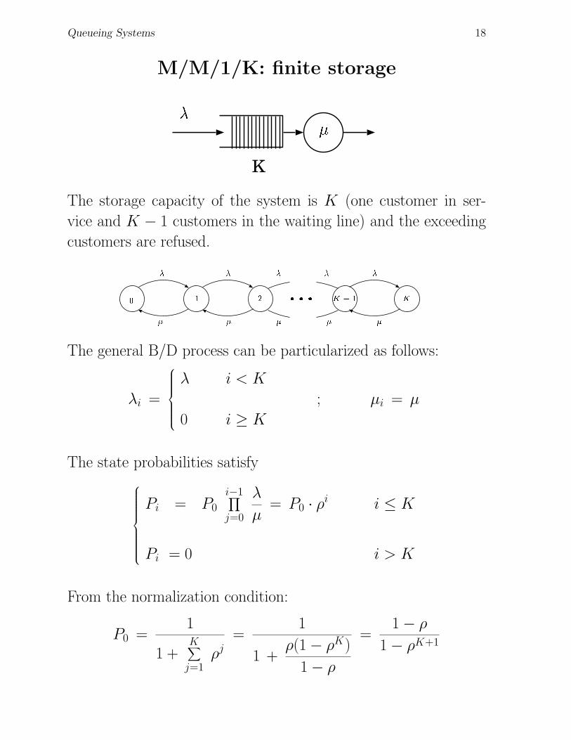
M/M/1/K: finite storage
�
�
K
The storage capacity of the system is K (one customer in ser-
vice and K − 1 customers in the waiting line) and the exceeding
customers are refused.
�
�
� � �
� � � �
� �
� � ����� �
The general B/D process can be particularized as follows:
λi =
λ i < K
; µi = µ
0 i ≥ K
The state probabilities satisfy
Pi = P0
i−1∏
j=0
λ
µ= P0 · ρi i ≤ K
Pi = 0 i > K
From the normalization condition:
P0 =1
1 +K∑
j=1ρj
=1
1 +ρ(1− ρK)
1− ρ
=1− ρ
1− ρK+1
Queueing Systems 19
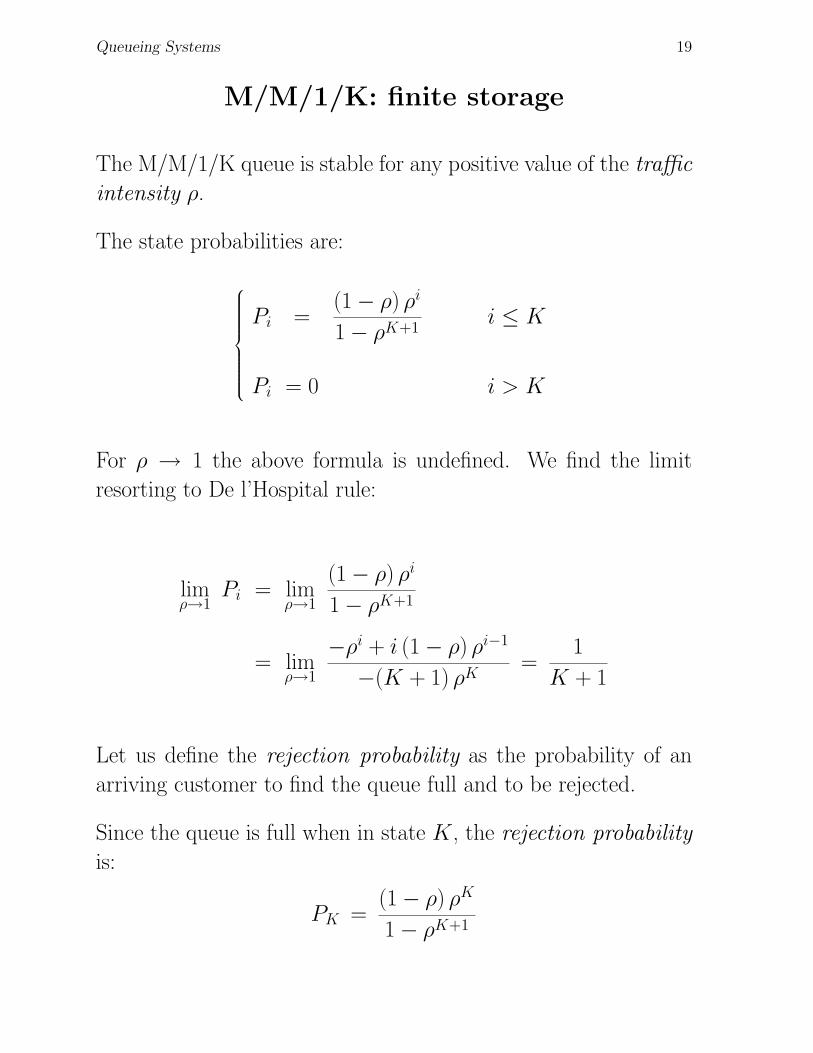
M/M/1/K: finite storage
The M/M/1/K queue is stable for any positive value of the traffic
intensity ρ.
The state probabilities are:
Pi =(1− ρ) ρi
1− ρK+1i ≤ K
Pi = 0 i > K
For ρ → 1 the above formula is undefined. We find the limit
resorting to De l’Hospital rule:
limρ→1
Pi = limρ→1
(1− ρ) ρi
1− ρK+1
= limρ→1
−ρi + i (1− ρ) ρi−1
−(K + 1) ρK=
1
K + 1
Let us define the rejection probability as the probability of an
arriving customer to find the queue full and to be rejected.
Since the queue is full when in state K, the rejection probability
is:
PK =(1− ρ) ρK
1− ρK+1
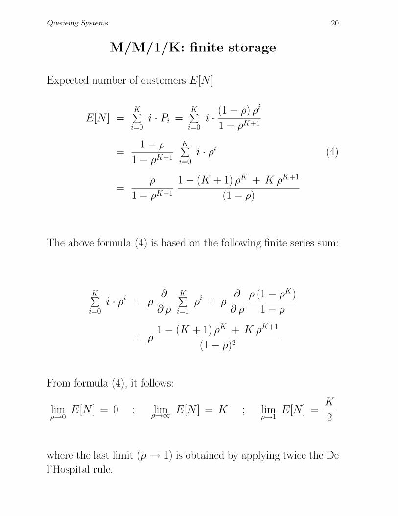
Queueing Systems 20
M/M/1/K: finite storage
Expected number of customers E[N ]
E[N ] =K∑
i=0i · Pi =
K∑
i=0i · (1− ρ) ρi
1− ρK+1
=1− ρ
1− ρK+1
K∑
i=0i · ρi (4)
=ρ
1− ρK+1
1− (K + 1) ρK + K ρK+1
(1− ρ)
The above formula (4) is based on the following finite series sum:
K∑
i=0i · ρi = ρ
∂
∂ ρ
K∑
i=1ρi = ρ
∂
∂ ρ
ρ (1− ρK)
1− ρ
= ρ1− (K + 1) ρK + K ρK+1
(1− ρ)2
From formula (4), it follows:
limρ→0
E[N ] = 0 ; limρ→∞ E[N ] = K ; lim
ρ→1E[N ] =
K
2
where the last limit (ρ → 1) is obtained by applying twice the De
l’Hospital rule.
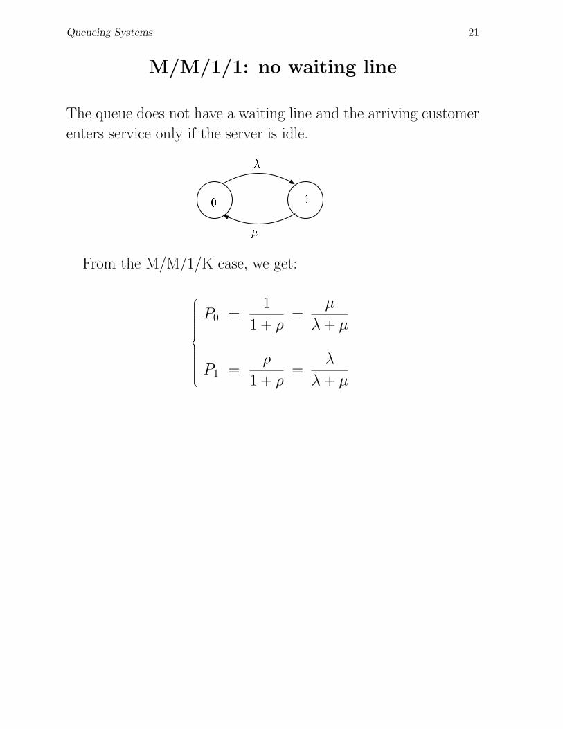
Queueing Systems 21
M/M/1/1: no waiting line
The queue does not have a waiting line and the arriving customer
enters service only if the server is idle.
�
�
� �
From the M/M/1/K case, we get:
P0 =1
1 + ρ=
µ
λ + µ
P1 =ρ
1 + ρ=
λ
λ + µ
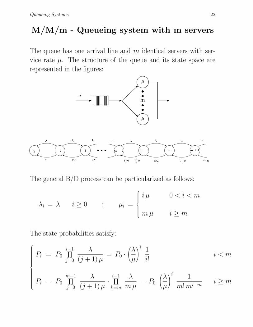
Queueing Systems 22
M/M/m - Queueing system with m servers
The queue has one arrival line and m identical servers with ser-
vice rate µ. The structure of the queue and its state space are
represented in the figures:
�
�
�
m
�
�
� � �
� � � �
� �� �����������
����� ��� � !�"$#
%
&('
) *�+-,
. /
0(1 2(3
The general B/D process can be particularized as follows:
λi = λ i ≥ 0 ; µi =
i µ 0 < i < m
mµ i ≥ m
The state probabilities satisfy:
Pi = P0
i−1∏
j=0
λ
(j + 1) µ= P0 ·
λ
µ
i 1
i!i < m
Pi = P0
m−1∏
j=0
λ
(j + 1) µ· i−1∏
k=m
λ
mµ= P0
λ
µ
i 1
m! mi−mi ≥ m
Queueing Systems 23
M/M/m - Queueing system with m servers
Let us define the traffic intensity as ρ =λ
mµ.
The stability condition requires ρ < 1.
By rewriting the state probabilities in terms of the traffic intensity,
we obtain:
Pi =
P0(mρ)i
i !i < m
P0ρi mm
m!i ≥ m
From the normalization condition, we obtain:
P0 =
m−1∑
i=0
(mρ)i
i !+
∞∑i=m
ρi mm
m!
−1
(5)
The second sum in (5) can be written as:
∞∑i=m
ρi mm
m!=
ρm mm
m !
∞∑k=0
ρk =(mρ)m
m !
1
1− ρ
So that (5) becomes:
P0 =
m−1∑
i=0
(mρ)i
i !+
(mρ)m
m !
1
1− ρ
−1
Queueing Systems 24
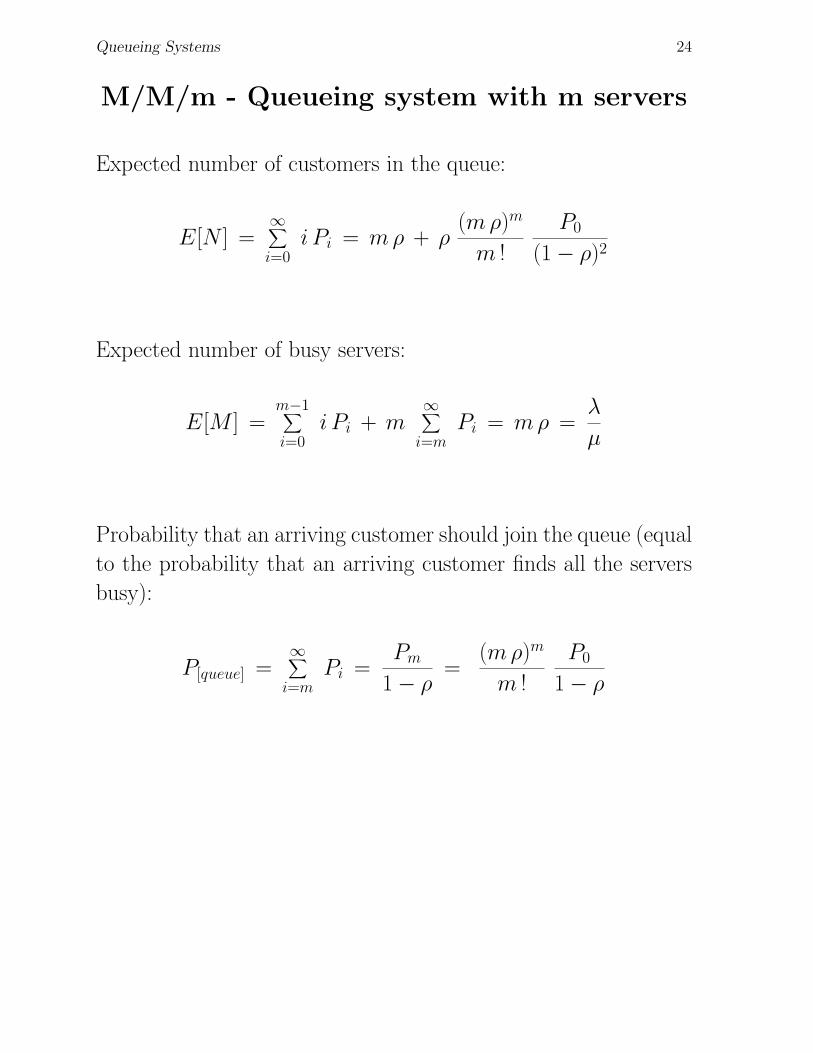
M/M/m - Queueing system with m servers
Expected number of customers in the queue:
E[N ] =∞∑i=0
i Pi = mρ + ρ(mρ)m
m !
P0
(1− ρ)2
Expected number of busy servers:
E[M ] =m−1∑
i=0i Pi + m
∞∑i=m
Pi = mρ =λ
µ
Probability that an arriving customer should join the queue (equal
to the probability that an arriving customer finds all the servers
busy):
P[queue] =∞∑
i=mPi =
Pm
1− ρ=
(mρ)m
m !
P0
1− ρ
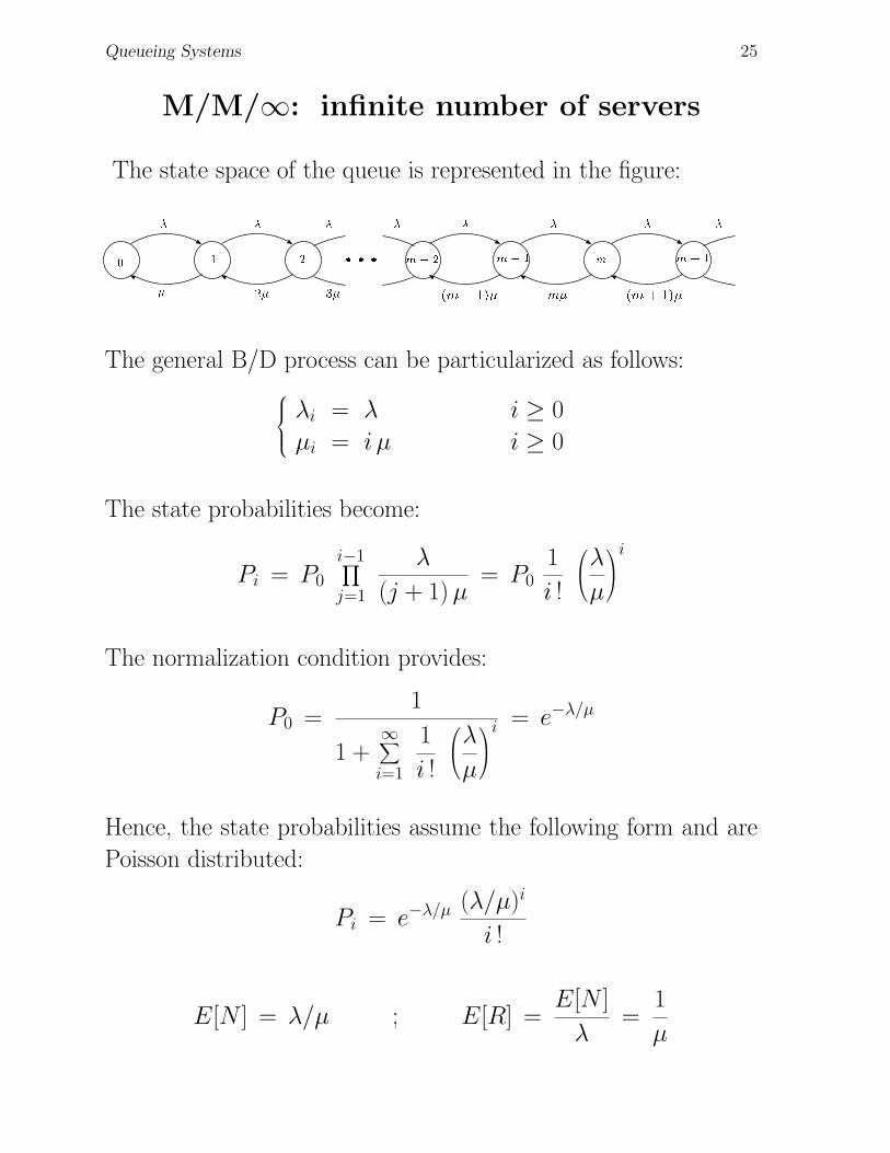
Queueing Systems 25
M/M/∞: infinite number of servers
The state space of the queue is represented in the figure:
�
�
� � �
� � � �
� �� �����������
����� ��� � !�"$#
%
&('
) *�+-,
. /
0�13254�6�7
The general B/D process can be particularized as follows:
λi = λ i ≥ 0
µi = i µ i ≥ 0
The state probabilities become:
Pi = P0
i−1∏
j=1
λ
(j + 1) µ= P0
1
i !
λ
µ
i
The normalization condition provides:
P0 =1
1 +∞∑i=1
1
i !
λ
µ
i = e−λ/µ
Hence, the state probabilities assume the following form and are
Poisson distributed:
Pi = e−λ/µ (λ/µ)i
i !
E[N ] = λ/µ ; E[R] =E[N ]
λ=
1
µ


![Research Paper Disease-specific ... - Journal of Cancer · Lung cancer is the leading cause of cancer-death for men and the second cause of cancer-death for women worldwide [1]. In](https://static.fdocument.org/doc/165x107/5ec819717980846d715bda4b/research-paper-disease-specific-journal-of-cancer-lung-cancer-is-the-leading.jpg)
![ΠΑΝΕΠΙΣΤΗΜΙΟ ΑΙΓΑΙΟΥ · Sennott L.I. (1999) Stochastic Dynamic Programming and the Control of Queueing Systems, Wiley, New York. [4]. Tijms H.C. (2003) A First](https://static.fdocument.org/doc/165x107/5f65698502aee000925f8724/oe-sennott-li-1999-stochastic-dynamic-programming.jpg)