Bayesian Optimization with Exponential Convergence

Kenji KawaguchiMIT

Cambridge, MA, 02139kawaguch@mit.edu

Leslie Pack KaelblingMIT

Cambridge, MA, 02139lpk@csail.mit.edu

Tomas Lozano-PerezMIT

Cambridge, MA, 02139tlp@csail.mit.edu

Abstract

This paper presents a Bayesian optimization method with exponential conver-gencewithout the need of auxiliary optimization andwithout the δ-cover sam-pling. Most Bayesian optimization methods require auxiliary optimization: an ad-ditional non-convex global optimization problem, which can be time-consumingand hard to implement in practice. Also, the existing Bayesian optimizationmethod with exponential convergence [1] requires access to theδ-cover sampling,which was considered to be impractical [1, 2]. Our approach eliminates both re-quirements and achieves an exponential convergence rate.

1 Introduction

We consider a general global optimization problem: maximizef(x) subject tox ∈ Ω ⊂ RD wheref : Ω → R is a non-convex black-box deterministic function. Such a problem arises in many real-world applications, such as parameter tuning in machine learning [3], engineering design problems[4], and model parameter fitting in biology [5]. For this problem, one performance measure of analgorithm is thesimple regret, rn, which is given byrn = supx∈Ω f(x) − f(x+) wherex+ is thebest input vector found by the algorithm. For brevity, we use the term “regret” to mean simple regret.

The general global optimization problem is known to be intractable if we make no further assump-tions [6]. The simplest additional assumption to restore tractability is to assume the existence of abound on the slope off . A well-known variant of this assumption is Lipschitz continuity with aknown Lipschitz constant, and many algorithms have been proposed in this setting [7, 8, 9]. Thesealgorithms successfully guaranteed certain bounds on the regret. However appealing from a theoret-ical point of view, a practical concern was soon raised regarding the assumption that a tight Lipschitzconstant is known. Some researchers relaxed this somewhat strong assumption by proposing proce-dures to estimate a Lipschitz constant during the optimization process [10, 11, 12].

Bayesian optimization is an efficient way to relax this assumption of complete knowledge of the Lip-schitz constant, and has become a well-recognized method for solving global optimization problemswith non-convex black-box functions. In the machine learning community, Bayesian optimization—especially by means of a Gaussian process (GP)—is an active research area [13, 14, 15]. With therequirement of the access to theδ-cover sampling procedure (it samples the function uniformly suchthat the density of samples doubles in the feasible regions at each iteration), de Freitas et al. [1] re-cently proposed a theoretical procedure that maintains an exponential convergence rate (exponentialregret). However, as pointed out by Wang et al. [2], one remaining problem is to derive a GP-basedoptimization method with an exponential convergence ratewithout theδ-cover sampling procedure,which is computationally too demanding in many cases.

In this paper, we propose a novel GP-based global optimization algorithm, which maintains anexponential convergence rate and converges rapidlywithout theδ-cover sampling procedure.

1

2 Gaussian Process Optimization

In Gaussian process optimization, we estimate the distribution over functionf and use this informa-tion to decide which point off should be evaluated next. In a parametric approach, we consider a pa-rameterized functionf(x; θ), with θ being distributed according to some prior. In contrast, the non-parametric GP approach directly puts the GP prior overf asf(∙) ∼ GP (m(∙), κ(∙, ∙)) wherem(∙) isthe mean function andκ(∙, ∙) is the covariance function or the kernel. That is,m(x) = E[f(x)] andκ(x, x′) = E[(f(x)−m(x))(f(x′)−m(x′))T ]. For a finite set of points, the GP model is simply ajoint Gaussian:f(x1:N ) ∼ N (m(x1:N ),K), whereKi,j = κ(xi, xj) andN is the number of datapoints. To predict the value off at a new data point, we first consider the joint distribution overfof the old data points and the new data point:

(f(x1:N )f(xN+1)

)

∼ N

(m(x1:N )m(xN+1)

,

[K k

kT κ(xN+1, xN+1)

])

wherek = κ(x1:N ,xN+1) ∈ RN×1. Then, after factorizing the joint distribution using the Schurcomplement for the joint Gaussian, we obtain the conditional distribution, conditioned on observedentitiesDN := {x1:N , f(x1:N )} andxN+1, as:

f(xN+1)|DN , xN+1 ∼ N (μ(xN+1|DN ), σ2(xN+1|DN ))

where μ(xN+1|DN ) = m(xN+1) + kT K−1(f(x1:N ) − m(x1:N )) and σ2(xN+1|DN ) =κ(xN+1,xN+1) − kT K−1k. One advantage of GP is that this closed-form solution simplifies bothits analysis and implementation.

To use a GP, we must specify the mean function and the covariance function. The mean function isusually set to be zero. With this zero mean function, the conditional meanμ(xN+1|DN ) can stillbe flexibly specified by the covariance function, as shown in the above equation forμ. For the co-variance function, there are several common choices, including the Matern kernel and the Gaussian

kernel. For example, the Gaussian kernel is defined asκ(x, x′) = exp(− 1

2 (x − x′)T Σ−1(x − x′))

whereΣ−1 is the kernel parameter matrix. The kernel parameters or hyperparameters can be esti-mated by empirical Bayesian methods [16]; see [17] for more information about GP.

The flexibility and simplicity of the GP prior make it a common choice for continuous objectivefunctions in the Bayesian optimization literature. Bayesian optimization with GP selects the nextquery point that optimizes the acquisition function generated by GP. Commonly used acquisitionfunctions include the upper confidence bound (UCB) and expected improvement (EI). For brevity,we consider Bayesian optimization with UCB, which works as follows. At each iteration, the UCBfunctionU is maintained asU(x|DN ) = μ(x|DN ) + ςσ(x|DN ) whereς ∈ R is a parameter of thealgorithm. To find the next queryxn+1 for the objective functionf , GP-UCB solves an additionalnon-convex optimization problem withU asxN+1 = arg maxx U(x|DN ). This is often carried outby other global optimization methods such as DIRECT and CMA-ES. The justification for intro-ducing a new optimization problem lies in the assumption that the cost of evaluating the objectivefunctionf dominates that of solving additional optimization problem.

For deterministic function, de Freitas et al. [1] recently presented a theoretical procedure that main-tains exponential convergence rate. However, their own paper and the follow-up research [1, 2] pointout that this result relies on an impractical sampling procedure, theδ-cover sampling. To overcomethis issue, Wang et al. [2] combined GP-UCB with a hierarchical partitioning optimization method,the SOO algorithm [18], providing a regret bound with polynomial dependence on the number offunction evaluations. They concluded that creating a GP-based algorithm with anexponentialcon-vergence ratewithout the impractical sampling procedure remained an open problem.

3 Infinite-Metric GP Optimization3.1 Overview

The GP-UCB algorithm can be seen as a member of the class of bound-based search methods,which includes Lipschitz optimization, A* search, and PAC-MDP algorithms with optimism in theface of uncertainty. Bound-based search methods have a common property: the tightness of thebound determines its effectiveness. The tighter the bound is, the better the performance becomes.

2

However, it is often difficult to obtain a tight bound while maintaining correctness. For example,in A* search, admissible heuristics maintain the correctness of the bound, but the estimated boundwith admissibility is often too loose in practice, resulting in a long period of global search.

The GP-UCB algorithm has the same problem. The bound in GP-UCB is represented by UCB,which has the following property:f(x) ≤ U(x|D) with some probability. We formalize this prop-erty in the analysis of our algorithm. The problem is essentially due to the difficulty of obtaining atight boundU(x|D) such thatf(x) ≤ U(x|D) andf(x) ≈ U(x|D) (with some probability). Oursolution strategy is to first admit that the bound encoded in GP prior may not be tight enough to beuseful by itself. Instead of relying on a single bound given by the GP, we leverage the existence ofanunknownbound encoded in the continuity at a global optimizer.

Assumption 1. (Unknown Bound) There exists a global optimizerx∗ and anunknownsemi-metric` such that for allx ∈ Ω, f(x∗) ≤ f(x) + ` (x, x∗) and` (x, x∗) < ∞.

In other words, we do not expect theknownupper bound due to GP to be tight, but instead expect thatthere exists someunknownbound that might be tighter. Notice that in the case where the bound byGP is as tight as the unknown bound by semi-metric` in Assumption 1, our method still maintains anexponential convergence rate and an advantage over GP-UCB (no need for auxiliary optimization).Our method is expected to become relatively much better when theknownbound due to GP is lesstight compared to the unknown bound by`.

As the semi-metric is unknown, there are infinitely many possible candidates that we can think offor `. Accordingly, we simultaneously conduct global and local searches based on all the candidatesof the bounds. The bound estimated by GP is used to reduce the number of candidates. Sincethe bound estimated by GP is known, we can ignore the candidates of the bounds that are looserthan the bound estimated by GP. The source code of the proposed algorithm is publicly available athttp://lis.csail.mit.edu/code/imgpo.html .

3.2 Description of Algorithm

Figure 1 illustrates how the algorithm works with a simple 1-dimensional objective function. Weemploy hierarchical partitioning to maintain hyperintervals, as illustrated by the line segments in thefigure. We consider a hyperrectangle as our hyperinterval, with its center being the evaluation pointof f (blue points in each line segment in Figure 1). For each iterationt, the algorithm performs thefollowing procedurefor each interval size:

(i) Select the interval with the maximum center value among the intervals of the same size.(ii) Keep the interval selected by (i) if it has a center value greater than that of anylarger

interval.(iii) Keep the interval accepted by (ii) if it contains a UCB greater than the center value of any

smallerinterval.(iv) If an interval is accepted by (iii), divide it along with the longest coordinate into three new

intervals.(v) For each new interval, if the UCB of the evaluation point is less than the best function value

found so far, skip the evaluation and use the UCB value as the center value until the intervalis accepted in step (ii) on some future iteration; otherwise, evaluate the center value.

(vi) Repeat steps (i)–(v) until every size of intervals are considered

Then, at the end of each iteration, the algorithm updates the GP hyperparameters. Here, the purposeof steps (i)–(iii) is to select an interval that might contain the global optimizer. Steps (i) and (ii)select the possible intervals based on the unknown bound by`, while Step (iii) does so based on thebound by GP.

We now explain the procedure using the example in Figure 1. Letn be the number of divisions ofintervals and letN be the number of function evaluations.t is the number of iterations. Initially,there is only one interval (the center of the input regionΩ ⊂ R) and thus this interval is divided,resulting in the first diagram of Figure 1. At the beginning of iterationt = 2 , step (i) selects the thirdinterval from the left side in the first diagram (t = 1, n = 2), as its center value is the maximum.Because there are no intervals of different size at this point, steps (ii) and (iii) are skipped. Step(iv) divides the third interval, and then the GP hyperparameters are updated, resulting in the second

3

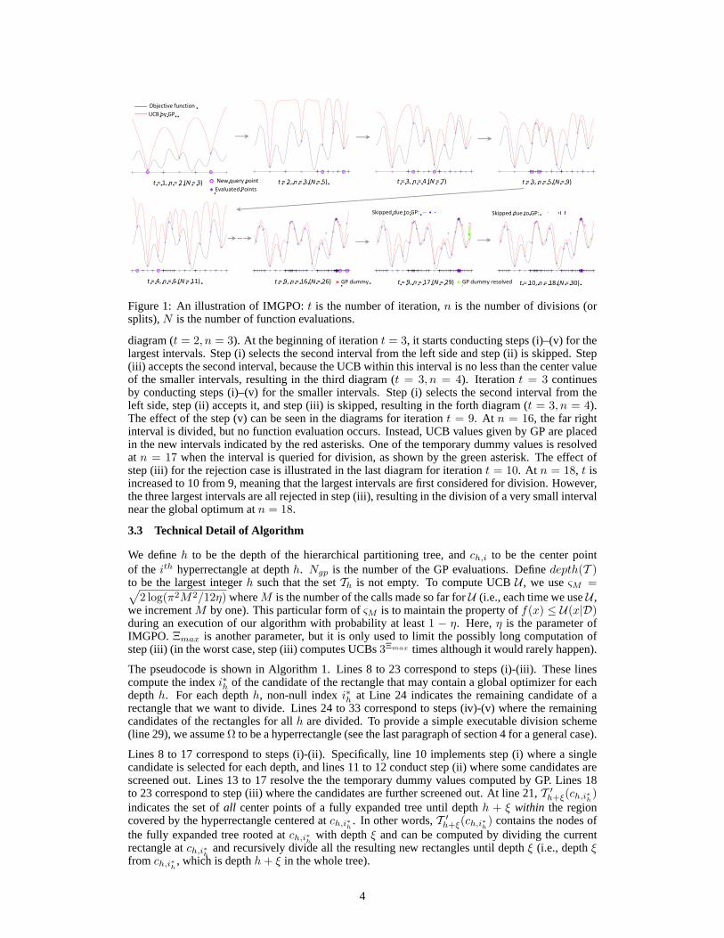
Figure 1: An illustration of IMGPO:t is the number of iteration,n is the number of divisions (orsplits),N is the number of function evaluations.

diagram (t = 2, n = 3). At the beginning of iterationt = 3, it starts conducting steps (i)–(v) for thelargest intervals. Step (i) selects the second interval from the left side and step (ii) is skipped. Step(iii) accepts the second interval, because the UCB within this interval is no less than the center valueof the smaller intervals, resulting in the third diagram (t = 3, n = 4). Iterationt = 3 continuesby conducting steps (i)–(v) for the smaller intervals. Step (i) selects the second interval from theleft side, step (ii) accepts it, and step (iii) is skipped, resulting in the forth diagram (t = 3, n = 4).The effect of the step (v) can be seen in the diagrams for iterationt = 9. At n = 16, the far rightinterval is divided, but no function evaluation occurs. Instead, UCB values given by GP are placedin the new intervals indicated by the red asterisks. One of the temporary dummy values is resolvedat n = 17 when the interval is queried for division, as shown by the green asterisk. The effect ofstep (iii) for the rejection case is illustrated in the last diagram for iterationt = 10. At n = 18, t isincreased to 10 from 9, meaning that the largest intervals are first considered for division. However,the three largest intervals are all rejected in step (iii), resulting in the division of a very small intervalnear the global optimum atn = 18.

3.3 Technical Detail of Algorithm

We defineh to be the depth of the hierarchical partitioning tree, andch,i to be the center pointof the ith hyperrectangle at depthh. Ngp is the number of the GP evaluations. Definedepth(T )to be the largest integerh such that the setTh is not empty. To compute UCBU , we useςM =√

2 log(π2M2/12η) whereM is the number of the calls made so far forU (i.e., each time we useU ,we incrementM by one). This particular form ofςM is to maintain the property off(x) ≤ U(x|D)during an execution of our algorithm with probability at least1 − η. Here,η is the parameter ofIMGPO. Ξmax is another parameter, but it is only used to limit the possibly long computation ofstep (iii) (in the worst case, step (iii) computes UCBs3Ξmax times although it would rarely happen).

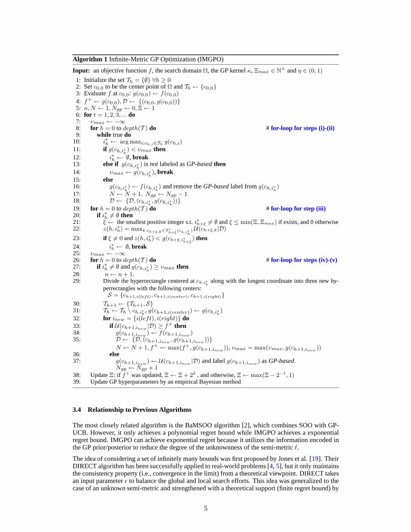
The pseudocode is shown in Algorithm 1. Lines 8 to 23 correspond to steps (i)-(iii). These linescompute the indexi∗h of the candidate of the rectangle that may contain a global optimizer for eachdepthh. For each depthh, non-null indexi∗h at Line 24 indicates the remaining candidate of arectangle that we want to divide. Lines 24 to 33 correspond to steps (iv)-(v) where the remainingcandidates of the rectangles for allh are divided. To provide a simple executable division scheme(line 29), we assumeΩ to be a hyperrectangle (see the last paragraph of section 4 for a general case).

Lines 8 to 17 correspond to steps (i)-(ii). Specifically, line 10 implements step (i) where a singlecandidate is selected for each depth, and lines 11 to 12 conduct step (ii) where some candidates arescreened out. Lines 13 to 17 resolve the the temporary dummy values computed by GP. Lines 18to 23 correspond to step (iii) where the candidates are further screened out. At line 21,T ′

h+ξ(ch,i∗h)

indicates the set ofall center points of a fully expanded tree until depthh + ξ within the regioncovered by the hyperrectangle centered atch,i∗h

. In other words,T ′h+ξ(ch,i∗h

) contains the nodes ofthe fully expanded tree rooted atch,i∗h

with depthξ and can be computed by dividing the currentrectangle atch,i∗h

and recursively divide all the resulting new rectangles until depthξ (i.e., depthξfrom ch,i∗h

, which is depthh + ξ in the whole tree).

4

Algorithm 1 Infinite-Metric GP Optimization (IMGPO)

Input: an objective functionf , the search domainΩ, the GP kernelκ, Ξmax ∈ N+ andη ∈ (0, 1)

1: Initialize the setTh = {∅} ∀h ≥ 02: Setc0,0 to be the center point ofΩ andT0 ← {c0,0}3: Evaluatef at c0,0: g(c0,0)← f(c0,0)

4: f+ ← g(c0,0),D ← {(c0,0, g(c0,0))}5: n, N ← 1, Ngp ← 0, Ξ← 16: for t = 1, 2, 3, ... do7: υmax ← −∞8: for h = 0 to depth(T ) do # for-loop for steps (i)-(ii)9: while truedo

10: i∗h ← arg maxi:ch,i∈Thg(ch,i)

11: if g(ch,i∗h) < υmax then

12: i∗h ← ∅, break13: else if g(ch,i∗h

) is not labeled asGP-basedthen14: υmax ← g(ch,i∗h

), break15: else16: g(ch,i∗h

)← f(ch,i∗h) and remove theGP-basedlabel fromg(ch,i∗h

)

17: N ← N + 1, Ngp ← Ngp − 118: D ← {D, (ch,i∗h

, g(ch,i∗h))}

19: for h = 0 to depth(T ) do # for-loop for step (iii)20: if i∗h 6= ∅ then21: ξ ← the smallest positive integer s.t.i∗h+ξ 6= ∅ andξ ≤ min(Ξ, Ξmax) if exists, and 0 otherwise22: z(h, i∗h) = maxk:ch+ξ,k∈T ′

h+ξ(ch,i∗

h) U(ch+ξ,k|D)

23: if ξ 6= 0 andz(h, i∗h) < g(ch+ξ,i∗h+ξ

) then24: i∗h ← ∅, break25: υmax ← −∞26: for h = 0 to depth(T ) do # for-loop for steps (iv)-(v)27: if i∗h 6= ∅ andg(ch,i∗h

) ≥ υmax then28: n← n + 1.29: Divide the hyperrectangle centered atch,i∗

halong with the longest coordinate into three new hy-

perrectangles with the following centers:S = {ch+1,i(left), ch+1,i(center), ch+1,i(right)}

30: Th+1 ← {Th+1,S}31: Th ← Th \ ch,i∗h

, g(ch+1,i(center))← g(ch,i∗h)

32: for inew = {i(left), i(right)} do33: if U(ch+1,inew

|D) ≥ f+ then34: g(ch+1,inew

)← f(ch+1,inew)

35: D ← {D, (ch+1,inew, g(ch+1,inew

))}N ← N + 1, f+ ← max(f+, g(ch+1,inew

)), υmax = max(υmax, g(ch+1,inew))

36: else37: g(ch+1,inew

)← U(ch+1,inew|D) and labelg(ch+1,inew

) asGP-based.Ngp ← Ngp + 1

38: UpdateΞ: if f+ was updated,Ξ← Ξ + 22 , and otherwise,Ξ← max(Ξ− 2−1, 1)39: Update GP hyperparameters by an empirical Bayesian method

3.4 Relationship to Previous Algorithms

The most closely related algorithm is the BaMSOO algorithm [2], which combines SOO with GP-UCB. However, it only achieves a polynomial regret bound while IMGPO achieves a exponentialregret bound. IMGPO can achieve exponential regret because it utilizes the information encoded inthe GP prior/posterior to reduce the degree of the unknownness of the semi-metric`.

The idea of considering a set of infinitely many bounds was first proposed by Jones et al. [19]. TheirDIRECT algorithm has been successfully applied to real-world problems [4, 5], but it only maintainsthe consistency property (i.e., convergence in the limit) from a theoretical viewpoint. DIRECT takesan input parameterε to balance the global and local search efforts. This idea was generalized to thecase of an unknown semi-metric and strengthened with a theoretical support (finite regret bound) by

5

Munos [18] in the SOO algorithm. By limiting the depth of the search tree with a parameterhmax,the SOO algorithm achieves a finite regret bound that depends onthe near-optimality dimension.

4 Analysis

In this section, we prove an exponential convergence rate of IMGPO and theoretically discuss thereason why the novel idea underling IMGPO is beneficial. The proofs are provided in the supple-mentary material. To examine the effect of considering infinitely many possible candidates of thebounds, we introduce the following term.

Definition 1. (Infinite-metric exploration loss). The infinite-metric exploration lossρt is the numberof intervals to be divided during iterationt.

The infinite-metric exploration lossρτ can be computed asρt =∑depth(T )

h=1 1(i∗h 6= ∅) at line25. It is the cost (in terms of the number of function evaluations) incurred by not committing toany particular upper bound. If we were to rely on a specific bound,ρτ would be minimized to 1.For example, the DOO algorithm [18] hasρt = 1 ∀t ≥ 1. Even if we know a particular upperbound, relying on this knowledge and thus minimizingρτ is not a good optionunless the knownbound is tight enough compared to the unknown bound leveraged in our algorithm. This will beclarified in our analysis. Letρt be the maximum of the averages ofρ1:t′ for t′ = 1, 2, ..., t (i.e.,

ρt ≡ max({ 1t′

∑t′

τ=1 ρτ ; t′ = 1, 2, ..., t}).

Assumption 2. There existL > 0, α > 0 andp ≥ 1 in R such that for allx, x′ ∈ Ω, `(x′, x) ≤L||x′ − x||αp .

In Theorem 1, we show that the exponential convergence rateO(λN+Ngp

)with λ < 1 is achieved.

We defineΞn ≤ Ξmax to be the largestξ used so far withn total node expansions. For simplicity,we assume thatΩ is a square, which we satisfied in our experiments by scaling originalΩ.

Theorem 1.Assume Assumptions 1 and 2. Letβ = supx,x′∈Ω12‖x−x′‖∞. Letλ = 3−

α2CDρt < 1.

Then, with probability at least1 − η, the regret of IMGPO is bounded as

rN ≤ L(3βD1/p)α exp

(

−α

[N + Ngp

2CDρt− Ξn − 2

]

ln 3

)

= O(λN+Ngp

).

Importantly, our bound holds for the best values of the unknownL,α and p even though thesevalues are not given. The closest result in previous work is that of BaMSOO [2], which obtainedO(n− 2α

D(4−α) ) with probability1 − η for α = {1, 2}. As can be seen, we have improved the regretbound. Additionally, in our analysis, we can see howL, p, andα affect the bound, allowing usto view the inherent difficulty of an objective function in a theoretical perspective. Here,C is aconstant inN and is used in previous work [18, 2]. For example, if we conduct2D or 3D − 1function evaluations per node-expansion and ifp = ∞, we have thatC = 1.

We note thatλ can get close to one as input dimensionD increases, which suggests that thereis a remaining challenge in scalability for higher dimensionality. One strategy for addressing thisproblem would be to leverage additional assumptions such as those in [14, 20].

Remark 1. (The effect of the tightness of UCB by GP) If UCB computed by GP is “useful” such

thatN/ρt = Ω(N), then our regret bound becomesO(exp

(−N+Ngp

2CD α ln 3))

. If the bound due to

UCB by GP is too loose (and thus useless),ρt can increase up toO(N/t) (due toρt ≤∑t

i=1 i/t ≤

O(N/t)), resulting in the regret bound ofO(exp

(− t(1+Ngp/N)

2CD α ln 3))

, which can be bounded

by O(exp

(−N+Ngp

2CD max( 1√N

, tN )α ln 3

))1. This is still better than the known results.

Remark 2. (The effect of GP) Without the use of GP, our regret bound would be as follows:rN ≤L(3βD1/p)α exp(−α[ N

2CD1ρt−2] ln 3), whereρt ≤ ρt is the infinite-metric exploration loss without

1This can be done by limiting the depth of search tree asdepth(T ) = O(√

N). Our proof works with thisadditional mechanism, but results in the regret bound withN being replaced by

√N . Thus, if we assume to

have at least “not useless” UCBs such thatN/ρt = Ω(√

N), this additional mechanism can be disadvanta-geous. Accordingly, we do not adopt it in our experiments.

6

GP. Therefore, the use of GP reduces the regret bound by increasingNgp and decreasingρt, but maypotentially increase the bound by increasingΞn ≤ Ξ.

Remark 3. (The effect of infinite-metric optimization) To understand the effect of considering allthe possible upper bounds, we consider the case without GP. If we consider all the possible bounds,we have the regret boundL(3βD1/p)α exp(−α[ N

2CD1ρt− 2] ln 3) for the best unknownL, α andp.

For standard optimization with a estimated bound, we haveL′(3βD1/p′)α′

exp(−α′[ N2C′D

− 2] ln 3)for an estimatedL′, α′, andp′. By algebraic manipulation, considering all the possible bounds has

a better regret whenρ−1t ≥ 2CD

N ln 3α (( N2C′D − 2) ln 3α′

+2 ln 3α − ln L′(3βD1/p′)α′

L(3βD1/p)α ). For an intuitive

insight, we can simplify the above by assumingα′ = α andC ′ = C asρ−1t ≥ 1− Cc2D

N ln L′Dα/p′

LDα/p .BecauseL andp are the ones that achieve the lowest bound, the logarithm on the right-hand side isalways non-negative. Hence,ρt = 1 always satisfies the condition. WhenL′ andp′ are not tightenough, the logarithmic term increases in magnitude, allowingρt to increase. For example, if thesecond term on the right-hand side has a magnitude of greater than 0.5, thenρt = 2 satisfies theinequality. Therefore, even if we know the upper bound of the function, we can see that it may bebetter not to rely on this, but rather take the infinite many possibilities into account.

One may improve the algorithm with different division procedures than one presented in Algorithm1. Accordingly, in the supplementary material, we derive an abstract version of the regret bound forIMGPO with a family of division procedures that satisfy some assumptions. This information couldbe used to design a new division procedure.

5 ExperimentsIn this section, we compare the IMGPO algorithm with the SOO, BaMSOO, GP-PI and GP-EI algo-rithms [18, 2, 3]. In previous work, BaMSOO and GP-UCB were tested with a pair of a handpickedgood kernel and hyperparameters for each function [2]. In our experiments, we assume that theknowledge of good kernel and hyperparameters is unavailable, which is usually the case in practice.Thus, for IMGPO, BaMSOO, GP-PI and GP-EI, we simply used one of the most popular kernels,the isotropic Matern kernel withν = 5/2. This is given byκ(x, x′) = g(

√5||x − x′||2/l), where

g(z) = σ2(1 + z + z2/3) exp(−z). Then, we blindly initialized the hyperparameters toσ = 1

(a) Sin1: [1, 1.92, 2] (b) Sin2: [2, 3.37, 3] (c) Peaks: [2, 3.14, 4]

(d) Rosenbrock2: [2, 3.41, 4] (e) Branin: [2, 4.44, 2] (f) Hartmann3: [3, 4.11, 3]

(g) Hartmann6: [6, 4.39, 4] (h) Shekel5: [4, 3.95, 4] (i) Sin1000: [1000, 3.95, 4]

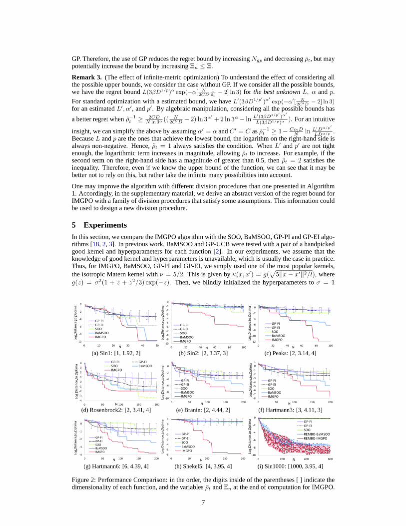
Figure 2: Performance Comparison: in the order, the digits inside of the parentheses [ ] indicate thedimensionality of each function, and the variablesρt andΞn at the end of computation for IMGPO.

7

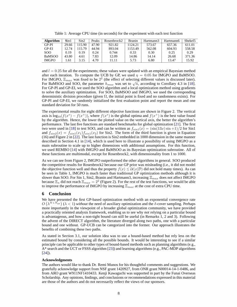
Table 1: Average CPU time (in seconds) for the experiment with each test function

Algorithm S in1 Sin2 Peaks Rosenbrock2 Branin Hartmann3 Hartmann6 Shekel5GP-PI 29.66 115.90 47.90 921.82 1124.21 573.67 657.36 611.01GP-EI 12.74 115.79 44.94 893.04 1153.49 562.08 604.93 558.58SOO 0.19 0.19 0.24 0.744 0.33 0.30 0.25 0.29BaMSOO 43.80 4.61 7.83 12.09 14.86 14.14 26.68 371.36IMGPO 1.61 3.15 4.70 11.11 5.73 6.80 13.47 15.92

andl = 0.25 for all the experiments; these values were updated with an empirical Bayesian methodafter each iteration. To compute the UCB by GP, we usedη = 0.05 for IMGPO and BaMSOO.For IMGPO,Ξmax was fixed to be22 (the effect of selecting different values is discussed later).For BaMSOO and SOO, the parameterhmax was set to

√n, according to Corollary 4.3 in [18].

For GP-PI and GP-EI, we used the SOO algorithm and a local optimization method using gradientsto solve the auxiliary optimization. For SOO, BaMSOO and IMGPO, we used the correspondingdeterministic division procedure (givenΩ, the initial point is fixed and no randomness exists). ForGP-PI and GP-EI, we randomly initialized the first evaluation point and report the mean and onestandard deviation for 50 runs.

The experimental results for eight different objective functions are shown in Figure 2. The verticalaxis is log10(f(x∗) − f(x+)), wheref(x∗) is the global optima andf(x+) is the best value foundby the algorithm. Hence, the lower the plotted value on the vertical axis, the better the algorithm’sperformance. The last five functions are standard benchmarks for global optimization [21]. The firsttwo were used in [18] to test SOO, and can be written asfsin1(x) = (sin(13x) sin+1)/2 for Sin1andfsin2(x) = fsin1(x1)fsin1(x2) for Sin2. The form of the third function is given in Equation(16) and Figure 2 in [22]. The last function is Sin2 embedded in 1000 dimension in the same mannerdescribed in Section 4.1 in [14], which is used here to illustrate a possibility of using IMGPO as amain subroutine to scale up to higher dimensions with additional assumptions. For this function,we used REMBO [14] with IMGPO and BaMSOO as its Bayesian optimization subroutine. All ofthese functions are multimodal, except for Rosenbrock2, with dimensionality from 1 to 1000.

As we can see from Figure 2, IMGPO outperformed the other algorithms in general. SOO producedthe competitive results for Rosenbrock2 because our GP prior was misleading (i.e., it did not modelthe objective function well and thus the propertyf(x) ≤ U(x|D) did not hold many times). As canbe seen in Table 1, IMGPO is much faster than traditional GP optimization methods although it isslower than SOO. For Sin 1, Sin2, Branin and Hartmann3, increasingΞmax does not affect IMGPObecauseΞn did not reachΞmax = 22 (Figure 2). For the rest of the test functions, we would be ableto improve the performance of IMGPO by increasingΞmax at the cost of extra CPU time.

6 ConclusionWe have presented the first GP-based optimization method with an exponential convergence rateO(λN+Ngp

)(λ < 1) without the need of auxiliary optimization and theδ-cover sampling. Perhaps

more importantly in the viewpoint of a broader global optimization community, we have provideda practically oriented analysis framework, enabling us to see whynot relying on a particular boundis advantageous, and how a non-tight bound can still be useful (in Remarks 1, 2 and 3). Followingthe advent of the DIRECT algorithm, the literature diverged along two paths, one with a particularbound and one without. GP-UCB can be categorized into the former. Our approach illustrates thebenefits of combining these two paths.

As stated in Section 3.1, our solution idea was to use a bound-based method but rely less on theestimated bound by considering all the possible bounds. It would be interesting to see if a similarprinciple can be applicable to other types of bound-based methods such as planning algorithms (e.g.,A* search and the UCT or FSSS algorithm [23]) and learning algorithms (e.g., PAC-MDP algorithms[24]).

AcknowledgmentsThe authors would like to thank Dr. Remi Munos for his thoughtful comments and suggestions. Wegratefully acknowledge support from NSF grant 1420927, from ONR grant N00014-14-1-0486, andfrom ARO grant W911NF1410433. Kenji Kawaguchi was supported in part by the Funai OverseasScholarship. Any opinions, findings, and conclusions or recommendations expressed in this materialare those of the authors and do not necessarily reflect the views of our sponsors.

8

References

[1] N. De Freitas, A. J. Smola, and M. Zoghi. Exponential regret bounds for Gaussian process bandits withdeterministic observations. InProceedings of the 29th International Conference on Machine Learning(ICML), 2012.

[2] Z. Wang, B. Shakibi, L. Jin, and N. de Freitas. Bayesian Multi-Scale Optimistic Optimization. InPro-ceedings of the 17th International Conference on Artificial Intelligence and Statistics (AISTAT), pages1005–1014, 2014.

[3] J. Snoek, H. Larochelle, and R. P. Adams. Practical Bayesian optimization of machine learning algo-rithms. InProceedings of Advances in Neural Information Processing Systems (NIPS), pages 2951–2959,2012.

[4] R. G. Carter, J. M. Gablonsky, A. Patrick, C. T. Kelley, and O. J. Eslinger. Algorithms for noisy problemsin gas transmission pipeline optimization.Optimization and engineering, 2(2):139–157, 2001.

[5] J. W. Zwolak, J. J. Tyson, and L. T. Watson. Globally optimised parameters for a model of mitotic controlin frog egg extracts.IEEE Proceedings-Systems Biology, 152(2):81–92, 2005.

[6] L. C. W. Dixon. Global optima without convexity. Numerical Optimisation Centre, Hatfield Polytechnic,1977.

[7] B. O. Shubert. A sequential method seeking the global maximum of a function.SIAM Journal onNumerical Analysis, 9(3):379–388, 1972.

[8] D. Q. Mayne and E. Polak. Outer approximation algorithm for nondifferentiable optimization problems.Journal of Optimization Theory and Applications, 42(1):19–30, 1984.

[9] R. H. Mladineo. An algorithm for finding the global maximum of a multimodal, multivariate function.Mathematical Programming, 34(2):188–200, 1986.

[10] R. G. Strongin. Convergence of an algorithm for finding a global extremum.Engineering Cybernetics,11(4):549–555, 1973.

[11] D. E. Kvasov, C. Pizzuti, and Y. D. Sergeyev. Local tuning and partition strategies for diagonal GOmethods.Numerische Mathematik, 94(1):93–106, 2003.

[12] S. Bubeck, G. Stoltz, and J. Y. Yu. Lipschitz bandits without the Lipschitz constant. InAlgorithmicLearning Theory, pages 144–158. Springer, 2011.

[13] J. Gardner, M. Kusner, K. Weinberger, and J. Cunningham. Bayesian Optimization with Inequality Con-straints. InProceedings of The 31st International Conference on Machine Learning (ICML), pages 937–945, 2014.

[14] Z. Wang, M. Zoghi, F. Hutter, D. Matheson, and N. De Freitas. Bayesian optimization in high dimensionsvia random embeddings. InProceedings of the Twenty-Third international joint conference on ArtificialIntelligence, pages 1778–1784. AAAI Press, 2013.

[15] N. Srinivas, A. Krause, M. Seeger, and S. M. Kakade. Gaussian Process Optimization in the BanditSetting: No Regret and Experimental Design. InProceedings of the 27th International Conference onMachine Learning (ICML), pages 1015–1022, 2010.

[16] K. P. Murphy.Machine learning: a probabilistic perspective. MIT press, page 521, 2012.

[17] C. E. Rasmussen and C. Williams.Gaussian Processes for Machine Learning. MIT Press, 2006.

[18] R. Munos. Optimistic optimization of deterministic functions without the knowledge of its smoothness.In Proceedings of Advances in neural information processing systems (NIPS), 2011.

[19] D. R. Jones, C. D. Perttunen, and B. E. Stuckman. Lipschitzian optimization without the Lipschitz con-stant.Journal of Optimization Theory and Applications, 79(1):157–181, 1993.

[20] K. Kandasamy, J. Schneider, and B. Poczos. High dimensional Bayesian optimisation and bandits viaadditive models.arXiv preprint arXiv:1503.01673, 2015.

[21] S. Surjanovic and D. Bingham. Virtual library of simulation experiments: Test functions and datasets.Retrieved November 30, 2014, fromhttp://www.sfu.ca/ ˜ ssurjano , 2014.

[22] D. B. McDonald, W. J. Grantham, W. L. Tabor, and M. J. Murphy. Global and local optimization us-ing radial basis function response surface models.Applied Mathematical Modelling, 31(10):2095–2110,2007.

[23] T. J. Walsh, S. Goschin, and M. L. Littman. Integrating Sample-Based Planning and Model-Based Re-inforcement Learning. InProceedings of the 24th AAAI conference on Artificial Intelligence (AAAI),2010.

[24] A. L. Strehl, L. Li, and M. L. Littman. Reinforcement learning in finite MDPs: PAC analysis.The Journalof Machine Learning Research (JMLR), 10:2413–2444, 2009.

9