Approximation by Conic Splines - University of...
31
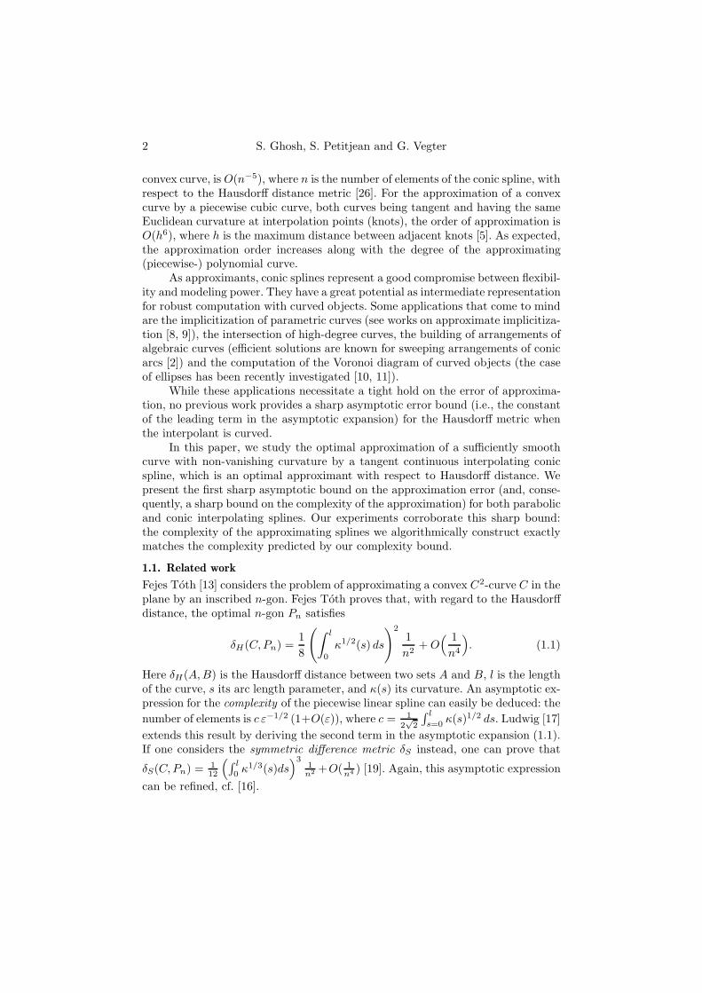
Approximation by Conic Splines Sunayana Ghosh, Sylvain Petitjean and Gert Vegter Abstract. We show that the complexity of a parabolic or conic spline approx- imating a sufficiently smooth curve with non-vanishing curvature to within Hausdorff distance ε is c1ε -1/4 + O(1), if the spline consists of parabolic arcs, and c2ε -1/5 + O(1), if it is composed of general conic arcs of varying type. The constants c1 and c2 are expressed in the Euclidean and affine curvature of the curve. We also show that the Hausdorff distance between a curve and an optimal conic arc tangent at its endpoints is increasing with its arc length, provided the affine curvature along the arc is monotone. This property yields a simple bisection algorithm for the computation of an optimal parabolic or conic spline. Mathematics Subject Classification (2000). Primary 65D07, 65D17; Secondary 68Q25. Keywords. Approximation, splines, conics, Hausdorff distance, complexity, dif- ferential geometry, affine curvature, affine spiral. 1. Introduction In the field of computer aided geometric design, one of the central topics is the approximation of complex geometric objects with simpler ones. An important part of this field concerns the approximation of plane curves and the asymptotic analysis of the rate of convergence of approximation schemes with respect to different metrics, the most commonly used being the Hausdorff metric. Various error bounds and convergence rates have been obtained for several types of (low-degree) approximation primitives. For the approximation of plane convex curves by polygons with n edges, the order of convergence is O(n -2 ) for several metrics, including the Hausdorff metric [13, 16, 17, 19]. When approximat- ing by a tangent continuous conic spline, the order of convergence, for a strictly The research of SG and GV was partially supported by grant 6413 of the European Commission to the IST-2002 FET-Open project Algorithms for Complex Shapes in the Sixth Framework Program.
Transcript of Approximation by Conic Splines - University of...
Approximation by Conic Splines
Sunayana Ghosh, Sylvain Petitjean and Gert Vegter
Abstract. We show that the complexity of a parabolic or conic spline approx-imating a sufficiently smooth curve with non-vanishing curvature to withinHausdorff distance ε is c1ε
−1/4 +O(1), if the spline consists of parabolic arcs,
and c2ε−1/5 + O(1), if it is composed of general conic arcs of varying type.
The constants c1 and c2 are expressed in the Euclidean and affine curvatureof the curve. We also show that the Hausdorff distance between a curve andan optimal conic arc tangent at its endpoints is increasing with its arc length,provided the affine curvature along the arc is monotone. This property yieldsa simple bisection algorithm for the computation of an optimal parabolic orconic spline.
Mathematics Subject Classification (2000). Primary 65D07, 65D17; Secondary68Q25.
Keywords. Approximation, splines, conics, Hausdorff distance, complexity, dif-ferential geometry, affine curvature, affine spiral.
1. Introduction
In the field of computer aided geometric design, one of the central topics is theapproximation of complex geometric objects with simpler ones. An important partof this field concerns the approximation of plane curves and the asymptotic analysisof the rate of convergence of approximation schemes with respect to differentmetrics, the most commonly used being the Hausdorff metric.
Various error bounds and convergence rates have been obtained for severaltypes of (low-degree) approximation primitives. For the approximation of planeconvex curves by polygons with n edges, the order of convergence is O(n−2) forseveral metrics, including the Hausdorff metric [13, 16, 17, 19]. When approximat-ing by a tangent continuous conic spline, the order of convergence, for a strictly
The research of SG and GV was partially supported by grant 6413 of the European Commission
to the IST-2002 FET-Open project Algorithms for Complex Shapes in the Sixth FrameworkProgram.
2 S. Ghosh, S. Petitjean and G. Vegter
convex curve, is O(n−5), where n is the number of elements of the conic spline, withrespect to the Hausdorff distance metric [26]. For the approximation of a convexcurve by a piecewise cubic curve, both curves being tangent and having the sameEuclidean curvature at interpolation points (knots), the order of approximation isO(h6), where h is the maximum distance between adjacent knots [5]. As expected,the approximation order increases along with the degree of the approximating(piecewise-) polynomial curve.
As approximants, conic splines represent a good compromise between flexibil-ity and modeling power. They have a great potential as intermediate representationfor robust computation with curved objects. Some applications that come to mindare the implicitization of parametric curves (see works on approximate implicitiza-tion [8, 9]), the intersection of high-degree curves, the building of arrangements ofalgebraic curves (efficient solutions are known for sweeping arrangements of conicarcs [2]) and the computation of the Voronoi diagram of curved objects (the caseof ellipses has been recently investigated [10, 11]).
While these applications necessitate a tight hold on the error of approxima-tion, no previous work provides a sharp asymptotic error bound (i.e., the constantof the leading term in the asymptotic expansion) for the Hausdorff metric whenthe interpolant is curved.
In this paper, we study the optimal approximation of a sufficiently smoothcurve with non-vanishing curvature by a tangent continuous interpolating conicspline, which is an optimal approximant with respect to Hausdorff distance. Wepresent the first sharp asymptotic bound on the approximation error (and, conse-quently, a sharp bound on the complexity of the approximation) for both parabolicand conic interpolating splines. Our experiments corroborate this sharp bound:the complexity of the approximating splines we algorithmically construct exactlymatches the complexity predicted by our complexity bound.
1.1. Related work
Fejes Toth [13] considers the problem of approximating a convex C2-curve C in theplane by an inscribed n-gon. Fejes Toth proves that, with regard to the Hausdorffdistance, the optimal n-gon Pn satisfies
δH(C,Pn) =1
8
(∫ l
0
κ1/2(s) ds
)21
n2+O
( 1
n4
)
. (1.1)
Here δH(A,B) is the Hausdorff distance between two sets A and B, l is the lengthof the curve, s its arc length parameter, and κ(s) its curvature. An asymptotic ex-pression for the complexity of the piecewise linear spline can easily be deduced: the
number of elements is c ε−1/2 (1+O(ε)), where c = 12√
2
∫ l
s=0 κ(s)1/2 ds. Ludwig [17]
extends this result by deriving the second term in the asymptotic expansion (1.1).If one considers the symmetric difference metric δS instead, one can prove that
δS(C,Pn) = 112
(∫ l
0κ1/3(s)ds
)31
n2 +O( 1n4 ) [19]. Again, this asymptotic expression
can be refined, cf. [16].
Approximation by Conic Splines 3
Schaback [26] introduces a scheme that yields an interpolating conic splinewith tangent continuity for a curve with non-vanishing curvature, and achievesan approximation order of O(h5), where h is the maximal distance of adjacentdata points on the curve. A conic spline consists of pieces of conics, in principleof varying type. This result implies that approximating such a curve by a cur-vature continuous conic spline to within Hausdorff distance ε requires O(ε−1/5)elements. However, the value of the constant implicit in this asymptotic expressionof the complexity is not known. Ludwig [18] considers the problem of optimallyapproximating a convex C4-curve with respect to the symmetric difference met-ric by a tangent continuous parabolic spline Qn with n knots. She proves that
δS(C,Qn) = 1240
(∫ λ
0 κ1/5(s)ds
)51
n4 + o( 1n4 ), where λ =
∫ l
0 κ1/3(s)ds is the affine
length of the convex curve C.
These problems fall in the context of geometric Hermite interpolation, inwhich approximation problems for curves are treated independent of their specificparameterization. The seminal paper by De Boor, Hollig and Sabin [5] fits in thiscontext. Floater [14] gives a method that, for any conic arc and any odd integer n,yields a geometric Hermite interpolant with 2n contacts, counted with multiplicity.This scheme gives a Gn−1-spline, and has approximation order O(h2n), where h isthe length of the conic arc. Ahn [1] gives a necessary and sufficient condition forthe conic section to be the optimal approximation of the given planar curve withrespect to the maximum norm used by Floater. This characterization does nothowever yield the best conic approximation obtained by the direct minimizationof the Hausdorff distance. Degen [6] presents an overview of geometric Hermiteinterpolation, also emphasizing differential geometry aspects.
The problem of approximating a planar curve by a conic spline has also beenstudied from a more practical standpoint. Farin [12] presents a global method anddiscusses at length how curvature continuity can be achieved between conic seg-ments. Pottmann [24] presents a local scheme, still achieving curvature continuity.Yang [28] constructs a curvature continuous conic spline by first fitting a tangentcontinuous conic spline to a point set and fairing the resulting curve. Li et al. [15]show how to divide the initial curve into simple segments which can be efficientlyapproximated with rational quadratic Bezier curves. These methods have manylimitations, among which the dependence on the specific parameterization of thecurve, the large number of conic segments produced or the lack of accuracy andabsence of control of the error.
1.2. Results of this paper
Complexity of conic approximants. We show that the complexity – the numberof elements – of an optimal parabolic spline approximating the curve to withinHausdorff distance ε is of the form c1 ε
−1/4 +O(1), where we express the value ofthe constant c1 in terms of the Euclidean and affine curvatures (see Theorem 5.1,Section 5). An optimal conic spline approximates the curve to fifth order, so itscomplexity is of the form c2 ε
−1/5 + O(1). Also in this case the constant c2 is
4 S. Ghosh, S. Petitjean and G. Vegter
expressed in the Euclidean and affine curvature. These bounds are obtained by firstderiving an expression for the Hausdorff distance of a conic arc that is tangent toa (sufficiently short) curve at its endpoints, and minimizes the Hausdorff distanceamong all such bitangent conics. Applying well-known methods like those of [5] itfollows that this Hausdorff distance is of fifth order in the length of the curve, andof fourth order if the conic is a parabola. However, we derive explicit constantsin these asymptotic expansions in terms of the Euclidean and affine curvatures ofthe curve.
Algorithmic issues. For curves with monotone affine curvature, called affine spi-rals, we consider conic arcs tangent to the curve at its endpoints, and show thatamong such bitangent conic arcs there is a unique one minimizing the Hausdorffdistance. This optimal bitangent conic arc Copt intersects the curve at its end-points and at one interior point, but nowhere else. If α : I → R
2 is an affine spiral,its displacement function d : I → R measures the signed distance between theaffine spiral and the optimal bitangent conic along the normal lines of the spiral.The displacement function d has an equioscillation property: there are two param-eter values u+, u− ∈ I such that d(u+) = −d(u−) = δH(α,Copt) and the pointsα(u−) and α(u+) are separated by the interior point of intersection of α and Copt.Furthermore, the Hausdorff distance between a section of an affine spiral and itsoptimal approximating bitangent conic arc is a monotone function of the arc lengthof the spiral section. This useful property gives rise to a bisection based algorithmfor the computation of an optimal interpolating tangent continuous conic spline.The scheme reproduces conics. We implemented such an algorithm, and compareits theoretical complexity with the actual number of elements in an optimal ap-proximating parabolic or conic spline.
1.3. Paper overview
Section 2 reviews some notions from affine differential geometry. In particular, weintroduce affine arc length and affine curvature, which are invariant under equi-affine transformations. Conic arcs are the only curves in the plane having constantaffine curvature, which explains the relevance of these notions from affine differ-ential geometry for our work. Section 3 introduces affine spirals, a class of curveswhich have a unique optimal bitangent conic. We show that the displacement func-tion, which measures the distance of the curve to its offset curve along its normals,has an equioscillation property in the sense that it has extremes at exactly twopoints on the curve. Furthermore, the Hausdorff distance between an arc of anaffine spiral and its optimal bitangent conic arc is increasing in the length of thisarc. This useful property gives rise to a bisection algorithm for the computation ofa conic spline approximating a smooth curve with a minimal number of elements.Section 6 presents the output of the algorithm for a collection of examples. Themain result of Section 4 is a relation between the affine curvatures of a curve anda bitangent offset curve. We use this result in Section 5 to derive an expressionfor the complexity of optimal parabolic and conic splines approximating a regular
Approximation by Conic Splines 5
curve. We do so by deriving a bound on the Hausdorff distance between an affinespiral arc and its optimal bitangent conic. We conclude with topics for future workin Section 7.
2. Preliminaries from differential geometry
Circular arcs and straight line segments are the only regular smooth curves in theplane with constant Euclidean curvature. Conic arcs are the only smooth curvesin the plane with constant affine curvature. The latter property is crucial for ourapproach, so we briefly review some concepts and properties from affine differentialgeometry of planar curves. See also Blaschke [3].
2.1. Affine curvature
Recall that a regular curve α : J → R2 defined on a closed real interval J , i.e., a
curve with non-vanishing tangent vector T (u) := α′(u), is parameterized accordingto Euclidean arc length if its tangent vector T has unit length. In this case, thederivative of the tangent vector is in the direction of the unit normal vector N(u),and the Euclidean curvature κ(u) measures the rate of change of T , i.e., T ′(u) =κ(u)N(u). Euclidean curvature is a differential invariant of regular curves underthe group of rigid motions of the plane, i.e., a regular curve is uniquely determinedby its Euclidean curvature, up to a rigid motion.
The larger group of equi-affine transformations of the plane, i.e., affine trans-formations with determinant one (in other words, area preserving linear transfor-mations), also gives rise to a differential invariant, called the affine curvature ofthe curve. To introduce this invariant, let I ⊂ R be an interval, and let γ : I → R
2
be a smooth, regular plane curve. We shall denote differentiation with respect to
the parameter u by a dot: α = dαdu , α = d2α
du2 , and so on. Then regularity means thatα(u) 6= 0, for u ∈ I. Let the reparameterization u(r) be such that γ(r) = α(u(r))satisfies
[γ′(r), γ′′(r)] = 1. (2.1)
Here [v, w] denotes the determinant of the pair of vectors {v, w}, and derivativeswith respect to r are denoted by dashes. The parameter r is called the affinearc length parameter. If [α, α] 6= 0, in other words, if the curve α has non-zerocurvature, then α can be parameterized by affine arc length, and (2.1) implies that
[α(u(r)), α(u(r))] u′(r)3 = 1. (2.2)
Putting
ϕ(u) = [α(u), α(u)]1/3, (2.3)
we rephrase (2.2) as
u′(r) =1
ϕ(u(r)). (2.4)
6 S. Ghosh, S. Petitjean and G. Vegter
From (2.1) it also follows that [γ′(r), γ′′′(r)] = 0, so there is a smooth function k
such that
γ′′′(r) + k(r) γ′(r) = 0. (2.5)
The quantity k(r) is called the affine curvature of the curve γ at γ(r). It is onlydefined at points of non-zero Euclidean curvature. A regular curve is uniquelydetermined by its affine curvature, up to an equi-affine transformation of the plane.
From (2.1) and (2.5) we conclude k = [γ′′, γ′′′]. The affine curvature of α atu ∈ I is equal to the affine curvature of γ at r, where u = u(r).
2.2. Affine Frenet-Serret frame
The well known Frenet-Serret identity for the Euclidean frame, namely
α = T, T = κN, N = −κT, (2.6)
where the dot indicates differentiation with respect to Euclidean arc length, havea counterpart in the affine context. More precisely, let α be a strictly convex curveparameterized by affine arc length. The affine Frenet-Serret frame {t(r), n(r)} ofα is a moving frame at α(r), defined by t(r) = α′(r), and n(r) = t′(r), respectively.Here the dash indicates differentiation with respect to affine arc length. The vectort is called the affine tangent, and the vector n is called the affine normal of thecurve. The affine frame satisfies
α′ = t, t′ = n, n′ = −k t. (2.7)
Furthermore, we have the following identity relating the affine moving frame {t, n}and the Frenet-Serret moving frame {T,N}.Lemma 2.1. 1. The affine arc length parameter r is a function of the Euclideanarc length parameter s satisfying
dr
ds= κ(s)1/3. (2.8)
2. The affine frame {t, n} and the Frenet-Serret frame {T,N} are related by
t = κ−1/3 T, n = − 13 κ
−5/3 κ T + κ1/3N. (2.9)
Here κ is the derivative of the Euclidean curvature with respect to Euclidean arclength.
Proof. 1. Let γ(r) be the parametrization by affine arc length, and let α(s) =γ(r(s)) be the parametrization by Euclidean arc length. Then α = T and α = κN .Again we denote derivatives with respect to Euclidean arc length by a dot. Sinceγ′ = t and t′ = γ′′ = n, we have
T = α = rt, and N = κ−1 α = κ−1(rt+ (r)2n) (2.10)
Since [T,N ] = 1, and [t, n] = 1, we obtain 1 = κ−1r3. This proves the first claim.
2. The first part of the lemma implies r = 13 κ
−2/3 κ. Plugging this into the iden-tity (2.10) yields the expression for the affine Frenet-Serret frame in terms of theEuclidean Frenet-Serret frame. �
Approximation by Conic Splines 7
The affine Frenet-Serret identities (2.7) yield the following values for thederivatives—with respect to affine arc length—of α up to order five, which will beuseful in the sequel:
α′ = t, α′′ = n, α′′′ = −k t,α(4) = −k′ t− k n, α(5) = (k2 − k′′) t− 2k′ n.
(2.11)
Combining these identities with the Taylor expansion of α at a given point yieldsthe following affine local canonical form of the curve.
Lemma 2.2. Let α : I → R2 be a regular curve with non-vanishing curvature, and
with affine Frenet-Serret frame {t, n}. Then
α(r0 + r) = α(r0) +(r − 1
3! k0 r3 − 1
4! k′0 r
4 +O(r6))t0
+(
12 r
2 − 14! k0 r
4 − 25! k
′0 r
5 +O(r6))n0,
where t0, n0, k0, and k′0 are the values of t, n, k and k′ at r0.Furthermore, in its affine Frenet-Serret frame the curve α can be written
locally as x t0 + y(x)n0, with
y(x) = 12 x
2 + 18 k0 x
4 + 140 k
′0x
5 +O(x6).
The first identity follows directly from (2.11). As for the second, it followsfrom the first by a series expansion. Indeed, write
x = r − 13! k0 r
3 − 14! k
′0 r
4 +O(r6).
Computing the expansion of the inverse function gives
r = x+ 13! k0 x
3 + 14! k
′0 x
4 +O(x6).
Plugging in y = 12 r
2 − 14! k0 r
4 − 25! k
′0 r
5 +O(r6) gives the result.
2.3. Affine curvature of curves with arbitrary parameterization
The following proposition gives an expression for the affine curvature of a regularcurve in terms of an arbitrary parameterization. See also [3, Chapter 1.6].
Proposition 2.3. Let α : I → R2 be a regular C4-curve with non-zero Euclidean
curvature. Then the affine curvature k of α is given by
k =1
ϕ5[α,
...α ] +
ϕ ϕ− 3ϕ2
ϕ4, (2.12)
where ϕ = [α, α]1/3
.
For a proof of this result we refer to Appendix A.
Remark. Proposition 2.3 gives the following expression for the affine curvature kin terms of the Euclidean curvature κ:
k =9 κ4 − 5 (κ)2 + 3 κ κ
9 κ8/3,
where κ and κ are the derivatives of the Euclidean curvature with respect to arclength. This identity is obtained by observing that, for a curve parameterized
8 S. Ghosh, S. Petitjean and G. Vegter
by Euclidean arc length, the function ϕ is given by ϕ = κ1/3. This follows fromthe Frenet-Serret identities (2.6) and the definition (2.3) of ϕ. Substituting thisexpression into (2.12) yields the identity for k in terms of κ.
2.4. Conics have constant affine curvature
Solving the differential equation (2.5) shows that a curve of constant affine cur-vature is a conic arc. More precisely, a curve with constant affine curvature is ahyperbolic, parabolic, or elliptic arc iff its affine curvature is negative, zero, orpositive, respectively.
We now give expressions for the (constant) affine curvature of conics definedby an implicit quadratic equation.
Proposition 2.4 ([22], Theorem 6.4). The affine curvature of the conic defined bythe quadratic equation
ax2 + 2bxy + cy2 + 2dx+ 2ey + f = 0
is given by k = S T−2/3, where
S =
∣∣∣∣
a b
b c
∣∣∣∣, T =
∣∣∣∣∣∣
a b d
b c e
d e f
∣∣∣∣∣∣
.
The next result relates the affine curvatures of a regular curve in the planeand its image under linear transformations.
Lemma 2.5. Let α be the image of a regular planar curve β under a linear trans-formation x 7→ Ax. The affine curvatures kα and kβ of the curves α and β are
related by kα = (detA)−2/3 kβ.
Proof. Assume that β is parameterized by affine arc length. Since α(u) = Aβ(u),
it follows that the function ϕ, defined by (2.3), satisfies ϕ = [Aβ,Aβ]1/3
=
(detA)1/3[β, β]1/3
= (detA)1/3. According to Proposition 2.3 the affine curvature
of α is given by kα = (detA)−5/3 [Aβ,A...β ] = (detA)−2/3 kβ . �
2.5. Osculating conic at non-sextactic points
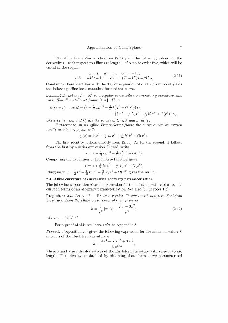
At a point of non-vanishing Euclidean curvature there is a unique conic, calledthe osculating conic, having fourth order contact with the curve at that point (or,in other words, having five coinciding points of intersection with the curve). Theaffine curvature of this conic is equal to the affine curvature of the curve at thepoint of contact. Moreover, the contact is of order five if the affine curvature hasvanishing derivative at the point of contact. In that case the point of contact is asextactic point. Again, see [3] for further details. At non-sextactic points the curveand its osculating conic cross (see also Figure 1):
Corollary 2.6. At a non-sextactic point a curve crosses its osculating conic fromright to left if its affine curvature is locally increasing at that point, and from leftto right if the affine curvature is locally decreasing.
Approximation by Conic Splines 9
Figure 1. The curve and its osculating conic (dashed). The affinecurvature is increasing in the left picture, and decreasing in theright picture.
2.6. The five-point conic
To derive error bounds for an optimal approximating conic we use the propertythat the approximating conic depends smoothly on the points of intersection withthe curve. More precisely, let α : I → R
2 be a regular curve without sextacticpoints, and let si, 1 6 i 6 5, be points on I, not necessarily distinct. The uniqueconic passing through the points α(si) is denoted by Cs, with s = (s1, s2, s3, s4, s5).If one or more of the points coincide, the conic has contact with the curve of ordercorresponding to the multiplicity of the point. For instance, if s1 = s2 6= si, i > 3,then Cs has first order contact with (is tangent to) the curve at α(s1).
If si 6= sj , for i 6= j, then the implicit quadratic equation of this conic canbe obtained as follows. Let the Veronese mapping Ψ : R
2 → R6 be defined by
Ψ(x) = (x21, x1x2, x
22, x1, x2, 1), x = (x1, x2), then the equation of the conic Cs is
f(x, s) = 0, with
f(x, s) = det(Ψ(x),Ψ(α(s1)),Ψ(α(s2)),Ψ(α(s3)),Ψ(α(s4)),Ψ(α(s5))
). (2.13)
However, if si = sj for i 6= j, then f(x, s) = 0. We obtain a quadratic equation ofthe conic Cs by (formally) dividing f(x, s) by si − sj . More precisely:
Lemma 2.7. If α is a Cm-curve, m > 4, then the conic Cs has a quadratic equationwith coefficients that are Cm−4-functions of s = (s1, s2, s3, s4, s5) ∈ R
5.
Proof. Put ψ(s) = Ψ(α(s)). The Newton development of ψ in terms of the divideddifferences of ψ up to order four associated with the points s1, . . . , s5 is given by
ψ(sk) = ψ(s1)+∑k
i=2
∏i−1j=1(sk−sj) [s1, . . . , sk]ψ, for 2 6 k 6 5. See Appendix B.
Plugging these identities into (2.13), we see that f(x, s) =∏
16j<k65
(sk−sj)F (x, s),
with
F (x, s) = det(Ψ(x), ψ(s1), [s1, s2]ψ, . . . , [s1, . . . , s5]ψ).
Since ψ is Cm, with m > 4, it follows from Appendix B that F is a Cm−4-function,with x 7→ F (x, s) being a non-vanishing quadratic function. �
In particular, if σ = (σ, . . . , σ) ∈ R5, then it follows from Appendix B,
Lemma B.1, that
F (x, σ) =1
2!3!4!det(Ψ(x), ψ(σ), ψ′(σ), ψ′′(σ), ψ′′′(σ), ψ(4)(σ)
).
10 S. Ghosh, S. Petitjean and G. Vegter
Since α contains no sextactic points, the equation F (x, σ) = 0 defines a non-degenerate conic, the osculating conic at α(σ).
If σ, % and u are three distinct points of I, then there is a unique conic Cσ,%,u
which is tangent to α at α(σ) and α(%), and passes through the point α(u). Theequation of this conic is
det(Ψ(x), ψ(σ), ψ′(σ), ψ(%), ψ′(%), ψ(u)
)= 0.
As in the proof of Lemma 2.7 one proves that Cσ,%,u is a Cm−4-function of (σ, %, u),and that it tends to the osculating conic at α(σ) as u→ σ and %→ σ.
3. Optimal conic approximation of affine spiral arcs
In this section we prove both the equioscillation property and the monotonicityproperty of the Hausdorff distance. Both properties are global, since the affinespiral is not necessarily short.
3.1. Intersections of conics and affine spirals
We start with a useful global property of affine spirals.
Proposition 3.1. 1. A conic intersects an affine spiral in at most five points,counted with multiplicity.
2. The osculating conics of an affine spiral are disjoint, and do not intersect thespiral arc except at their point of contact.
A proof of this theorem is given in [23, chapter 4]. The second part is anexercise in [3, chapter 1]. A modern proof is given in [27].
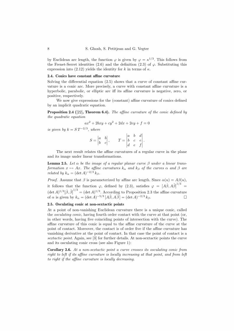
Now consider an affine spiral arc α : [u0, u1] → R2. Let Cu, u0 6 u 6 u1,
be the unique conic that is tangent to α at its endpoints, and intersects it at thepoint α(u). For u = u0 and u = u1 the conic has a triple intersection with thecurve, or, in other words, it has contact of second order with α there.
Proposition 3.2. 1. Two conics Cu and Cu′ , u 6= u′, are tangent at α(u0) andα(u1), and have no other intersections.
2. Conic Cu intersects arc α at α(u0), α(u), and α(u1), but at no other point.
Proof. 1. By Bezout’s theorem, two conics intersect in at most four points, countedwith multiplicity. Since conics Cu and Cu′ intersect with multiplicity two at eachof the points α(u0) and α(u1), there are no other intersections.
2. This is a straightforward consequence of Proposition 3.1, part 1.
�
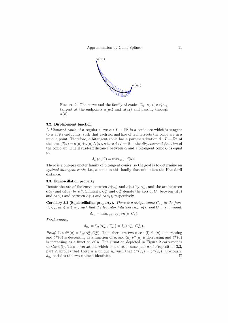
Approximation by Conic Splines 11
α(u0)
α(u1)
Figure 2. The curve and the family of conics Cu, u0 6 u 6 u1,tangent at the endpoints α(u0) and α(u1) and passing throughα(u).
3.2. Displacement function
A bitangent conic of a regular curve α : I → R2 is a conic arc which is tangent
to α at its endpoints, such that each normal line of α intersects the conic arc in aunique point. Therefore, a bitangent conic has a parameterization β : I → R
2 ofthe form β(u) = α(u)+d(u)N(u), where d : I → R is the displacement function ofthe conic arc. The Hausdorff distance between α and a bitangent conic C is equalto
δH(α,C) = maxu∈I |d(u)|.There is a one-parameter family of bitangent conics, so the goal is to determine anoptimal bitangent conic, i.e., a conic in this family that minimizes the Hausdorffdistance.
3.3. Equioscillation property
Denote the arc of the curve between α(u0) and α(u) by α−u , and the arc between
α(u) and α(u1) by α+u . Similarly, C−
u and C+u denote the arcs of Cu between α(u)
and α(u0) and between α(u) and α(u1), respectively.
Corollary 3.3 (Equioscillation property). There is a unique conic Cu∗in the fam-
ily Cu, u0 6 u 6 u1, such that the Hausdorff distance du∗of α and Cu∗
is minimal:
du∗= minu06u6u1
δH(α,Cu).
Furthermore,
du∗= δH(α−
u∗, C−
u∗) = δH(α+
u∗, C+
u∗).
Proof. Let δ±(u) = δH(α±u , C
±u ). Then there are two cases: (i) δ−(u) is increasing
and δ+(u) is decreasing as a function of u, and (ii) δ−(u) is decreasing and δ+(u)is increasing as a function of u. The situation depicted in Figure 2 correspondsto Case (i). This observation, which is a direct consequence of Proposition 3.2,part 2, implies that there is a unique u∗ such that δ−(u∗) = δ+(u∗). Obviously,du∗
satisfies the two claimed identities. �
12 S. Ghosh, S. Petitjean and G. Vegter
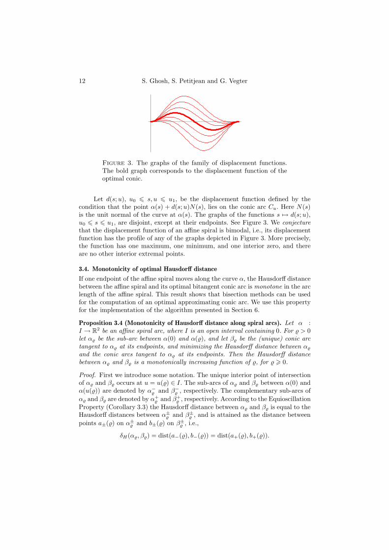
Figure 3. The graphs of the family of displacement functions.The bold graph corresponds to the displacement function of theoptimal conic.
Let d(s;u), u0 6 s, u 6 u1, be the displacement function defined by thecondition that the point α(s) + d(s;u)N(s), lies on the conic arc Cu. Here N(s)is the unit normal of the curve at α(s). The graphs of the functions s 7→ d(s;u),u0 6 s 6 u1, are disjoint, except at their endpoints. See Figure 3. We conjecturethat the displacement function of an affine spiral is bimodal, i.e., its displacementfunction has the profile of any of the graphs depicted in Figure 3. More precisely,the function has one maximum, one minimum, and one interior zero, and thereare no other interior extremal points.
3.4. Monotonicity of optimal Hausdorff distance
If one endpoint of the affine spiral moves along the curve α, the Hausdorff distancebetween the affine spiral and its optimal bitangent conic arc is monotone in the arclength of the affine spiral. This result shows that bisection methods can be usedfor the computation of an optimal approximating conic arc. We use this propertyfor the implementation of the algorithm presented in Section 6.
Proposition 3.4 (Monotonicity of Hausdorff distance along spiral arcs). Let α :I → R
2 be an affine spiral arc, where I is an open interval containing 0. For % > 0let α% be the sub-arc between α(0) and α(%), and let β% be the (unique) conic arctangent to α% at its endpoints, and minimizing the Hausdorff distance between α%
and the conic arcs tangent to α% at its endpoints. Then the Hausdorff distancebetween α% and β% is a monotonically increasing function of %, for % > 0.
Proof. First we introduce some notation. The unique interior point of intersectionof α% and β% occurs at u = u(%) ∈ I. The sub-arcs of α% and β% between α(0) andα(u(%)) are denoted by α−
% and β−% , respectively. The complementary sub-arcs of
α% and β% are denoted by α+% and β+
% , respectively. According to the EquioscillationProperty (Corollary 3.3) the Hausdorff distance between α% and β% is equal to theHausdorff distances between α±
% and β±% , and is attained as the distance between
points a±(%) on α±% and b±(%) on β±
% , i.e.,
δH(α%, β%) = dist(a−(%), b−(%)) = dist(a+(%), b+(%)).
Approximation by Conic Splines 13
The complete conic containing β% will be denoted by K%. We will repeatedly usethe following consequence of Bezout’s theorem:
Intersection Property: For 0 < %1 < %2, the conics K%1and K%2
have at most twopoints of intersection (possibly counted with multiplicity) different from α(0).
Let %1, %2 ∈ I, with 0 < %1 < %2. The regions bounded by α±%2
and β±%2
are denoted
by R±. Since K%1is either compact or unbounded, and not disjoint from the
boundary of R+, it intersects this boundary in an even number of points (countedwith multiplicity). Our strategy is to prove that β−
%1lies inside R−, or that β+
%1lies
inside R+. In the former case, we see that
δH(α%1, β%1
) = dist(a−(%1), b−(%1)) < dist(a−(%2), b−(%2)) = δH(α%2, β%2
),
whereas in the latter case
δH(α%1, β%1
) = dist(a+(%1), b+(%1)) < dist(a+(%2), b+(%2)) = δH(α%2, β%2
).
We distinguish two cases, depending on the order of u(%1) and u(%2).
Case 1: u(%1) > u(%2). Note that the conic K%1is tangent to α at α(%1), a point
contained in α%2. Therefore, in this case K%1
intersects α+%2
in an odd number ofpoints, namely, once at the point α(u(%1)) and twice at the point of tangencyα(%1).
β+%2
, the other part of boundary of R+, in an odd number of points. By theIntersection Property, this odd number is equal to one. Since both endpoints ofβ%1
lie on the same side of β%2, this point of intersection does not lie on β%1
. Inother words, the interior of β+
%1lies inside the region R+.
Case 2: u(%1) < u(%2). In this case K%1does not cross α+
%2, since it intersects α+
%2
in two coinciding points at the tangency α(%1), but at no other point. Therefore,K%1
intersects β+%2
, the other part of the boundary of R+, in at least two points (atleast one entrance and at least one exit point). By the Intersection Property, apartfrom α(0), these are the only points in which K%1
and K%2intersect. Therefore,
β−%1
intersects neither β−%2
nor α−%2
in an interior point. In other words, the interior
of β−%1
lies inside the region R−. �
Remark. A similar monotonicity property holds for the Hausdorff distance betweenan affine spiral and a bitangent parabolic arc. The proof is omitted, since it isstraightforward, and along the same lines as the proof of Proposition 3.4.
4. Affine curvature of offset curves
The main result of this section is a relation between the affine curvatures of acurve and a bitangent offset curve.
Let α : I → R2 be a regular curve parameterized by affine arc length, with
affine arc length parameter u ∈ I. Here I is an open interval, containing 0. Weconsider offset curves tangent to α at α(0) and α(%). The affine curvature of sucha curve is related to the affine curvature k of α, as indicated in the first part of the
14 S. Ghosh, S. Petitjean and G. Vegter
following Lemma. In the second part, an analogous result relates these curvatureswhen there is an additional point of intersection at α(σ).
Lemma 4.1 (Affine curvature of offset curves). Let α be a Cm-regular curve.
1. Let β : I×I → R2 be a Cn-function, such that, β(·, %) is a curve tangent to
α at α(0) and α(%), for % ∈ I. If m,n > 5, there are Cl-functions P,Q : I×I → R,with l = min(m− 5, n− 4), such that
β(u, %) = α(u) + d(u, %)(P (u, %)t(u) +Q(u, %)n(u)
), (4.1)
where d(u, %) = u2 (u−%)2. Here t(u) and n(u) are the affine tangent and the affinenormal of α, respectively. Furthermore, the affine curvature kβ(u, %) of β(·, %) at0 6 u 6 % is given by
kβ(u, %) = k(0) + 8Q(0, 0) +O(%). (4.2)
2. Let β : I × I × I → R2 be a Cn-function, such that, β(·, σ, %) is a curve tangent
to α at α(0) and α(%) and intersecting α at α(σ), for σ, % ∈ I and 0 6 σ 6 %. Ifm,n > 6, and, moreover, β also intersects α at α(σ), with 0 6 σ 6 %, then thereare Cl-functions P,Q : I × I → R, with l = min(m− 6, n− 5), such that
β(u, σ, %) = α(u) + d(u, σ, %)(P (u, σ, %)t(u) +Q(u, σ, %)n(u)
), (4.3)
where d(u, σ, %) = u2 (u−%)2 (u−σ). Furthermore, the affine curvature kβ(u, σ, %)of β(·, σ, %) at 0 6 u 6 % is given by
kβ(u, σ, %) = k(0) + k′(0)u+ 8 (5u− σ − 2%)Q(0, 0, 0) +O(%2).
Proof. 1. If α is Cm, then the functions (u, %) 7→ [β(u, %) − α(u), n(u)] and(u, %) 7→ [β(u, %) − α(u), t(u)] are of class Cmin(m−1,n). For fixed %, these func-tions have double zeros at u = 0 and u = %. The Division Property, cf. Appen-dix B, Lemma B.2, guarantees the existence of Cmin(m−5,n−4)-functions P andQ satisfying [β(u, %) − α(u), n(u)] = d(u, %)P (u, %) and [β(u, %) − α(u), t(u)] =d(u, %)Q(u, %). In other words, P and Q satisfy identity (4.1).
According to Proposition 2.3 the affine curvature of the curve β(·, %) is aCn−4-function given by
kβ =1
ϕ5[βuu, βuuu] +
1
ϕ4(ϕuu ϕ− 3ϕ2
u), (4.4)
ϕ = [βu, βuu]1/3
. In (4.4), the functions kβ , ϕ, β, and their partial derivativesare evaluated at (u, %). Since n > 5, and 0 6 u 6 %, it follows that kβ(u, %) =kβ(u, 0) + O(%). So, to prove (4.2), it is sufficient to determine β(u, 0) and itsderivatives up to order four. Writing β0(u) = β(u, 0), we see that
β0(u) = α(u) + f(u) (P0 t(u) +Q0 n(u)) +O(u5),
Approximation by Conic Splines 15
where f(u) = u4, P0 = P (0, 0) andQ0 = Q(0, 0). In view of the affine Frenet-Serretidentities (2.7) we get
β′0 = (1 + f ′ P0) t+ f ′Q0 n+O(u4),
β′′0 = f ′′ P0 t+ (1 + f ′′Q0)n+O(u3), (4.5)
β′′′0 = (−k + f ′′′ P0) t+ f ′′′Q0 n+O(u2).
Here the functions β0, f , t, n and k, as well as their derivatives, are evaluated at
u. Since ϕ(u, 0) = [β′0(u), β
′′0 (u)]
13 , we use the first two identities of (4.5) to derive
ϕ(u, 0) = 1 + 13 f
′′(u)Q0 +O(u3) = 1 + 4 u2Q0 +O(u3).
Similarly, using the second and third identity of (4.5) we get
[β′′0 (u), β′′′
0 (u)] = k(u) +O(u) = k(0) + 8Q0 +O(u).
Identity (4.2) is obtained by plugging these expressions into (4.4).
2. Now we turn to the case where the offset curve not only is tangent toα at its endpoints, but also has an additional point of intersection at α(σ). Theexistence of functions P and Q satisfying (4.3) is proven as in Part 1, using theDivision Property. Again the affine curvature of β is given by (4.4), where thistime the functions kβ , ϕ, β, and their partial derivatives are evaluated at (u, σ, %).
In (4.3) we have d(u, σ, %) = u5 − (2%+ σ)u4 + O(%2 + σ2), P = P0 + O(u),and Q = Q0 +O(u). Focusing on the essential terms only, we rewrite (4.3) as:
β = α+ (u5 − (2%+ σ)u4) (P0 t+Q0 n) +O(u6) +O((% + σ)u5) +O(%2 + σ2).(4.6)
Here α, t and n are evaluated at u, and β at (u, σ, %). For a smoother presentation,we introduce the following terminology. The class Oi(u, σ, %), 0 6 i 6 4, consistsof all Cm−i-functions of the form O(u6−i) + O((% + σ)u5−i) + O(%2 + σ2). Usingthis notation we rewrite (4.6) as
β = α+ f (P0 t+Q0 n) +O0(u, σ, %).
where f(u, σ, %) = u5 − (2%+ σ)u4.
If g ∈ Oi(u, σ, %), then gu ∈ Oi+1(u, σ, %), for 1 6 i 6 4. Therefore, we get, asin (4.5):
βu = (1 + fu P0) t+ fuQ0 n+O1(u, σ, %),
βuu = fuu P0 t+ (1 + fuuQ0)n+O2(u, σ, %), (4.7)
βuuu = (−k + fuuu P0) t+ fuuuQ0 n+O3(u, σ, %).
Since ϕ = [βu, βuu]13 , we use the first two identities of (4.7) to derive
ϕ = 1 + 13 fuuQ0 +O2(u, σ, %),
16 S. Ghosh, S. Petitjean and G. Vegter
so ϕ = 1 + O3(u, σ, %), ϕ2u = O4(u, σ, %), and ϕuu = 1
3 Q0 fuuuu + O4(u, σ, %).Similarly, using the second and third identity of (4.5) we get
[βuu, βuuu] = k(u) +O4(u, σ, %).
It follows that
kβ(u, σ, %) = k(u) + 13 fuuuu Q0 +O4(u, σ, %)
= k(0) + k′(0)u+ 8 (5u− σ − 2%)Q0 +O(%2).
Note that in the last identity we used that O4(u, σ, %) = O(u2 +σ2 + %2) = O(%2),since 0 6 u, σ 6 %. This concludes the proof of the second part. �
If the offset curves are bitangent conics, the affine curvature of these conicscan be expressed in the Euclidean and affine curvature of the curve α at the pointsof intersection. Furthermore, we can determine the displacement function up toterms of order five if the conic is a parabola, and up to terms of order six in thegeneral case. These results will enable us to determine an asymptotic expressionfor the Hausdorff distance between a small arc and its optimal bitangent conic.
Corollary 4.2 (Bitangent conics). Let α be a strictly convex regular Cm-curve.
1. If m > 8, a parabolic arc tangent to α at α(0) and α(%) has the form
β(u, %) = α(u) + u2 (%− u)2D(u, %)N(u), (4.8)
where D is a Cm−8-function with D(0, 0) = − 18 k(0)κ(0)1/3. Here N(u) is the
Euclidean normal of α, and κ is its Euclidean curvature.
2. If m > 9, a conic arc tangent to α at α(0) and α(%) and intersecting at α(σ),with 0 6 σ 6 %, has the form
β(u, σ, %) = α(u) + u2 (%− u)2 (u− σ)D(u, σ, %)N(u), (4.9)
where D is a Cm−9-function with D(0, 0, 0) = − 140 k
′(0)κ(0)1/3. Moreover, itsaffine curvature is of the form
kβ(σ, %) = 15 (2k(0) + k(σ) + 2k(%)) +O(%2).
Proof. 1. Obviously, the family of parabolic arcs can be written in the formβ(u, %) = α(u) + d(u, %)N(u), provided % is sufficiently small. According toLemma 2.7, β is a Cm−4-function, so d = [T, β − α] is a Cm−4-function withdouble zeros at u = 0 and u = %. According to Lemma 4.1, the parabola has aparameterization of the form (4.1), where P and Q are Cm−8-functions. Therefore,d(u, %) = u2 (u−%)2Q(u, %) [T (u), n(u)], so β is of the form (4.8) with D = Q [T, n].In particular, D is a Cm−8-function. Comparing this expression with identity (4.1)in Lemma 4.1, we see that D(u, %) = Q(u, %) [T (u), n(u)]. From (2.9) we concludethat D(0, 0) = κ(0)1/3Q(0, 0). Since the affine curvature of a parabolic arc is iden-tically zero, Part 1 of Lemma 4.1 yields Q(0, 0) = − 1
8 k(0), yielding the value forD(0, 0) stated in Part 1.
Approximation by Conic Splines 17
2. As in Part 1 we prove that β has a parameterization of the form (4.9), where Dis a Cm−9-function. The affine curvature of a conic arc is constant, so Part 2of Lemma 4.1 yields Q(0, 0, 0) = − 1
40 k′(0). Since also in this case we have
D(0, 0, 0) = κ(0)1/3Q(0, 0, 0), we conclude that D(0, 0, 0) has the value statedin Part 2. Furthermore, (4.2) yields
kβ = k(0) + 15 (σ + 2%) k′(0) +O(%2) = 1
5 (2k(0) + k(σ) + 2k(%)) +O(%2).
This concludes the proof of the second part. �
Remarks. 1. The second part of Corollary 4.2 can be generalized in the sense thatthe affine curvature of a conic intersecting a strictly convex arc at five points isequal to the average of the affine curvatures of the curve at these five points, upto quadratic terms in the affine length of the arc. The proof is similar to the onegiven above.
2. We conjecture that the ‘loss of differentiability’ is less than stated in Corol-lary 4.2. More precisely, we expect thatD is of class Cm−4 for a bitangent parabolicarc, and of class Cm−5 for a bitangent conic arc.
5. Complexity of conic splines
In this section our goal is to determine the Hausdorff distance of a conic arc ofbest approximation to an arc of α of Euclidean length σ > 0, that is tangent toα at its endpoints. If the conic is a parabola, these conditions uniquely determinethe parabolic arc. If we approximate with a general conic, there is one degree offreedom left, which we use to minimize the Hausdorff distance between the the arcof α and the approximating conic arc β. As we have seen in Section 3, the optimalconic arc intersects the arc of α in an interior point.
The main result of this section gives an asymptotic bound on this Hausdorffdistance.
Theorem 5.1 (Error in parabolic and conic spline approximation). Let β be aconic arc tangent at its endpoints to an arc of a regular curve α of length σ, withnon-vanishing Euclidean curvature.
1. If α is a C8-curve, and β is a parabolic arc, then the Hausdorff distance betweenthese arcs has asymptotic expansion
δH(α, β) = 1128 |k0|κ5/3
0 σ4 +O(σ5), (5.1)
where κ0 and k0 are the Euclidean and affine curvatures of α at one of its end-points, respectively.
2. If α is a C9-curve, and β is a conic arc, then the Hausdorff distance betweenthese arcs is minimized if the affine curvature of β is equal to the average of the
18 S. Ghosh, S. Petitjean and G. Vegter
affine curvatures of α at its endpoints, up to quadratic terms in the length of α.In this case this Hausdorff distance has asymptotic expansion
δH(α, β) = 12000
√5|k′0|κ2
0 σ5 +O(σ6), (5.2)
where κ0 is the Euclidean curvature of α at one of its endpoints, and k′0 is thederivative of the affine curvature of α at one of its endpoints.
Proof. 1. According to Corollary 4.2, the parabolic arc has a parameterization ofthe form (4.8). It follows from Appendix C, Lemma C.1, applied to the displace-ment function d(u) = u2 (%− u)2D(u, %), cf. (4.8), that
δH(α, β) = 116 |D(0, 0)| %4 +O(%5). (5.3)
From Lemma 2.1, part 1, we derive
% = κ1/30 σ +O(σ2). (5.4)
Since D(0, 0) = − 18 k(0)κ(0)1/3, we conclude from (5.3) and (5.4) that the Haus-
dorff distance satisfies (5.1).
2. Again, according to Corollary 4.2, cf. (4.9), a best approximating conic arc has aparameterization of the form (4.9), with D(0, 0, 0) = − 1
40 k′(0)κ(0)1/3. Applying
Appendix C, Lemma C.1 to the displacement function d(u) = u2 (u − σ) (% −u)2D(u, σ, %), cf. (4.9), we see that
δH(α, β) = 150
√5|D(0, 0, 0)| %5 +O(%6), (5.5)
where the optimal conic intersects the curve α for σ = σ(%) = 12 %+O(%2). Identities
(5.4) and (5.5) imply that the Hausdorff distance is given by (5.2). Finally, theaffine curvature of this conic is
15 (2k(0) + k(1
2 %+O(%2)) + 2k(%)) +O(%2) = 12 (k(0) + k(%)) +O(%2).
This concludes the proof of the main theorem of this section. �
Remark. It would be interesting to give a direct geometric proof of the fact thatthe best approximating conic has affine curvature equal to the average of the affinecurvatures of α at its endpoints.
The preceding result gives an asymptotic expression for the minimal num-ber of elements of an optimal parabolic or conic spline in terms of the maximalHausdorff distance.
Corollary 5.2 (Complexity of parabolic and conic splines). Let α : [0, L] → R2 be
a regular curve with non-vanishing Euclidean curvature of length L, parameterizedby Euclidean arc length, and let κ(s) and k(s) be its Euclidean and affine curvatureat α(s), respectively.
Approximation by Conic Splines 19
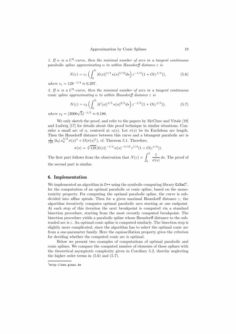
1. If α is a C8-curve, then the minimal number of arcs in a tangent continuousparabolic spline approximating α to within Hausdorff distance ε is
N(ε) = c1
(∫ L
0
|k(s)|1/4 κ(s)5/12ds)
ε−1/4(1 +O(ε1/4)), (5.6)
where c1 = 128−1/4 ≈ 0.297.
2. If α is a C9-curve, then the minimal number of arcs in a tangent continuousconic spline approximating α to within Hausdorff distance ε is
N(ε) = c2
(∫ L
0
|k′(s)|1/5 κ(s)2/5ds)
ε−1/5(1 +O(ε1/5)), (5.7)
where c2 = (2000√
5)−1/5 ≈ 0.186.
We only sketch the proof, and refer to the papers by McClure and Vitale [19]and Ludwig [17] for details about this proof technique in similar situations. Con-sider a small arc of α, centered at α(s). Let σ(s) be its Euclidean arc length.Then the Hausdorff distance between this curve and a bitangent parabolic arc is1
128 |k0|κ5/30 σ(s)4 +O(σ(s)5), cf. Theorem 5.1. Therefore,
σ(s) =4√
128 |k(s)|−1/4 κ(s)−5/12 ε1/4(1 +O(ε1/4)).
The first part follows from the observation that N(ε) =
∫ L
0
1
σ(s)ds. The proof of
the second part is similar.
6. Implementation
We implemented an algorithm in C++ using the symbolic computing library GiNaC1,
for the computation of an optimal parabolic or conic spline, based on the mono-tonicity property. For computing the optimal parabolic spline, the curve is sub-divided into affine spirals. Then for a given maximal Hausdorff distance ε, thealgorithm iteratively computes optimal parabolic arcs starting at one endpoint.At each step of this iteration the next breakpoint is computed via a standardbisection procedure, starting from the most recently computed breakpoint. Thebisection procedure yields a parabolic spline whose Hausdorff distance to the sub-tended arc is ε. An optimal conic spline is computed similarly. The bisection step isslightly more complicated, since the algorithm has to select the optimal conic arcfrom a one-parameter family. Here the equioscillation property gives the criterionfor deciding whether the computed conic arc is optimal.
Below we present two examples of computations of optimal parabolic andconic splines. We compare the computed number of elements of these splines withthe theoretical asymptotic complexity given in Corollary 5.2, thereby neglectingthe higher order terms in (5.6) and (5.7).
1http://www.ginac.de
20 S. Ghosh, S. Petitjean and G. Vegter
−1
31 4
−2
−2−3
0
−4
620 5
1
−3
−1 5420−2
1
−4
−3
3 6
−2
−1
1−1−3
0
−4
0
−1
32
−2
1
−3
−3 6−1 1 54
0
−2 20 1−1−2
1
6
−3
3−3 4
−1
−4
−2
5
0
−1
4
0
6
−2
−4
−3
1
−1−3 20−2 3 51 5
−4
4
0
−1
−1
1
−3
2−3
−2
1 60−2 3 6
−3
32
−2
−2 1−3
1
−1 5
−1
−4
0
40 0−2
1
6−1 2
−1
4 5
−4
−3
0
−2
3
−3
1
(a) Conic spline approximation
2
0
−2
−4
2 5
1
−1
−3
−5
640 1−2 3−1−3 2−1−3 −2 6
−2
1
1
−1
3
0
−3
−4
40 5
1
40 51 6−2 −1−3
−2
−1
0
2
−3
−4
3 4
−3
−4
−2
1
−3 −2 6−1 2
0
−1
5310
−3
−4
−1
1
2
−3
4
0
61 3−1 0
−2
5−2
−1
−2 4
−3
−2
−3 −1 0 6
0
1 5
−4
1
32
1
−1
62−3
−3
1 430
−4
−1
−2
0
5−2
(b) Parabolic spline approximation
Figure 4. Approximation of the spiral for ε ranging between10−1 to 10−8.
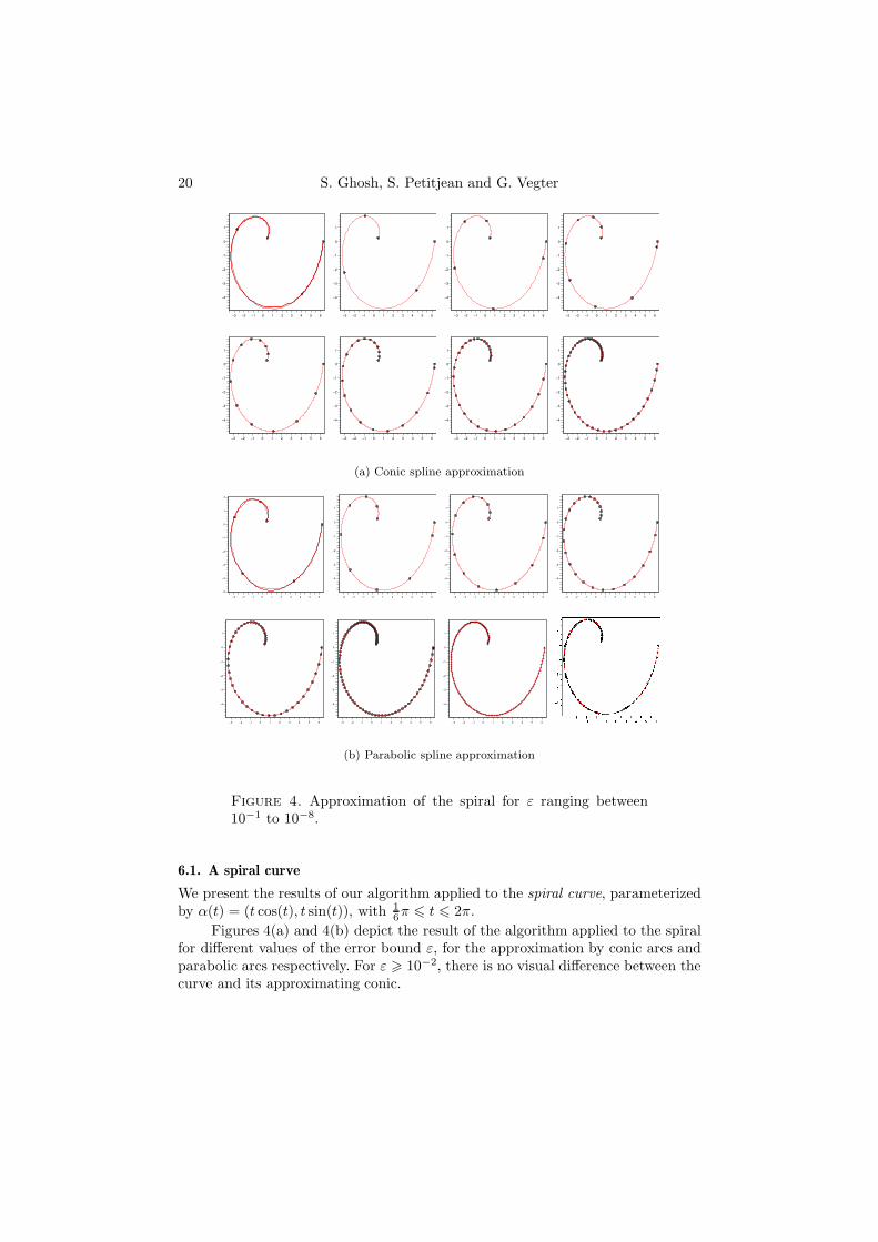
6.1. A spiral curve
We present the results of our algorithm applied to the spiral curve, parameterizedby α(t) = (t cos(t), t sin(t)), with 1
6π 6 t 6 2π.
Figures 4(a) and 4(b) depict the result of the algorithm applied to the spiralfor different values of the error bound ε, for the approximation by conic arcs andparabolic arcs respectively. For ε > 10−2, there is no visual difference between thecurve and its approximating conic.
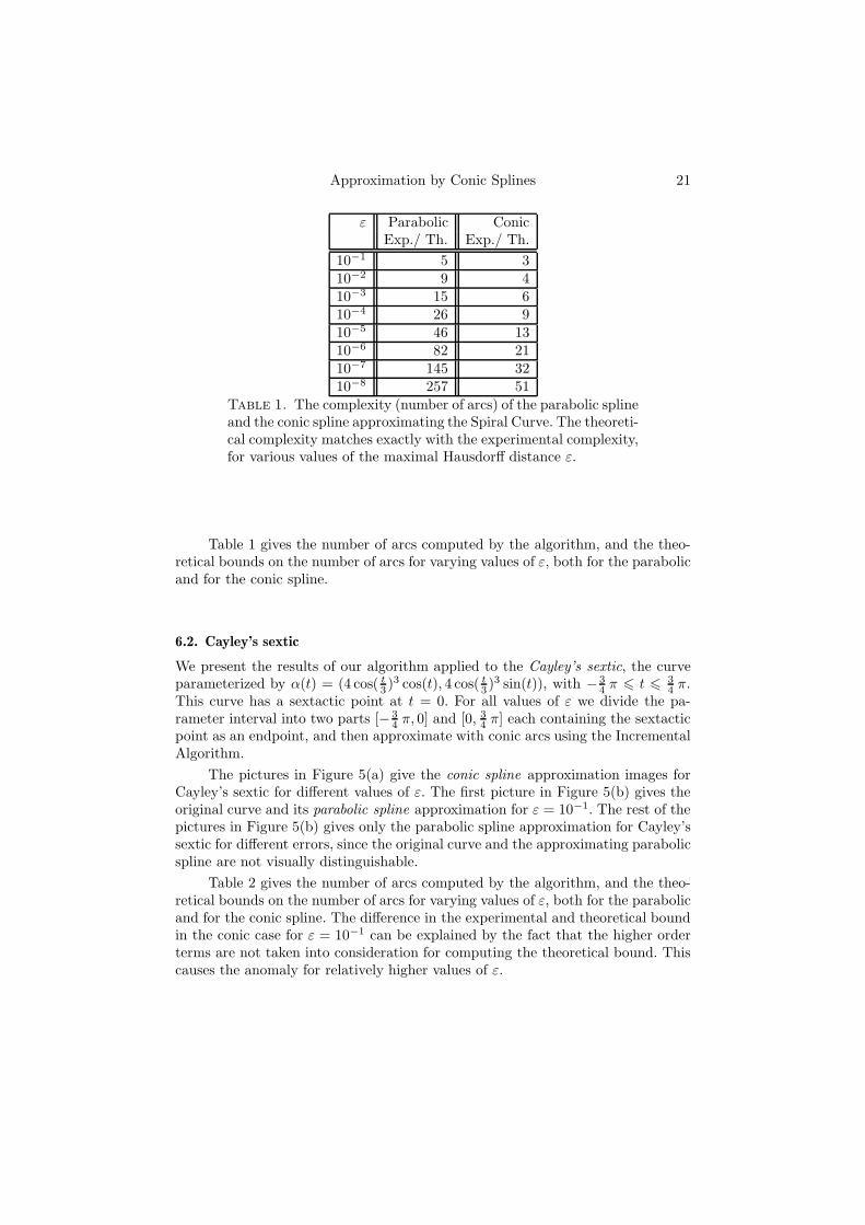
Approximation by Conic Splines 21
ε Parabolic ConicExp./ Th. Exp./ Th.
10−1 5 310−2 9 410−3 15 610−4 26 910−5 46 1310−6 82 2110−7 145 3210−8 257 51
Table 1. The complexity (number of arcs) of the parabolic splineand the conic spline approximating the Spiral Curve. The theoreti-cal complexity matches exactly with the experimental complexity,for various values of the maximal Hausdorff distance ε.
Table 1 gives the number of arcs computed by the algorithm, and the theo-retical bounds on the number of arcs for varying values of ε, both for the parabolicand for the conic spline.
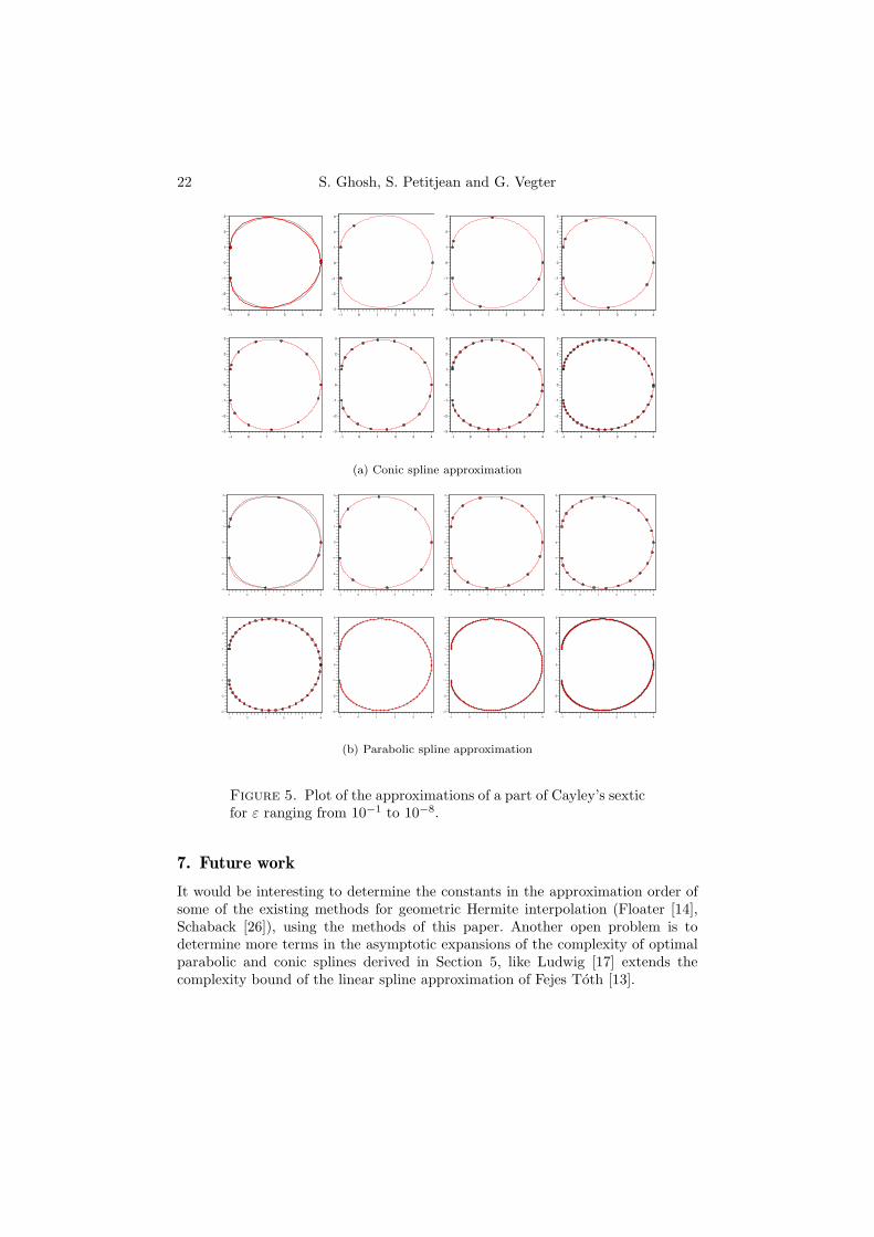
6.2. Cayley’s sextic
We present the results of our algorithm applied to the Cayley’s sextic, the curveparameterized by α(t) = (4 cos( t
3 )3 cos(t), 4 cos( t3 )3 sin(t)), with − 3
4 π 6 t 6 34 π.
This curve has a sextactic point at t = 0. For all values of ε we divide the pa-rameter interval into two parts [− 3
4 π, 0] and [0, 34 π] each containing the sextactic
point as an endpoint, and then approximate with conic arcs using the IncrementalAlgorithm.
The pictures in Figure 5(a) give the conic spline approximation images forCayley’s sextic for different values of ε. The first picture in Figure 5(b) gives theoriginal curve and its parabolic spline approximation for ε = 10−1. The rest of thepictures in Figure 5(b) gives only the parabolic spline approximation for Cayley’ssextic for different errors, since the original curve and the approximating parabolicspline are not visually distinguishable.
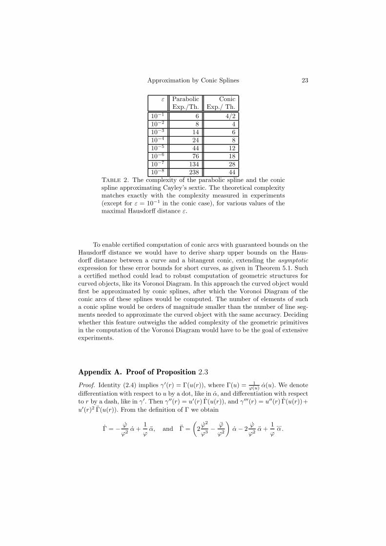
Table 2 gives the number of arcs computed by the algorithm, and the theo-retical bounds on the number of arcs for varying values of ε, both for the parabolicand for the conic spline. The difference in the experimental and theoretical boundin the conic case for ε = 10−1 can be explained by the fact that the higher orderterms are not taken into consideration for computing the theoretical bound. Thiscauses the anomaly for relatively higher values of ε.
22 S. Ghosh, S. Petitjean and G. Vegter
−1
2
−1
1
−3
0
0 41 2 3
3
−2
−1
1
−2
1
2
0
3
−1
3 420
−3
40 1
0
2
3
3
−3
−1
−1
−2
1
2
4
3
31−1
0
1
0
−3
2
−1
2
−2
−1
3 40
0
−2
1−1
2
1
3
−3
2 1
2
−2
4
−1
1
−1
−3
0
0 3
3
2 1
0
2
−3
3
1
0
−1
−2
432−1
2
3
4
−3
1
0
3−1
−2
2
1
−1
0
(a) Conic spline approximation
0
3
1
3−1
0
2
−1
−2
−3
4
2
1 4
−2
3
1
−3
0
0 2
2
−1
3−1
1
3
3
−1
42
−3
1
1
0
2
−2
−1 0 320
3
−1
−1
−2
2
1
0
4
−3
1
−1
1
−3
3
32 4
−2
1
0
0
2
−1
−1
3
−2
1
−1
2
0
1
3 42
0
−3 −3
−1
3
31
1
2
−2
2
0 4
0
−1
−2
−3
43−1
0
3
2
1
0 1
−1
2
(b) Parabolic spline approximation
Figure 5. Plot of the approximations of a part of Cayley’s sexticfor ε ranging from 10−1 to 10−8.
7. Future work
It would be interesting to determine the constants in the approximation order ofsome of the existing methods for geometric Hermite interpolation (Floater [14],Schaback [26]), using the methods of this paper. Another open problem is todetermine more terms in the asymptotic expansions of the complexity of optimalparabolic and conic splines derived in Section 5, like Ludwig [17] extends thecomplexity bound of the linear spline approximation of Fejes Toth [13].
Approximation by Conic Splines 23
ε Parabolic ConicExp./Th. Exp./ Th.
10−1 6 4/210−2 8 410−3 14 610−4 24 810−5 44 1210−6 76 1810−7 134 2810−8 238 44
Table 2. The complexity of the parabolic spline and the conicspline approximating Cayley’s sextic. The theoretical complexitymatches exactly with the complexity measured in experiments(except for ε = 10−1 in the conic case), for various values of themaximal Hausdorff distance ε.
To enable certified computation of conic arcs with guaranteed bounds on theHausdorff distance we would have to derive sharp upper bounds on the Haus-dorff distance between a curve and a bitangent conic, extending the asymptoticexpression for these error bounds for short curves, as given in Theorem 5.1. Sucha certified method could lead to robust computation of geometric structures forcurved objects, like its Voronoi Diagram. In this approach the curved object wouldfirst be approximated by conic splines, after which the Voronoi Diagram of theconic arcs of these splines would be computed. The number of elements of sucha conic spline would be orders of magnitude smaller than the number of line seg-ments needed to approximate the curved object with the same accuracy. Decidingwhether this feature outweighs the added complexity of the geometric primitivesin the computation of the Voronoi Diagram would have to be the goal of extensiveexperiments.
Appendix A. Proof of Proposition 2.3
Proof. Identity (2.4) implies γ′(r) = Γ(u(r)), where Γ(u) = 1ϕ(u) α(u). We denote
differentiation with respect to u by a dot, like in α, and differentiation with respectto r by a dash, like in γ′. Then γ′′(r) = u′(r) Γ(u(r)), and γ′′′(r) = u′′(r) Γ(u(r))+
u′(r)2 Γ(u(r)). From the definition of Γ we obtain
Γ = − ϕ
ϕ2α+
1
ϕα, and Γ =
(
2ϕ2
ϕ3− ϕ
ϕ2
)
α− 2ϕ
ϕ2α+
1
ϕ
...α.
24 S. Ghosh, S. Petitjean and G. Vegter
Furthermore, since u′(r) = 1ϕ(u(r)) , it follows that u′′(r) = − ϕ(u(r))
ϕ(u(r))3 . Therefore,
γ′′(r) = − ϕ
ϕ3α+
1
ϕ2α, and γ′′′(r) =
(
3ϕ2
ϕ5− ϕ
ϕ4
)
α− 3ϕ
ϕ4α+
1
ϕ3
...α,
where we adopt the convention that ϕ, α, and their derivatives are evaluated atu = u(r). Hence, the affine curvature of α at u ∈ I is given by
k(u) = [γ′′, γ′′′]
=1
ϕ5[α,
...α ] −
(
3ϕ2
ϕ7− ϕ
ϕ6
)
[α, α] + 3ϕ2
ϕ7[α, α] − ϕ
ϕ6[α,
...α ]
=1
ϕ5[α,
...α ] +
ϕ
ϕ6[α, α] − ϕ
ϕ6[α,
...α ].
From (2.3) it follows that [α, α] = ϕ3 and [α,...α ] = 3ϕ2 ϕ. Using the latter
identity we obtain expression (2.12) for the affine curvature of α. �
Appendix B. Divided differences and the Division Property
Recall that, for a real-valued function f defined on an interval I and pointsx0, x1, . . . , xn ∈ I, the n-th divided difference [x0, . . . , xn]f is defined as the coeffi-cient of xn in the polynomial of degree n that interpolates f at x0, x1, . . . , xn. Thisdefinition is equivalent to the well-known recursive definition; see [7, Chapter 4]or [25, Chapter 5]. The interpolating polynomial can be written in the Newtonform
p(x) = f(x0) + (x− x0) [x0, x1]f + · · · + (x− x0) · · · (x− xn−1) [x0, . . . , xn]f.(B.1)
The n-th divided difference is well defined if the points are distinct. However, if fis sufficiently differentiable on I, then the n-th divided difference is also defined ifsome of the points coincide. More precisely, if f is a Cn-function, then the n-thdivided difference has the following integral representation, known as the Hermite-Genocchi identity:
[x0, x1, · · · , xn] f =
∫
Σn
f (n)(t0x0 + t1x1 + · · · + tnxn) dt1 · · · dtn,
where t0 = 1 − ∑ni=1 ti, and the domain of integration is the standard Σn =
{(t1, . . . , tn) | t1 + · · · + tn 6 1, ti > 0, for i = 0, 1, . . . , n}. For a proofwe refer to [4, Chapter 1], [20] or [21]. The Hermite-Genocchi identity impliesthat [x0, x1, · · · , xn] f is symmetric and continuous in (x0, x1, . . . , xn). If f isa Cm-function, with m > n, this divided difference is a Cm−n-function of(x0, x1, . . . , xn). Furthermore, if xi = ξ for i = 0, . . . , n, then
[ξ, . . . , ξ︸ ︷︷ ︸
n+1
] f =1
n!f (n)(ξ). (B.2)
Approximation by Conic Splines 25
Furthermore, taking x0 = · · · = xn−1 = ξ, and xn = x, we see that
[ξ, . . . , ξ︸ ︷︷ ︸
n
, x] f =1
(n− 1)!
∫ 1
u=0
(1 − u)n−1f (n)((1 − u)ξ + ux
)du. (B.3)
The key result used in this paper is the following ‘Newton development’ of afunction f , akin to the Taylor series expansion.
Lemma B.1. Let f : I → R be a Cm-function defined on an interval I ⊂ R, andlet x0, . . . , xn−1 ∈ I. Then
f(x) = f(x0) +
n−1∑
k=1
k−1∏
i=0
(x− xi) [x0, . . . , xk] f +
n−1∏
i=0
(x− xi) [x0, x1, · · · , xn−1, x] f.
If m > n, then [x0, x1, · · · , xn−1, x] f is a Cn−m-function of x. Furthermore, ifx0 = . . . = xn−1 = ξ, then the preceding identity reduces to the Taylor expansionwith integral remainder:
f(x) = f(ξ)+∑n−1
k=1(x−ξ)k
k! f (k)(ξ)+ (x−ξ)n
(n−1)!
∫ 1
u=0(1−u)n−1 f (n)(ux+(1−u)ξ) du.
The result follows from the observation that the polynomial p, definedby (B.1), interpolates f at x0, . . . , xn, so in particular f(xn) = p(xn). Takingxn = x yields the first identity. The Taylor expansion follows using identities (B.2)and (B.3).
Since [x1, . . . , xk] f = 0 if f(xi) = 0, 1 6 i 6 k, a straightforward conse-quence of Newton’s expansion (Lemma B.1) is the following.
Lemma B.2 (Division Property). Let I ⊂ R be an interval containing pointsx1, . . . , xn, not necessarily distinct, and let f : I → R be a Cm-function, m > n,having a zero at xi, for 1 6 i 6 n. Then
f(x) =
n∏
i=1
(x− xi) [x1, . . . , xn, x] f.
where the divided difference [x1, . . . , xn, x] f is a Cm−n-function of x.
Appendix C. Approximation of n-flat functions
In this section we derive error bounds for univariate real functions with multiplezeros at the endpoints of some small interval [0, r]. To stress that the error alsodepends on the size of the interval we consider a one-parameter family of functions(u, r) 7→ f(u, r), where r is a small positive parameter. We look for a bound of theerror
max06u6r |f(u, r)|.To obtain asymptotic bounds for this error as r goes to zero, we assume that thefunction f is defined on a neighborhood of (0, 0) in R × R.
26 S. Ghosh, S. Petitjean and G. Vegter
Lemma C.1. Let I ⊂ R be an interval which is a neighborhood of 0 ∈ R.
1. Let f : I × I → R be a Cm-function such that the function u 7→ f(u, r) has ann-fold zero at u = 0 and at u = r, with 2n+ 2 6 m. Then
max06u6r |f(u, r)| =1
22n (2n)!
∣∣∣∣
∂2nf
∂u2n (0, 0)
∣∣∣∣r2n +O(r2n+1).
2. Let f : I × I × I → R be a Cm-function such that the function u 7→ f(u, s, r)has an n-fold zero at u = 0 and at u = r, and an additional single zero at u = s,with 2n+ 3 6 m. Let
δ(s, r) = max06u6r |f(u, s, r)|.Then δ is a continuous function, and
min06s6r δ(s, r) =cn
(2n+ 1)!
∣∣∣∣
∂2n+1f
∂u2n+1 (0, 0, 0)
∣∣∣∣r2n+1 +O(r2n+2), (C.1)
where
cn =nn
2n+1 (2n+ 1)n+ 1
2
.
Moreover, the minimum in (C.1) is attained at s = s0(r), where s0 is a Cm−2n+1-function, with s0(0) = 1
2 .
Proof. 1. We prove that, for r > 0 sufficiently small, the function u 7→ f(u, r)has a unique extremum in the interior of the interval (0, r). According to theDivision Property (see Appendix B, Lemma B.2), there is a Cm−2n-function F :
I × I → R such that f(u, r) = un (r − u)n F (u, r). Observe that∂2nf
∂u2n (0, 0) =
(−1)n (2n)!F (0, 0).
Note that the ‘model function’ g(u) = un (r − u)n F (0, 0) has its extremevalue 1
22nF (0, 0) on 0 6 u 6 r at u = 12r. We shall prove that the function f(u, r)
has its extreme value at u = 12r+O(r2). To this end we apply the Implicit Function
Theorem to solve the equation∂f∂u
(u, r) = 0.
Since 0 6 u 6 r, we scale the variable u by introducing the variable x suchthat u = rx, with 0 6 x 6 1, and observe that f(rx, r) = r2n f(x, r), with
f(x, r) = xn(1 − x)n F (rx, r). Therefore,
∂f
∂x(x, r) = nxn−1(1 − x)n−1E(x, r),
where E(x, r) = (1−2x)F (0, 0)+O(r), uniformly in 0 6 x 6 1. Since x 7→ ∂f∂x
(x, r)
has an (n − 1)-fold zero at x = 0 and x = r, the Division Property allows us
to conclude that E is a Cm−2n+1-function. Since E(12 , 0) = 0, and ∂E
∂x(12 , 0) =
−2F (0, 0) 6= 0, the Implicit Function Theorem tells us that there is a unique
Approximation by Conic Splines 27
Cm−2n+1-function r 7→ x(r) with x(0) = 12 and
∂f∂x
(x(r), r) = 0. Therefore, f(·, r)has a unique extremum at x = x(r). Hence,
max06u6r |f(u, r)| = |f(x(r), r)| r2n
= |f(12 , 0)| r2n +O(r2n+1)
=|F (0, 0)|
22nr2n +O(r2n+1)
=1
22n (2n)!
∣∣∣∣
∂2nf
∂u2n (0, 0)
∣∣∣∣r2n +O(r2n+1).
2. The proof of the second part goes along the same lines, but is slightly morecomplicated due to the occurrence of two critical points of the function f(·, s, r)in the interior of the interval (0, r). Again, the Division Property guarantees theexistence of a Cm−2n−1-function F : I × I × I → R such that f(u, s, r) = un (r −u)n (s− u)F (u, s, r).
The ‘model function’ g(u) = un (r − u)n (s − u)F (0, 0, 0) has two criticalpoints for 0 6 u 6 r: one on the interval [0, s] and one on the interval [s, r]. Thederivative of this function is of the form
g′(u) = un−1 (r − u)n−1(−(2n+ 1)u2 + (2ns+ n+ 1)u− ns
)F (0, 0, 0).
A straightforward calculation shows that g′ has two zeros u±(s), and that thecritical values of g at these zeros are equal iff s = 1
2 . In the remaining part of theproof we show that the function f(·, s, r) has its extreme values at u = u±(s) +O(r2), again by applying the Implicit Function Theorem to solve the equation∂f∂u
(u, s, r) = 0.
The critical values of f(·, s, r). Putting u = rx and s = ry, with 0 6 x, y 6
1, we obtain f(rx, ry, r) = r2n+1 f(x, y, r), with f(x, y, r) = xn (1 − x)n (x −y)F (rx, ry, r). To determine the critical points of x 7→ f(x, y, r) on the interval(0, 1), we observe that
∂f
∂x(x, y, r) = xn−1 (1 − x)n−1Q(x, y, r), (C.2)
where Q is a function of the form
Q(x, y, r) =(−(2n+ 1)x2 + (2ny + n+ 1)x− ny
)F (0, 0, 0) +O(r),
uniformly in x, y ∈ [0, 1]. Since ∂f∂x
is a Cm−1-function such that x 7→ ∂f∂x
(x, r) has
(n− 1)-fold zeros at x = 0 and x = 1, the Division Property allows us to concludethat Q, determined by (C.2), is a Cm−2n+1-function.
Assume F (0, 0, 0) > 0 (the case F (0, 0, 0) < 0 goes accordingly). Then, if
0 < y < 1, the function x 7→ f(x, y, 0) has one minimum at x = x0−(y) and one
maximum at x = x0+(y), where x0
± are the zeros of the quadratic function x 7→Q(x, y, 0). Since
∂Q∂x
(x0±(y), y, 0) 6= 0, the Implicit Function Theorem guarantees
28 S. Ghosh, S. Petitjean and G. Vegter
the existence of Cm−2n+1-functions x± : I × I → R, with x−(y, r) < x+(y, r),such that x±(y, 0) = x0
±(y), and Q(x±(y, r), y, r) = 0. So, in view of (C.2), the
function x 7→ f(x, y, r) has one minimum at x = x−(y, r), and one maximum atx = x+(y, r). Putting
δ(y, r) = max06x61 |f(x, y, r)|, (C.3)
we see that
δ(y, r) = max(|f(x−(y, r), y, r)|, |f (x+(y, r), y, r)|
).
The minimax norm of the family {f(·, s, r) | s ∈ [0, r]}. For fixed x and r, with
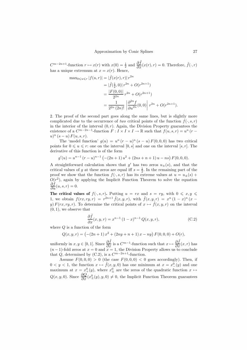
0 < x < 1 and r > 0 sufficiently small, the function y 7→ f(x, y, r) is decreasing.See Figure 6. This follows from the observation that
∂f
∂y(x, y, r) = −xn(1 − x)nE(x, y, r),
with E(x, y, r) = F (0, 0, 0) + O(r), uniformly in x, y ∈ [0, 1]. Therefore, there isa %0 > 0 such that, for 0 6 r 6 %0, we have E(x, y, r) > 0 for 0 6 x, y 6 1, and
hence∂f∂y
(x, y, r) < 0.
0.2 0.4 0.6 0.8 1
Figure 6. Graph of the function x 7→ f(x, y, r), for r fixed andy = y0 (solid), y = y1 (dashed), and y = y2 (dotted), with y0 <
y1 < y2.
From this observation it follows that, for fixed r and y ranging from 0 to 1,the graphs of the functions x 7→ f(x, y, r) are disjoint, except at their endpoints.
See again Figure 6. Therefore, the function y 7→ δ(y, r) attains its minimum iff
∆(y, r) = 0,
where ∆(y, r) = f(x−(y, r), y, r) + f(x+(y, r), y, r).
Claim: There is a Cm−2n+1-function y0, such that, for 0 6 r 6 %0:
∆(y, r) = 0 iff y = y0(r).
and y0(r) = 12 +O(r).
Approximation by Conic Splines 29
To prove this claim, we first prove that ∆(12 , 0) = 0. To see this, observe that
f(x, 12 , 0) = −f(1 − x, 1
2 , 0),
so
∂f
∂x(x, 1
2 , 0) =∂f
∂x(1 − x, 1
2 , 0).
Therefore, x+(12 , 0) = 1 − x−(1
2 , 0), and hence ∆(12 , 0) = 0. Since
∂∆
∂y(y, 0) =
∂f
∂y(x−(y, 0), y, 0) +
∂f
∂y(x+(y, 0), y, 0) < 0,
the function y 7→ ∆(y, 0) has a unique zero at y = 12 . Furthermore, the Im-
plicit Function Theorem guarantees the existence of a Cm−2n+1-function y0 with∆(y0(r), r) = 0, and y0(0) = 1
2 .In view of (C.3) we have
min06y61 δ(y, r) = |f(x±(y0(r), r), y0(r), r)|= |f(x±(1
2 , 0), 12 , 0)| +O(r)
= max06x61 |xn(1 − x)n(x− 12 )| +O(r)
= cn +O(r).
Finally, min06s6r δ(s, r) = r2n+1 min06y61 δ(y, r) = cn r2n+1 + O(r2n+2). The
minimum is attained at s = s0(r) = r y0(r). Obviously, s0 is a Cm−2n+1-function.This concludes the proof of the second part of the Lemma. �
References
[1] Y.J. Ahn. Conic approximation of planar curves. Computer-Aided Design,33(12):867–872, 2001.
[2] E. Berberich, A. Eigenwillig, M. Hemmer, S. Hert, K. Mehlhorn, and E. Schmer.A computational basis for conic arcs and Boolean operations on conic polygons.In Proc. of European Symposium on Algorithms, volume 2461 of Lecture Notes in
Computer Science, pages 174–186, 2002.
[3] W. Blaschke. Vorlesungen uber Differentialgeometrie II. Affine Differential Geome-
trie, volume VII of Die Grundlehren der mathematischen Wissenschaften in Einzel-
darstellungen. Springer-Verlag, 1923.
[4] B.D. Bojanov, H.A. Hapokian, and A.A. Sahakian. Spline functions and multivariate
interpolation, volume 248 of Mathematics and its Applications. Kluwer AcademicPublishers, Dordrecht, 1993.
[5] C. de Boor, K. Hollig, and M. Sabin. High accuracy geometric Hermite interpolation.Computer Aided Geometric Design, 4:269–278, 1987.
[6] W.L.F. Degen. Geometric Hermite interpolation – in memoriam Josef Hoschek. Com-
puter Aided Geometric Design, 22:573–592, 2005.
30 S. Ghosh, S. Petitjean and G. Vegter
[7] R.A. DeVore and G.G. Lorentz. Constructive Approximation, volume 303 ofGrundlehren der mathematischen Wissenschaften. Springer-Verlag, Berlin, 1993.
[8] T. Dokken. Approximate implicitization. In T. Lyche and L.L. Schumaker, editors,Mathematical Methods in CAGD: Oslo 2000, Innovations In Applied MathematicsSeries, pages 81–102. Vanderbilt University Press, 2001.
[9] T. Dokken and J.B. Thomassen. Overview of approximate implicitization. InR. Goldman and R. Krasauskas, editors, Topics in Algebraic Geometry and Geomet-
ric Modelling, volume 334 of Series on Contemporary Mathematics, pages 169–184.AMS, 2003.
[10] I. Emiris, E. Tsigaridas, and G. Tzoumas. The predicates for the Voronoi diagramof ellipses. In Proc. of ACM Symp. Comput. Geom., pages 227–236, 2006.
[11] I. Emiris and G. Tzoumas. A real-time and exact implementation of the predicatesfor the Voronoi diagram of parametric ellipses. In Proc. of ACM Symp. Solid Physical
Modeling, China, 2007. To appear.
[12] G. Farin. Curvature continuity and offsets for piecewise conics. ACM Trans. Graph-
ics, 8(2):89–99, 1989.
[13] L. Fejes Toth. Approximations by polygons and polyhedra. Bull. Amer. Math. Soc.,54:431–438, 1948.
[14] M.S. Floater. An O(h2n) Hermite approximation for conic sections. Computer Aided
Geometric Design, 14:135–151, 1997.
[15] M. Li, X.-S. Gao, and S.-C. Chou. Quadratic approximation to plane parametriccurves and its application in approximate implicitization. Visual Computer, 22:906–917, 2006.
[16] M. Ludwig. Asymptotic approximation of convex curves. Arch. Math., 63:377–384,1994.
[17] M. Ludwig. Asymptotic approximation of convex curves; the Hausdorff metric case.Arch. Math., 70:331–336, 1998.
[18] M. Ludwig. Asymptotic approximation by quadratic spline curves. Ann. Univ. Sci.
Budapest, Sectio Math., 42:133–139, 1999.
[19] D.E. McClure and R.A. Vitale. Polygonal approximation of plane convex bodies. J.
Math. Anal. Appl., 51:326–358, 1975.
[20] C.A. Micchelli. On a numerically efficient method for computing multivariate B-splines. In Multivariate Approximation Theory, volume 51 of ISNM, pages 211–248.Birkhauser Verlag, 1979.
[21] N. Norlund. Vorlesungen uber Differenzenrechnung, volume XIII of Grundlehren der
Mathematischen Wissenschaften. Springer-Verlag, Berlin, 1924.
[22] P.J. Olver, G. Sapiro, and A. Tannenbaum. Affine invariant detection: edge maps,anisotropic diffusion, and active contours. Acta Appl. Math., 59:45–77, 1999.
[23] V. Ovsienko and S. Tabachnikov. Projective Differential Geometry Old and New.
From the Schwarzian Derivative to the Cohomology of Diffeomorphism Groups, vol-ume 165 of Cambridge Tracts in Mathematics. Cambridge University Press, 2005.
[24] H. Pottmann. Locally controllable conic splines with curvature continuity. ACM
Trans. Graphics, 10(4):366–377, 1991.
Approximation by Conic Splines 31
[25] M.J.D. Powell. Approximation Theory and Methods. Cambridge University Press,Cambridge, 1981.
[26] R. Schaback. Planar curve interpolation by piecewise conics of arbitrary type. Con-
structive Approximation, 9:373–389, 1993.
[27] S. Tabachnikov and V. Timorin. Variations on the Tait-Kneser theorem. Technicalreport, Department of Mathematics. Pennsylvania State University, 2006.
[28] X. Yang. Curve fitting and fairing using conic splines. Computer-Aided Design,36(5):461–472, 2004.
Acknowledgements
We thank the referees for their helpful comments.
Sunayana GhoshDepartment of Mathematics and Computing ScienceUniversity of GroningenPO Box 4079700 AK GroningenThe Netherlandse-mail: [email protected]
Sylvain PetitjeanLORIA-INRIABP 239, Campus scientifique54506 Vandœuvre cedexFrancee-mail: [email protected]
Gert VegterDepartment of Mathematics and Computing ScienceUniversity of GroningenPO Box 4079700 AK GroningenThe Netherlandse-mail: [email protected]