A refined Lanczos method for computingeigenvalues and eigenvectors

of unsymmetric matrices

Jean Christophe Tremblay and Tucker Carrington

Chemistry DepartmentQueen’s University

23 aout 2007

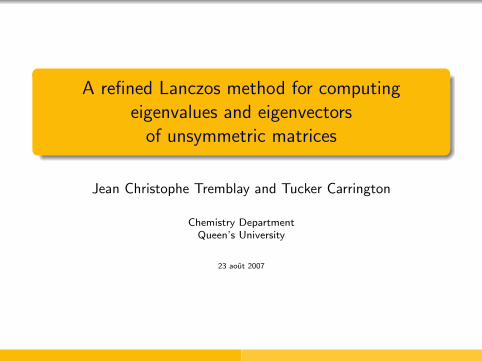
We want to solve the eigenvalue problem

GX(R) = X(R)Λ

We seek, first and foremost, an eigensolver that minimizes theamount of memory required to solve the problem.

For symmetric matrices the Lanczos algorithm withoutre-orthogonalization is a good choice.

only two vectors are stored in memory

Eigensolvers for unsymmetric matrices

For unsymmetric matrices the established methods are :

variants of the Arnoldi algorithm

the unsymmetric (or two-sided) Lanczos algorithm (ULA)

In this talk I present a method that in some sense is betterthan both.

What are the deficiencies of Arnoldi ?

It requires storing many vectors in memory. Every Arnoldivector is orthogonalized against all of the previous computedArnoldi vectors.

The CPU cost of the orthogonalization also increases with thenumber of iterations.

These problems are to some extent mitigated by using theimplicitly restarted Arnoldi (IRA) technique (ARPACK).Nevertheless, for large matrices it is not possible to useARPACK on a computer that does not have a lot of memory.ARPACK is best if one wants extremal eigenvalues.

What are the deficiencies of the ULA ?

In its primitive form it seldom yields accurate eigenvalues.

Re-biorthogonalization improves the accuracy but negates themethod’s memory advantage.

The new method (RULE) in a nutshell

No re-biorthogonalization of the Lanczos vectors ; regardlessof the number of required iterations only 4 Lanczos vectorsare stored in memory

The method may be used to compute either extremal orinterior eigenvalues

We use approximate right and left eigenvectors obtained fromthe ULA to build a projected matrix which we diagonalize

The take-home message

The RULE makes it possible to extract accurate eigenvaluesfrom large Krylov spaces.

It is a good alternative to ARPACK

if the matrix for which eigenvalues are desired is so large thatthe memory ARPACK requires exceeds that of the computerif one wishes interior eigenvalues.

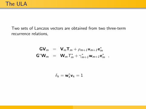
The ULA

Two sets of Lanczos vectors are obtained from two three-termrecurrence relations,

GVm = VmTm + ρm+1vm+1e∗mG∗Wm = WmT ∗m + γ∗m+1wm+1e∗m ,

δk = w∗kvk = 1

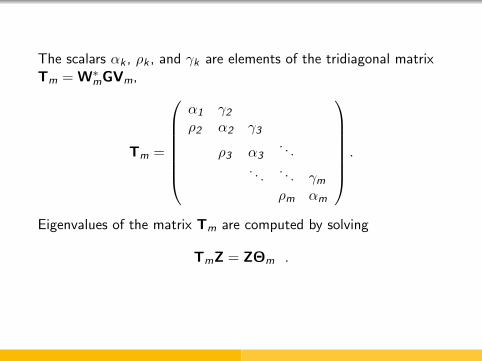
The scalars αk , ρk , and γk are elements of the tridiagonal matrixTm = W∗

mGVm,

Tm =

α1 γ2

ρ2 α2 γ3

ρ3 α3. . .

. . .. . . γm

ρm αm

.

Eigenvalues of the matrix Tm are computed by solving

TmZ = ZΘm .

The ULA does not work !

Roundoff errors lead to loss of biorthogonality of the Lanczosvectors.→ near but poor copies

it is not possible to find a Krylov subspace size m for which aneigenvalue of the matrix Tm accurately approximates aneigenvalue of the matrix G

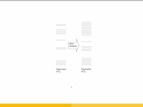
for each nearly converged eigenvalue of the matrix G there isa cluster of closely spaced eigenvalues of Tm, but the norm ofdifferences between eigenvalues in the cluster may be so largethat it is difficult to identify the cluster and impossible todetermine an accurate value for the eigenvalue

the width of the clusters increases with m

3

Eigenvalues of Tm

Eigenvalues of Tm

More iterations

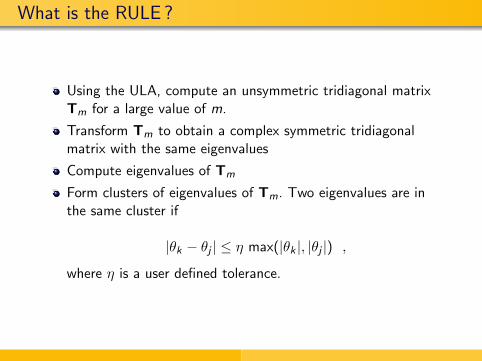
What is the RULE ?

Using the ULA, compute an unsymmetric tridiagonal matrixTm for a large value of m.

Transform Tm to obtain a complex symmetric tridiagonalmatrix with the same eigenvalues

Compute eigenvalues of Tm

Form clusters of eigenvalues of Tm. Two eigenvalues are inthe same cluster if

|θk − θj | ≤ η max(|θk |, |θj |) ,

where η is a user defined tolerance.

2

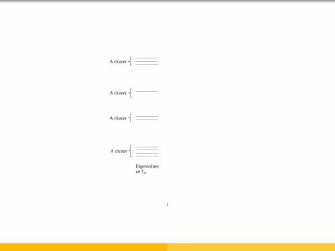
Eigenvalues of Tm

A cluster

A cluster

A cluster

A cluster

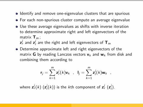
Identify and remove one-eigenvalue clusters that are spurious

For each non-spurious cluster compute an average eigenvalue

Use these average eigenvalues as shifts with inverse iterationto determine approximate right and left eigenvectors of thematrix Tm ;zjr and zj

l are the right and left eigenvectors of Tm

Determine approximate left and right eigenvectors of thematrix G by reading Lanczos vectors vk and wk from disk andcombining them according to

rj =m∑

k=1

zjr (k)vk , lj =

m∑k=1

zjl (k)wk ,

where zjr (k) (zj

l (k)) is the kth component of zjr (zj

l ).

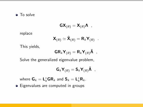
To solve

GX(R) = X(R)Λ ,

replaceX(R) ' X(R) = RkY(R) .

This yields,GRkY(R) = RkY(R)Λ ,

Solve the generalized eigenvalue problem,

GkY(R) = SkY(R)Λ ,

where Gk = L∗kGRk and Sk = L∗kRk .

Eigenvalues are computed in groups

How do we choose m ?

Increasing m does degrade the approximate eigenvectors so there isno need to carefully search for the best m. We choose a large valueof m, generate Lanczos vectors, and compute Gk . We compare theeigenvalues determined with those computed with a larger value ofm and increase m if necessary.

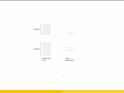
How do we choose η ?

If η is too small :

Several rj and lj vectors are nearly parallel.

This occurs if several of the clusters contain eigenvalues of thematrix Tm associated with one exact eigenvalue of the matrix G.

To minimize the near linear dependance of the vectors rj and lj and

to reduce the number of the {zjr , z

jl} pairs, we retain only pairs for

which Ritz values obtained from inverse iteration differ by morethan η max(|θmj

j |, |θmkk |).

4

Exact eigenvalues

Eigenvalues of Tm

A cluster

A cluster

A cluster

A cluster

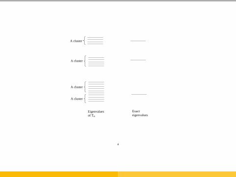
How do we choose η ?

If η is too large :

Eigenvalues of the matrix Tm associated with two or more exacteigenvalues will be lumped into a single cluster and one will misseigenvalues.

1

A cluster

A cluster

Exact eigenvalues

Eigenvalues of Tm

One could actually use the RULE with η = 0 (i.e. cluster width ofzero).

This would increase the number of {zjr , z

jl} pairs to compute and

make the calculation more costly.

We put η equal to be the square root of the machine precision.

Numerical experiments

TOLOSA matrices from the matrix market.

The largest matrix is 2000 × 2000.

The eigenvalues of interest are the three with the largest imaginaryparts.

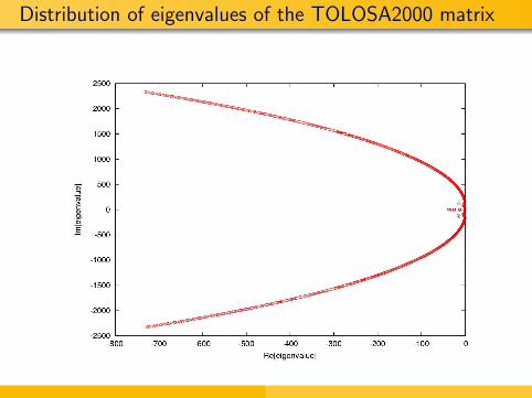
Distribution of eigenvalues of the TOLOSA2000 matrix

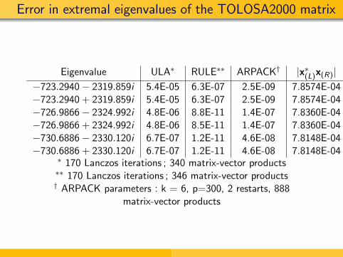
Error in extremal eigenvalues of the TOLOSA2000 matrix

Eigenvalue ULA∗ RULE∗∗ ARPACK† |x∗(L)x(R)|−723.2940− 2319.859i 5.4E-05 6.3E-07 2.5E-09 7.8574E-04−723.2940 + 2319.859i 5.4E-05 6.3E-07 2.5E-09 7.8574E-04−726.9866− 2324.992i 4.8E-06 8.8E-11 1.4E-07 7.8360E-04−726.9866 + 2324.992i 4.8E-06 8.5E-11 1.4E-07 7.8360E-04−730.6886− 2330.120i 6.7E-07 1.2E-11 4.6E-08 7.8148E-04−730.6886 + 2330.120i 6.7E-07 1.2E-11 4.6E-08 7.8148E-04

∗ 170 Lanczos iterations ; 340 matrix-vector products∗∗ 170 Lanczos iterations ; 346 matrix-vector products† ARPACK parameters : k = 6, p=300, 2 restarts, 888

matrix-vector products

A larger matrix - The AIRFOIL matrix

It is 23’560 × 23’560.

We focus on the eigenvalues of largest magnitude.

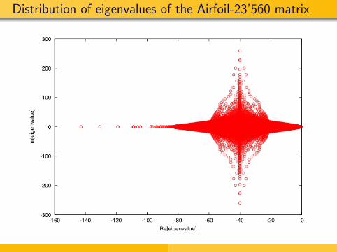
Distribution of eigenvalues of the Airfoil-23’560 matrix

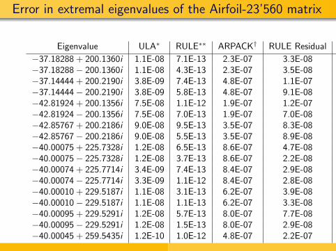
Error in extremal eigenvalues of the Airfoil-23’560 matrix

Eigenvalue ULA∗ RULE∗∗ ARPACK† RULE Residual |x∗(L)x(R)|−37.18288 + 200.1360i 1.1E-08 7.1E-13 2.3E-07 3.3E-08 0.21239−37.18288− 200.1360i 1.1E-08 4.3E-13 2.3E-07 3.5E-08 0.21239−37.14444 + 200.2190i 3.8E-09 7.4E-13 4.8E-07 1.1E-07 0.21716−37.14444− 200.2190i 3.8E-09 5.8E-13 4.8E-07 9.1E-08 0.21716−42.81924 + 200.1356i 7.5E-08 1.1E-12 1.9E-07 1.2E-07 0.21236−42.81924− 200.1356i 7.5E-08 7.0E-13 1.9E-07 7.0E-08 0.21236−42.85767 + 200.2186i 9.0E-08 9.5E-13 3.5E-07 8.3E-08 0.21713−42.85767− 200.2186i 9.0E-08 5.5E-13 3.5E-07 8.9E-08 0.21713−40.00075 + 225.7328i 1.2E-08 6.5E-13 8.6E-07 4.7E-08 0.26668−40.00075− 225.7328i 1.2E-08 3.7E-13 8.6E-07 2.2E-08 0.26668−40.00074 + 225.7714i 3.4E-09 7.4E-13 8.4E-07 2.9E-08 0.26530−40.00074− 225.7714i 3.3E-09 1.1E-12 8.4E-07 2.8E-08 0.26530−40.00010 + 229.5187i 1.1E-08 3.1E-13 6.2E-07 3.9E-08 0.22165−40.00010− 229.5187i 1.1E-08 1.1E-13 6.2E-07 3.3E-08 0.22165−40.00095 + 229.5291i 1.2E-08 5.7E-13 8.0E-07 7.7E-08 0.22236−40.00095− 229.5291i 1.2E-08 1.5E-13 8.0E-07 2.9E-08 0.22236−40.00045 + 259.5435i 1.2E-10 1.0E-12 4.8E-07 2.2E-07 0.41406−40.00045− 259.5435i 1.4E-10 7.6E-13 4.8E-07 8.7E-08 0.41406−40.00041 + 259.5534i 9.0E-11 6.9E-13 1.6E-06 1.9E-07 0.41406−40.00041− 259.5534i 1.6E-10 4.1E-13 1.6E-06 6.2E-08 0.41406

∗ 125 Lanczos iterations ; 250 matrix-vector products∗∗ 125 Lanczos iterations ; 270 matrix-vector products† ARPACK parameters : k = 20, p=50, 6 restarts, 172

matrix-vector products

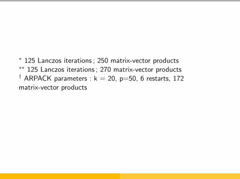
∗ 125 Lanczos iterations ; 250 matrix-vector products∗∗ 125 Lanczos iterations ; 270 matrix-vector products† ARPACK parameters : k = 20, p=50, 6 restarts, 172matrix-vector products

Interior eigenalues - The PDE matrix

Obtained from matrix market.

It is 2961 × 2961.

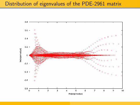
Distribution of eigenvalues of the PDE-2961 matrix

The approximate eigenvectors we use are those whosecorresponding eigenvalues lie in a rectangular box of width 0.5 andheight 0.1i centered at a target value of 8.3 + 0.35i .

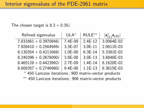
Interior eigenvalues of the PDE-2961 matrix

The chosen target is 8.3 + 0.35i .

Refined eigenvalue ULA∗ RULE∗∗ |x∗(L)x(R)|7.831661 + 0.3970848i 7.4E-09 2.4E-12 3.0064E-027.928410 + 0.2564949i 3.3E-07 3.0E-11 2.0611E-038.130354 + 0.4211668i 1.0E-08 6.3E-14 5.3381E-028.240396 + 0.2678090i 3.8E-08 3.0E-13 3.8846E-038.465128 + 0.4423992i 2.7E-09 1.4E-14 8.1620E-028.600357 + 0.2746980i 9.4E-08 1.1E-13 6.3615E-03∗ 450 Lanczos iterations ; 900 matrix-vector products∗∗ 450 Lanczos iterations ; 906 matrix-vector products

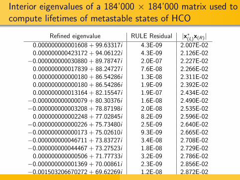
Interior eigenvalues of a 184’000 × 184’000 matrix used tocompute lifetimes of metastable states of HCO

Refined eigenvalue RULE Residual |x∗(L)x(R)|0.000000000001608 + 99.63317i 4.3E-09 2.007E-020.000000000423172 + 94.06122i 4.3E-09 2.126E-02−0.000000000030880 + 89.78747i 2.0E-07 2.227E-02

0.000000000017839 + 88.24727i 7.6E-08 2.266E-020.000000000000180 + 86.54286i 1.3E-08 2.311E-020.000000000000180 + 86.54286i 1.9E-09 2.392E-020.000000000013164 + 82.15547i 1.9E-07 2.434E-02−0.000000000000079 + 80.30376i 1.6E-08 2.490E-02−0.000000000003208 + 78.87198i 2.0E-08 2.535E-02

0.000000000002248 + 77.02845i 8.2E-09 2.596E-02−0.000000000000226 + 75.73480i 2.5E-09 2.640E-02−0.000000000000173 + 75.02610i 9.3E-09 2.665E-02−0.000000000046711 + 73.83727i 3.4E-08 2.708E-02−0.000000000044467 + 73.27523i 1.8E-08 2.729E-02

0.000000000000506 + 71.77733i 3.2E-09 2.786E-02−0.000000000001369 + 70.00861i 2.3E-09 2.856E-02−0.001503206670272 + 69.62269i 1.2E-08 2.872E-02−0.001616758817681 + 69.28458i 1.1E-07 2.886E-02−0.001799287965362 + 68.97843i 7.1E-07 2.899E-02

0.000000192654410 + 68.91187i 1.1E-06 2.902E-02−0.001958836517186 + 68.69687i 4.1E-06 2.910E-02

Number of unsymmetric Lanczos iterations : 3000

Conclusion

A simple refinement (the RULE) makes it possible to extractaccurate eigenvalues from the Krylov subspaces obtained fromthe ULA.

The RULE makes it possible to use large Krylov subspaceswithout storing a large number of vectors in memory andre-biorthogonalizing Lanczos vectors.

It can therefore be used to compute many eigenvalues of verylarge matrices.

The refinement is inexpensive. Eigenvalues are computed ingroups of about 20. For each group of 20 the cost of therefinement is only 20 additional matrix-vector products.

This work has been supported by theNatural Sciences and EngineeringResearch Council of Canada