Variational Methods

Zoubin Ghahramani

zoubin@cs.cmu.edu

http://www.gatsby.ucl.ac.uk

Statistical Approaches to Learning and DiscoveryCarnegie Mellon University

April 2003

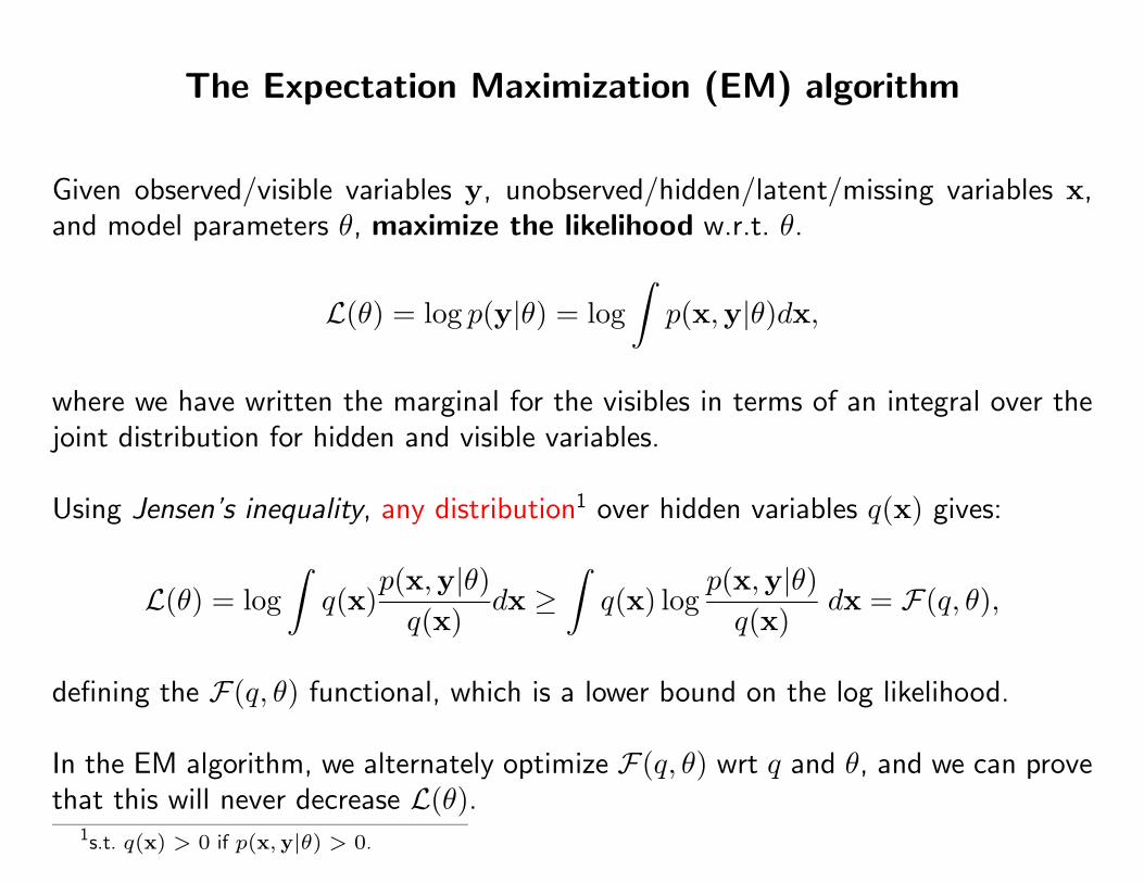
The Expectation Maximization (EM) algorithm

Given observed/visible variables y, unobserved/hidden/latent/missing variables x,and model parameters θ, maximize the likelihood w.r.t. θ.

L(θ) = log p(y|θ) = log∫p(x,y|θ)dx,

where we have written the marginal for the visibles in terms of an integral over thejoint distribution for hidden and visible variables.

Using Jensen’s inequality, any distribution1 over hidden variables q(x) gives:

L(θ) = log∫q(x)

p(x,y|θ)q(x)

dx ≥∫q(x) log

p(x,y|θ)q(x)

dx = F(q, θ),

defining the F(q, θ) functional, which is a lower bound on the log likelihood.

In the EM algorithm, we alternately optimize F(q, θ) wrt q and θ, and we can provethat this will never decrease L(θ).

1s.t. q(x) > 0 if p(x, y|θ) > 0.

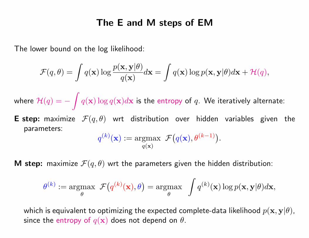
The E and M steps of EM

The lower bound on the log likelihood:

F(q, θ) =∫q(x) log

p(x,y|θ)q(x)

dx =∫q(x) log p(x,y|θ)dx +H(q),

where H(q) = −∫q(x) log q(x)dx is the entropy of q. We iteratively alternate:

E step: maximize F(q, θ) wrt distribution over hidden variables given theparameters:

q(k)(x) := argmaxq(x)

F(q(x), θ(k−1)

).

M step: maximize F(q, θ) wrt the parameters given the hidden distribution:

θ(k) := argmaxθ

F(q(k)(x), θ

)= argmax

θ

∫q(k)(x) log p(x,y|θ)dx,

which is equivalent to optimizing the expected complete-data likelihood p(x,y|θ),since the entropy of q(x) does not depend on θ.

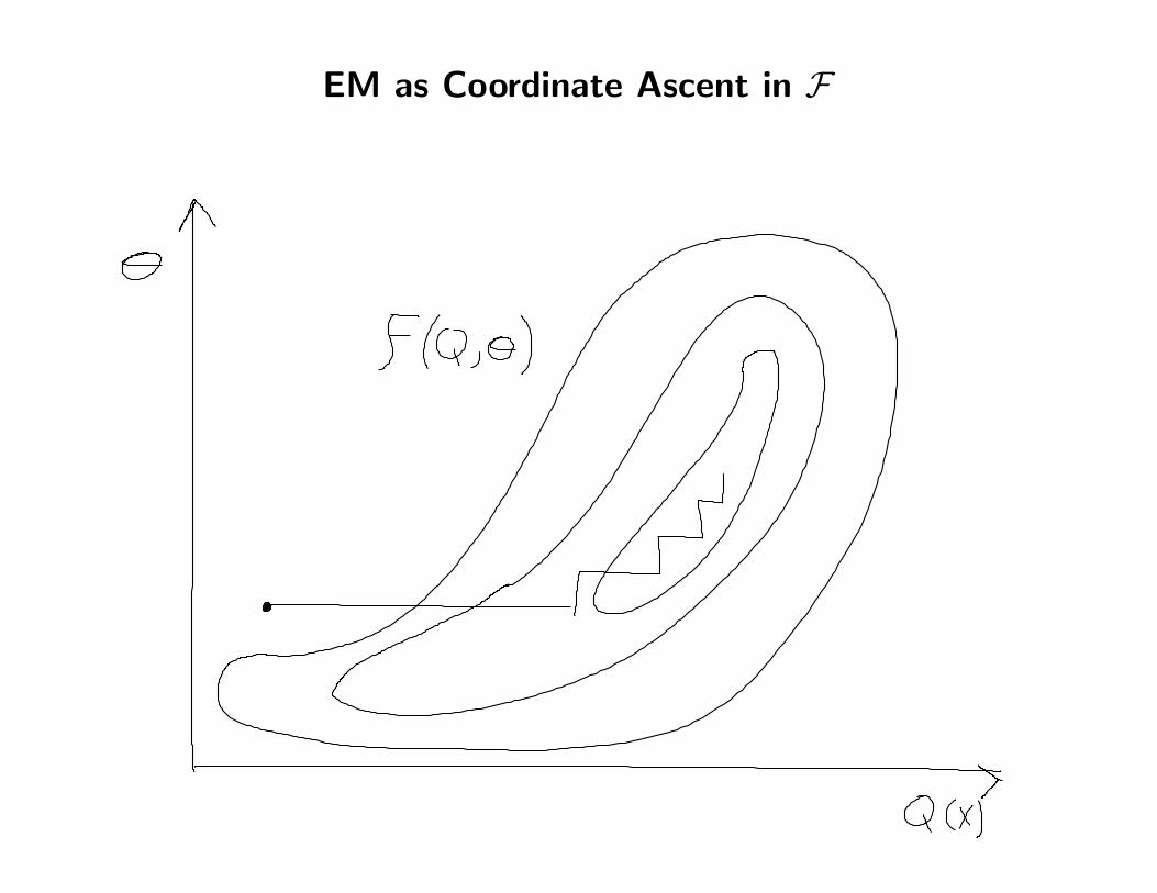
EM as Coordinate Ascent in F

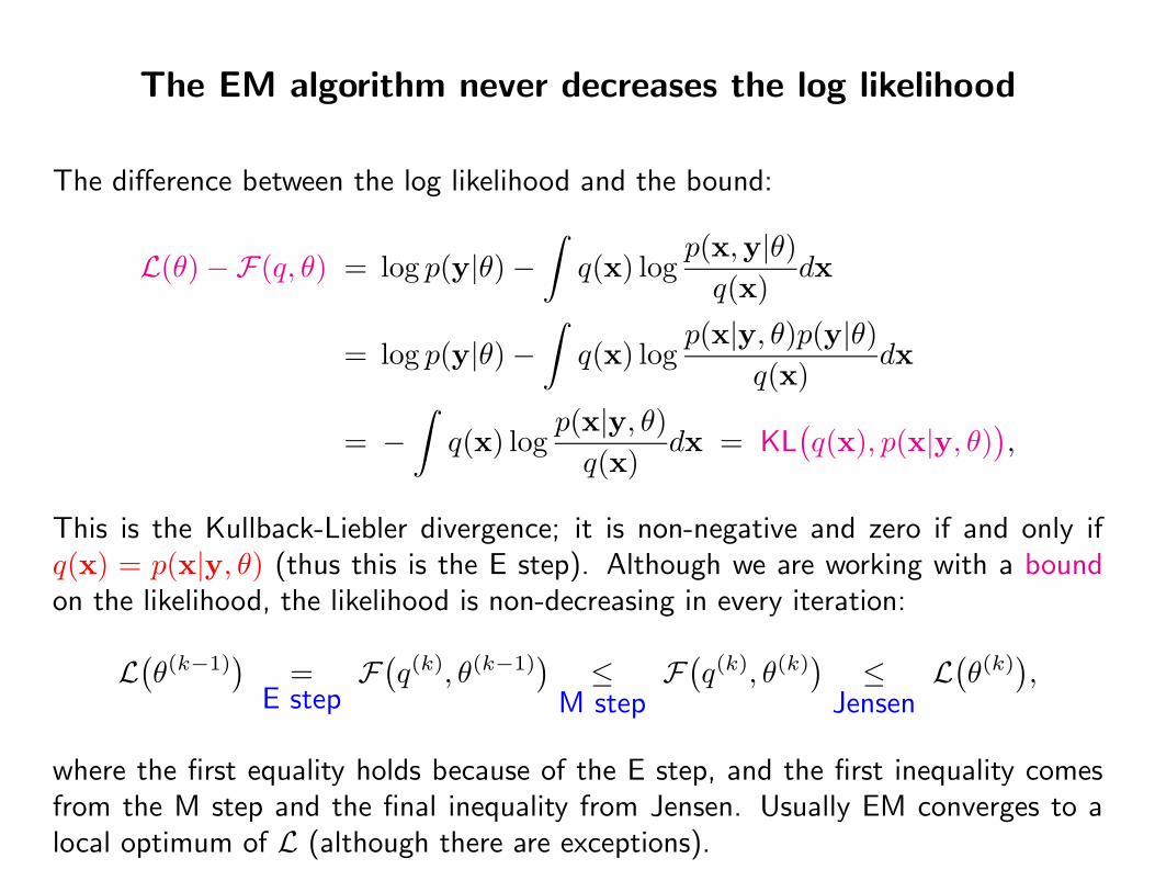
The EM algorithm never decreases the log likelihood

The difference between the log likelihood and the bound:

L(θ)−F(q, θ) = log p(y|θ)−∫q(x) log

p(x,y|θ)q(x)

dx

= log p(y|θ)−∫q(x) log

p(x|y, θ)p(y|θ)q(x)

dx

= −∫q(x) log

p(x|y, θ)q(x)

dx = KL(q(x), p(x|y, θ)

),

This is the Kullback-Liebler divergence; it is non-negative and zero if and only ifq(x) = p(x|y, θ) (thus this is the E step). Although we are working with a boundon the likelihood, the likelihood is non-decreasing in every iteration:

L(θ(k−1)

)=

E stepF(q(k), θ(k−1)

)≤

M stepF(q(k), θ(k)

)≤

JensenL(θ(k)

),

where the first equality holds because of the E step, and the first inequality comesfrom the M step and the final inequality from Jensen. Usually EM converges to alocal optimum of L (although there are exceptions).

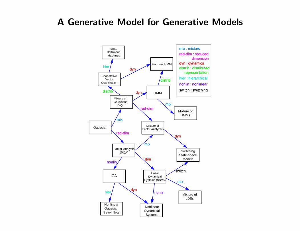
A Generative Model for Generative Models

Gaussian

Factor Analysis (PCA)

Mixture of Factor Analyzers

Mixture of Gaussians

(VQ)

Cooperative Vector

Quantization

SBN, Boltzmann Machines

Factorial HMM

HMM

Mixture of

HMMs

Switching State-space

Models

ICALinear

Dynamical Systems (SSMs)

Mixture of LDSs

Nonlinear Dynamical Systems

Nonlinear Gaussian

Belief Nets

mix

mix

mix

switch

red-dim

red-dim

dyn

dyn

dyn

dyn

dyn

mix

distrib

hier

nonlinhier

nonlin

distrib

mix : mixture

red-dim : reduced dimension dyn : dynamics distrib : distributed representation

hier : hierarchical

nonlin : nonlinear

switch : switching

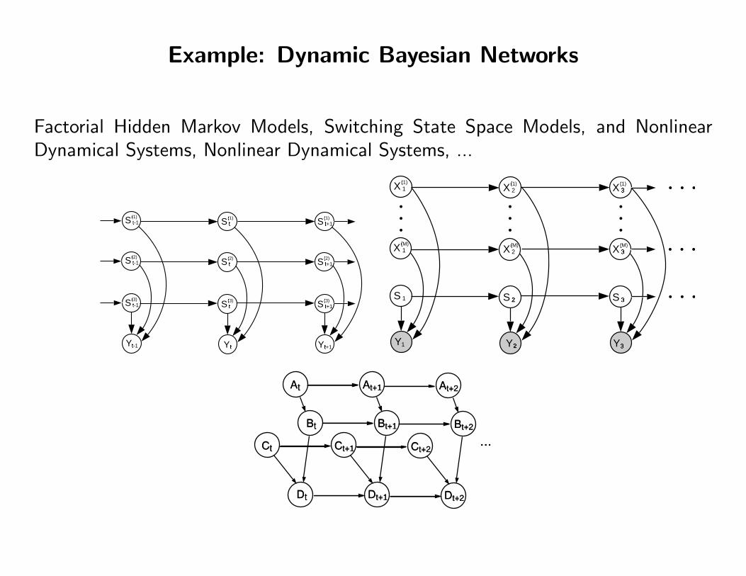
Example: Dynamic Bayesian Networks

Factorial Hidden Markov Models, Switching State Space Models, and NonlinearDynamical Systems, Nonlinear Dynamical Systems, ...

S(1)�

t�

S(2)�

t�

S(3)�

t�

Yt�

S(1)�

t+1�

S(2)�

t+1�

S(3)�

t+1�

Yt+1�

S(1)�

t-1�

S(2)�

t-1�

S(3)�

t-1�

Yt-1�

X(M)�

2

S 2�

Y2�

X(M)�

3�

S 3�

Y3�

X(M)�

1

S 1

Y1

X(1)�

2 X(1)�

3�X(1)

�

1

At

Dt

Ct

Bt

At+1

Dt+1

Ct+1

Bt+1

...

At+2

Dt+2

Ct+2

Bt+2

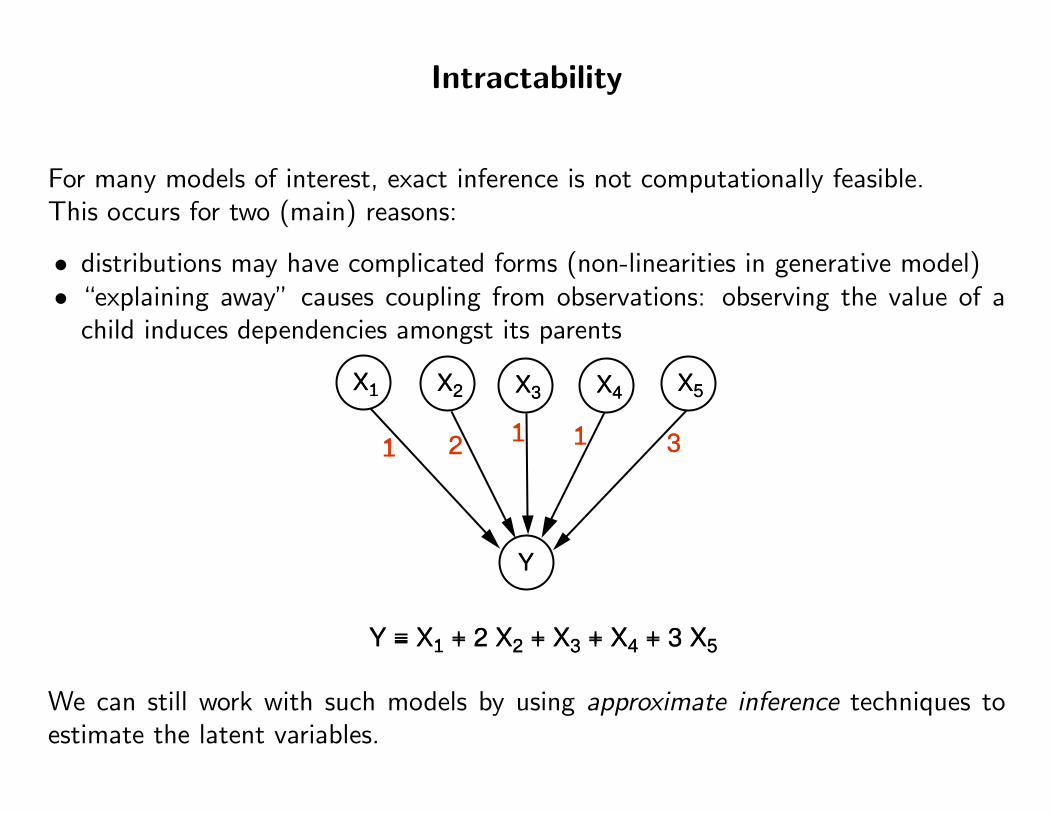
Intractability

For many models of interest, exact inference is not computationally feasible.This occurs for two (main) reasons:

• distributions may have complicated forms (non-linearities in generative model)• “explaining away” causes coupling from observations: observing the value of a

child induces dependencies amongst its parents

Y

X3 X4X1 X5X2

1 2 311

Y = X1 + 2 X2 + X3 + X4 + 3 X5

We can still work with such models by using approximate inference techniques toestimate the latent variables.

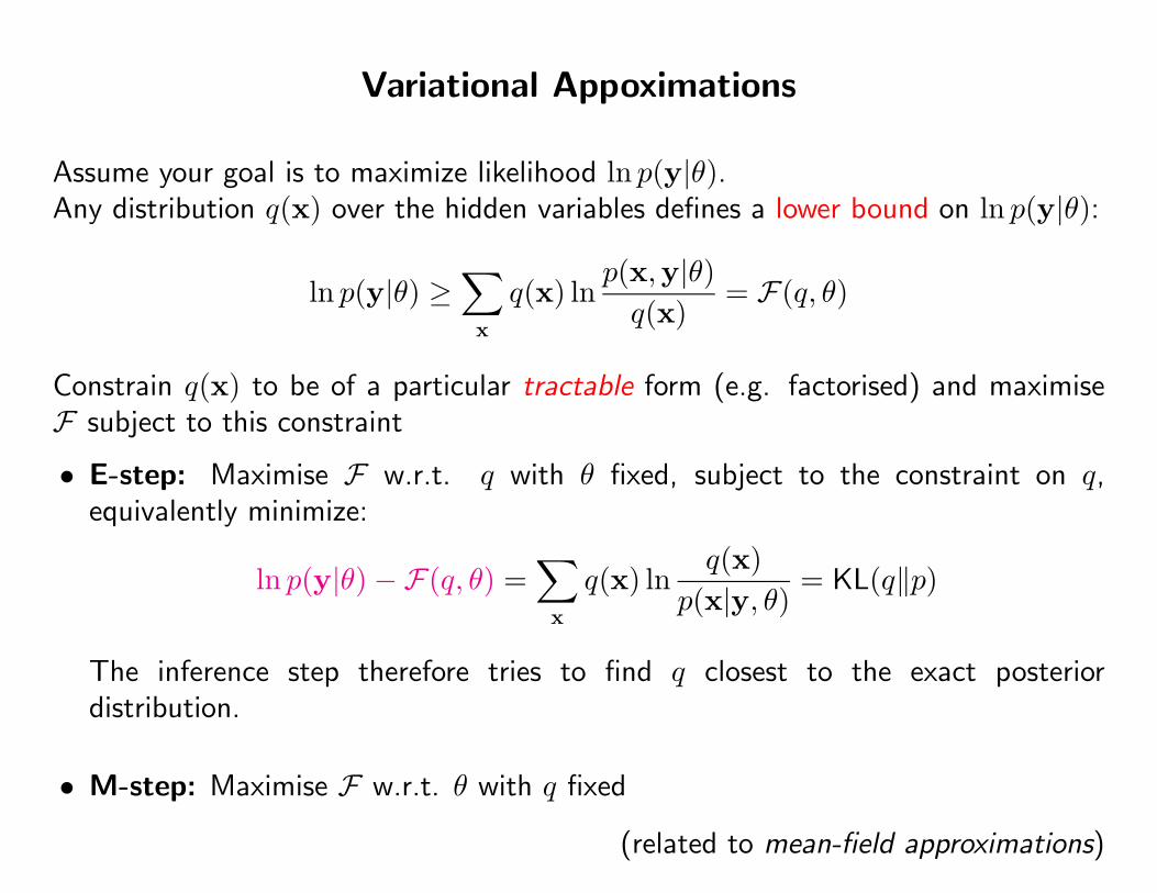
Variational Appoximations

Assume your goal is to maximize likelihood ln p(y|θ).Any distribution q(x) over the hidden variables defines a lower bound on ln p(y|θ):

ln p(y|θ) ≥∑

x

q(x) lnp(x,y|θ)q(x)

= F(q, θ)

Constrain q(x) to be of a particular tractable form (e.g. factorised) and maximiseF subject to this constraint

• E-step: Maximise F w.r.t. q with θ fixed, subject to the constraint on q,equivalently minimize:

ln p(y|θ)−F(q, θ) =∑

x

q(x) lnq(x)

p(x|y, θ)= KL(q‖p)

The inference step therefore tries to find q closest to the exact posteriordistribution.

• M-step: Maximise F w.r.t. θ with q fixed

(related to mean-field approximations)

Variational Approximations for Bayesian Learning

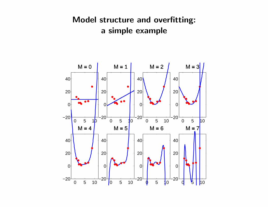
Model structure and overfitting:a simple example

0 5 10−20

0

20

40

M = 0

0 5 10−20

0

20

40

M = 1

0 5 10−20

0

20

40

M = 2

0 5 10−20

0

20

40

M = 3

0 5 10−20

0

20

40

M = 4

0 5 10−20

0

20

40

M = 5

0 5 10−20

0

20

40

M = 6

0 5 10−20

0

20

40

M = 7

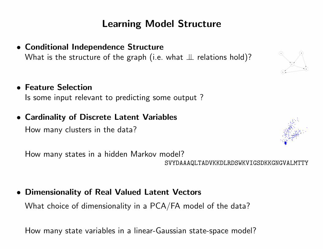
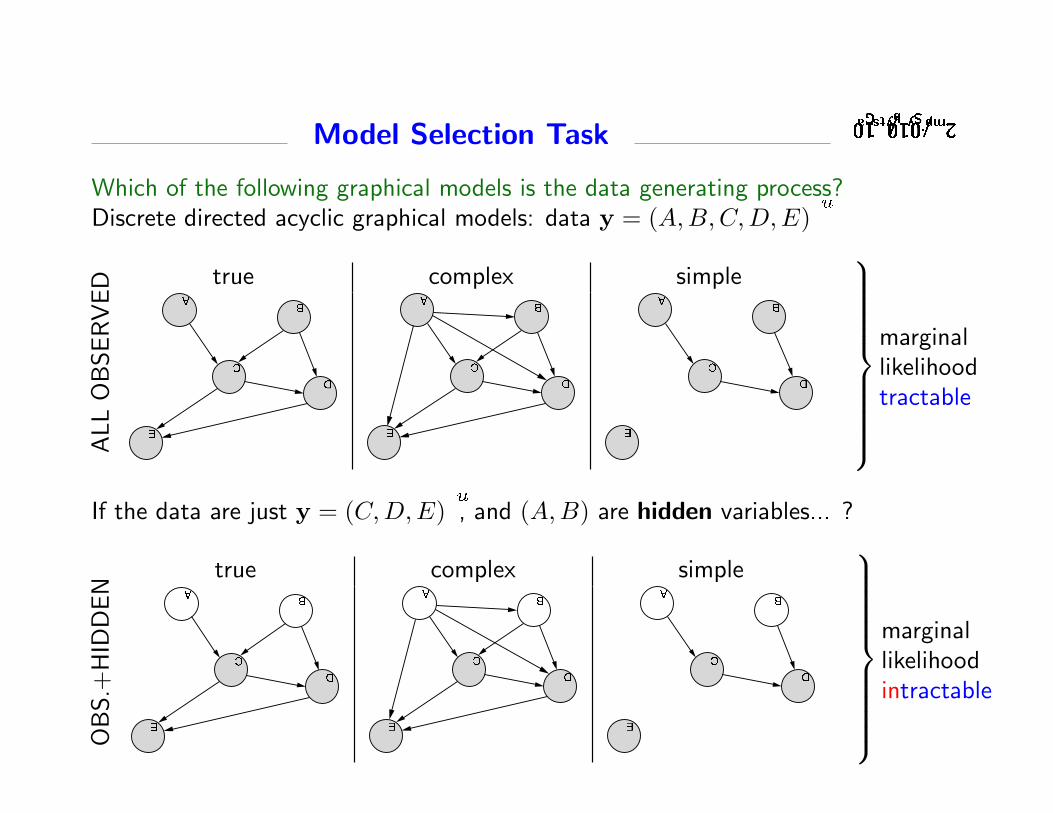
Learning Model Structure

• Conditional Independence StructureWhat is the structure of the graph (i.e. what ⊥⊥ relations hold)?

A

C

B

D

E

• Feature SelectionIs some input relevant to predicting some output ?

• Cardinality of Discrete Latent Variables

How many clusters in the data?

How many states in a hidden Markov model?SVYDAAAQLTADVKKDLRDSWKVIGSDKKGNGVALMTTY

• Dimensionality of Real Valued Latent Vectors

What choice of dimensionality in a PCA/FA model of the data?

How many state variables in a linear-Gaussian state-space model?

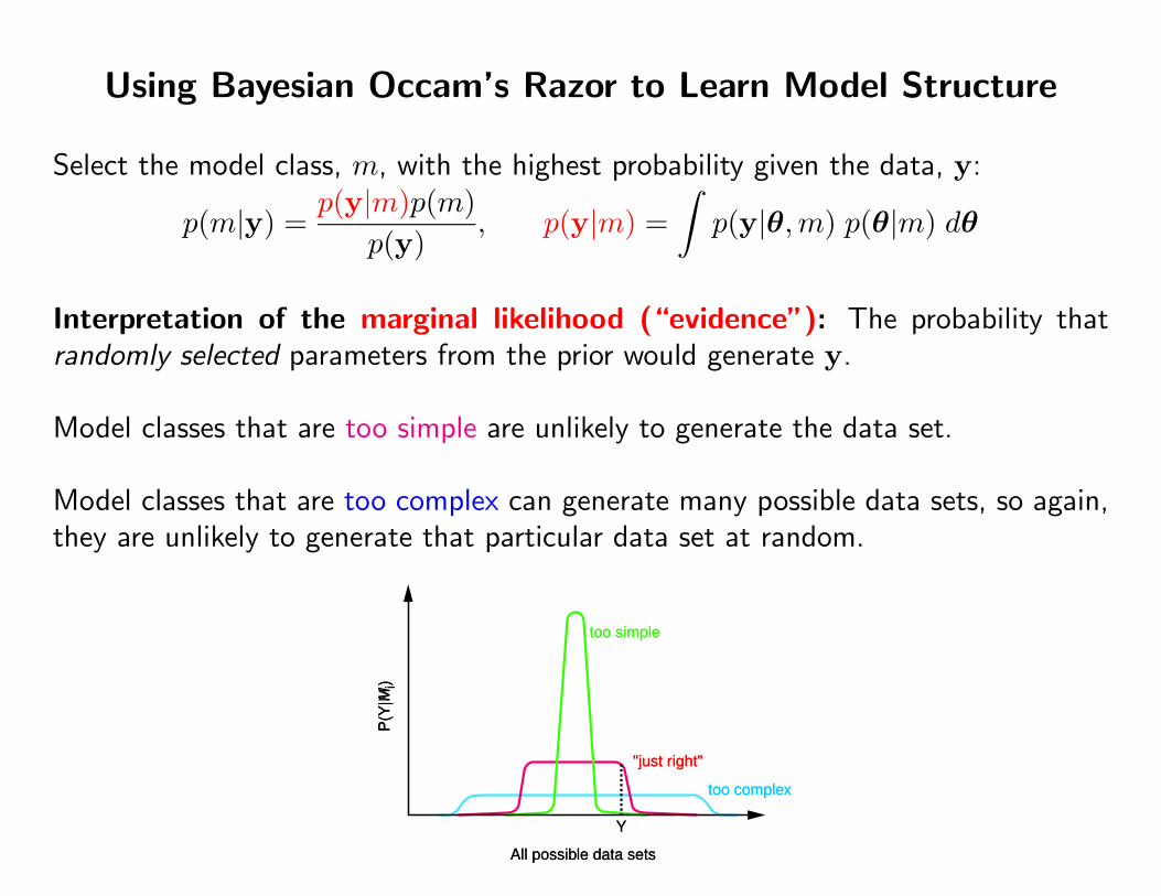
Using Bayesian Occam’s Razor to Learn Model Structure

Select the model class, m, with the highest probability given the data, y:

p(m|y) =p(y|m)p(m)

p(y), p(y|m) =

∫p(y|θ,m) p(θ|m) dθ

Interpretation of the marginal likelihood (“evidence”): The probability thatrandomly selected parameters from the prior would generate y.

Model classes that are too simple are unlikely to generate the data set.

Model classes that are too complex can generate many possible data sets, so again,they are unlikely to generate that particular data set at random.

too simple

too complex

"just right"

All possible data sets

P(Y

|Mi)

Y

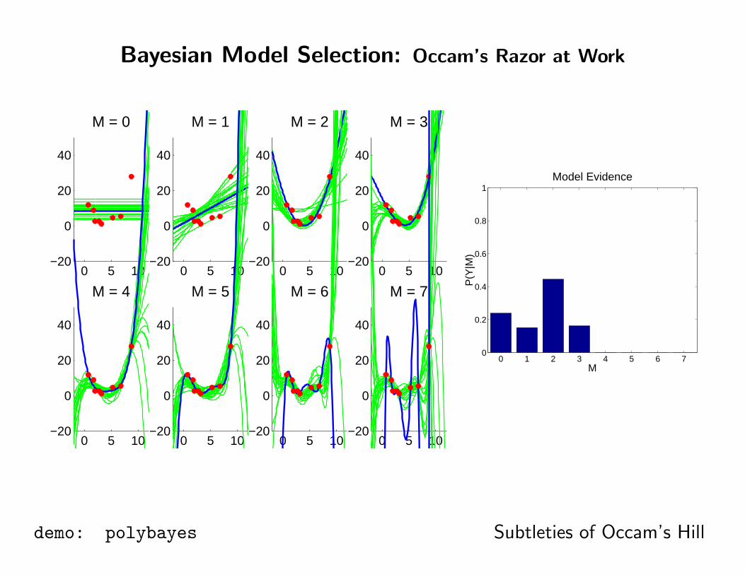
Bayesian Model Selection: Occam’s Razor at Work

0 5 10−20

0

20

40

M = 0

0 5 10−20

0

20

40

M = 1

0 5 10−20

0

20

40

M = 2

0 5 10−20

0

20

40

M = 3

0 5 10−20

0

20

40

M = 4

0 5 10−20

0

20

40

M = 5

0 5 10−20

0

20

40

M = 6

0 5 10−20

0

20

40

M = 7

0 1 2 3 4 5 6 70

0.2

0.4

0.6

0.8

1

M

P(Y

|M)

Model Evidence

demo: polybayes Subtleties of Occam’s Hill

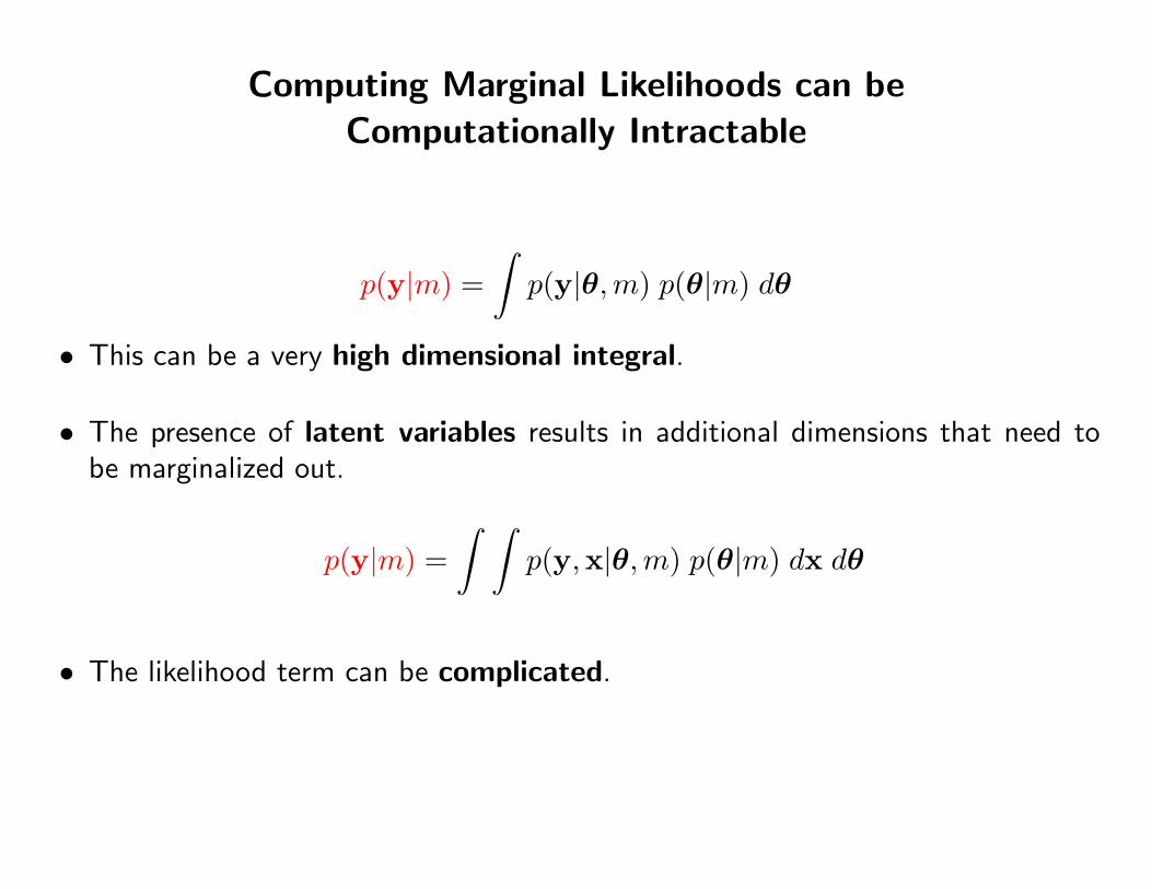
Computing Marginal Likelihoods can beComputationally Intractable

p(y|m) =∫p(y|θ,m) p(θ|m) dθ

• This can be a very high dimensional integral.

• The presence of latent variables results in additional dimensions that need tobe marginalized out.

p(y|m) =∫ ∫

p(y,x|θ,m) p(θ|m) dx dθ

• The likelihood term can be complicated.

Practical Bayesian approaches

• Laplace approximations:

– Appeals to asymptotic normality to make a Gaussian approximation about theposterior mode of the parameters.

• Large sample approximations (e.g. BIC).

• Markov chain Monte Carlo methods (MCMC):

– converge to the desired distribution in the limit, but:– many samples are required to ensure accuracy.– sometimes hard to assess convergence and reliably compute marginal likelihood.

• Variational approximations...

Note: other deterministic approximations are also available now: e.g. Bethe/Kikuchiapproximations, Expectation Propagation, Tree-based reparameterizations.

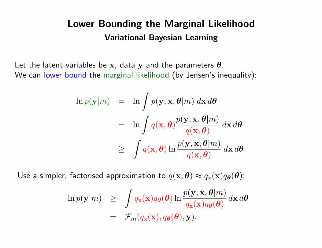
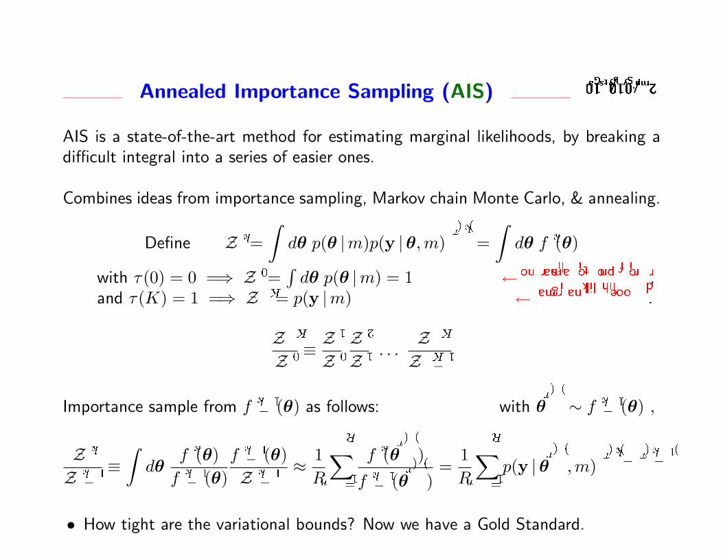
Lower Bounding the Marginal Likelihood

Variational Bayesian Learning

Let the latent variables be x, data y and the parameters θ.We can lower bound the marginal likelihood (by Jensen’s inequality):

ln p(y|m) = ln∫p(y,x,θ|m) dx dθ

= ln∫q(x,θ)

p(y,x,θ|m)q(x,θ)

dx dθ

≥∫q(x,θ) ln

p(y,x,θ|m)q(x,θ)

dx dθ.

Use a simpler, factorised approximation to q(x,θ) ≈ qx(x)qθ(θ):

ln p(y|m) ≥∫qx(x)qθ(θ) ln

p(y,x,θ|m)qx(x)qθ(θ)

dx dθ

= Fm(qx(x), qθ(θ),y).

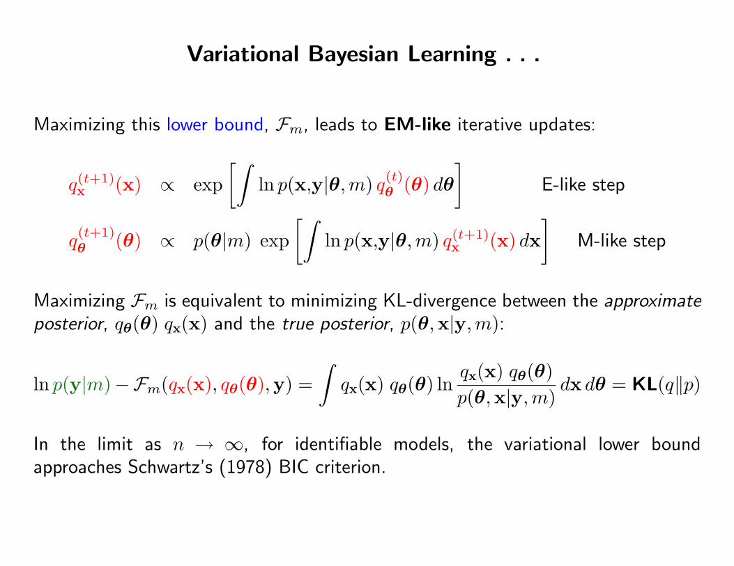
Variational Bayesian Learning . . .

Maximizing this lower bound, Fm, leads to EM-like iterative updates:

q(t+1)x (x) ∝ exp

[∫ln p(x,y|θ,m) q(t)

θ (θ) dθ]

E-like step

q(t+1)θ (θ) ∝ p(θ|m) exp

[∫ln p(x,y|θ,m) q(t+1)

x (x) dx]

M-like step

Maximizing Fm is equivalent to minimizing KL-divergence between the approximateposterior, qθ(θ) qx(x) and the true posterior, p(θ,x|y,m):

ln p(y|m)−Fm(qx(x), qθ(θ),y) =∫qx(x) qθ(θ) ln

qx(x) qθ(θ)p(θ,x|y,m)

dx dθ = KL(q‖p)

In the limit as n → ∞, for identifiable models, the variational lower boundapproaches Schwartz’s (1978) BIC criterion.

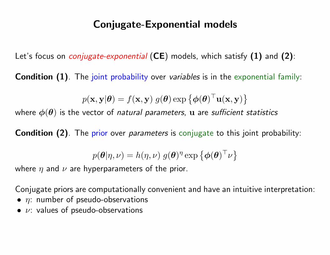
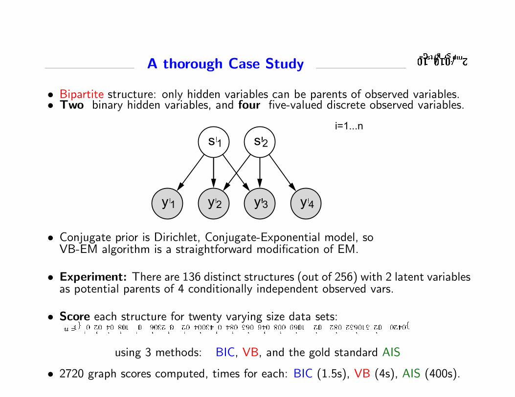
Conjugate-Exponential models

Let’s focus on conjugate-exponential (CE) models, which satisfy (1) and (2):

Condition (1). The joint probability over variables is in the exponential family:

p(x,y|θ) = f(x,y) g(θ) exp{φ(θ)>u(x,y)

}where φ(θ) is the vector of natural parameters, u are sufficient statistics

Condition (2). The prior over parameters is conjugate to this joint probability:

p(θ|η, ν) = h(η, ν) g(θ)η exp{φ(θ)>ν

}where η and ν are hyperparameters of the prior.

Conjugate priors are computationally convenient and have an intuitive interpretation:• η: number of pseudo-observations• ν: values of pseudo-observations

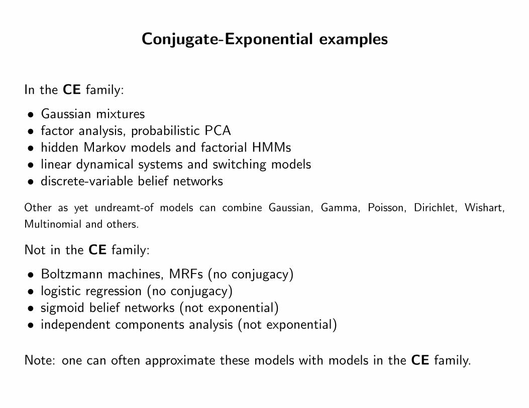
Conjugate-Exponential examples

In the CE family:

• Gaussian mixtures• factor analysis, probabilistic PCA• hidden Markov models and factorial HMMs• linear dynamical systems and switching models• discrete-variable belief networks

Other as yet undreamt-of models can combine Gaussian, Gamma, Poisson, Dirichlet, Wishart,

Multinomial and others.

Not in the CE family:

• Boltzmann machines, MRFs (no conjugacy)• logistic regression (no conjugacy)• sigmoid belief networks (not exponential)• independent components analysis (not exponential)

Note: one can often approximate these models with models in the CE family.

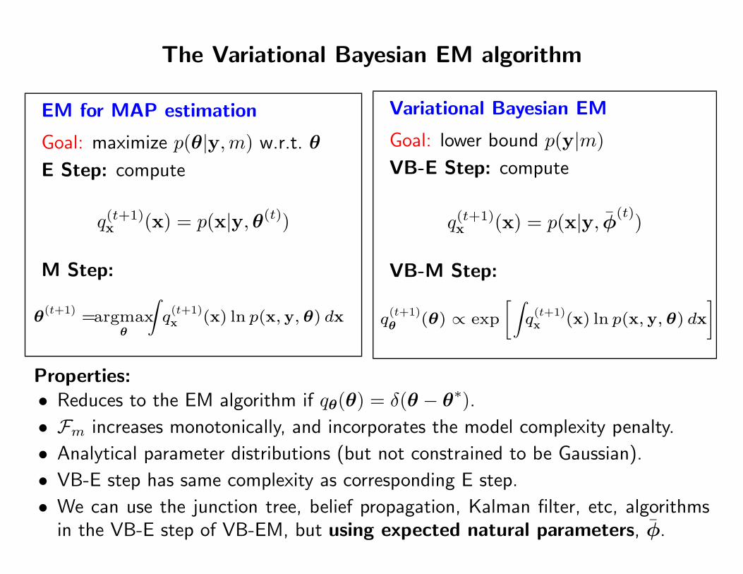
The Variational Bayesian EM algorithm

EM for MAP estimation

Goal: maximize p(θ|y,m) w.r.t. θ

E Step: compute

q(t+1)x (x) = p(x|y,θ(t))

M Step:

θ(t+1)

=argmaxθ

∫q

(t+1)x (x) ln p(x, y, θ) dx

Variational Bayesian EM

Goal: lower bound p(y|m)VB-E Step: compute

q(t+1)x (x) = p(x|y, φ(t))

VB-M Step:

q(t+1)θ (θ) ∝ exp

[∫q

(t+1)x (x) ln p(x, y, θ) dx

]

Properties:• Reduces to the EM algorithm if qθ(θ) = δ(θ − θ∗).

• Fm increases monotonically, and incorporates the model complexity penalty.

• Analytical parameter distributions (but not constrained to be Gaussian).

• VB-E step has same complexity as corresponding E step.

• We can use the junction tree, belief propagation, Kalman filter, etc, algorithmsin the VB-E step of VB-EM, but using expected natural parameters, φ.

Variational Bayesian EM

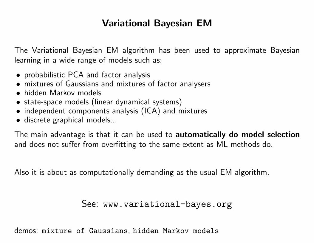
The Variational Bayesian EM algorithm has been used to approximate Bayesianlearning in a wide range of models such as:

• probabilistic PCA and factor analysis• mixtures of Gaussians and mixtures of factor analysers• hidden Markov models• state-space models (linear dynamical systems)• independent components analysis (ICA) and mixtures• discrete graphical models...

The main advantage is that it can be used to automatically do model selectionand does not suffer from overfitting to the same extent as ML methods do.

Also it is about as computationally demanding as the usual EM algorithm.

See: www.variational-bayes.org

demos: mixture of Gaussians, hidden Markov models

��� �� ��� � � ��� � � � �

�

� �

��

�

� �

��

�

� �

��

�

�

� �

��

�

� �

��

�

� �

��

�

��� �� ��� � � ��� � � � �

�

� �

� � �

� � �� ��� � � � � � � � ��� � � � � � � � � �� ��� � � � � � � ��� �� � � � � � � � � ��� � � � � � � � � � � ��� � � � ��� � � � ��� � � � ��� �� � ��� � � � � � �

��� �� ��� � � ��� � � � �

� � � � ��

� �� � �� ���� � �� � � � ��� �� � �

�� �! � �� � ��" # ��$ � � %

�

&

�

'

&

&

� &��( �

� &

�

� &

�

� &

� &

� &

)

( * &

���( �

� &�( �

)

( * &

��( � � � � � � � � & �

��� �� ��� � � ��� � � � �

� ��

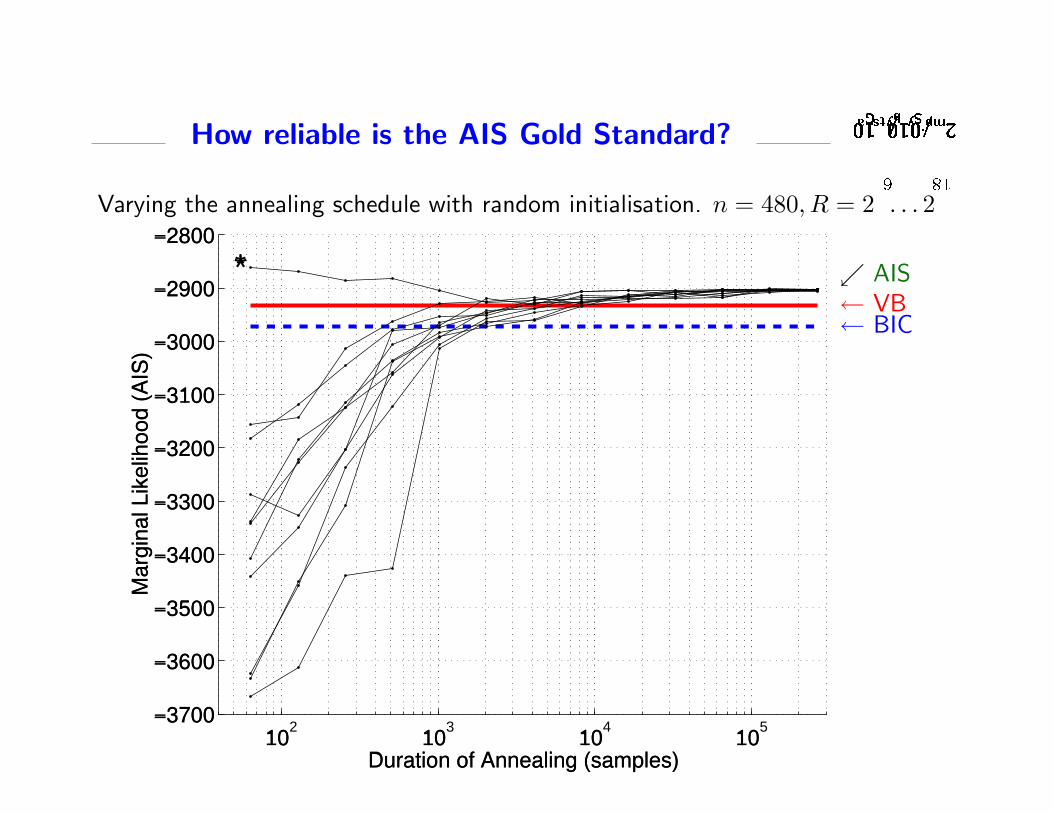
102

103

104

105

−3700

−3600

−3500

−3400

−3300

−3200

−3100

−3000

−2900

−2800

Duration of Annealing (samples)

Mar

gina

l Lik

elih

ood

(AIS

)

*

��� �� ��� � � ��� � � � �

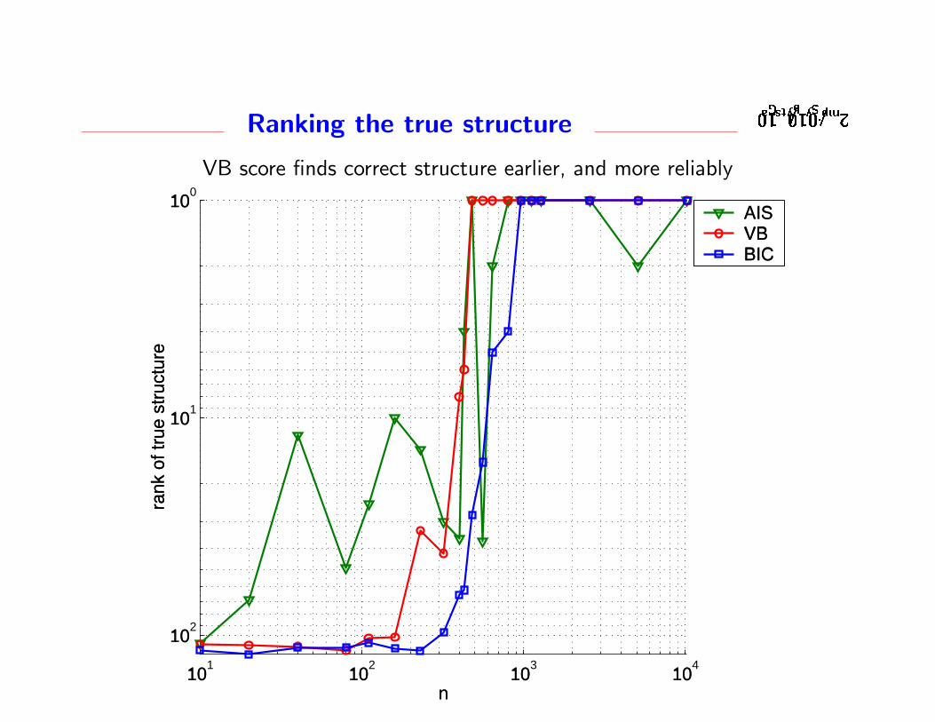
101

102

103

104

100

101

102

n

rank

of t

rue

stru

ctur

e

AISVBBIC

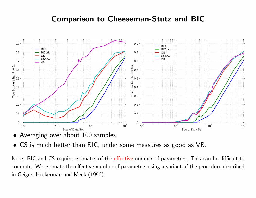
Comparison to Cheeseman-Stutz and BIC

101

102

103

104

0

0.1

0.2

0.3

0.4

0.5

0.6

0.7

0.8

0.9

Size of Data Set

Tru

e S

truc

ture

has

P>

0.01

BICBICpriorCSCSnewVB

101

102

103

104

0

0.1

0.2

0.3

0.4

0.5

0.6

0.7

0.8

0.9

Size of Data SetT

rue

Str

uctu

re h

as P

>0.

5

BICBICpriorCSCSnewVB

• Averaging over about 100 samples.

• CS is much better than BIC, under some measures as good as VB.

Note: BIC and CS require estimates of the effective number of parameters. This can be difficult to

compute. We estimate the effective number of parameters using a variant of the procedure described

in Geiger, Heckerman and Meek (1996).

Summary and Conclusions

• EM can be interpreted as a lower bound maximization algorithm.

• For many models of interest the E step is intractable.

• For such models an approximate E step can be used in a variational lower boundoptimization algorithm.

• This lower bound idea can also be used to do variational Bayesian learning.

• Bayesian learning embodies automatic Occam’s razor via the marginal likelihood.

• This makes it possible to avoid overfitting and select models.

Appendix

Appendix

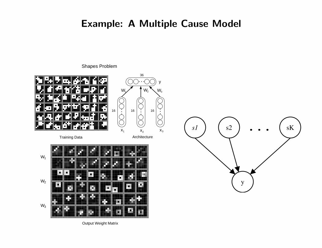
Example: A Multiple Cause Model

Training Data

Output Weight Matrix

Shapes Problem

y

x1 x2 x3

W1 W3W2

. . .

. . .

. . .

. . .

36

16 16 16

Architecture

W1

W2

W3

s1 s2 sK

y

...

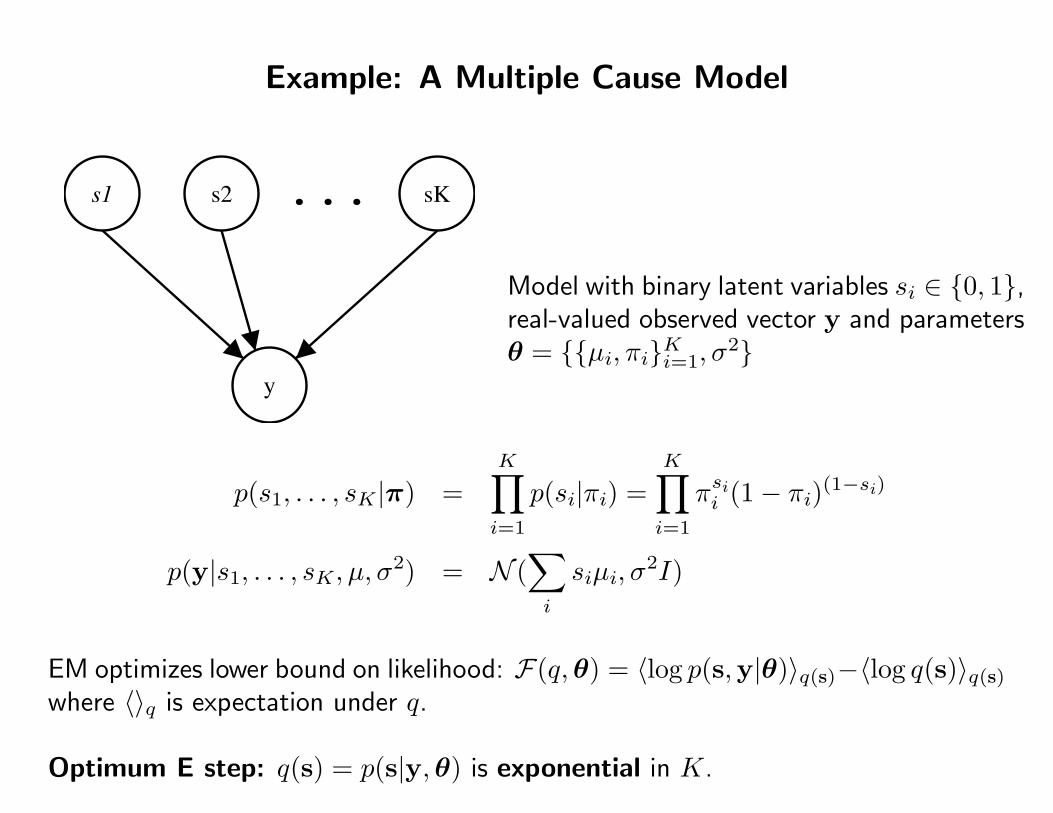
Example: A Multiple Cause Model

s1 s2 sK

y

...

Model with binary latent variables si ∈ {0, 1},real-valued observed vector y and parametersθ = {{µi, πi}Ki=1, σ

2}

p(s1, . . . , sK|π) =K∏i=1

p(si|πi) =K∏i=1

πsii (1− πi)(1−si)

p(y|s1, . . . , sK, µ, σ2) = N (

∑i

siµi, σ2I)

EM optimizes lower bound on likelihood: F(q,θ) = 〈log p(s,y|θ)〉q(s)−〈log q(s)〉q(s)where 〈〉q is expectation under q.

Optimum E step: q(s) = p(s|y,θ) is exponential in K.

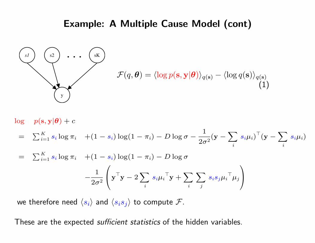
Example: A Multiple Cause Model (cont)

s1 s2 sK

y

...

F(q,θ) = 〈log p(s,y|θ)〉q(s) − 〈log q(s)〉q(s)(1)

log p(s, y|θ) + c

=∑K

i=1 si log πi +(1− si) log(1− πi)−D log σ −1

2σ2(y −

∑i

siµi)>

(y −∑i

siµi)

=∑K

i=1 si log πi +(1− si) log(1− πi)−D log σ

−1

2σ2

y>y − 2∑i

siµi>y +

∑i

∑j

sisjµi>µj

we therefore need 〈si〉 and 〈sisj〉 to compute F .

These are the expected sufficient statistics of the hidden variables.

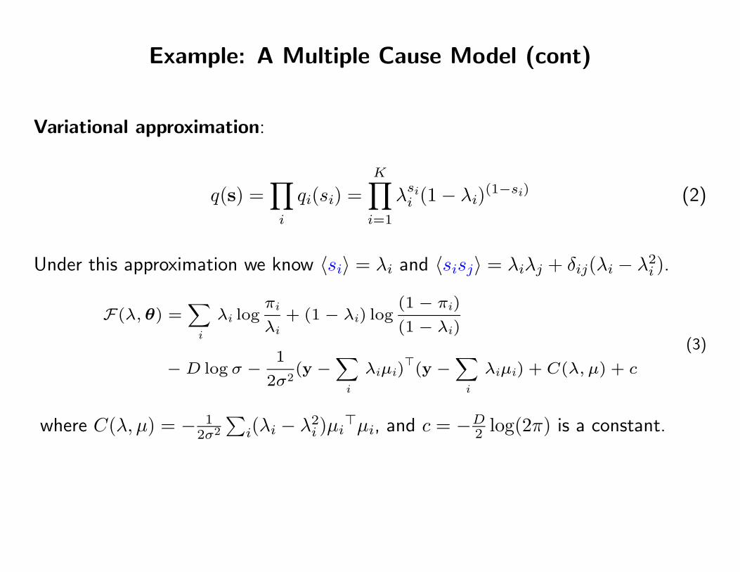
Example: A Multiple Cause Model (cont)

Variational approximation:

q(s) =∏i

qi(si) =K∏i=1

λsii (1− λi)(1−si) (2)

Under this approximation we know 〈si〉 = λi and 〈sisj〉 = λiλj + δij(λi − λ2i ).

F(λ, θ) =∑i

λi logπi

λi+ (1− λi) log

(1− πi)(1− λi)

−D log σ −1

2σ2(y −

∑i

λiµi)>

(y −∑i

λiµi) + C(λ, µ) + c

(3)

where C(λ, µ) = − 12σ2

∑i(λi − λ2

i )µi>µi, and c = −D2 log(2π) is a constant.

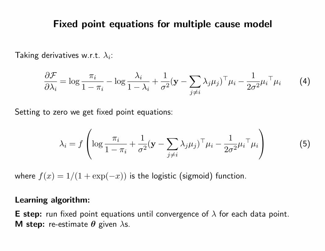
Fixed point equations for multiple cause model

Taking derivatives w.r.t. λi:

∂F∂λi

= logπi

1− πi− log

λi1− λi

+1σ2

(y −∑j 6=i

λjµj)>µi −1

2σ2µi>µi (4)

Setting to zero we get fixed point equations:

λi = f

logπi

1− πi+

1σ2

(y −∑j 6=i

λjµj)>µi −1

2σ2µi>µi

(5)

where f(x) = 1/(1 + exp(−x)) is the logistic (sigmoid) function.

Learning algorithm:

E step: run fixed point equations until convergence of λ for each data point.M step: re-estimate θ given λs.

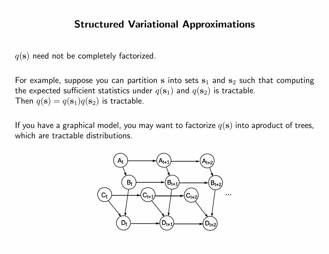
Structured Variational Approximations

q(s) need not be completely factorized.

For example, suppose you can partition s into sets s1 and s2 such that computingthe expected sufficient statistics under q(s1) and q(s2) is tractable.Then q(s) = q(s1)q(s2) is tractable.

If you have a graphical model, you may want to factorize q(s) into aproduct of trees,which are tractable distributions.

At

Dt

Ct

Bt

At+1

Dt+1

Ct+1

Bt+1

...

At+2

Dt+2

Ct+2

Bt+2

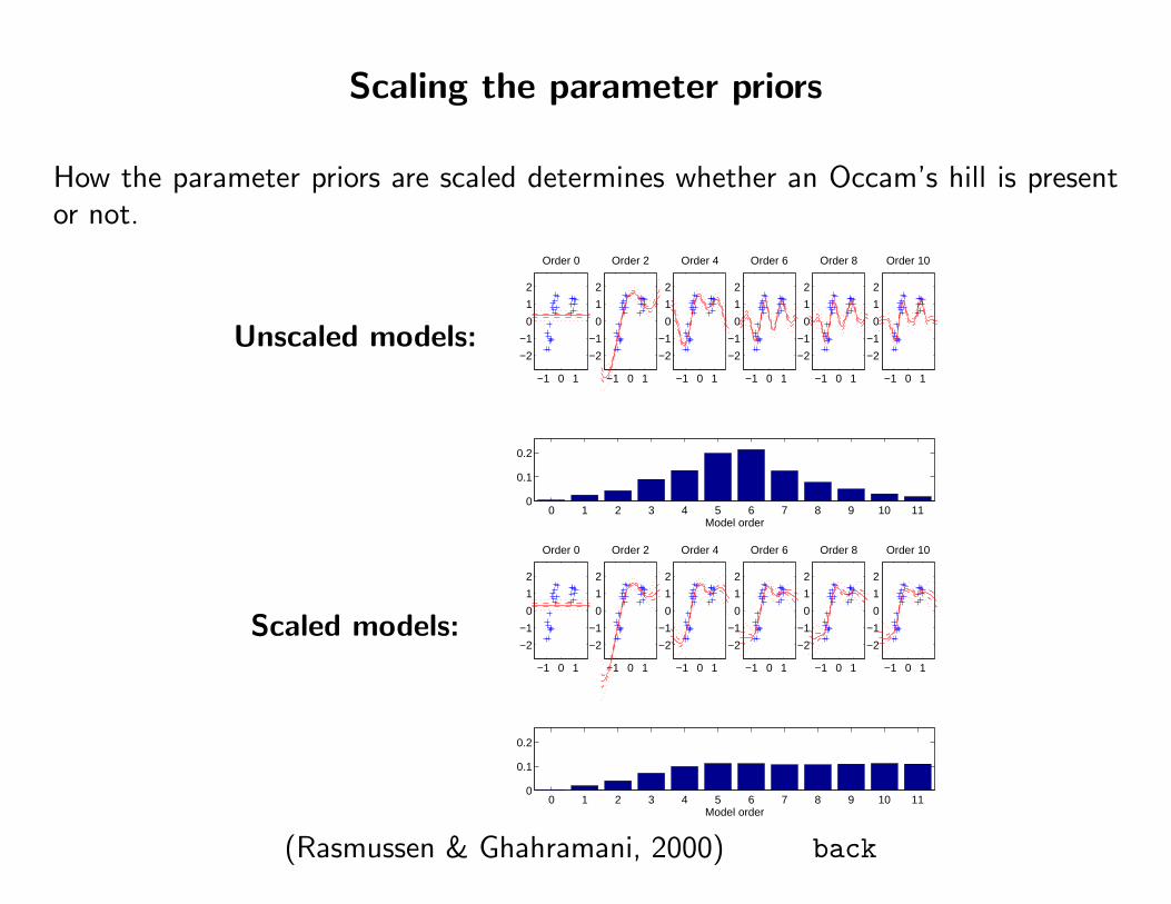
Scaling the parameter priors

How the parameter priors are scaled determines whether an Occam’s hill is presentor not.

Unscaled models:

0 1 2 3 4 5 6 7 8 9 10 110

0.1

0.2

Model order

−1 0 1

−2

−1

0

1

2

Order 0

−1 0 1

−2

−1

0

1

2

Order 2

−1 0 1

−2

−1

0

1

2

Order 4

−1 0 1

−2

−1

0

1

2

Order 6

−1 0 1

−2

−1

0

1

2

Order 8

−1 0 1

−2

−1

0

1

2

Order 10

Scaled models:

0 1 2 3 4 5 6 7 8 9 10 110

0.1

0.2

Model order

−1 0 1

−2

−1

0

1

2

Order 0

−1 0 1

−2

−1

0

1

2

Order 2

−1 0 1

−2

−1

0

1

2

Order 4

−1 0 1

−2

−1

0

1

2

Order 6

−1 0 1

−2

−1

0

1

2

Order 8

−1 0 1

−2

−1

0

1

2

Order 10

(Rasmussen & Ghahramani, 2000) back

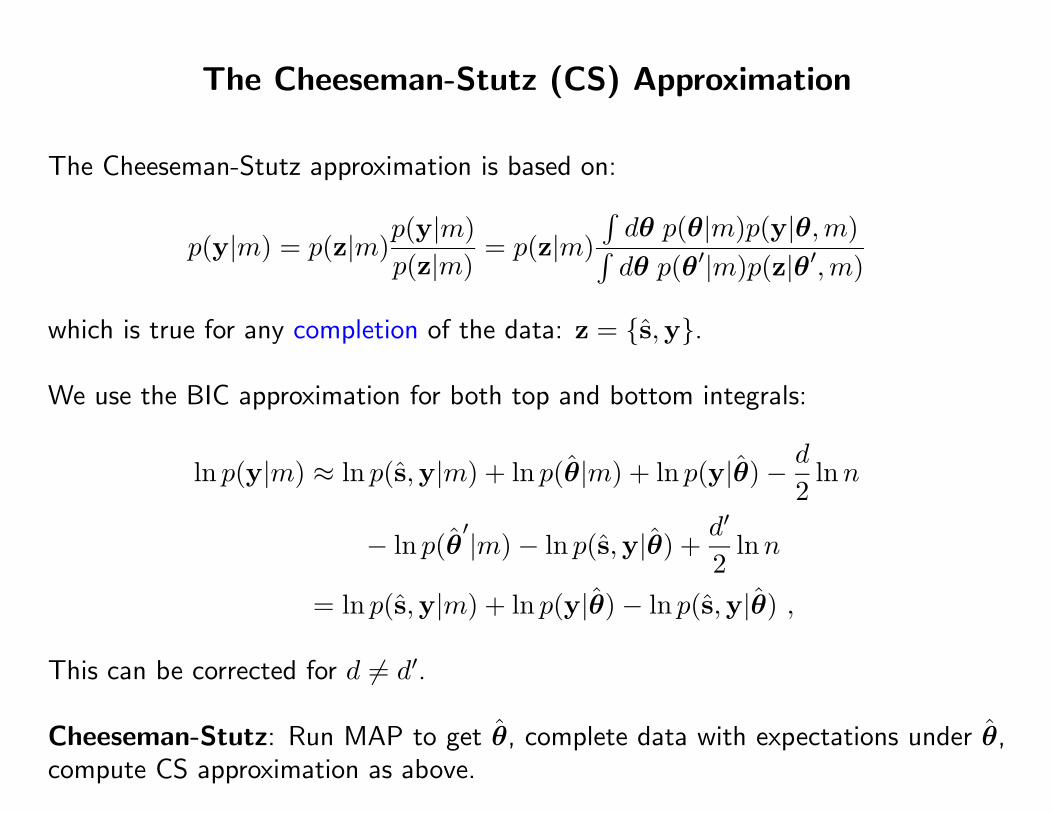
The Cheeseman-Stutz (CS) Approximation

The Cheeseman-Stutz approximation is based on:

p(y|m) = p(z|m)p(y|m)p(z|m)

= p(z|m)∫dθ p(θ|m)p(y|θ,m)∫dθ p(θ′|m)p(z|θ′,m)

which is true for any completion of the data: z = {s,y}.

We use the BIC approximation for both top and bottom integrals:

ln p(y|m) ≈ ln p(s,y|m) + ln p(θ|m) + ln p(y|θ)− d2

lnn

− ln p(θ′|m)− ln p(s,y|θ) +

d′

2lnn

= ln p(s,y|m) + ln p(y|θ)− ln p(s,y|θ) ,

This can be corrected for d 6= d′.

Cheeseman-Stutz: Run MAP to get θ, complete data with expectations under θ,compute CS approximation as above.