Lunds universitet / Kraftverksteknik / JK

Theory of turbo machinery / Turbomaskinernas teori

Chapter 1

Lunds universitet / Kraftverksteknik / JK

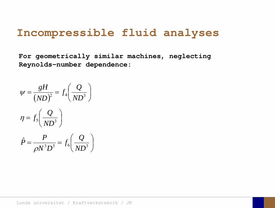
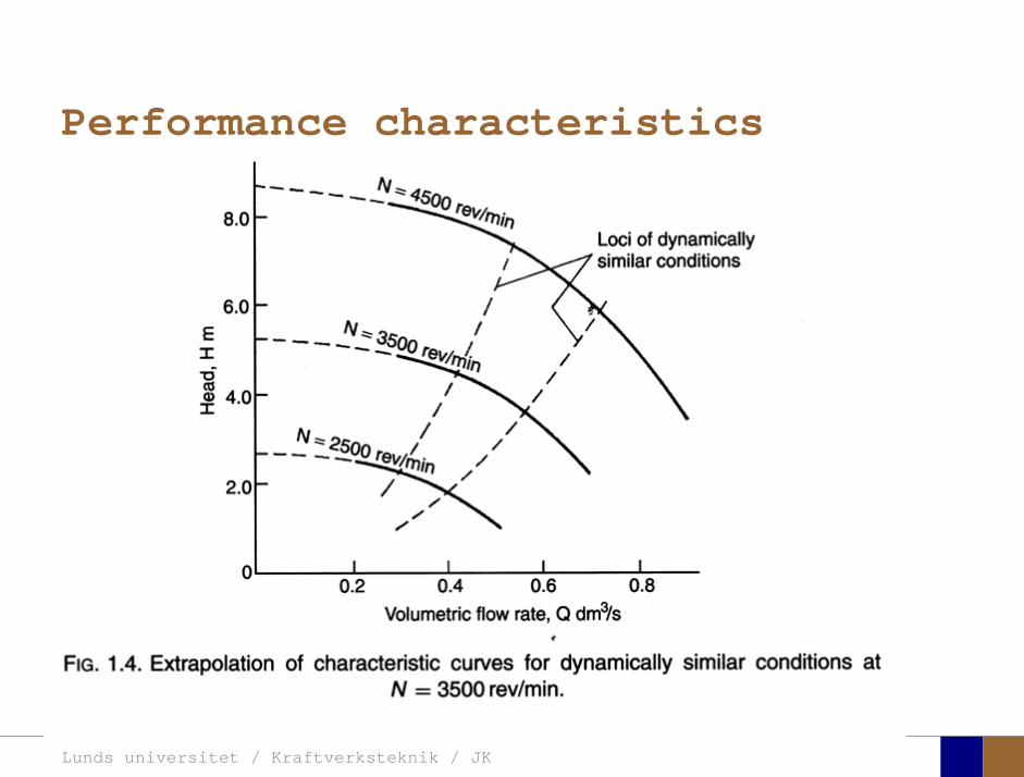
For geometrically similar machines, neglecting Reynolds-number dependence:

( ) ⎟⎠⎞

⎜⎝⎛== 342 ND

QfNDgHψ

⎟⎠⎞

⎜⎝⎛= 35 ND

Qfη

⎟⎠⎞

⎜⎝⎛== 3653

ˆNDQf

DNPP

ρ

Incompressible fluid analyses

Lunds universitet / Kraftverksteknik / JK

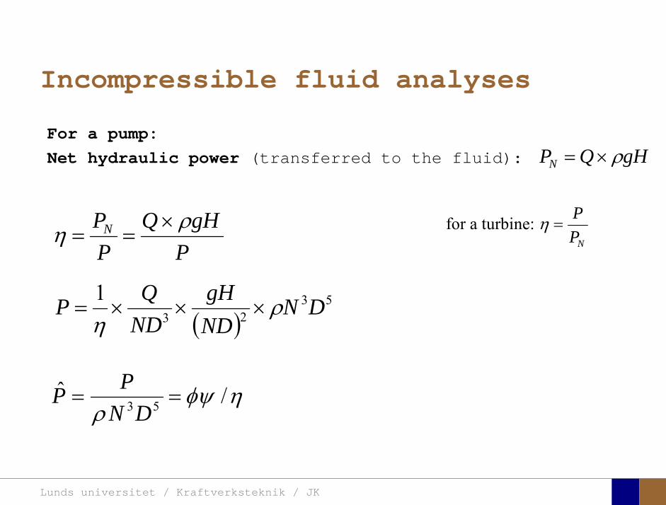
For a pump:Net hydraulic power (transferred to the fluid): gHQPN ρ×=

Incompressible fluid analyses

PgHQ

PPN ρη ×

==

( )53

23

1 DNNDgH

NDQP ρ

η×××=

3 5ˆ /PP

N Dφψ η

ρ= =

for a turbine: N

PP

η =

Lunds universitet / Kraftverksteknik / JK

Performance characteristics

Lunds universitet / Kraftverksteknik / JK

Specific speed

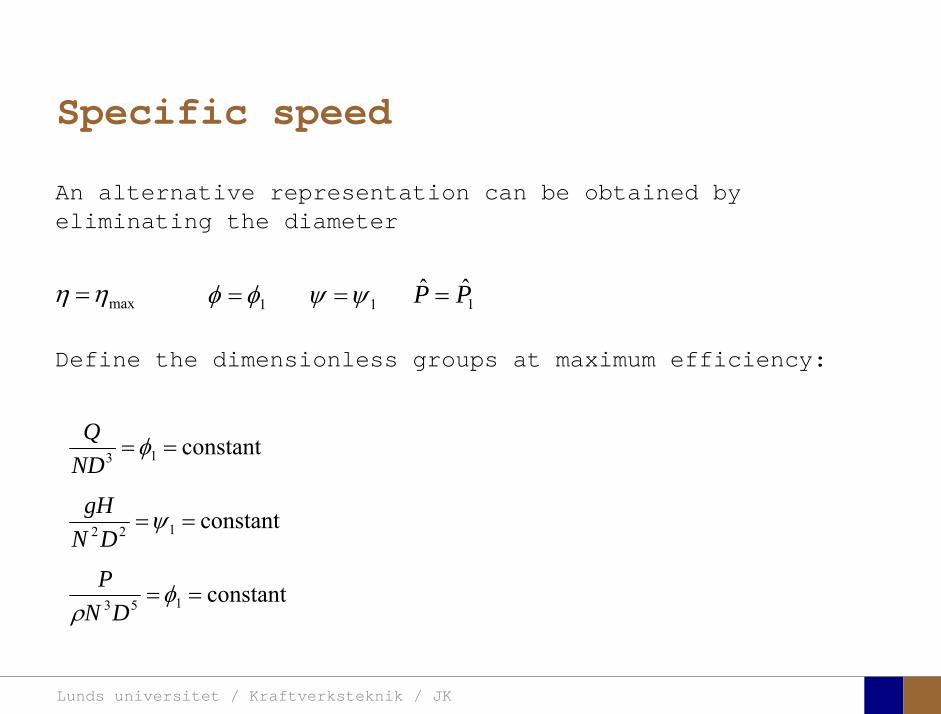
An alternative representation can be obtained by eliminating the diameter

Define the dimensionless groups at maximum efficiency:

maxηη = 1φφ = 1ψψ = 1̂ˆ PP =

constant13 ==φNDQ

constant122 ==ψDN

gH

constant153 ==φρ DN

P

Lunds universitet / Kraftverksteknik / JK

Specific speed

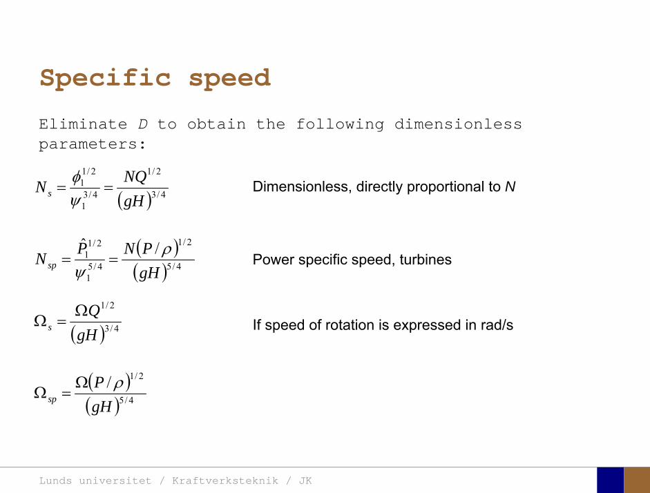
Eliminate D to obtain the following dimensionless parameters:

( ) 4/3

2/1

4/31

2/11

gHNQNs ==

ψφ

( )( ) 4/5

2/1

4/51

2/11 /ˆ

gHPNPNsp

ρψ

==

( ) 4/3

2/1

gHQ

sΩ

=Ω

( )( ) 4/5

2/1/gHP

spρΩ

=Ω

Dimensionless, directly proportional to N

Power specific speed, turbines

If speed of rotation is expressed in rad/s

Lunds universitet / Kraftverksteknik / JK

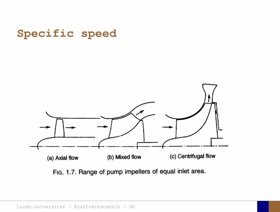
Specific speed

Lunds universitet / Kraftverksteknik / JK

Specific speed

Lunds universitet / Kraftverksteknik / JK

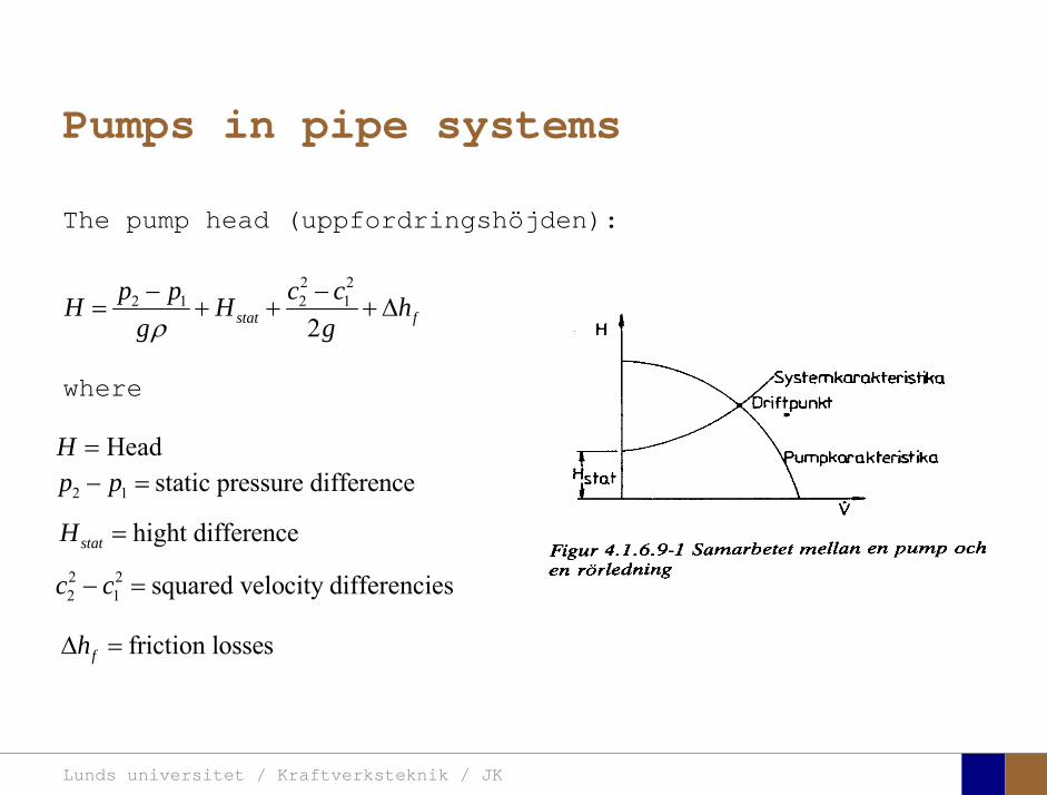
Pumps in pipe systems

The pump head (uppfordringshöjden):

2 22 1 2 1

2stat fp p c cH H h

g gρ− −

= + + + Δ

where

HeadH =

2 1 static pressure differencep p− =

hight differencestatH =

2 22 1 squared velocity differenciesc c− =

friction lossesfhΔ =

Lunds universitet / Kraftverksteknik / JK

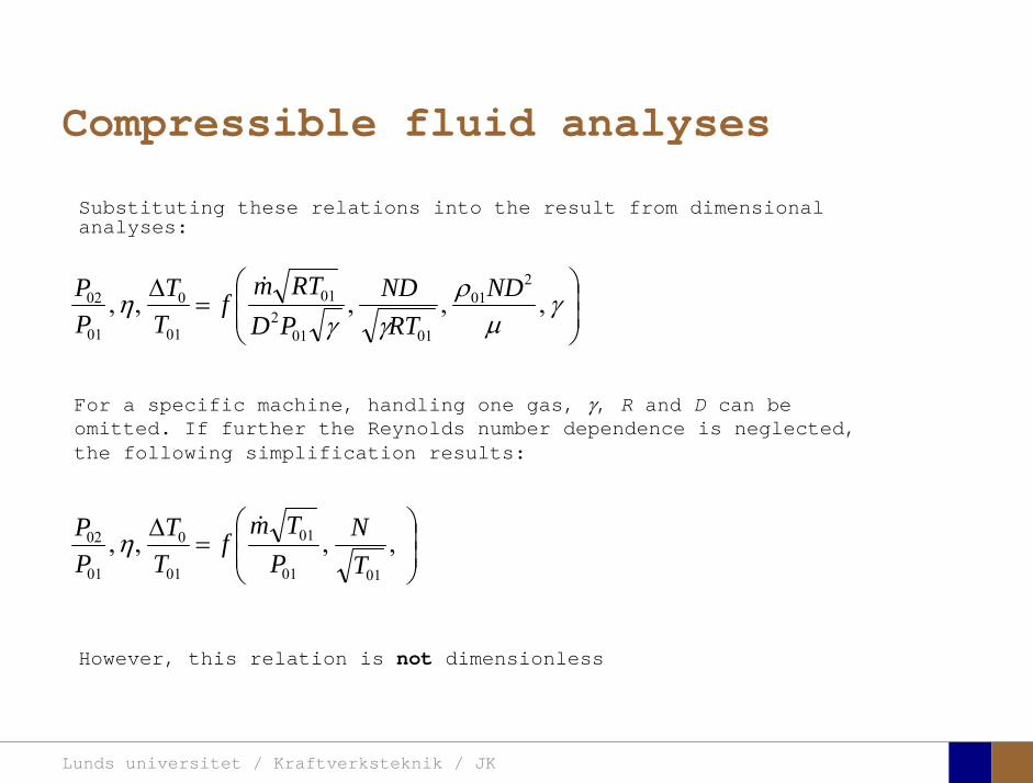
Compressible fluid analyses

Substituting these relations into the result from dimensional analyses:

For a specific machine, handling one gas, γ, R and D can be omitted. If further the Reynolds number dependence is neglected,the following simplification results:

⎟⎟⎠

⎞⎜⎜⎝

⎛=

Δ ,,,,0101

01

01

0

01

02

TN

PTm

fTT

PP η

⎟⎟⎠

⎞⎜⎜⎝

⎛=

Δ γμ

ργγ

η ,,,,,2

01

01012

01

01

0

01

02 NDRT

NDPDRTm

fTT

PP

However, this relation is not dimensionless

Lunds universitet / Kraftverksteknik / JK

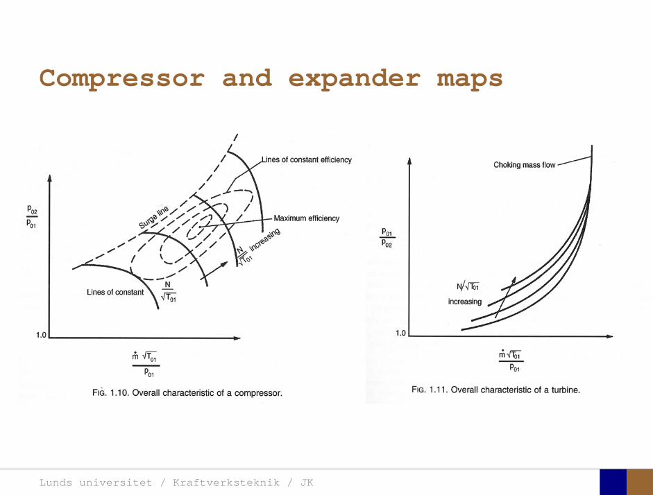
Compressor and expander maps

Lunds universitet / Kraftverksteknik / JK

Theory of turbo machinery / Turbomaskinernas teori

Chapter 2

Lunds universitet / Kraftverksteknik / JK

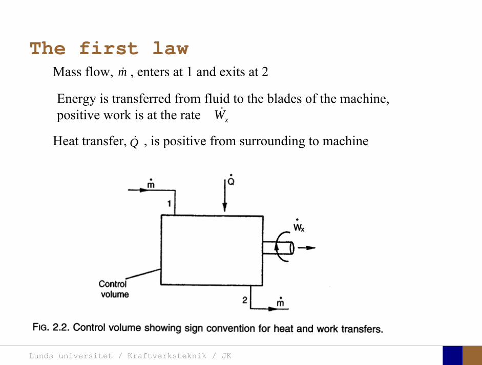
The first law

xWEnergy is transferred from fluid to the blades of the machine, positive work is at the rate

Heat transfer, , is positive from surrounding to machineQ

Mass flow, , enters at 1 and exits at 2m

Lunds universitet / Kraftverksteknik / JK

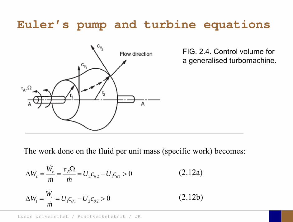
Euler’s pump and turbine equations

The work done on the fluid per unit mass (specific work) becomes:

01122 >−=Ω

==Δ θθτ cUcU

mmWW Ac

c(2.12a)

02211 >−==Δ θθ cUcUmWW t

t(2.12b)

FIG. 2.4. Control volume for a generalised turbomachine.

Lunds universitet / Kraftverksteknik / JK

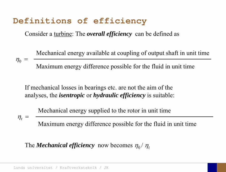
Definitions of efficiencyConsider a turbine: The overall efficiency can be defined as

Mechanical energy available at coupling of output shaft in unit time

Maximum energy difference possible for the fluid in unit time η0 =

If mechanical losses in bearings etc. are not the aim of the analyses, the isentropic or hydraulic efficiency is suitable:

Mechanical energy supplied to the rotor in unit time

Maximum energy difference possible for the fluid in unit time ηt =

The Mechanical efficiency now becomes η0 / ηt

Lunds universitet / Kraftverksteknik / JK

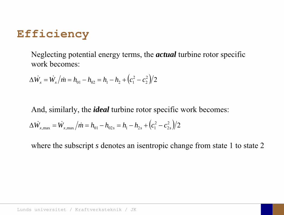
Efficiency

Neglecting potential energy terms, the actual turbine rotor specific work becomes:

And, similarly, the ideal turbine rotor specific work becomes:

where the subscript s denotes an isentropic change from state 1 to state 2

( ) 222

21210201 cchhhhmWW xx −+−=−==Δ

( ) 222

21210201max,max, sssxx cchhhhmWW −+−=−==Δ

Lunds universitet / Kraftverksteknik / JK

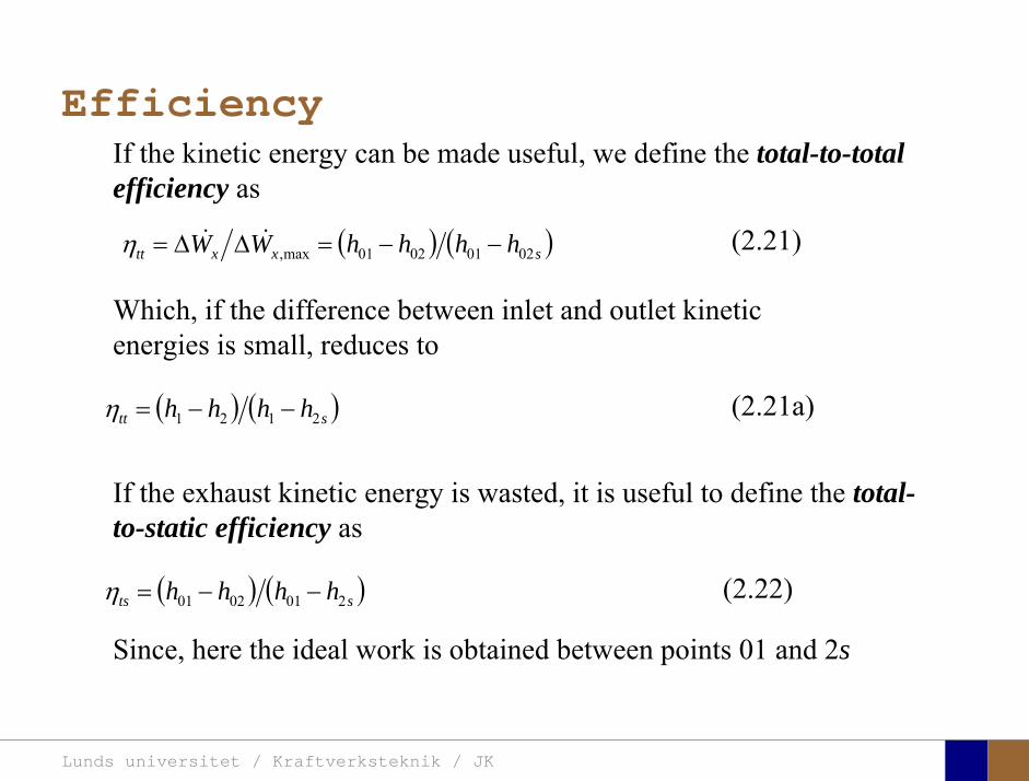
EfficiencyIf the kinetic energy can be made useful, we define the total-to-total efficiency as

Which, if the difference between inlet and outlet kinetic energies is small, reduces to

( ) ( )sxxtt hhhhWW 02010201max, −−=ΔΔ=η

( ) ( )stt hhhh 2121 −−=η

(2.21)

(2.21a)

If the exhaust kinetic energy is wasted, it is useful to define the total-to-static efficiency as

( ) ( )sts hhhh 2010201 −−=η (2.22)

Since, here the ideal work is obtained between points 01 and 2s

Lunds universitet / Kraftverksteknik / JK

Efficiency

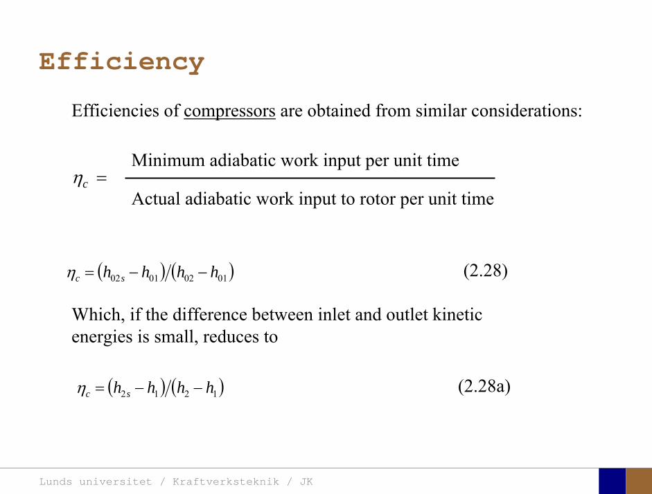
Efficiencies of compressors are obtained from similar considerations:

( ) ( )01020102 hhhh sc −−=η (2.28)

(2.28a)

Minimum adiabatic work input per unit time

Actual adiabatic work input to rotor per unit timeηc =

Which, if the difference between inlet and outlet kinetic energies is small, reduces to

( ) ( )1212 hhhh sc −−=η

Lunds universitet / Kraftverksteknik / JK

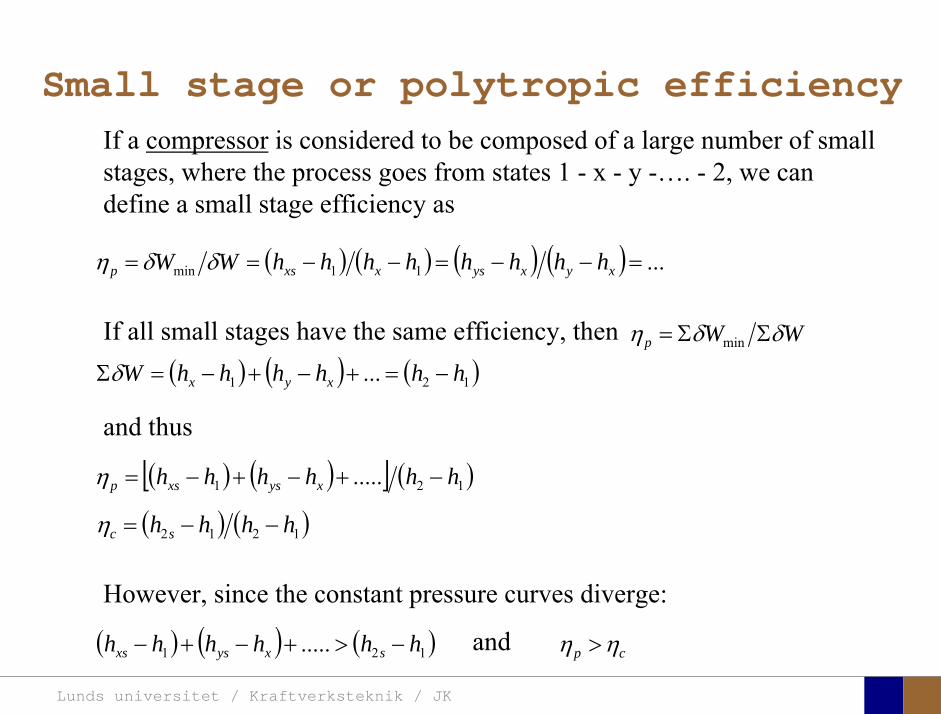
Small stage or polytropic efficiencyIf a compressor is considered to be composed of a large number of small stages, where the process goes from states 1 - x - y -…. - 2, we can define a small stage efficiency as

( ) ( ) ( ) ( ) ...11min =−−=−−== xyxysxxsp hhhhhhhhWW δδη

If all small stages have the same efficiency, then

However, since the constant pressure curves diverge:

WWp δδη ΣΣ= min

( ) ( ) ( )121 ... hhhhhhW xyx −=+−+−=Σδ

and thus

( ) ( )[ ] ( )121 ..... hhhhhh xysxsp −+−+−=η

( ) ( )1212 hhhh sc −−=η

( ) ( ) ( )121 ..... hhhhhh sxysxs −>+−+− and cp ηη >

Lunds universitet / Kraftverksteknik / JK

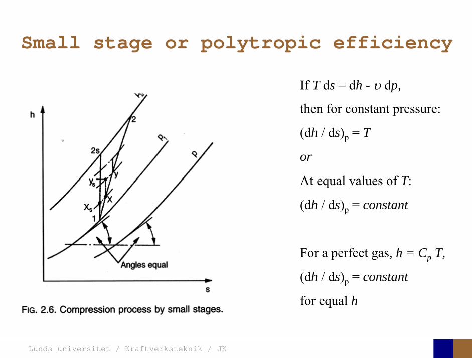
If T ds = dh - υ dp,

then for constant pressure:

(dh / ds)p = T

or

At equal values of T:

(dh / ds)p = constant

For a perfect gas, h = Cp T,

(dh / ds)p = constant

for equal h

Small stage or polytropic efficiency

Lunds universitet / Kraftverksteknik / JK

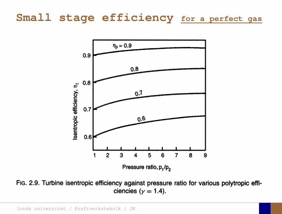
Small stage efficiency for a perfect gas

Lunds universitet / Kraftverksteknik / JK

Small stage efficiency for a perfect gas

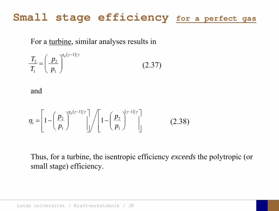
For a turbine, similar analyses results in

( ) ( )

⎥⎥⎦

⎤

⎢⎢⎣

⎡⎟⎟⎠

⎞⎜⎜⎝

⎛−

⎥⎥⎦

⎤

⎢⎢⎣

⎡⎟⎟⎠

⎞⎜⎜⎝

⎛−=

−− γγγγη

η1

1

2

1

1

2 11pp

pp p

t (2.38)

and

( ) γγη 1

1

2

1

2

−

⎟⎟⎠

⎞⎜⎜⎝

⎛=

p

pp

TT

(2.37)

Thus, for a turbine, the isentropic efficiency exceeds the polytropic (or small stage) efficiency.

Lunds universitet / Kraftverksteknik / JK

Small stage efficiency for a perfect gas

Lunds universitet / Kraftverksteknik / JK

Theory of turbo machinery / Turbomaskinernas teori

Chapter 3

Lunds universitet / Kraftverksteknik / JK

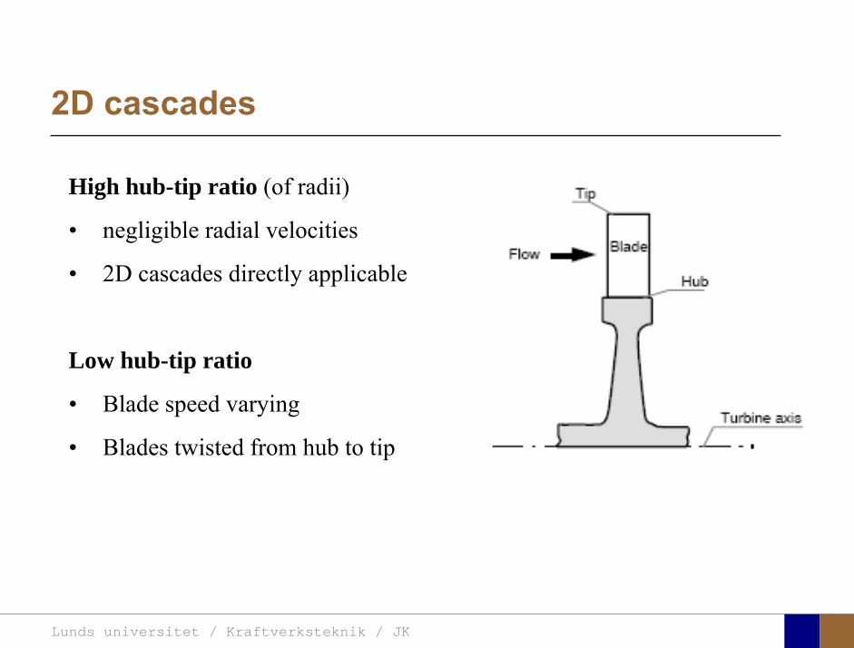
2D cascades

High hub-tip ratio (of radii)

• negligible radial velocities

• 2D cascades directly applicable

Low hub-tip ratio

• Blade speed varying

• Blades twisted from hub to tip

Lunds universitet / Kraftverksteknik / JK

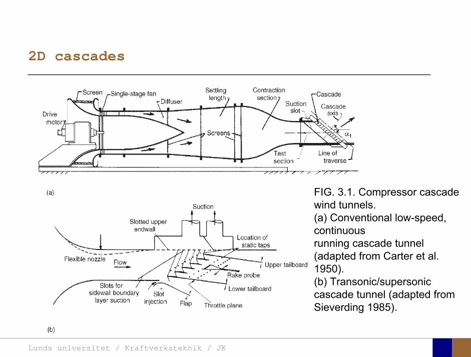
2D cascades

FIG. 3.1. Compressor cascadewind tunnels. (a) Conventional low-speed, continuousrunning cascade tunnel (adapted from Carter et al. 1950).(b) Transonic/supersoniccascade tunnel (adapted from Sieverding 1985).

Lunds universitet / Kraftverksteknik / JK

2D cascades

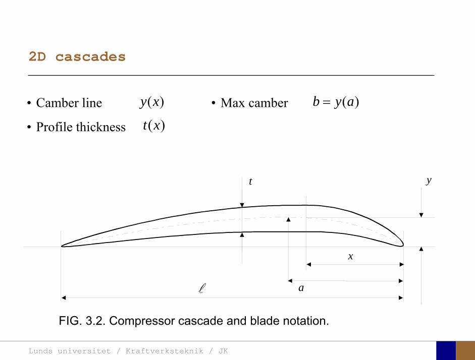
FIG. 3.2. Compressor cascade and blade notation.

( )y x• Camber line

• Profile thickness ( )t x

a

x

t y

( )b y a=• Max camber

Lunds universitet / Kraftverksteknik / JK

2D cascades

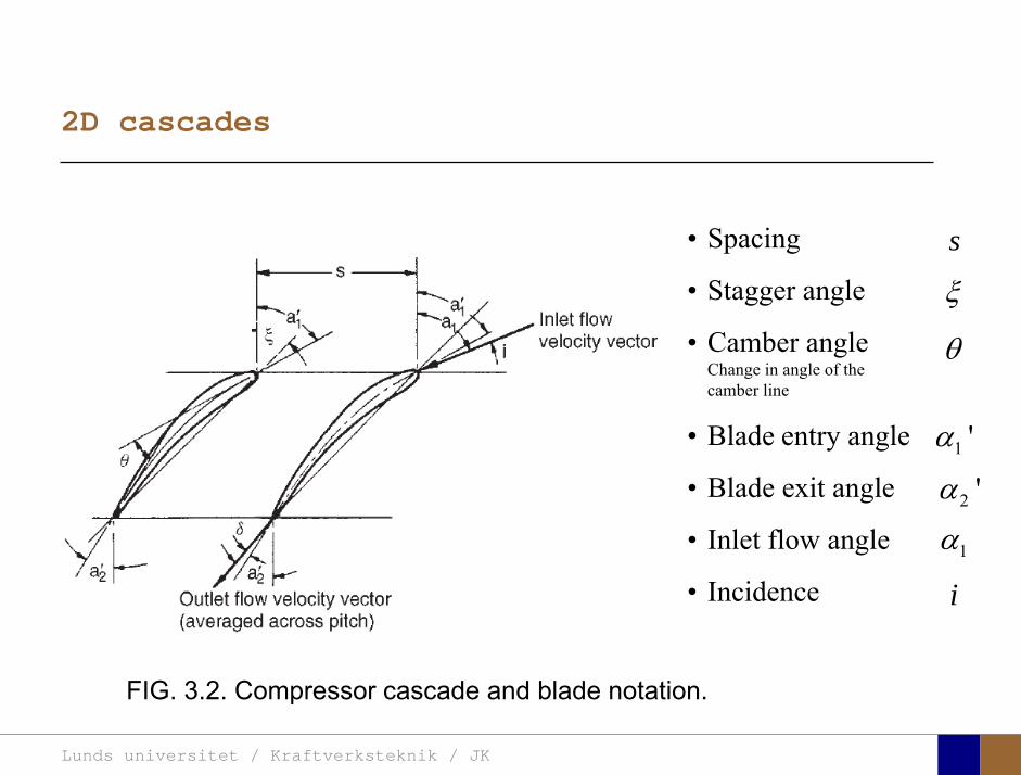
FIG. 3.2. Compressor cascade and blade notation.

s• Spacing

• Stagger angle

• Camber angleChange in angle of the camber line

• Blade entry angle

• Blade exit angle

• Inlet flow angle

• Incidence

ξ

θ

1 'α

2 'α

1α

i

Lunds universitet / Kraftverksteknik / JK

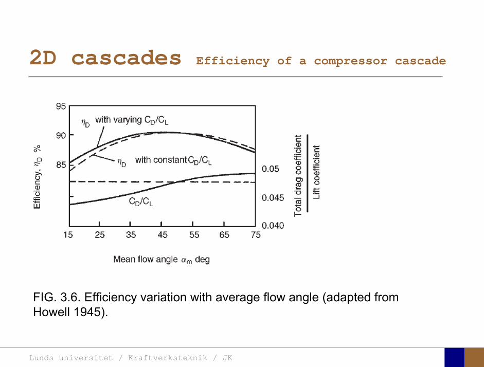
2D cascades Efficiency of a compressor cascade

FIG. 3.6. Efficiency variation with average flow angle (adapted from Howell 1945).

Lunds universitet / Kraftverksteknik / JK

2D cascades Fluid deviation

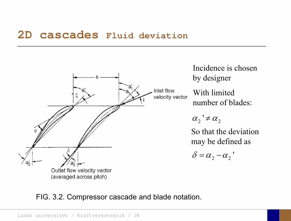
FIG. 3.2. Compressor cascade and blade notation.

Incidence is chosen by designer

With limited number of blades:

2 2'α α≠So that the deviation may be defined as

2 2 'δ α α= −

Lunds universitet / Kraftverksteknik / JK

2D cascades Generalizing experimental results

2 2 'δ α α= −

Deviation by Howell: Nominal deviation a function of camber and space chord ratio:

( )* nm s lδ θ=

( ) *2

0.50.23 2 500

nm a l a=

= +

with the following constants for compressor cascades

Lunds universitet / Kraftverksteknik / JK

2D cascades Optimum space chord ratio of turbineblades (Zweifel)

FIG. 3.27. Pressure distribution around a turbine cascade blade (after Zweifel 1945).

Lunds universitet / Kraftverksteknik / JK

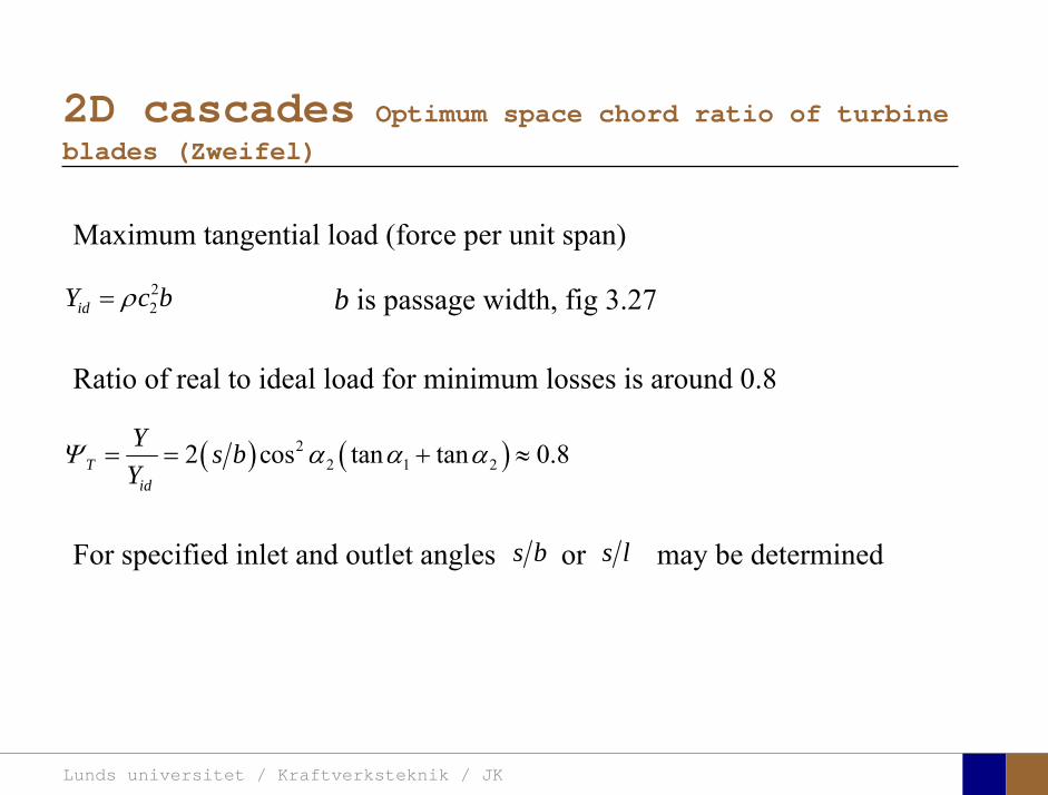
2D cascades Optimum space chord ratio of turbineblades (Zweifel)

22idY c bρ=

Maximum tangential load (force per unit span)

b is passage width, fig 3.27

Ratio of real to ideal load for minimum losses is around 0.8

( ) ( )22 1 22 cos tan tan 0.8T

id

Y s bY

Ψ α α α= = + ≈

For specified inlet and outlet angles s b or s l may be determined

Lunds universitet / Kraftverksteknik / JK

Theory of turbo machinery / Turbomaskinernas teori

Chapter 4

Lunds universitet / Kraftverksteknik / JK

Axial-flow Turbines: 2-D theory

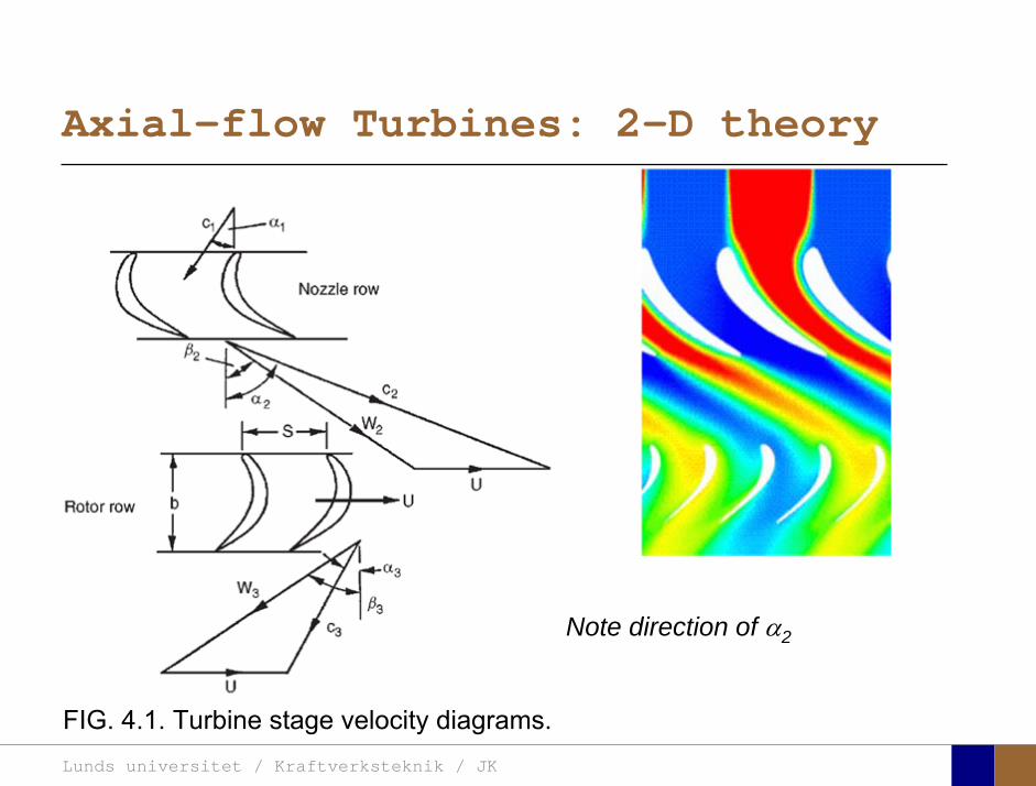
FIG. 4.1. Turbine stage velocity diagrams.

Note direction of α2

Lunds universitet / Kraftverksteknik / JK

Axial-flow Turbines: 2-D theory

Assumptions:

• Hub to tip ratio high (close to 1)

• Negligible radial velocities

• No changes in circumferential direction (wakes and nonuniformoutlet velocity distribution neglected)

Lunds universitet / Kraftverksteknik / JK

Axial-flow Turbines: 2-D theory

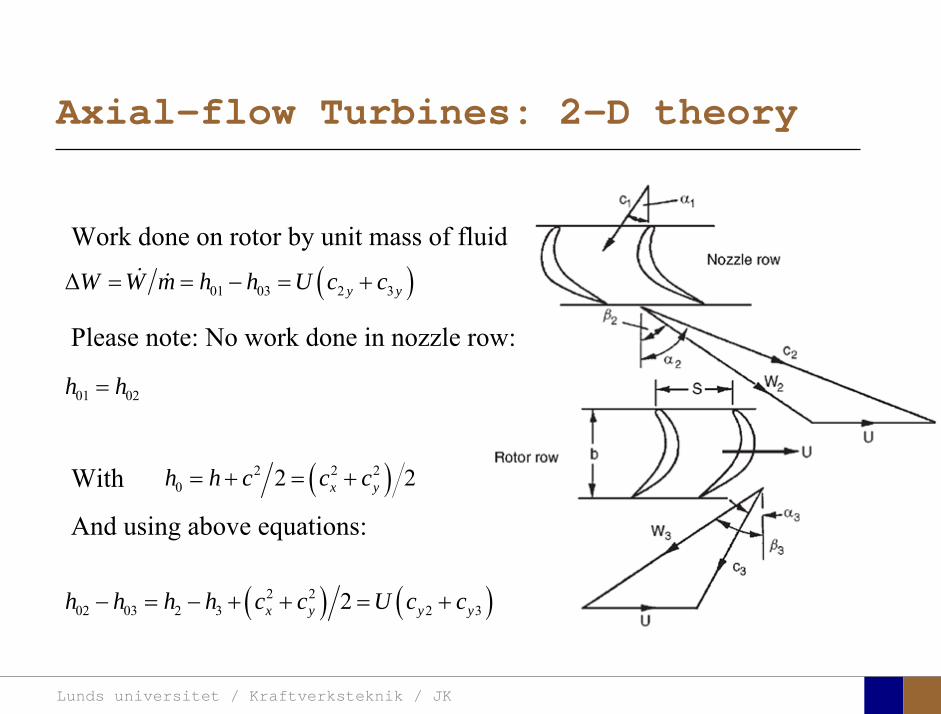
( )01 03 2 3Δ y yW W m h h U c c= = − = +

01 02h h=

Please note: No work done in nozzle row:

With

And using above equations:

( )2 2 20 2 2x yh h c c c= + = +

Work done on rotor by unit mass of fluid

( ) ( )2 202 03 2 3 2 32x y y yh h h h c c U c c− = − + + = +

Lunds universitet / Kraftverksteknik / JK

Axial-flow Turbines: 2-D theory

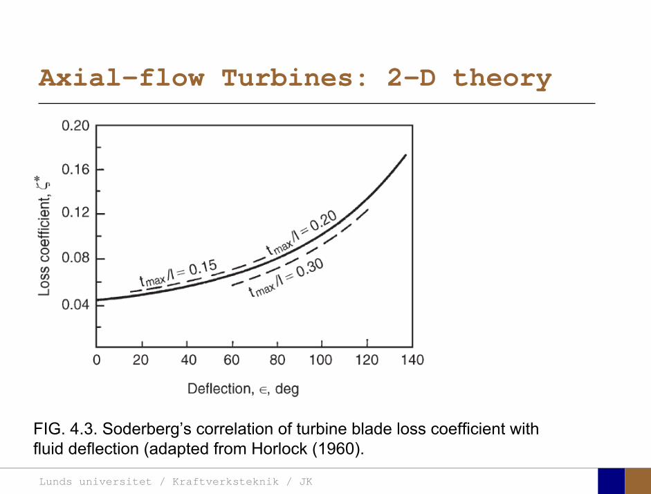
FIG. 4.3. Soderberg’s correlation of turbine blade loss coefficient with fluid deflection (adapted from Horlock (1960).

Lunds universitet / Kraftverksteknik / JK

Axial-flow Turbines: 2-D theory

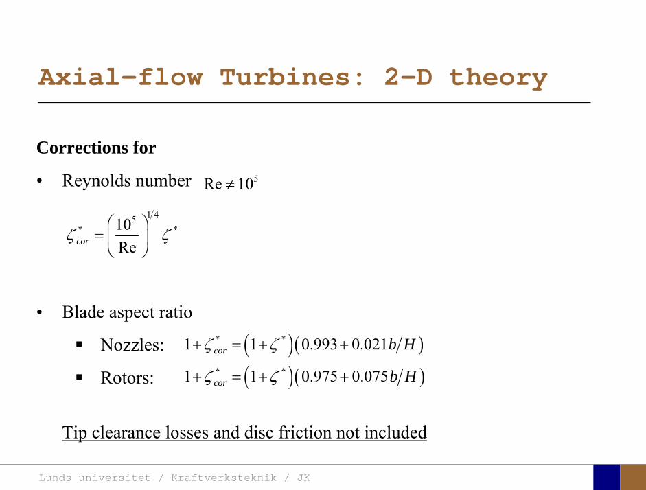
Corrections for

• Reynolds number

• Blade aspect ratio

Nozzles:

Rotors:

Tip clearance losses and disc friction not included

5Re 10≠

1 45* *10

Recorζ ζ⎛ ⎞

= ⎜ ⎟⎝ ⎠

( )( )* *1 1 0.993 0.021cor b Hζ ζ+ = + +

( )( )* *1 1 0.975 0.075cor b Hζ ζ+ = + +

Lunds universitet / Kraftverksteknik / JK

Axial-flow Turbines: 2-D theory

Design considerations

• Rotor angular velocity (stresses, grid phasing)

• Weight (aircraft)

• Outside diameter (aircraft)

• Efficiency (almost always)

• ………

Lunds universitet / Kraftverksteknik / JK

Axial-flow Turbines: 2-D theory

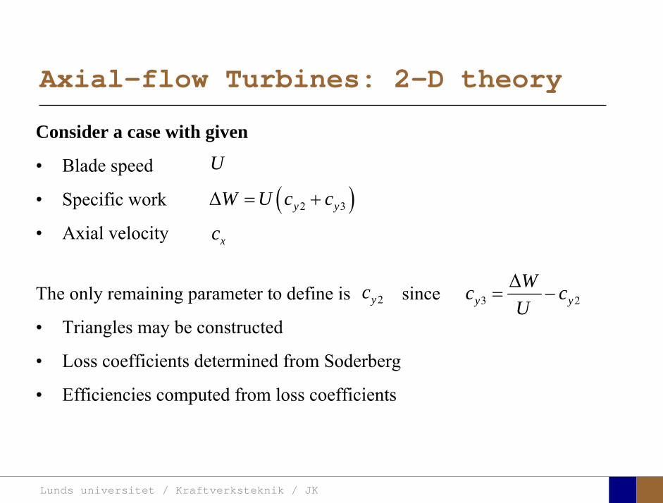
Consider a case with given

• Blade speed

• Specific work

• Axial velocity

U

( )2 3Δ y yW U c c= +

xc

The only remaining parameter to define is since

• Triangles may be constructed

• Loss coefficients determined from Soderberg

• Efficiencies computed from loss coefficients

2yc 3 2Δ

y yWc c

U= −

Lunds universitet / Kraftverksteknik / JK

Axial-flow Turbines: 2-D theory

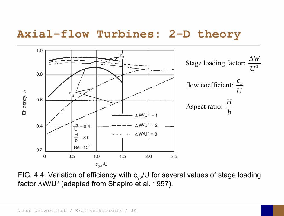
FIG. 4.4. Variation of efficiency with cy2/U for several values of stage loadingfactor ΔW/U2 (adapted from Shapiro et al. 1957).

2

ΔStage loading factor: WU

flow coefficient: xcU

Aspect ratio: Hb

Lunds universitet / Kraftverksteknik / JK

Axial-flow Turbines: 2-D theory

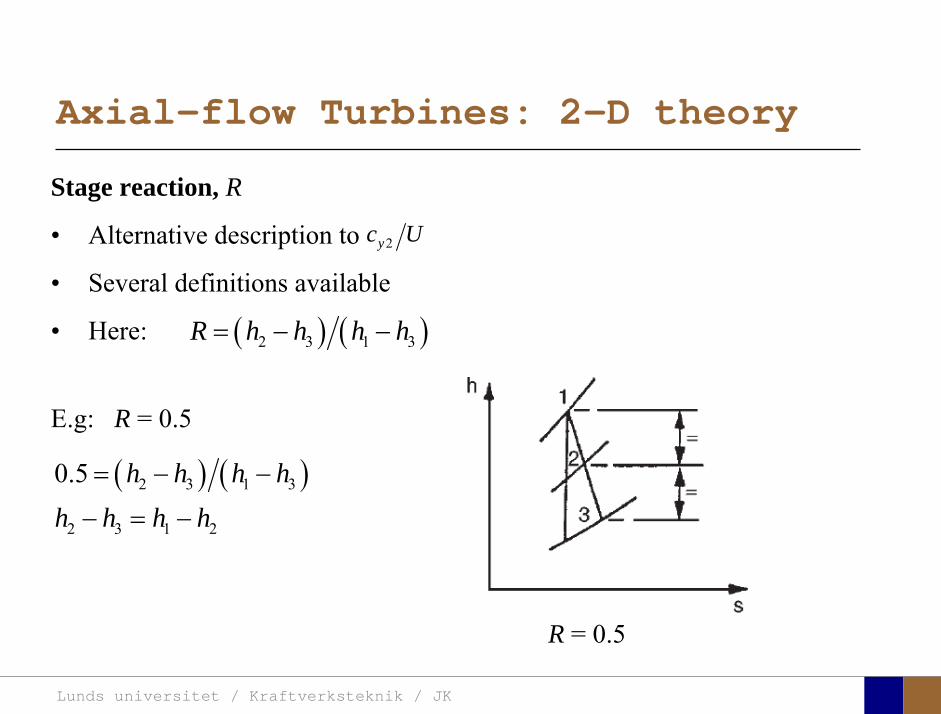
Stage reaction, R

• Alternative description to

• Several definitions available

• Here:

2yc U

( ) ( )2 3 1 3R h h h h= − −

E.g: R = 0.5

( ) ( )2 3 1 3

2 3 1 2

0.5 h h h hh h h h

= − −

− = −

R = 0.5

Lunds universitet / Kraftverksteknik / JK

Axial-flow Turbines: 2-D theory

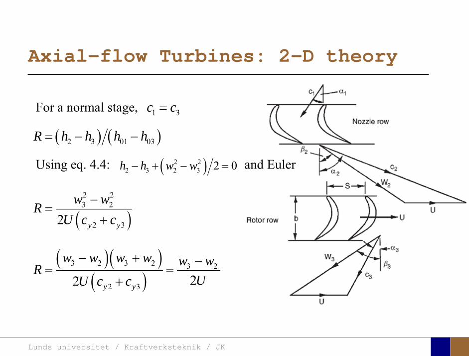
( ) ( )2 3 01 03R h h h h= − −

1 3c cFor a normal stage, =

Using eq. 4.4: and Euler( )2 22 3 2 3 2 0h h w w− + − =

( )2 23 2

2 32 y y

w wRU c c

−=

+

( )( )( )

3 2 3 2 3 2

2 3 22 y y

w w w w w wRUU c c

− + −= =

+

Lunds universitet / Kraftverksteknik / JK

Axial-flow Turbines: 2-D theory

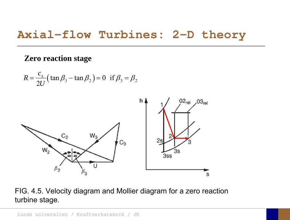
FIG. 4.5. Velocity diagram and Mollier diagram for a zero reactionturbine stage.

( )3 2 3 2tan tan 0 if 2

xcRU

β β β β= − = =

Zero reaction stage

Lunds universitet / Kraftverksteknik / JK

Axial-flow Turbines: 2-D theory

FIG. 4.7. Velocity diagram and Mollier diagram for a 50% reactionturbine stage.

( )3 2 3 21 tan tan 0.5 if 2 2

xcRU

β α β α= + − = =

50% reaction stage

Lunds universitet / Kraftverksteknik / JK

Axial-flow Turbines: 2-D theory

Turbine blade cooling.

Why is the efficiency of the gas turbine comparable to that of a Rankine cycle?

(given that we do have to pay a considerable amount of energy to the compressor, whereas compression of water in the Rankine cycle is cheap)

Lunds universitet / Kraftverksteknik / JK

Theory of turbo machinery / Turbomaskinernas teori

Dixon, chapter 7

Centrifugal Pumps, Fans and Compressors

Lunds universitet / Kraftverksteknik / JK

Centrifugal Pumps, Fans and Compressors

( ) 4/3

2/1

4/31

2/11

gHNQN s ==

ψφ

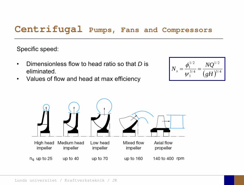
Specific speed:

• Dimensionless flow to head ratio so that D is eliminated.

• Values of flow and head at max efficiency

Lunds universitet / Kraftverksteknik / JK

Centrifugal Pumps, Fans and Compressors

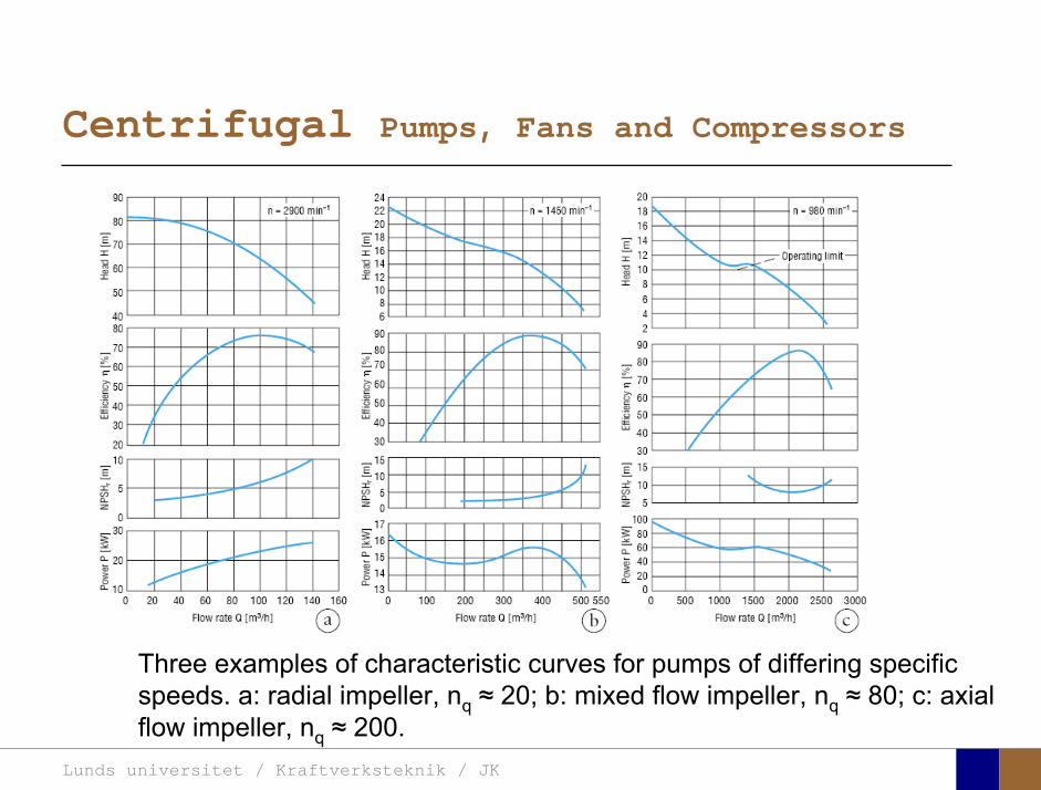
Three examples of characteristic curves for pumps of differing specificspeeds. a: radial impeller, nq ≈ 20; b: mixed flow impeller, nq ≈ 80; c: axial flow impeller, nq ≈ 200.

Lunds universitet / Kraftverksteknik / JK

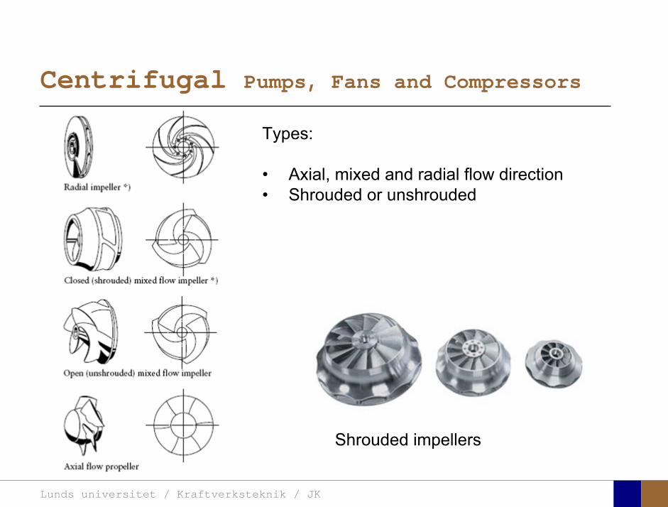
Centrifugal Pumps, Fans and Compressors

Types:

• Axial, mixed and radial flow direction• Shrouded or unshrouded

Shrouded impellers

Lunds universitet / Kraftverksteknik / JK

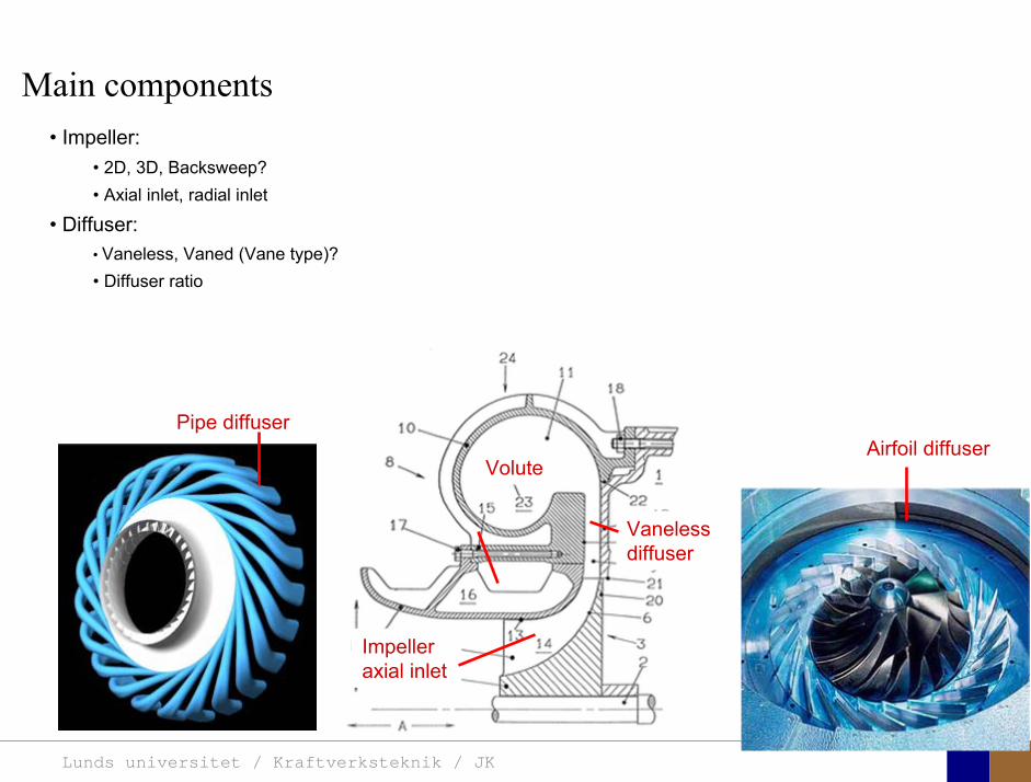
• Impeller:• 2D, 3D, Backsweep?• Axial inlet, radial inlet

• Diffuser:• Vaneless, Vaned (Vane type)? • Diffuser ratio

Volute

Vanelessdiffuser

Impeller axial inlet

Main components

Pipe diffuserAirfoil diffuser

Lunds universitet / Kraftverksteknik / JK

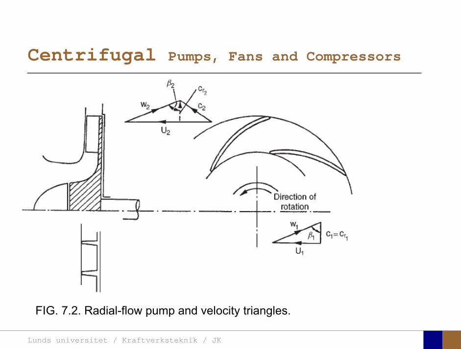
Centrifugal Pumps, Fans and Compressors

FIG. 7.2. Radial-flow pump and velocity triangles.

Lunds universitet / Kraftverksteknik / JK

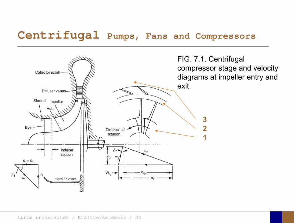
Centrifugal Pumps, Fans and Compressors

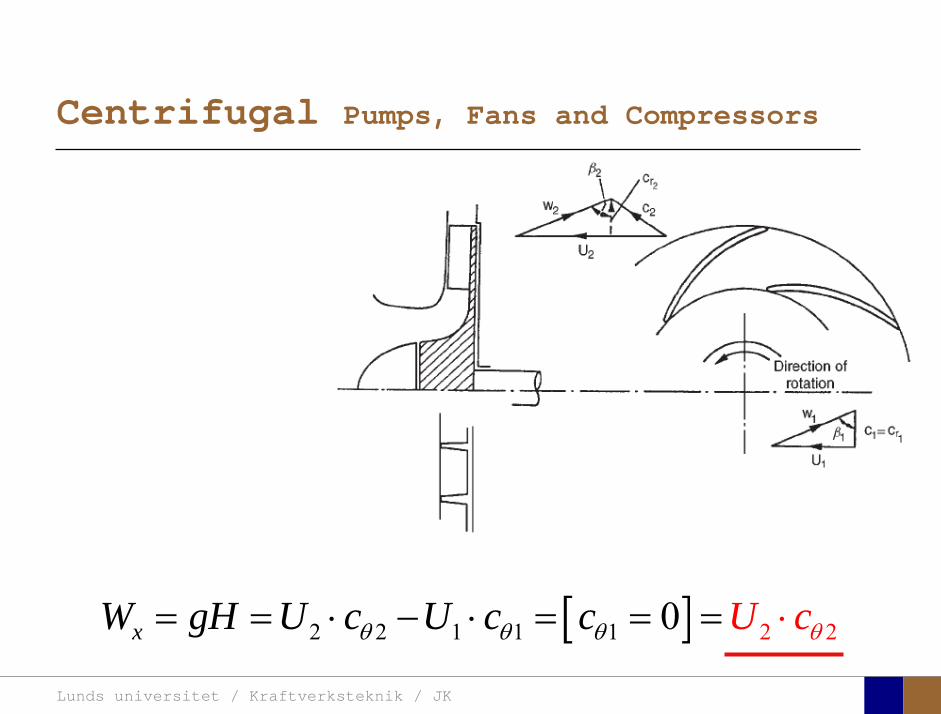
FIG. 7.1. Centrifugal compressor stage and velocitydiagrams at impeller entry and exit.

321

Lunds universitet / Kraftverksteknik / JK

Centrifugal Pumps, Fans and Compressors

[ ]2 1 21 1 22 0xW gH U c U c c U cθ θθ θ= = ⋅ ⋅ = ⋅− = =

Lunds universitet / Kraftverksteknik / JK

Centrifugal Pumps, Fans and Compressors

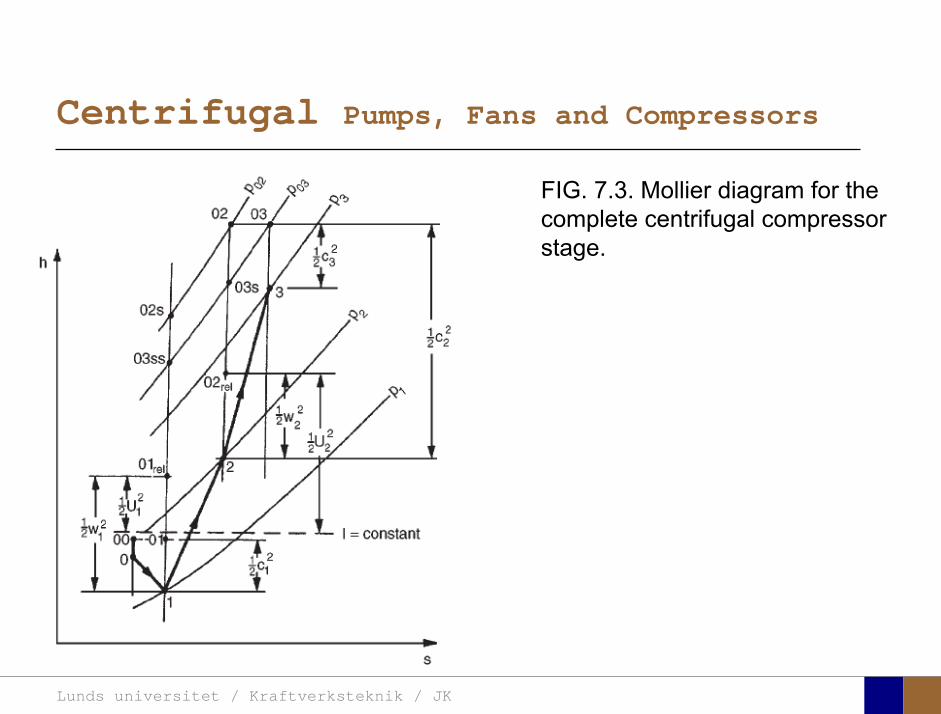
FIG. 7.3. Mollier diagram for the complete centrifugal compressorstage.

Lunds universitet / Kraftverksteknik / JK

Centrifugal Pumps, Fans and Compressors

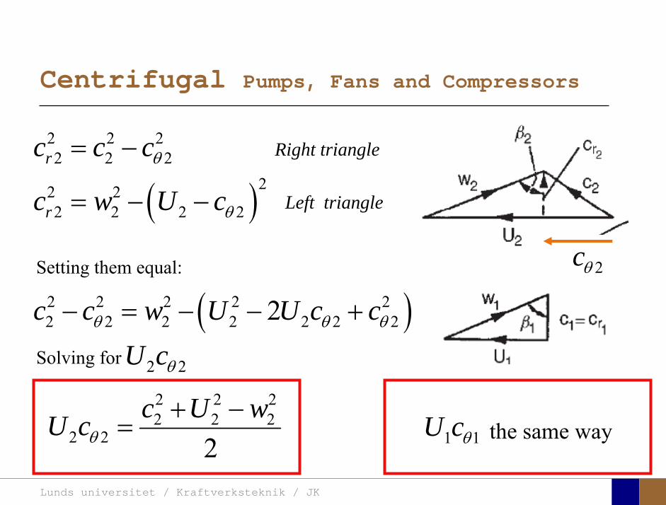
2cθ

2 2 22 2 2rc c cθ= −

( )22 22 2 2 2rc w U cθ= − −

( )2 2 2 2 22 2 2 2 2 2 22c c w U U c cθ θ θ− = − − +

Solving for 2 2U c

Setting them equal:

θ

2 2 22 2 2

2 2 2c U wU cθ+ −

= the same way1 1U cθ

Right triangle

Left triangle

Lunds universitet / Kraftverksteknik / JK

Centrifugal Pumps, Fans and Compressors

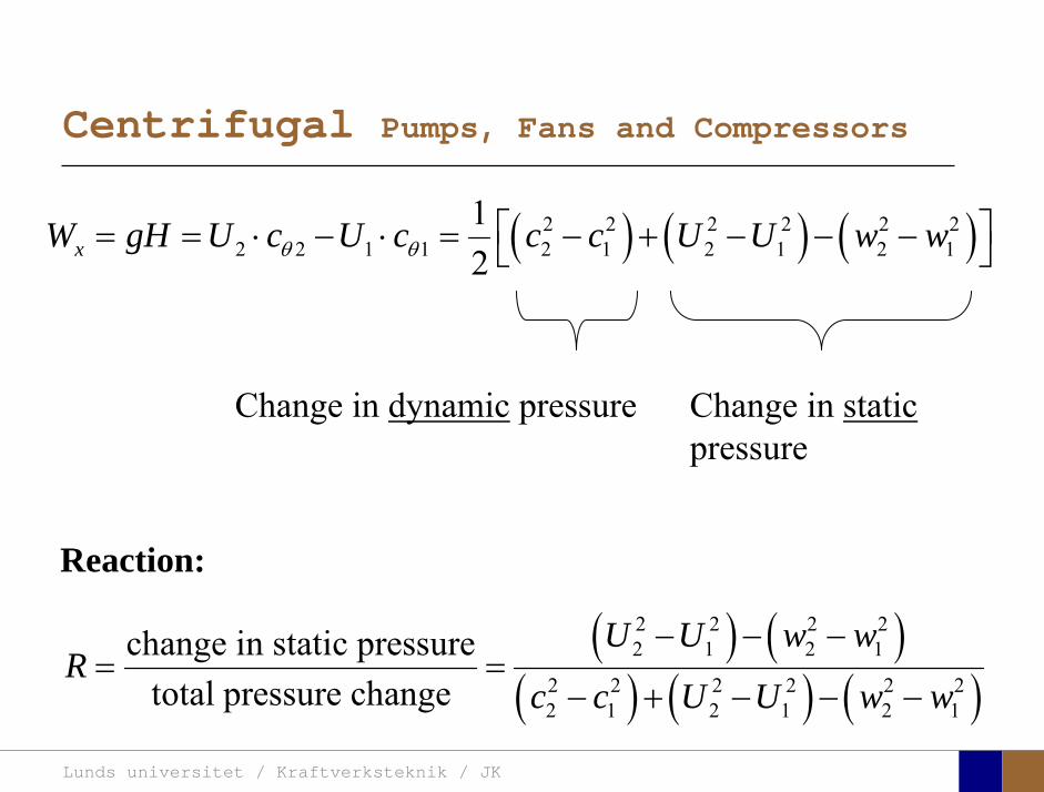
( ) ( ) ( )2 2 2 2 2 22 2 1 1 2 1 2 1 2 1

12xW gH U c U c c c U U w wθ θ⎡ ⎤= = ⋅ − ⋅ = − + − − −⎣ ⎦

Change in dynamic pressure Change in staticpressure

( ) ( )( ) ( ) ( )

2 2 2 22 1 2 1

2 2 2 2 2 22 1 2 1 2 1

change in static pressuretotal pressure change

U U w wR

c c U U w w

− − −= =

− + − − −

Reaction:

Lunds universitet / Kraftverksteknik / JK

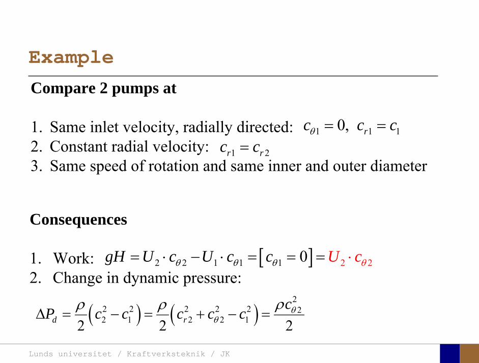
Example

1 2r rc c=

[ ] 22 2 1 1 1 20 UgH U c U c ccθ θ θ θ= ⋅ − ⋅ ⋅= = =

Compare 2 pumps at

1. Same inlet velocity, radially directed:2. Constant radial velocity: 3. Same speed of rotation and same inner and outer diameter

1 1 10, rc c cθ = =

Consequences

1. Work:2. Change in dynamic pressure:

( ) ( )2

2 2 2 2 2 22 1 2 2 12 2 2d r

cP c c c c c θθ

ρρ ρΔ = − = + − =

Lunds universitet / Kraftverksteknik / JK

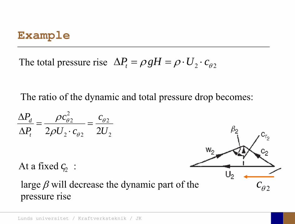
Example

2 2tP gH U cθρ ρΔ = = ⋅ ⋅The total pressure rise

22 2

2 2 22 2d

t

P c cP U c U

θ θ

θ

ρρ

Δ= =

Δ ⋅

The ratio of the dynamic and total pressure drop becomes:

2cθ2rcAt a fixed :

large β will decrease the dynamic part of the pressure rise

Lunds universitet / Kraftverksteknik / JK

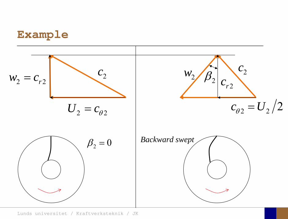
Example

2 2U cθ=

2c2rc

2 2 2c Uθ =

2c2w

2 2rw c= 2β

Backward swept2 0β =

Lunds universitet / Kraftverksteknik / JK

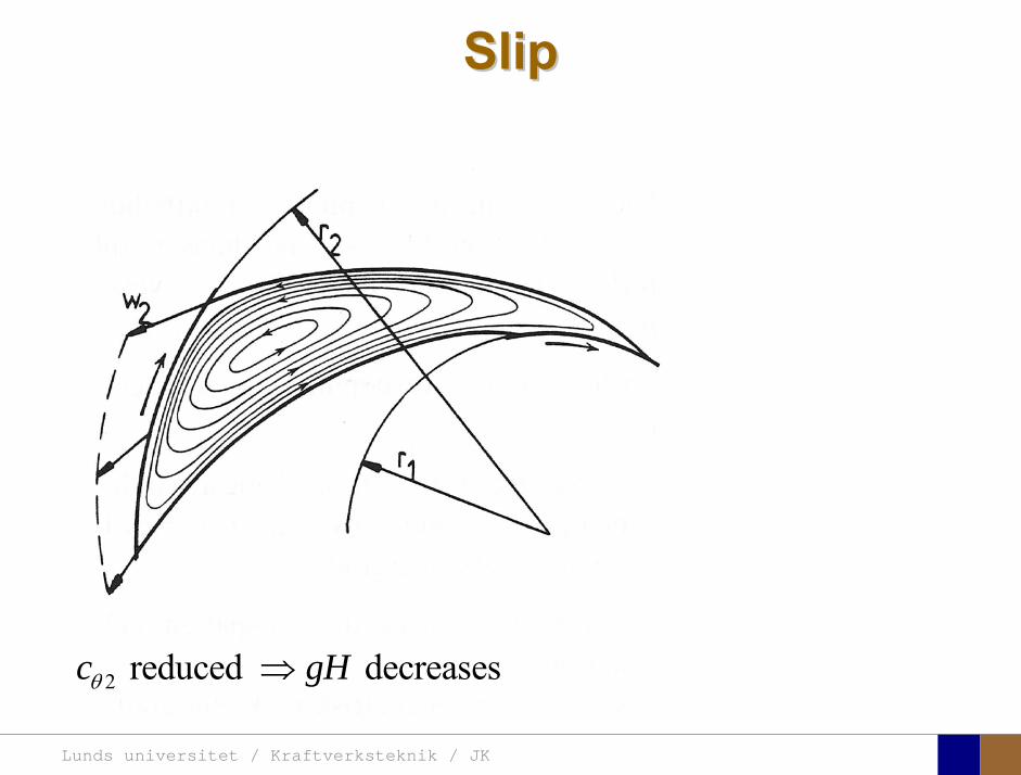
SlipSlip

2 reduced decreasesc gHθ ⇒

Lunds universitet / Kraftverksteknik / JK

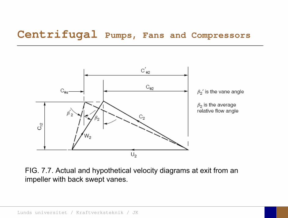
Centrifugal Pumps, Fans and Compressors

FIG. 7.7. Actual and hypothetical velocity diagrams at exit from an impeller with back swept vanes.

Lunds universitet / Kraftverksteknik / JK

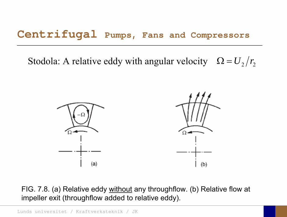
Centrifugal Pumps, Fans and Compressors

FIG. 7.8. (a) Relative eddy without any throughflow. (b) Relative flow at impeller exit (throughflow added to relative eddy).

Stodola: A relative eddy with angular velocity 2 2U rΩ =

Lunds universitet / Kraftverksteknik / JK

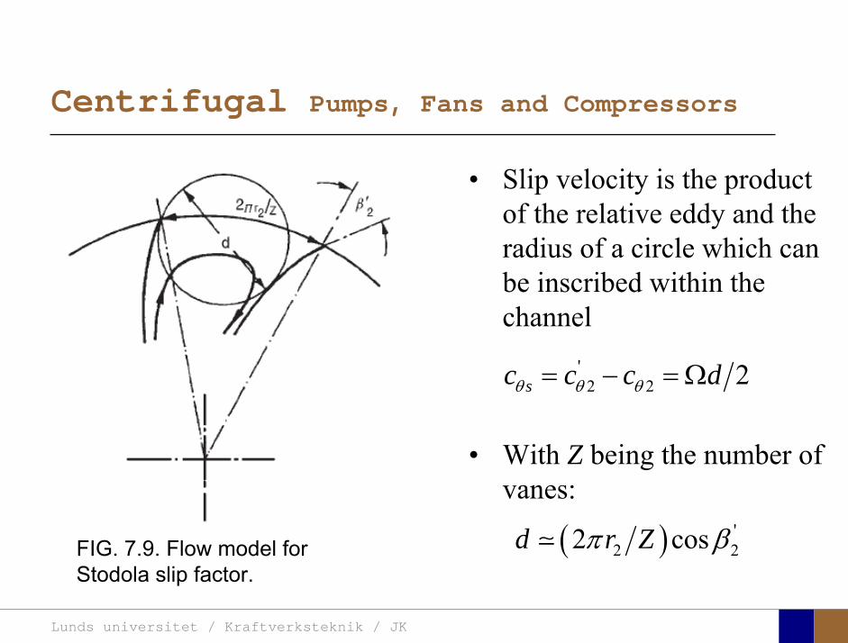
Centrifugal Pumps, Fans and Compressors

FIG. 7.9. Flow model for Stodola slip factor.

• Slip velocity is the product of the relative eddy and the radius of a circle which can be inscribed within the channel

• With Z being the number of vanes:

'2 2 2sc c c dθ θ θ= − = Ω

( ) '2 22 cosd r Zπ β

Lunds universitet / Kraftverksteknik / JK

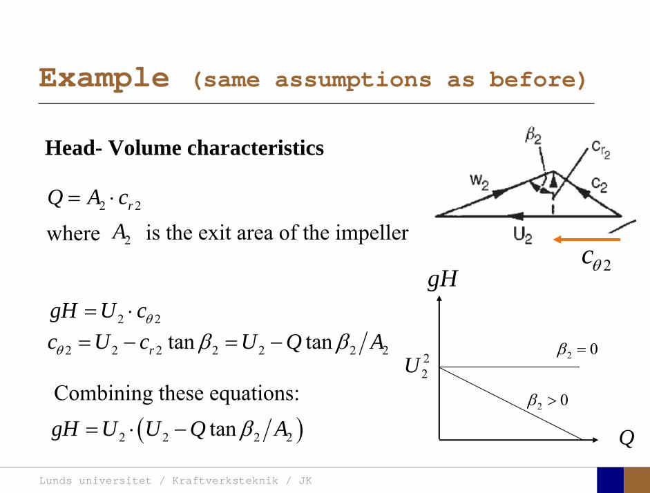
Example (same assumptions as before)

2 2rQ A c= ⋅

Head- Volume characteristics

where 2A is the exit area of the impeller 2cθ

2 2 2 2 2 2 2tan tanrc U c U Q Aθ β β= − = −2 2gH U cθ= ⋅

Combining these equations:

( )2 2 2 2tangH U U Q Aβ= ⋅ − Q

gH

22U

2 0β >

2 0β =

Lunds universitet / Kraftverksteknik / JK

Example

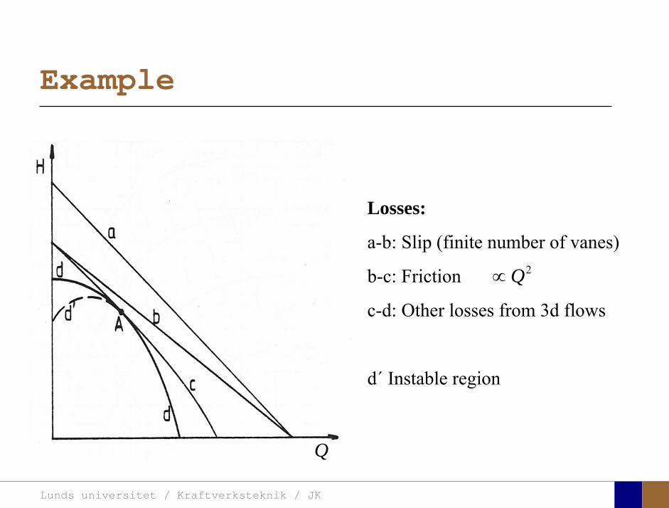
Losses:

a-b: Slip (finite number of vanes)

b-c: Friction

c-d: Other losses from 3d flows

d´ Instable region

2Q∝

Q

Lunds universitet / Kraftverksteknik / JK

Theory of turbo machinery / Turbomaskinernas teori

Dixon, chapter 9

Hydraulic Turbines 30° 49′ 15″ N, 111° 0′ 8″ E

Lunds universitet / Kraftverksteknik / JK

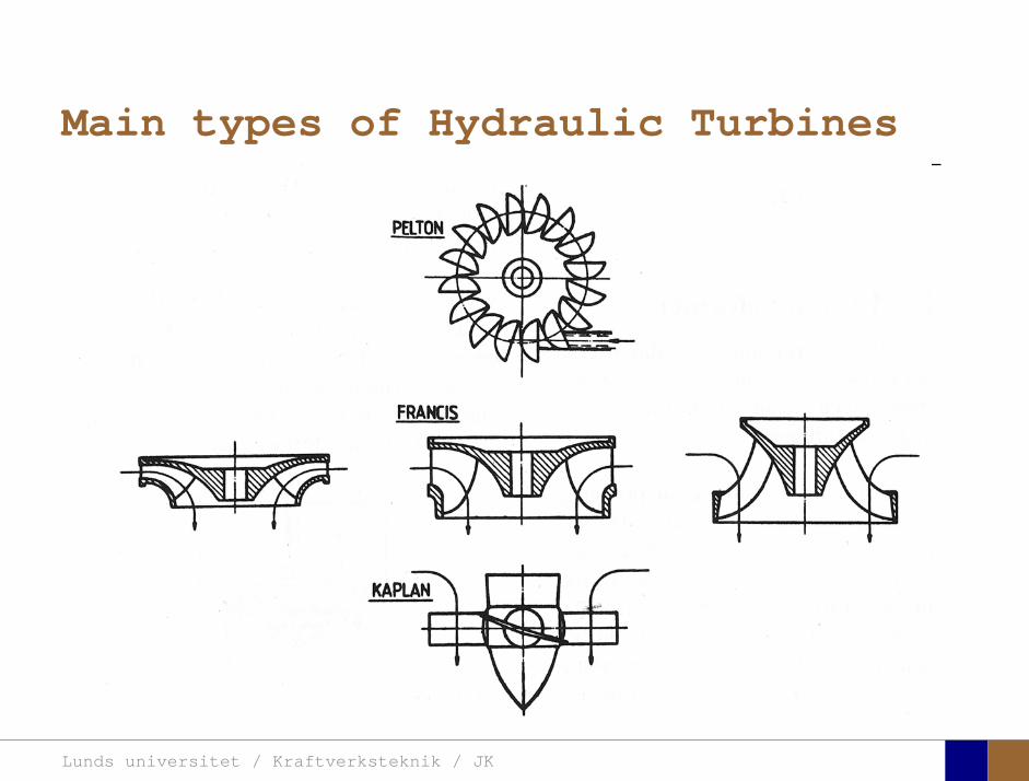
Main types of Hydraulic Turbines

Lunds universitet / Kraftverksteknik / JK

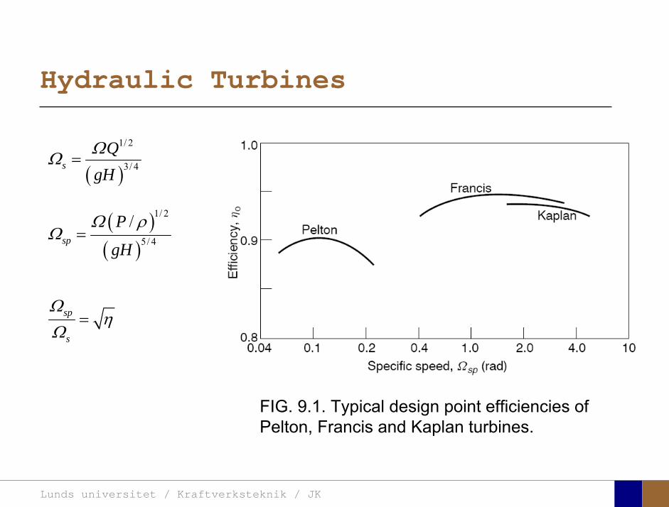
Hydraulic Turbines

sp

s

Ωη

Ω=

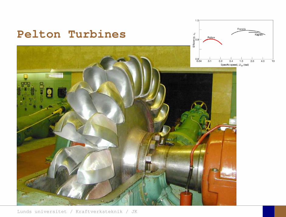
FIG. 9.1. Typical design point efficiencies of Pelton, Francis and Kaplan turbines.

sp

s

Ωη

Ω=

( )( )

1/ 2

5/ 4

/sp

P

gH

Ω ρΩ =

( )

1/ 2

3/ 4sQ

gHΩΩ =

Lunds universitet / Kraftverksteknik / JK

Hydraulic Turbines

Lunds universitet / Kraftverksteknik / JK

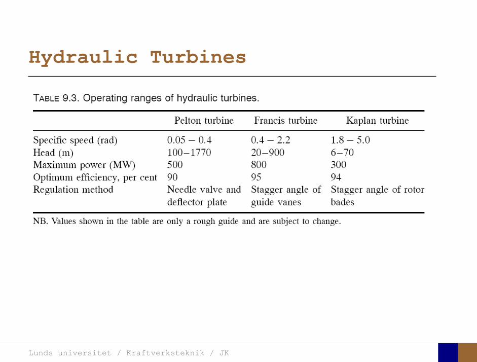
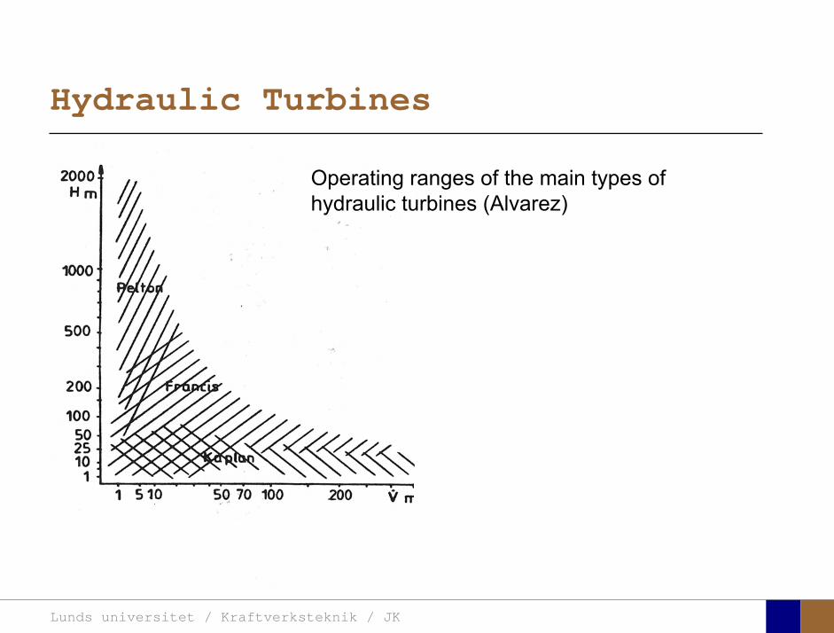
Hydraulic Turbines

Operating ranges of the main types of hydraulic turbines (Alvarez)

Lunds universitet / Kraftverksteknik / JK

Pelton Turbines

Lunds universitet / Kraftverksteknik / JK

Pelton Turbines

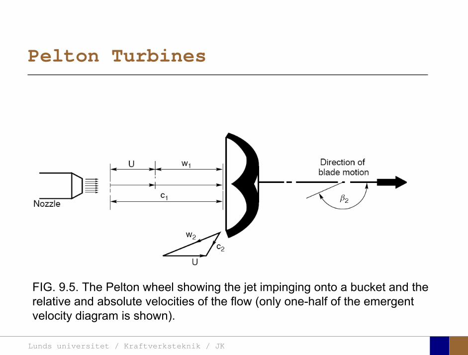
FIG. 9.5. The Pelton wheel showing the jet impinging onto a bucket and the relative and absolute velocities of the flow (only one-half of the emergentvelocity diagram is shown).

Lunds universitet / Kraftverksteknik / JK

Pelton Turbines

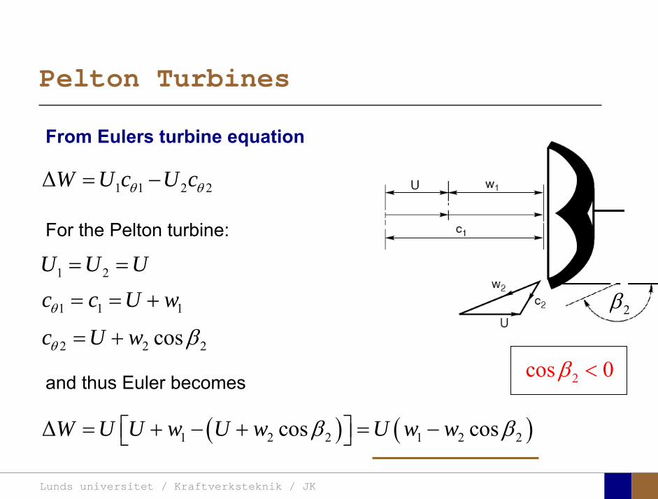
1 1 2 2ΔW U c U cθ θ= −

( ) ( )1 2 2 1 2 2Δ cos cosW U U w U w U w wβ β⎡ ⎤= + − + = −⎣ ⎦

From Eulers turbine equation

For the Pelton turbine:

1 2U U U= =

1 1 1c c U wθ

and thus Euler becomes

= = +

2 2 2cosc U wθ β= +2β

2cos 0β <

Lunds universitet / Kraftverksteknik / JK

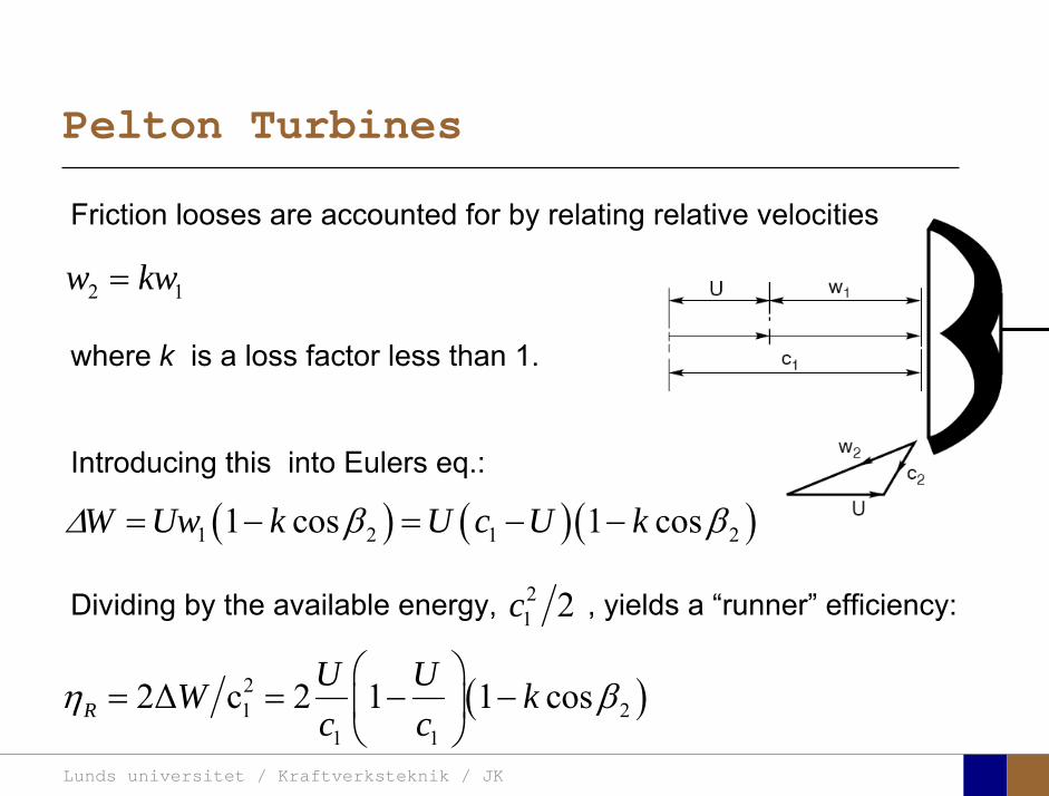
Pelton Turbines

2 1w kw=

where k is a loss factor less than 1.

Introducing this into Eulers eq.:

( )21 2

1 1

2Δ c 2 1 1 cosRU UW kc c

η β⎛ ⎞

= = − −⎜ ⎟⎝ ⎠

Dividing by the available energy, , yields a “runner” efficiency:

Friction looses are accounted for by relating relative velocities

21 2c

( ) ( )( )1 2 1 21 cos 1 cosW Uw k U c U kΔ β β= − = − −

Lunds universitet / Kraftverksteknik / JK

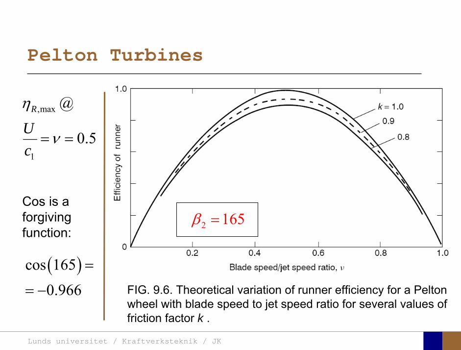
Pelton Turbines

FIG. 9.6. Theoretical variation of runner efficiency for a Pelton wheel with blade speed to jet speed ratio for several values of friction factor k .

2 165β =

,max

1

@

0.5

R

Uc

η

ν= =

Cos is a forgiving function:

( )cos 1650.966

=

= −

Lunds universitet / Kraftverksteknik / JK

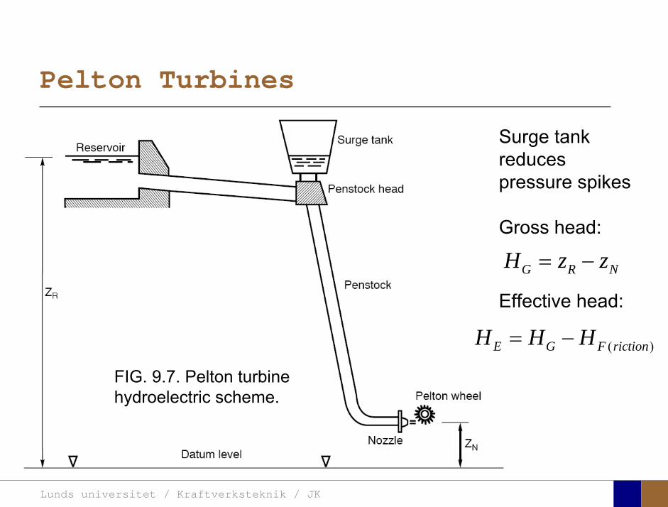
Pelton Turbines

FIG. 9.7. Pelton turbine hydroelectric scheme.

Surge tank reduces pressure spikes

Gross head:

G R NH z z= −

Effective head:

( )E G F rictionH H H= −

Lunds universitet / Kraftverksteknik / JK

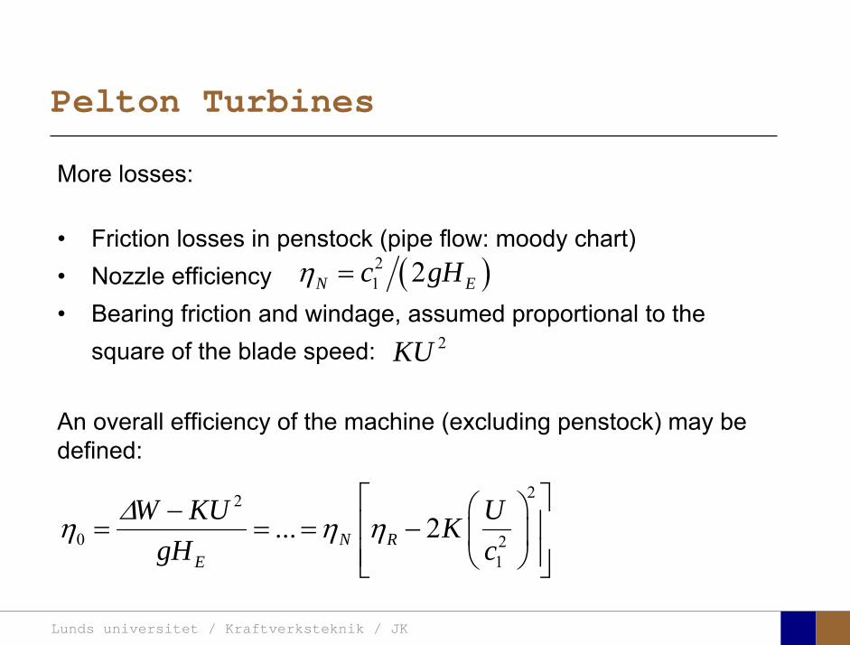
Pelton Turbines

More losses:

• Friction losses in penstock (pipe flow: moody chart)• Nozzle efficiency • Bearing friction and windage, assumed proportional to the

square of the blade speed:

( )21 2N Ec gHη =

2KU

An overall efficiency of the machine (excluding penstock) may bedefined:

22

0 21

... 2N RE

W KU UKgH c

Δη η η⎡ ⎤⎛ ⎞− ⎢ ⎥= = = − ⎜ ⎟⎢ ⎥⎝ ⎠⎣ ⎦

Lunds universitet / Kraftverksteknik / JK

Pelton Turbines

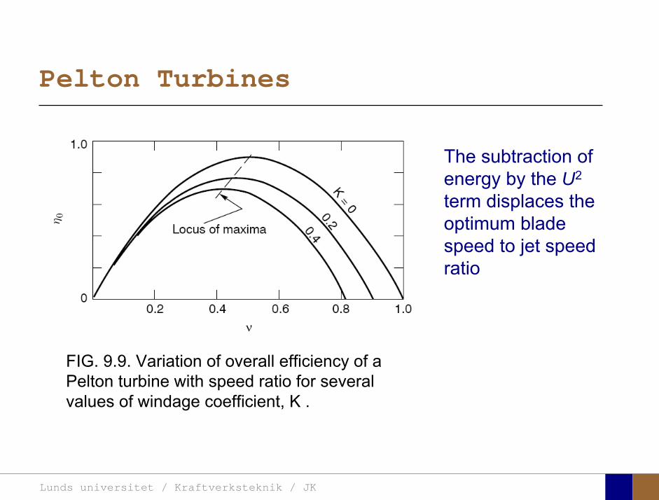
FIG. 9.9. Variation of overall efficiency of a Pelton turbine with speed ratio for severalvalues of windage coefficient, K .

The subtraction of energy by the U2

term displaces the optimum blade speed to jet speed ratio

Lunds universitet / Kraftverksteknik / JK

Pelton Turbines, controle

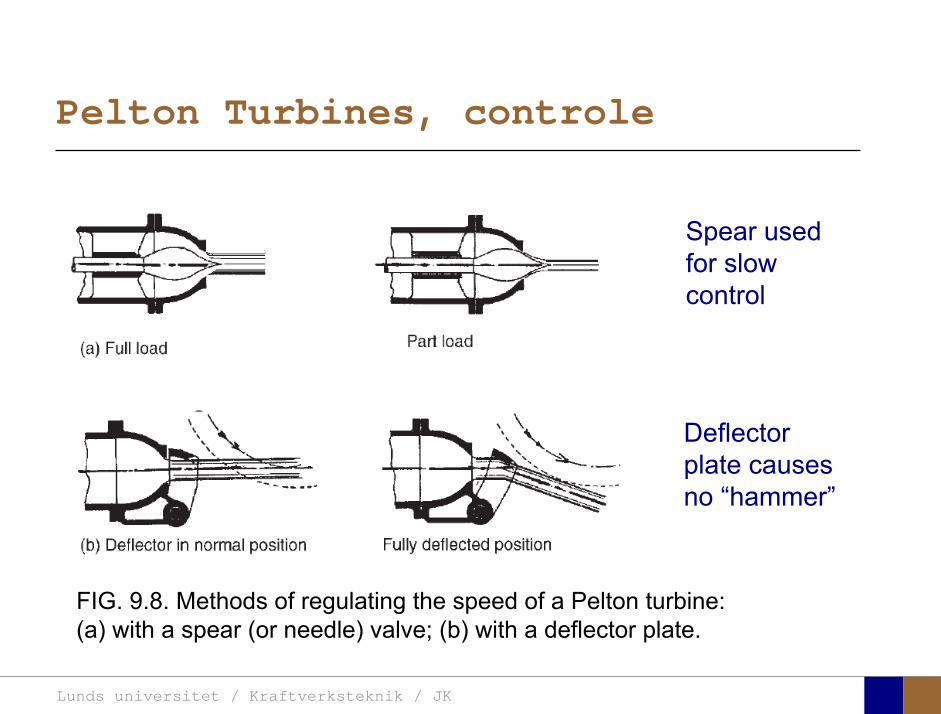
FIG. 9.8. Methods of regulating the speed of a Pelton turbine: (a) with a spear (or needle) valve; (b) with a deflector plate.

Spear used for slow control

Deflector plate causes no “hammer”

Lunds universitet / Kraftverksteknik / JK

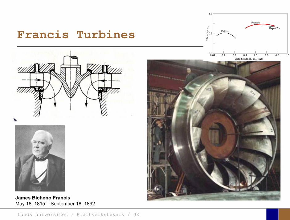
Francis Turbines

James Bicheno FrancisMay 18, 1815 – September 18, 1892

Lunds universitet / Kraftverksteknik / JK

Francis Turbines

Reaction turbines

Pressure drop takes place in the turbine itselfWater flow completely fills all part of the turbinePivotable guide vanes are used for control (Francis)A draft tube is normally added on to the exit; it is considered an integral part of the turbine

Lunds universitet / Kraftverksteknik / JK

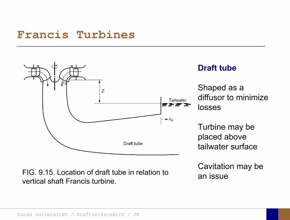
Francis Turbines

FIG. 9.15. Location of draft tube in relation to vertical shaft Francis turbine.

Draft tube

Shaped as a diffusor to minimize losses

Turbine may be placed above tailwater surface

Cavitation may be an issue

Lunds universitet / Kraftverksteknik / JK

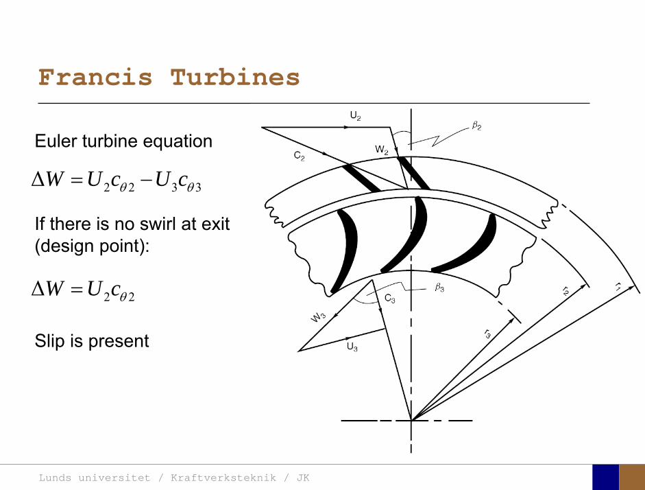
Francis Turbines

Euler turbine equation

2 2 3 3ΔW U c U cθ θ= −

2 2ΔW U c

If there is no swirl at exit (design point):

θ=

Slip is present

Lunds universitet / Kraftverksteknik / JK

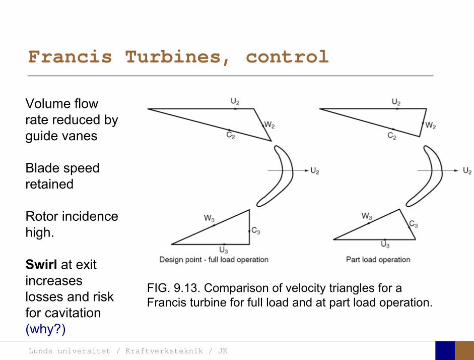
Francis Turbines, control

FIG. 9.13. Comparison of velocity triangles for a Francis turbine for full load and at part load operation.

Volume flow rate reduced by guide vanes

Blade speed retained

Rotor incidence high.

Swirl at exit increases losses and risk for cavitation(why?)

Lunds universitet / Kraftverksteknik / JK

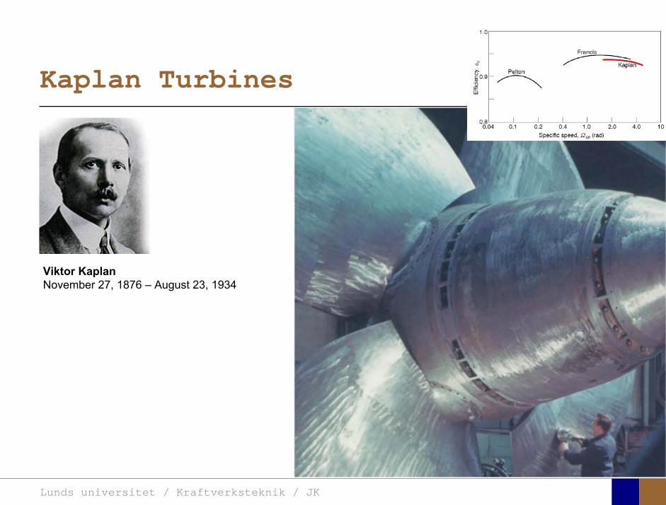
Kaplan Turbines

Viktor KaplanNovember 27, 1876 – August 23, 1934

Lunds universitet / Kraftverksteknik / JK

Francis Turbines

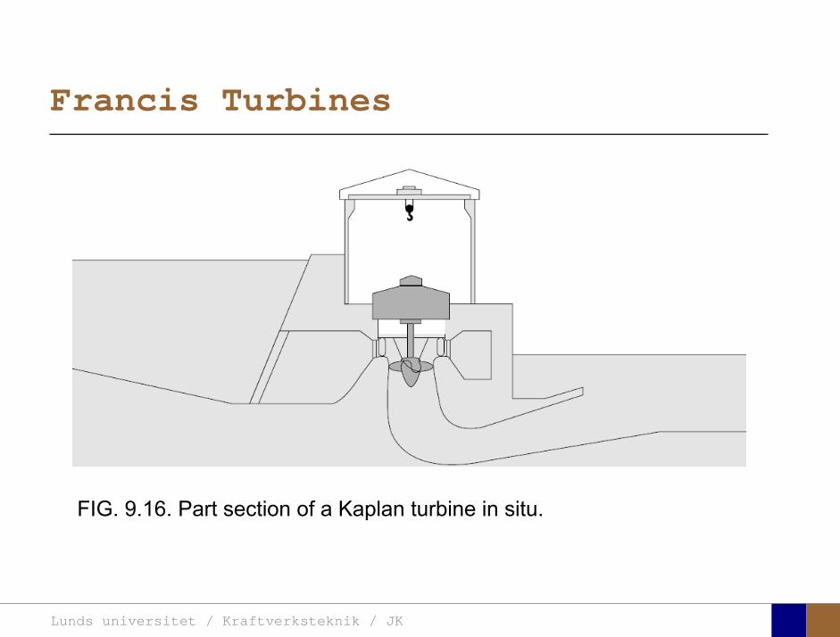
FIG. 9.16. Part section of a Kaplan turbine in situ.

Lunds universitet / Kraftverksteknik / JK

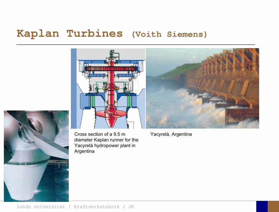
Kaplan Turbines (Voith Siemens)

Cross section of a 9.5 m diameter Kaplan runner for the Yacyretá hydropower plant in Argentina

Yacyretà, Argentina

Lunds universitet / Kraftverksteknik / JK

Kaplan Turbines

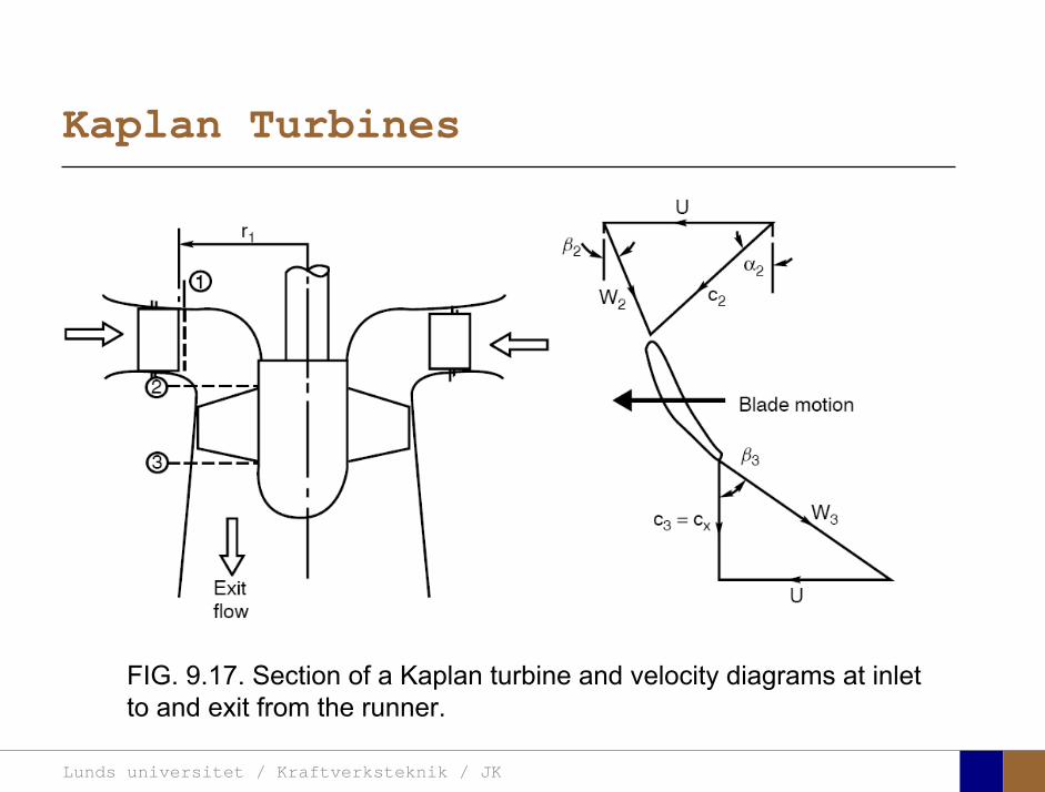
FIG. 9.17. Section of a Kaplan turbine and velocity diagrams at inlet to and exit from the runner.

Lunds universitet / Kraftverksteknik / JK

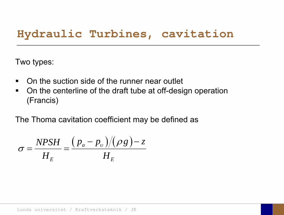
Hydraulic Turbines, cavitation

Two types:

On the suction side of the runner near outletOn the centerline of the draft tube at off-design operation (Francis)

The Thoma cavitation coefficient may be defined as

( ) ( )a

E E

p p g zNPSHH H

υ ρσ

− −= =

Lunds universitet / Kraftverksteknik / JK

Theory of turbo machinery / Turbomaskinernas teori

Dixon, chapter 10

Wind Turbines

Lunds universitet / Kraftverksteknik / JK

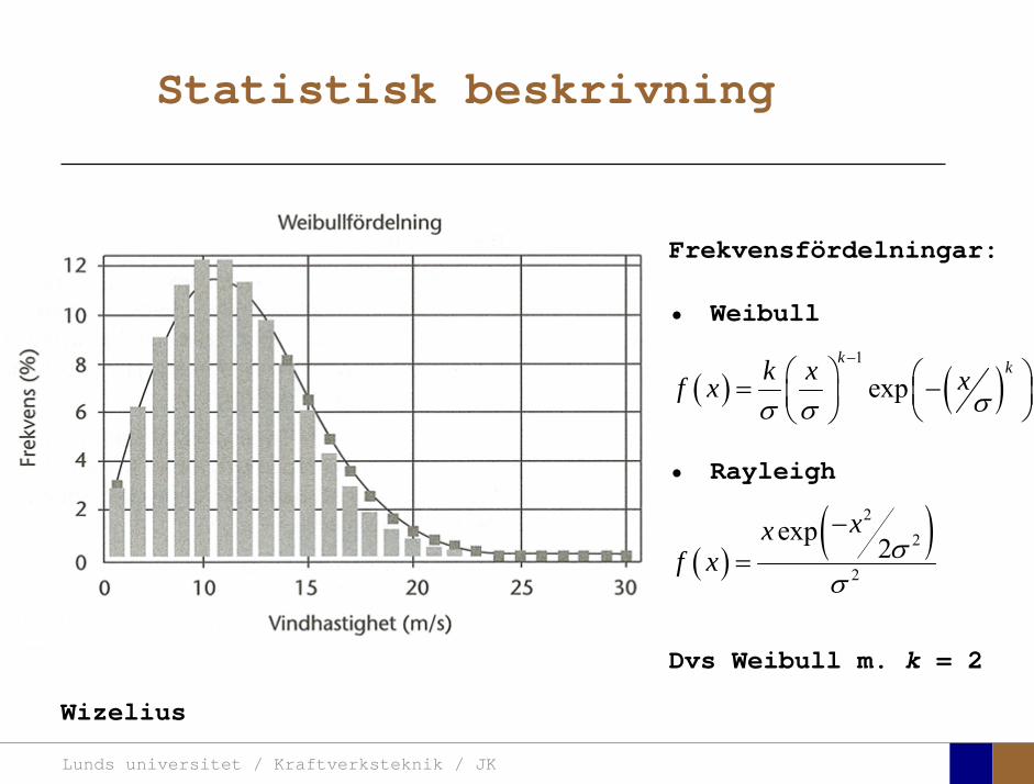
Statistisk beskrivning

Wizelius

Frekvensfördelningar:

• Weibull

• Rayleigh

Dvs Weibull m. k = 2

( )( )2

2

2

exp 2xx

f x σσ

−=

( ) ( )1

expk kk x xf x σσ σ

−⎛ ⎞ ⎛ ⎞= −⎜ ⎟⎜ ⎟ ⎝ ⎠⎝ ⎠

Lunds universitet / Kraftverksteknik / JK

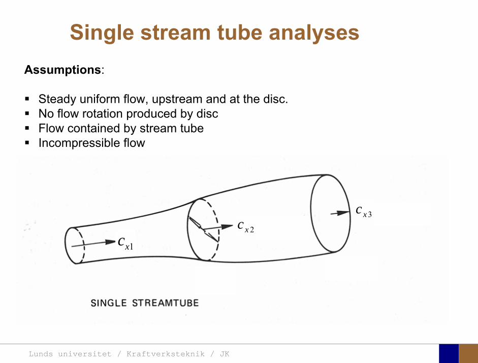
Single stream tube analyses

1xc2xc

3xc

Assumptions:

Steady uniform flow, upstream and at the disc.No flow rotation produced by discFlow contained by stream tubeIncompressible flow

Lunds universitet / Kraftverksteknik / JK

Mass flow 2 2xm c Aρ=

Single stream tube analyses

Axial force ( )1 3x xX m c c= −

Energy loss of the wind ( )2 21 3 2W x xP m c c= −

Disk power ( )2 1 3 2x x x xP Xc m c c c= = −

Setting :WP P=

( ) ( ) ( )2 21 3 2 1 3 2 1 32 2x x x x x x x xm c c c m c c c c c− = − ⇒ = +

Lunds universitet / Kraftverksteknik / JK

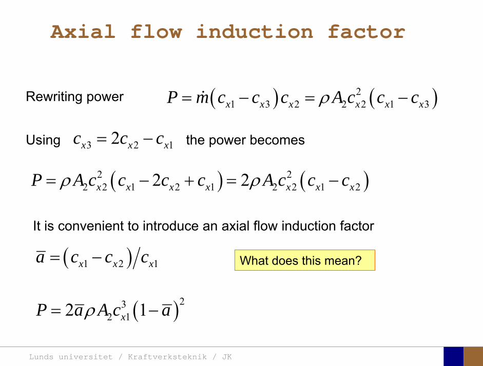
Axial flow induction factor

Rewriting power ( ) ( )21 3 2 2 2 1 3x x x x x xP m c c c A c c cρ= − = −

Using 3 2 12x x xc c c= − the power becomes

( ) ( )2 22 2 1 2 1 2 2 1 22 2x x x x x x xP A c c c c A c c cρ ρ= − + = −

It is convenient to introduce an axial flow induction factor

( )1 2 1x x xa c c c= −

( )232 12 1xP a A c aρ= −

What does this mean?

Lunds universitet / Kraftverksteknik / JK

The power coefficient

max 1 2xQ c A=

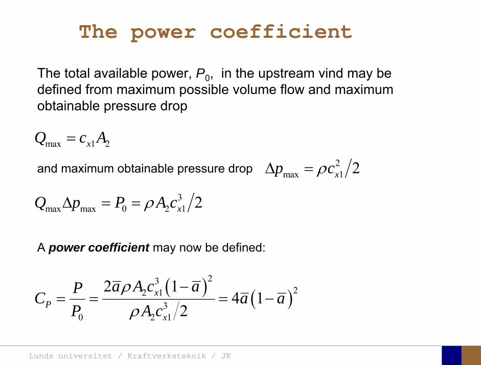
The total available power, P0, in the upstream vind may be defined from maximum possible volume flow and maximum obtainable pressure drop

and maximum obtainable pressure drop 2max 1 2xp cρΔ =

3max max 0 2 1 2xQ p P A cρΔ = =

A power coefficient may now be defined:

( ) ( )23

22 13

0 2 1

2 14 1

2x

Px

a A c aPC a aP A c

ρρ

−= = = −

Lunds universitet / Kraftverksteknik / JK

Wind Turbines

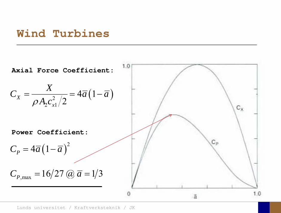
( )22 1

4 12X

x

XC a aA cρ

= = −

Axial Force Coefficient:

( )24 1PC a a= −

Power Coefficient:

,max 16 27 @ 1 3PC a= =

Lunds universitet / Kraftverksteknik / JK

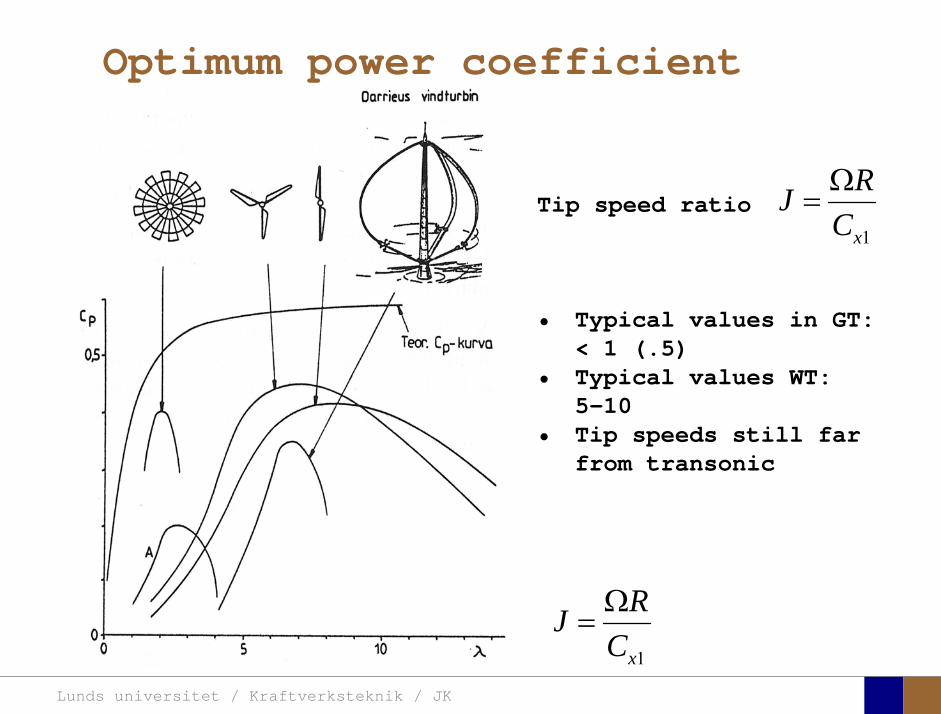
Optimum power coefficient

1x

RJCΩ

=

Tip speed ratio

• Typical values in GT:< 1 (.5)

• Typical values WT:5-10

• Tip speeds still far from transonic

1x

RJCΩ

=

Lunds universitet / Kraftverksteknik / JK

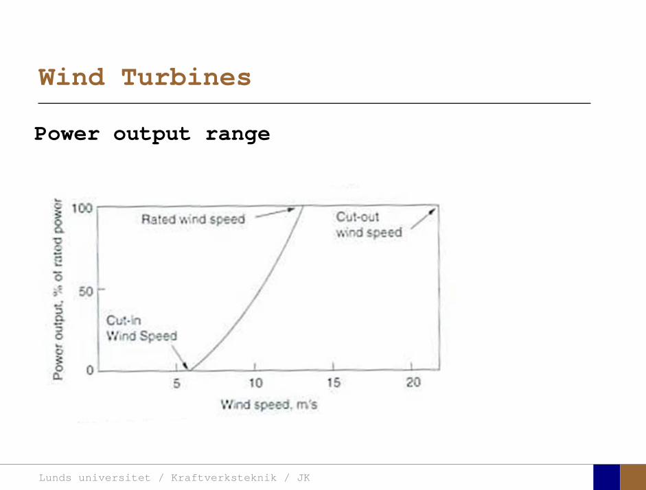
Wind Turbines

Power output range

Lunds universitet / Kraftverksteknik / JK

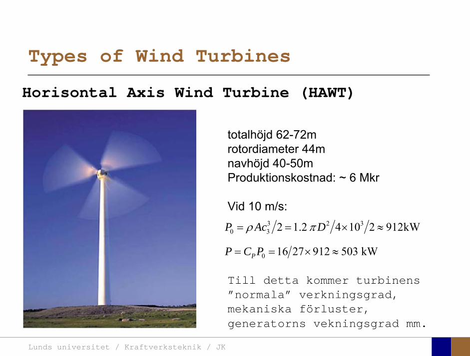
Types of Wind Turbines

Horisontal Axis Wind Turbine (HAWT)

totalhöjd 62-72mrotordiameter 44mnavhöjd 40-50mProduktionskostnad: ~ 6 Mkr

Vid 10 m/s:3 2 3

0 3 2 1.2 4 10 2 912kWP Ac Dρ π= = × ≈

0 16 27 912 503 kWPP C P= = × ≈

Till detta kommer turbinens ”normala” verkningsgrad, mekaniska förluster, generatorns vekningsgrad mm.

Lunds universitet / Kraftverksteknik / JK

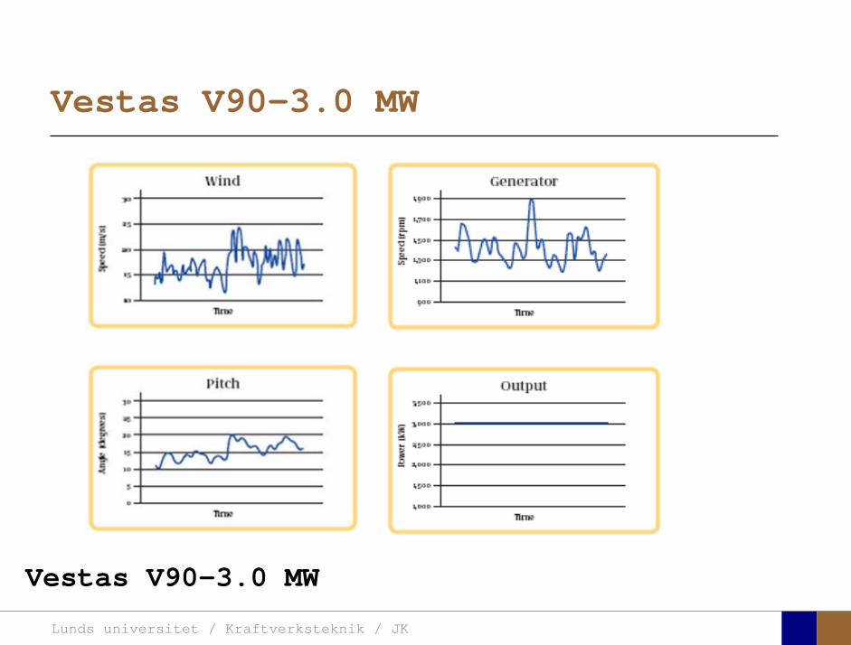
Vestas V90-3.0 MW

Vestas V90-3.0 MW

Lunds universitet / Kraftverksteknik / JK

Theory of turbo machinery / Turbomaskinernas teori

Gas turbines

Lunds universitet / Kraftverksteknik / JK

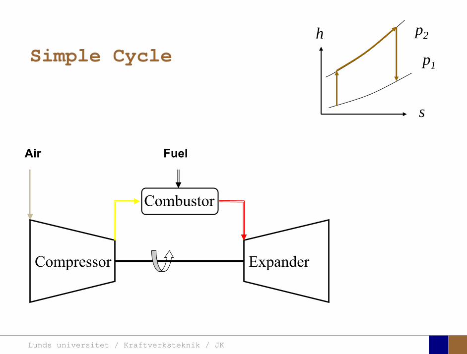
Simple Cycle

Compressor

h

Expander

s

p1

p2

Air

Combustor

Fuel

Lunds universitet / Kraftverksteknik / JK

Ideal Cycle

a) Compression and expansion are reversible and adiabatic, i.e. isentropic

b) The change of kinetic energy of the working fluid between the inlet and outlet of each component is negligable.

c) Pressure losses are neglected.d) The working fluid is the same in the entire cycle and it is a

perfect gas with constant specific heats.e) The mass flow of gas is the same throughout the cyclef) The heat-exhanger is a counterflow type with “complete”

heat transfer

Lunds universitet / Kraftverksteknik / JK

Ideal Cycle

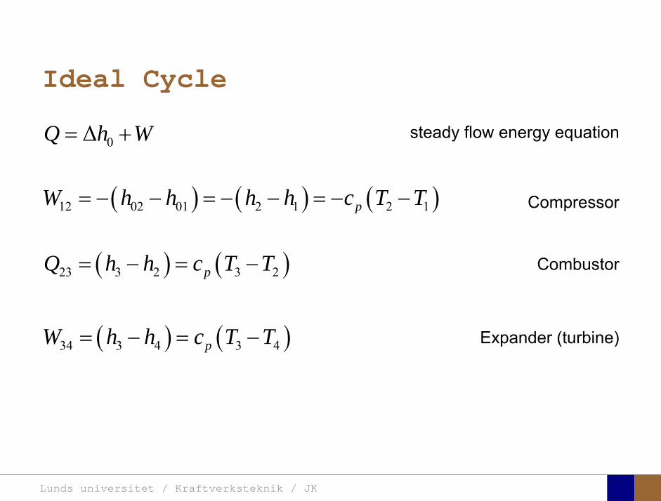
0ΔQ h W= +

( ) ( ) ( )12 02 01 2 1 2 1pW h h h h c T T= − − = − − = − −

( ) ( )23 3 2 3 2pQ h h c T T= − = −

( ) ( )34 3 4 3 4pW h h c T T= − = −

Compressor

Combustor

Expander (turbine)

steady flow energy equation

Lunds universitet / Kraftverksteknik / JK

Ideal Cycle

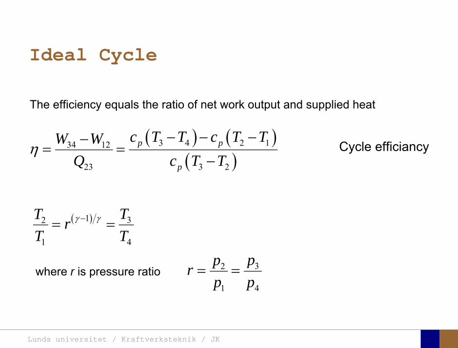
( )1 32

1 4

TT rT T

γ γ−= =

32

1 4

pprp p

= =where r is pressure ratio

The efficiency equals the ratio of net work output and supplied heat

( ) ( )( )

3 4 2 134 12

23 3 2

p p

p

c T T c T TW WQ c T T

η− − −−

= =−

Cycle efficiancy

Lunds universitet / Kraftverksteknik / JK

Ideal Cycle

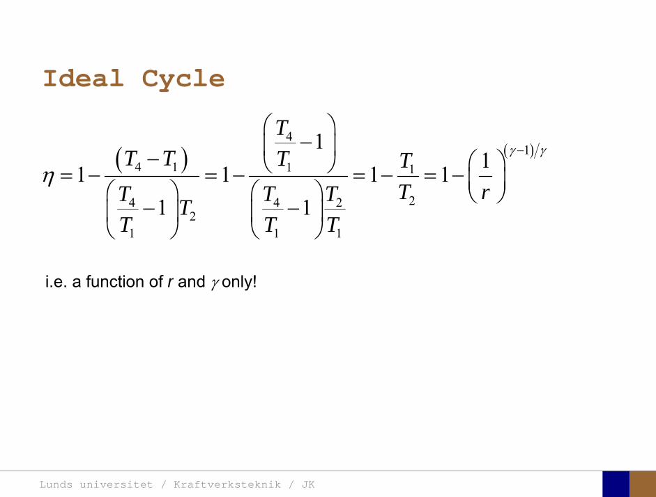
( ) ( )4

14 1 1 1

24 4 22

1 1 1

111 1 1 1

1 1

TT T T T

T rT T TTT T T

γ γ

η−

⎛ ⎞−⎜ ⎟− ⎛ ⎞⎝ ⎠= − = − = − = − ⎜ ⎟⎛ ⎞ ⎛ ⎞ ⎝ ⎠− −⎜ ⎟ ⎜ ⎟

⎝ ⎠ ⎝ ⎠

i.e. a function of r and γ only!

Lunds universitet / Kraftverksteknik / JK

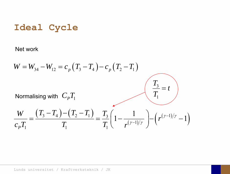
Ideal Cycle

( ) ( )( )

( )( )13 4 2 1 31

1 1 1

11 1P

T T T T TW rc T T T r

γ γγ γ

−−

− − − ⎛ ⎞= = − − −⎜ ⎟⎝ ⎠

( ) ( )34 12 3 4 2 1p pW W W c T T c T T= − = − − −

Normalising with 1PC T

Net work

3

1

T tT

=

Lunds universitet / Kraftverksteknik / JK2009-10-19 Magnus Genrup 110

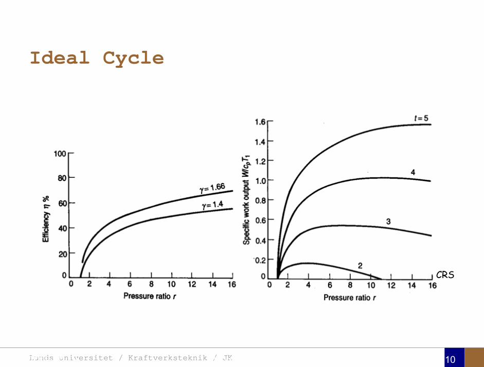
CRS

Ideal Cycle

Lunds universitet / Kraftverksteknik / JK

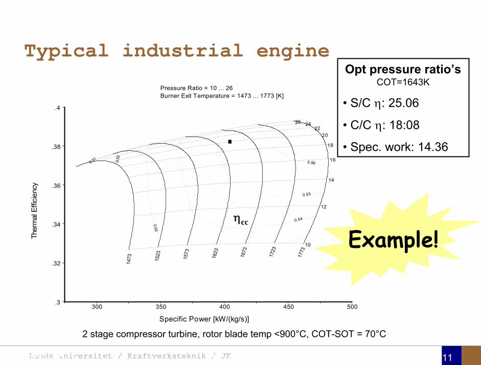
Typical industrial engine

2009-10-19 Magnus Genrup 111

Opt pressure ratio’sCOT=1643K

• S/C η: 25.06

• C/C η: 18:08

• Spec. work: 14.36

2 stage compressor turbine, rotor blade temp <900°C, COT-SOT = 70°C

.3

.32

.34

.36

.38

.4

Ther

mal

Effi

cien

cy

300 350 400 450 500

Specific Power [kW/(kg/s)]

Pressure Ratio = 10 ... 26 Burner Exit Temperature = 1473 ... 1773 [K]

147

3

152

3

157

3

162

3

167

3

172

3

177

3

0.51 0.52

0.53

0.54

0.55

0.56

Dotted Lines = (PWSD*0.985*0.985+cp_val7)/(WF* [g/(kN*s)]

10

12

14

16

18

20 22

24 26 WCLTq2 iterated for T_m_T=1173ZW2Rstd iterated for W2=100WCLNq2 iterated for cp_val1=70

Example!ηcc

Lunds universitet / Kraftverksteknik / JK

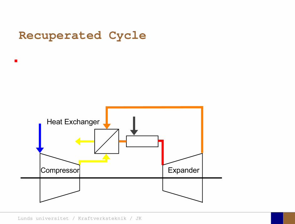
Recuperated Cycle

Compressor Expander

Heat Exchanger

Lunds universitet / Kraftverksteknik / JK

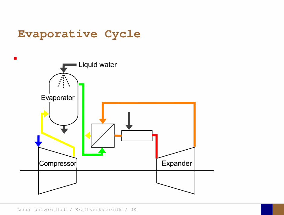
Evaporative Cycle

Compressor Expander

Liquid water

Evaporator

Lunds universitet / Kraftverksteknik / JK

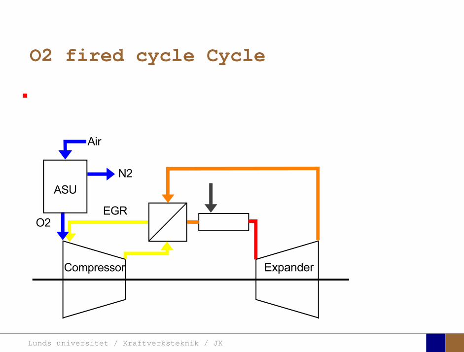
O2 fired cycle Cycle

ASU

Air

O2

N2

Compressor Expander

EGR

Lunds universitet / Kraftverksteknik / JK

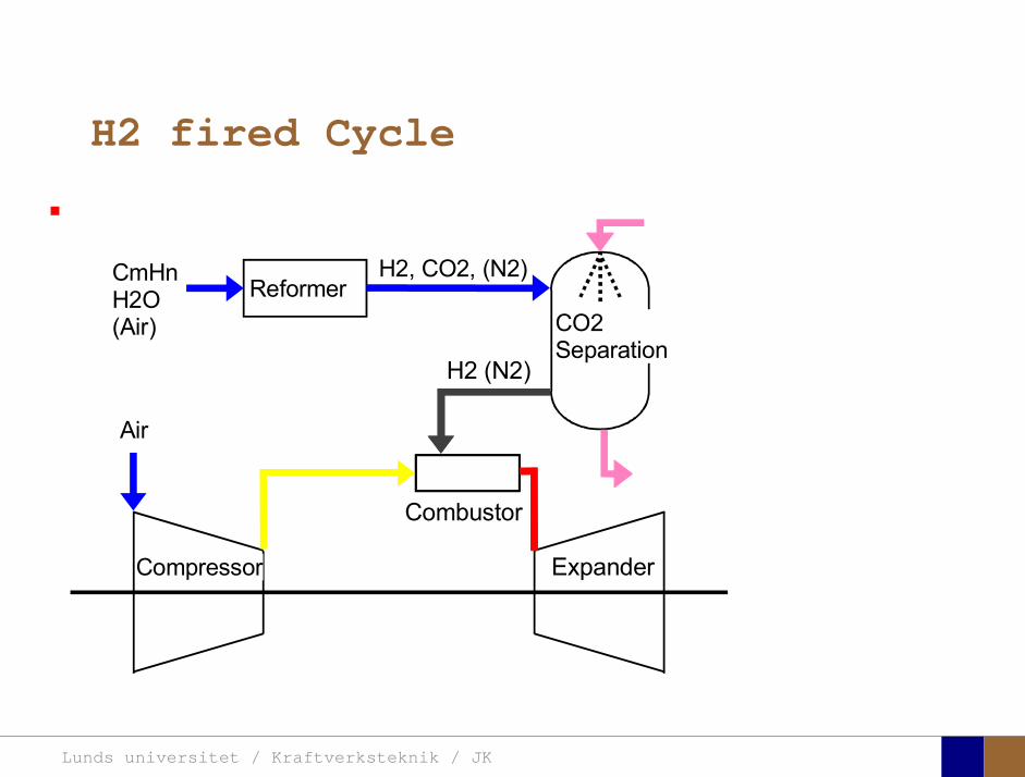
H2 fired Cycle

Reformer

Air

CmHnH2O(Air)

Compressor Expander

H2, CO2, (N2)

CO2Separation

Combustor

H2 (N2)

Lunds universitet / Kraftverksteknik / JK

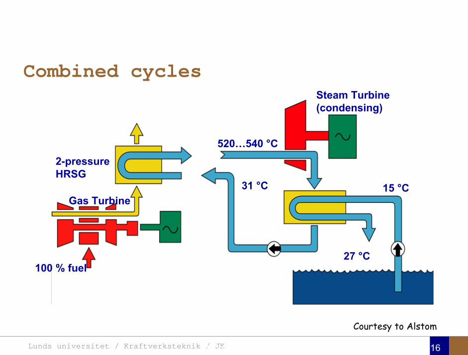
Combined cycles

Magnus Genrup 116

Steam Turbine (condensing)

100 % fuel

15 °CGas Turbine

2-pressure HRSG

520…540 °C

27 °C

31 °C

Courtesy to Alstom

Lunds universitet / Kraftverksteknik / JK

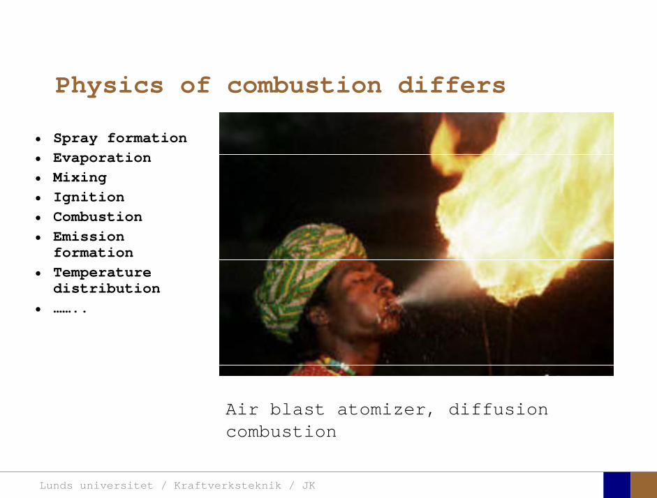
Physics of combustion differs

• Spray formation• Evaporation• Mixing• Ignition• Combustion• Emission

formation• Temperature

distribution• ……..

Air blast atomizer, diffusion combustion