
γλώσσες
Σελίδες
Νομικός


MATH 4245 - FALL 2012
Theory of Ordinary Differential Equations
Stability and Bifurcation II
John A. Burns
Center for Optimal Design And Control
Interdisciplinary Center for Applied Mathematics
Virginia Polytechnic Institute and State University Blacksburg, Virginia 24061-0531
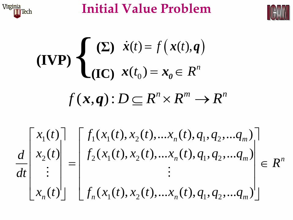
0( ) nt R 0x x(IC)
( ) ( ),t f tx x q(Σ) {(IVP)
( , ) : n m nf D R R Rx q
1 1 1 2 1 2
2 2 1 2 1 2
1 2 1 2
( ) ( ( ), ( ),... ( ), , ,... )
( ) ( ( ), ( ),... ( ), , ,... )
( ) ( ( ), ( ),... ( ), , ,... )
n m
n m n
n n n m
x t f x t x t x t q q q
x t f x t x t x t q q qdR
dt
x t f x t x t x t q q q
Initial Value Problem
0( ) nt R 0x x(IC)
( ) ( ),t f tx x q(Σ) {(IVP)
( , ) : n m nf D R R R x q
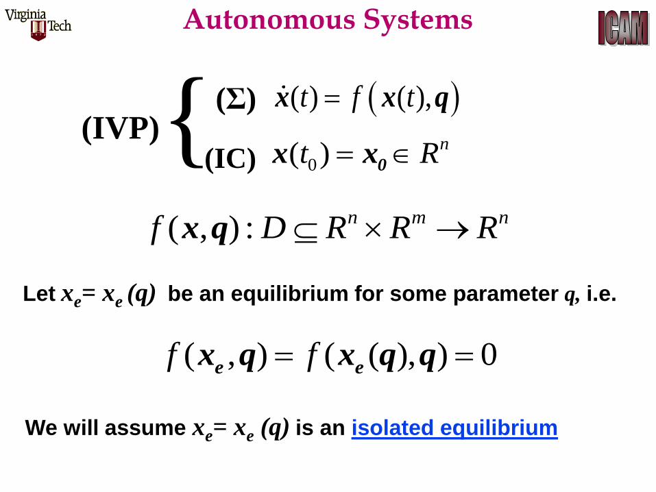
( , ) ( ( ), ) 0 f fe ex q x q q
Let xe= xe (q) be an equilibrium for some parameter q, i.e.
We will assume xe= xe (q) is an isolated equilibrium
Autonomous Systems
nR( )2
x q
Isolated Equilibrium
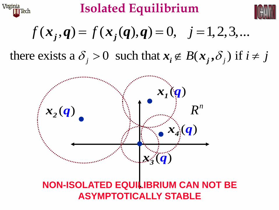
( , ) ( ( ), ) 0, 1,2,3,... f f jj jx q x q q
( )1
x q
( )3
x q
( )4
x q
there exists a 0 such that ( ) if j jB i ji jx x ,
NON-ISOLATED EQUILIBRIUM CAN NOT BE
ASYMPTOTICALLY STABLE
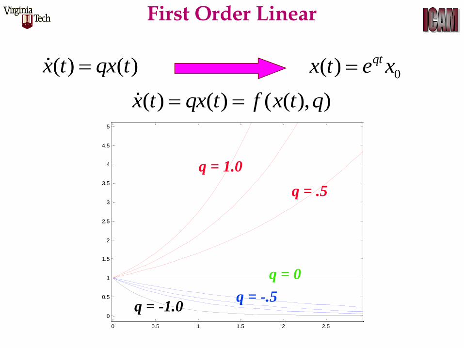
( ) ( )x t qx t0( ) qtx t e x
0 0.5 1 1.5 2 2.5
0
0.5
1
1.5
2
2.5
3
3.5
4
4.5
5
( ) ( ) ( ( ), ) x t qx t f x t q
q = 0
q = 1.0
q = -.5
q = .5
q = -1.0
First Order Linear
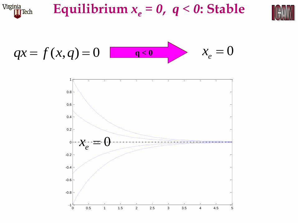
( , ) 0 qx f x q 0ex
0 0.5 1 1.5 2 2.5 3 3.5 4 4.5 5-1
-0.8
-0.6
-0.4
-0.2
0
0.2
0.4
0.6
0.8
1
0ex
q < 0
Equilibrium xe = 0, q < 0: Stable
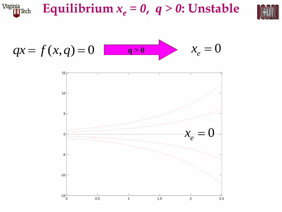
( , ) 0 qx f x q 0ex q > 0
0 0.5 1 1.5 2 2.5-15
-10
-5
0
5
10
15
0ex
Equilibrium xe = 0, q > 0: Unstable
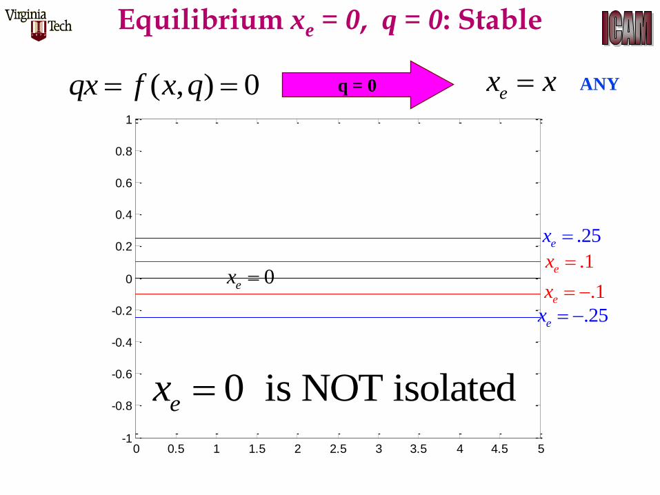
Equilibrium xe = 0, q = 0: Stable
0 0.5 1 1.5 2 2.5 3 3.5 4 4.5 5-1
-0.8
-0.6
-0.4
-0.2
0
0.2
0.4
0.6
0.8
1
0ex
( , ) 0 qx f x q ex xq = 0
.25ex
.25ex
.1ex
.1ex
ANY
0 is NOT isolatedex
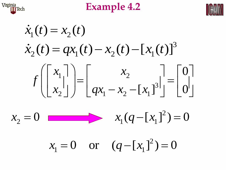
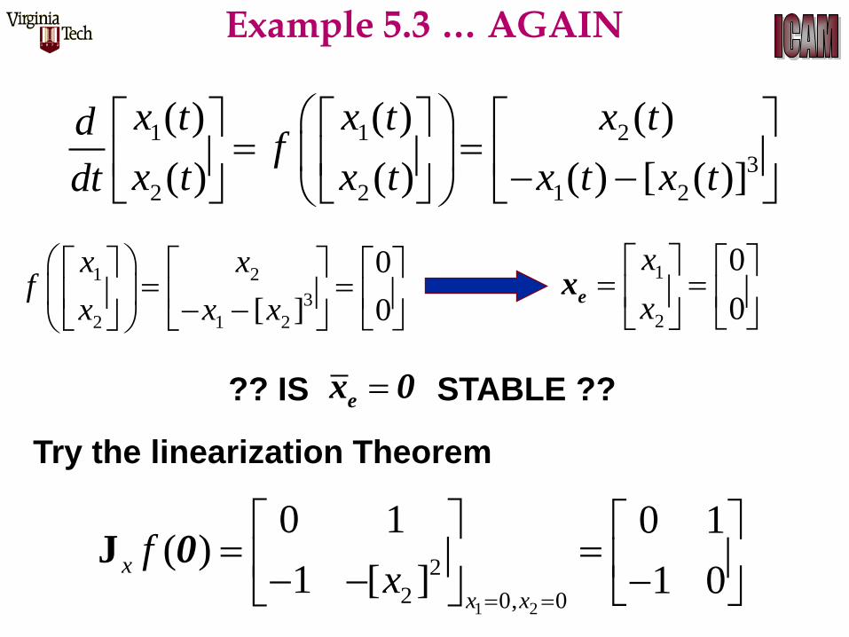
1 2( ) ( )x t x t3
2 1 2 1( ) ( ) ( ) [ ( )] x t qx t x t x t
1 2
3
2 1 2 1
0
[ ] 0
x xf
x qx x x
2 0x 2
1 1( [ ] ) 0 x q x
2
1 10 or ( [ ] ) 0 x q x
Example 4.2
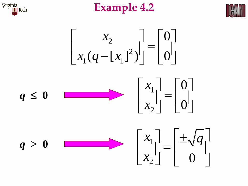
2
2
1 1
0
( [ ] ) 0
x
x q x
1
2
0
0
x
x
q 0
1
2 0
x q
xq > 0
Example 4.2
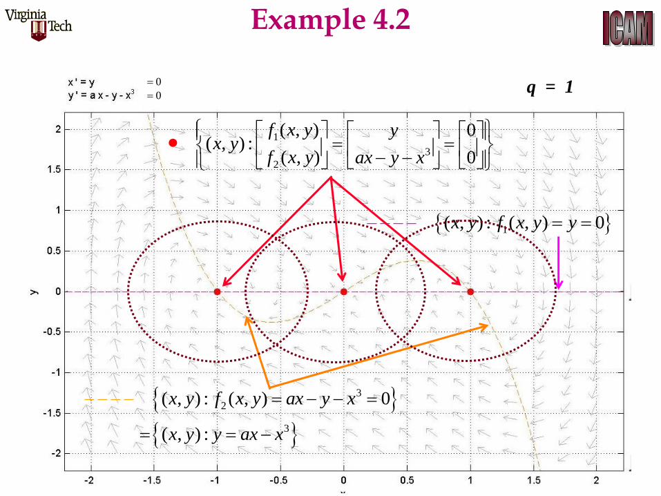
1 ( , ) : ( , ) 0x y f x y y
3
2
3
( , ) : ( , ) 0
( , ) :
x y f x y ax y x
x y y ax x
1
3
2
( , ) 0 ( , ) :
( , ) 0
f x y yx y
f x y ax y x
0
0
Example 4.2
q = 1

Epidemic Models
Susceptible Infected
Removed
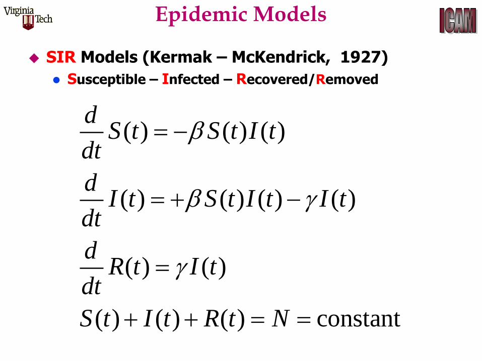
Epidemic Models
SIR Models (Kermak – McKendrick, 1927)
Susceptible – Infected – Recovered/Removed
( ) ( ) ( )
( ) ( ) ( ) ( )
( ) ( )
( ) ( ) ( ) constant
dS t S t I t
dt
dI t S t I t I t
dt
dR t I t
dt
S t I t R t N

SIR Models
( ) ( ) ( )
( ) ( ) ( ) ( ) ( ) ( )
dS t S t I t
dt
dI t S t I t I t I t S t
dt
( ) ( ) and ( ) ( ) ( ) constant d
R t I t S t I t R t Ndt
1 1 1 2
2 1 1 2 2 2
( ) ( ) ( )
( ) ( ) ( ) ( )
x t q x t x td
x t q x t x t q x tdt
1 2( ) ( ), ( ) ( ) and T
x t S t x t I t q
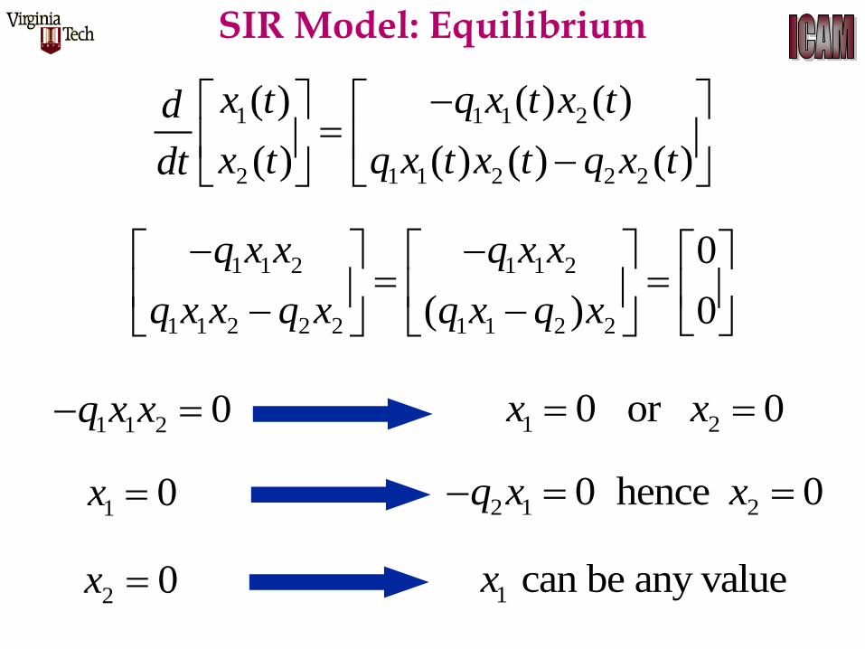
SIR Model: Equilibrium
1 1 1 2
2 1 1 2 2 2
( ) ( ) ( )
( ) ( ) ( ) ( )
x t q x t x td
x t q x t x t q x tdt
1 1 2 1 1 2
1 1 2 2 2 1 1 2 2
0
( ) 0
q x x q x x
q x x q x q x q x
1 1 2 0 q x x 1 20 or 0 x x
2 1 20 hence 0 q x x1 0x
1 can be any valuex2 0x
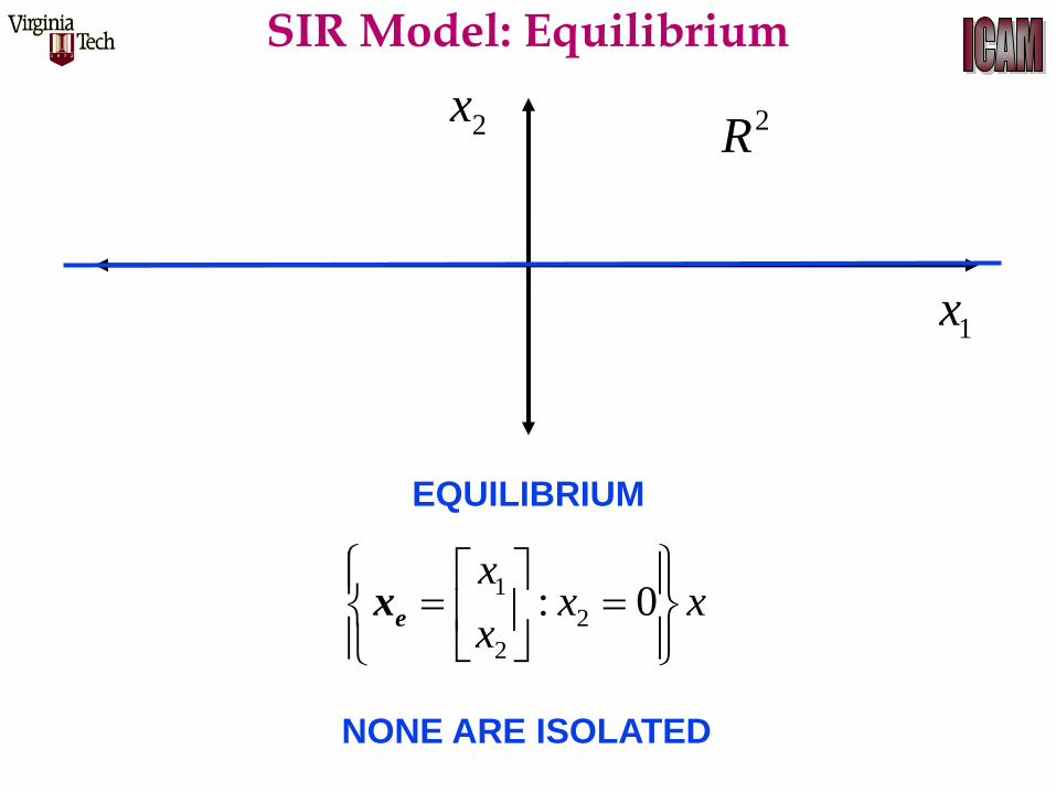
SIR Model: Equilibrium
NONE ARE ISOLATED
2R
1x
2x
EQUILIBRIUM
1
2
2
: 0
xx x
xex
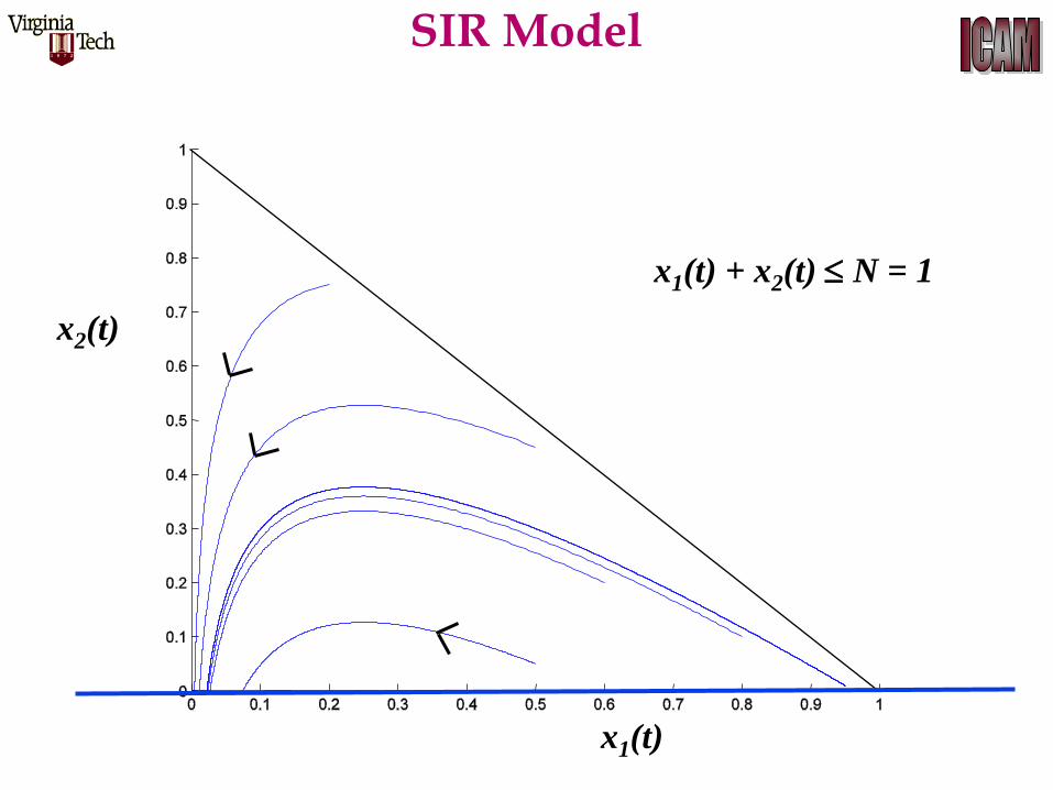
SIR Model
x2(t)
x1(t)
x1(t) + x2(t) N = 1
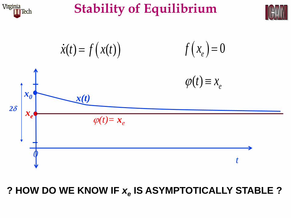
( ) ( )x t f x t 0ef x
x0
2
t
0
xe
(t)= xe
x(t)
( ) et x
? HOW DO WE KNOW IF xe IS ASYMPTOTICALLY STABLE ?
Stability of Equilibrium
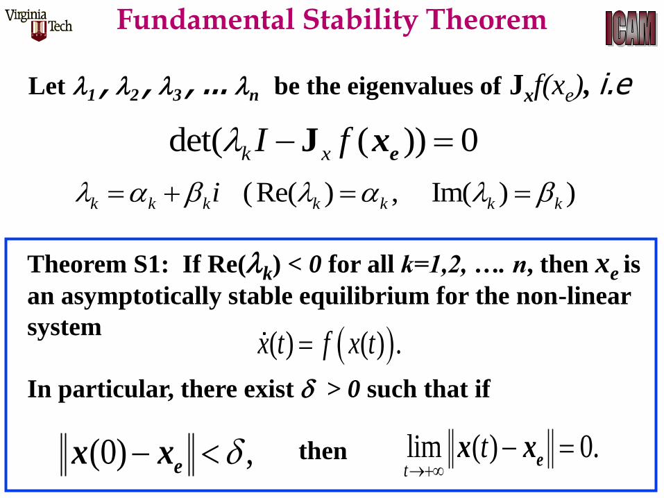
det( ( )) 0k xI f J ex
Let 1 , 2 , 3 , … n be the eigenvalues of Jxf(xe), i.e
(Re( ) , Im( ) )k k k k k k ki
Theorem S1: If Re(k) < 0 for all k=1,2, …. n, then xe is
an asymptotically stable equilibrium for the non-linear
system
In particular, there exist > 0 such that if
then
( ) ( ) .x t f x t
(0) , ex x lim ( ) 0.t
t
ex x
Fundamental Stability Theorem
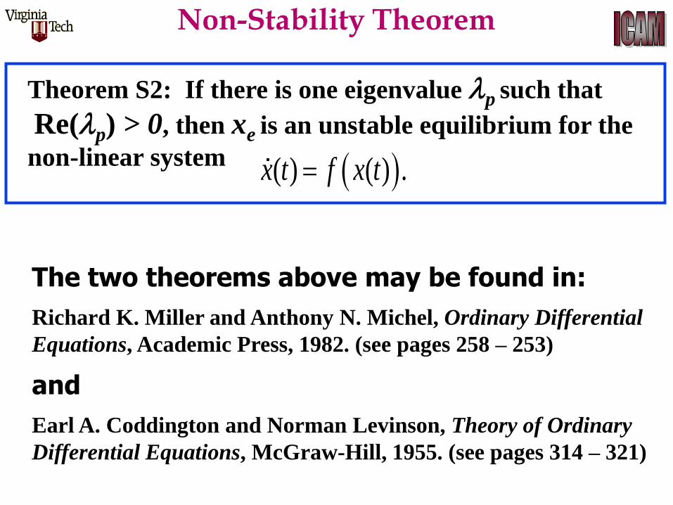
Theorem S2: If there is one eigenvalue p such that
Re(p) > 0, then xe is an unstable equilibrium for the
non-linear system
( ) ( ) .x t f x t
Non-Stability Theorem
The two theorems above may be found in:
Richard K. Miller and Anthony N. Michel, Ordinary Differential
Equations, Academic Press, 1982. (see pages 258 – 253)
and
Earl A. Coddington and Norman Levinson, Theory of Ordinary
Differential Equations, McGraw-Hill, 1955. (see pages 314 – 321)
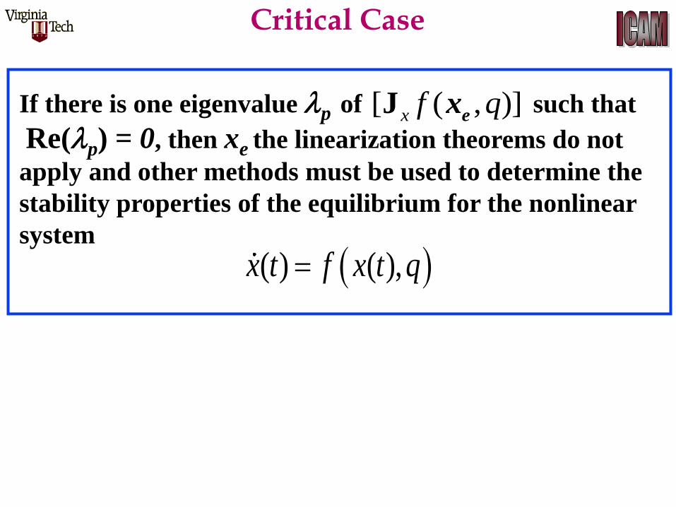
Critical Case
If there is one eigenvalue p of such that
Re(p) = 0, then xe the linearization theorems do not
apply and other methods must be used to determine the
stability properties of the equilibrium for the nonlinear
system
( ) ( ),x t f x t q
[ ( , )]x f qJ ex
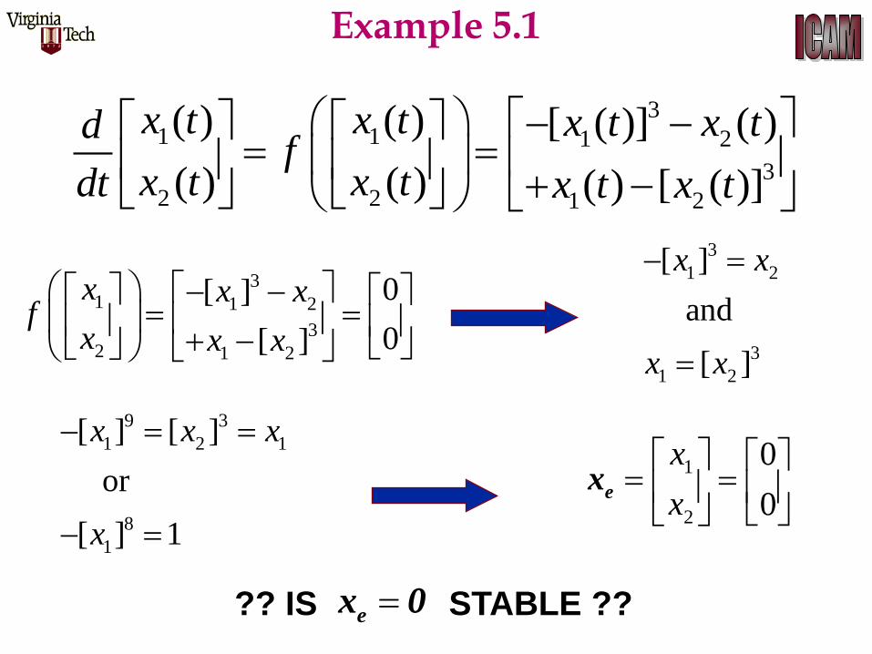
31 1 1 2
32 2 1 2
( ) ( ) [ ( )] ( )
( ) ( ) ( ) [ ( )]
x t x t x t x tdf
x t x tdt x t x t
31 1 2
32 1 2
0[ ]
0[ ]
x x xf
x x x
1
2
0
0
x
x
e
x
?? IS STABLE ?? e
x 0
3
1 2
3
1 2
[ ]
and
[ ]
x x
x x
9 3
1 2 1
8
1
[ ] [ ]
or
[ ] 1
x x x
x
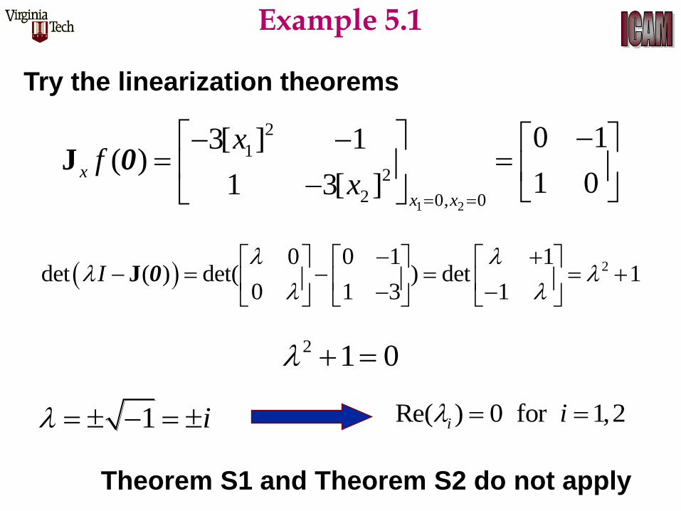
Example 5.1
1 2
2
1
2
2 0, 0
0 13[ ] 1( )
1 01 3[ ]
x
x x
xf
xJ 0
Try the linearization theorems
20 0 1 1
det ( ) det( ) det 10 1 3 1
I
J 0
2 1 0
1 i Re( ) 0 for 1,2i i
Theorem S1 and Theorem S2 do not apply
Example 5.1
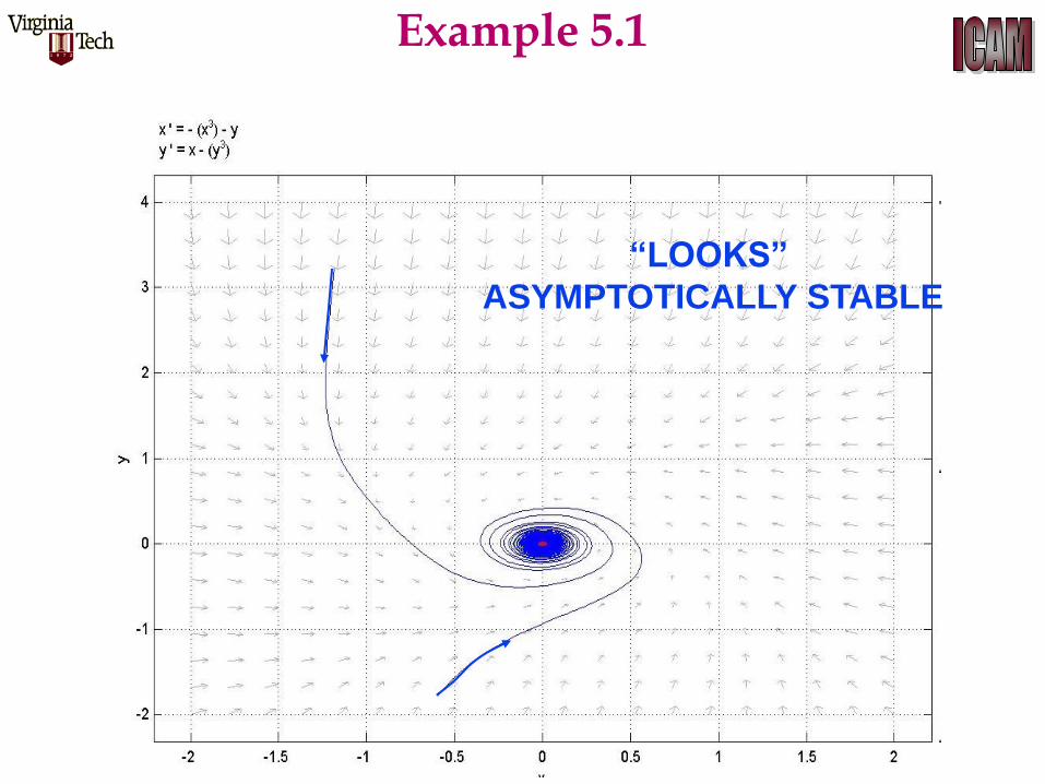
“LOOKS”
ASYMPTOTICALLY STABLE
Example 5.1
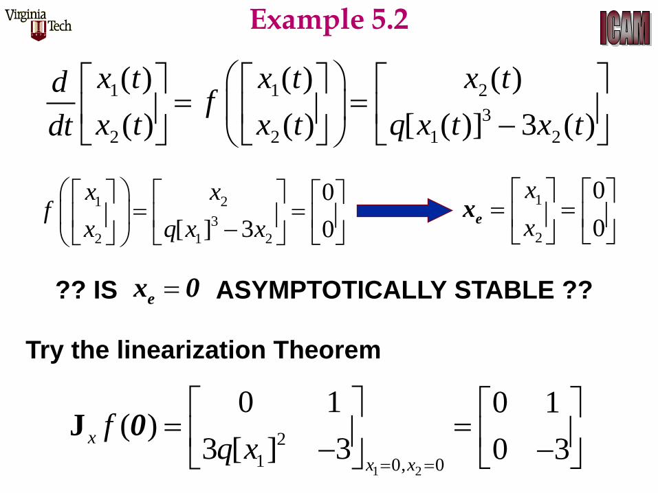
1 1 2
3
2 2 1 2
( ) ( ) ( )
( ) ( ) [ ( )] 3 ( )
x t x t x tdf
x t x t q x t x tdt
1 2
3
2 1 2
0
[ ] 3 0
x xf
x q x x
1
2
0
0
x
x
e
x
1 2
2
1 0, 0
0 1 0 1( )
3 [ ] 3 0 3
x
x x
fq x
J 0
Try the linearization Theorem
?? IS ASYMPTOTICALLY STABLE ?? e
x 0
Example 5.2
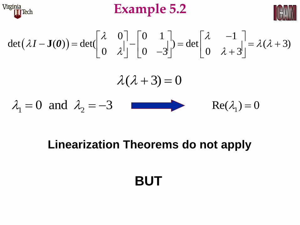
0 0 1 1
det ( ) det( ) det ( 3)0 0 3 0 3
I
J 0
( 3) 0
1 20 and 3 1Re( ) 0
Linearization Theorems do not apply
BUT
Example 5.2
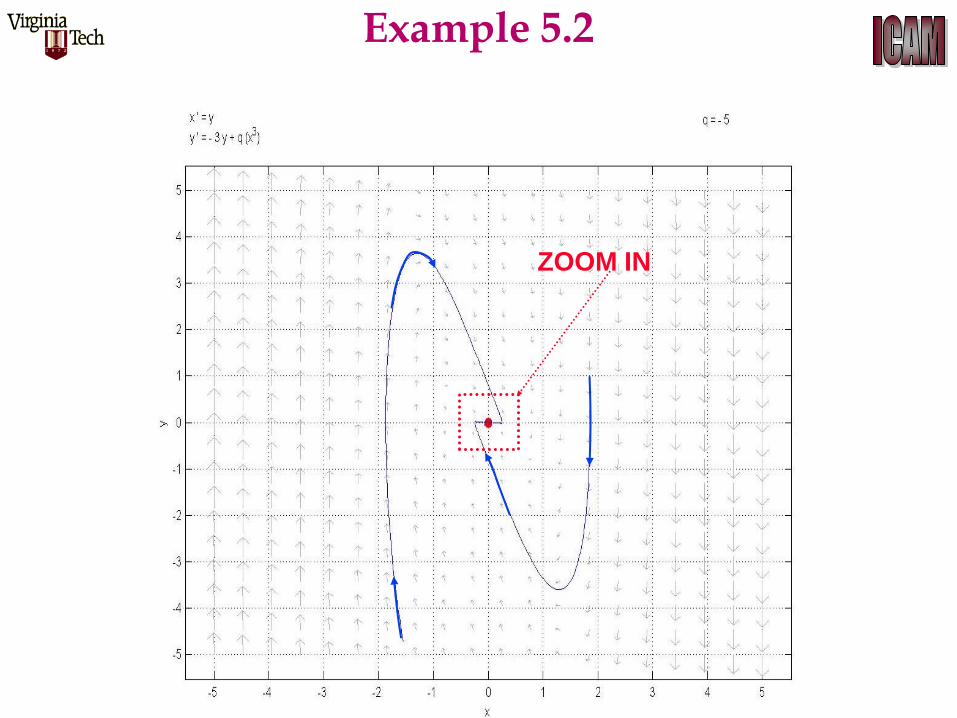
ZOOM IN
Example 5.2
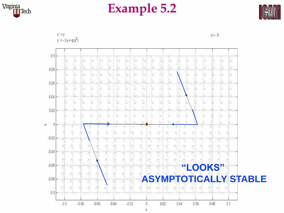
“LOOKS”
ASYMPTOTICALLY STABLE
Example 5.2
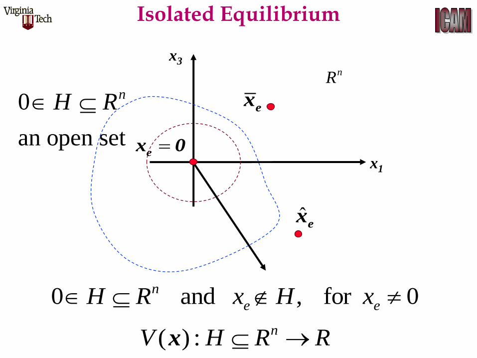
nR
x3
x1
e
x 0
ex
ˆe
x
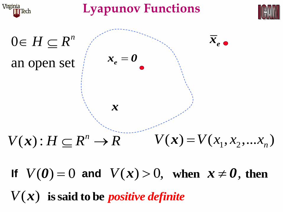
( ) : nV H R R x
0 and , for 0n
e eH R x H x
0
an open set
nH R
Isolated Equilibrium
e
x 0
0
an open set
nH R ex
( ) : nV H R R x
x
1 2( ) ( , ,... )nV V x x xx
If and ( ) 0V 0 ( ) 0, V , when thenx x 0
( ) V is said to be positive definitex
Lyapunov Functions
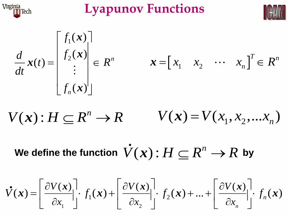
1
2
( )
( )( )
( )
n
n
f
fdt R
dt
f
x
xx
x
We define the function by ( ) : nV H R R x.
1 2
1 2
( ) ( ) ( )( ) ( ) ( ) ... ( )
n
n
V V V
x x xV f f f
x x xx x x x
.
1 2
T n
nx x x R x
( ) : nV H R R x 1 2( ) ( , ,... )nV V x x xx
Lyapunov Functions
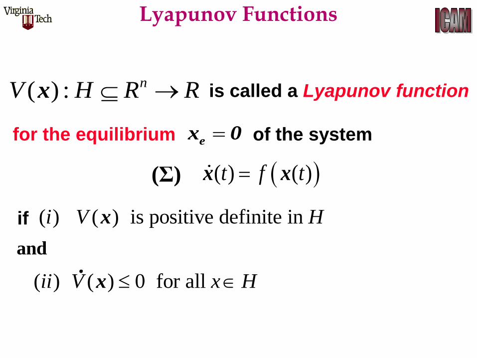
( ) : nV H R R x is called a Lyapunov function
for the equilibrium of the system e
x 0
( ) ( )t f tx x(Σ)
( ) ( ) is positive definite in
( ) ( ) 0 for all
i V H
ii V x H
and
x
x
if
.
Lyapunov Functions
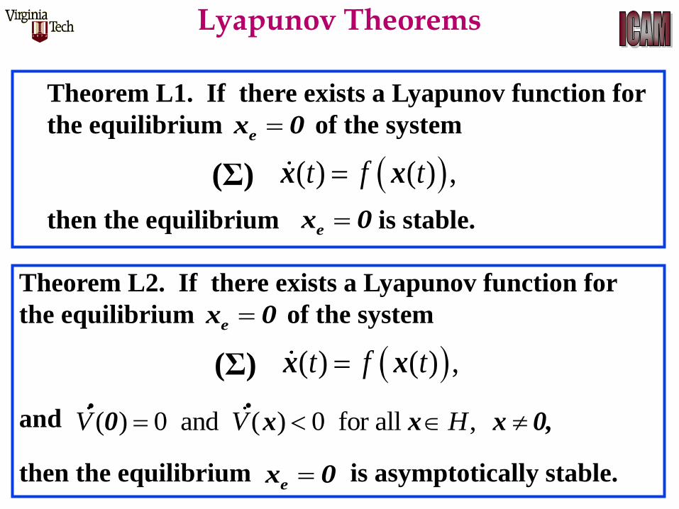
Theorem L1. If there exists a Lyapunov function for
the equilibrium of the system
then the equilibrium is stable.
e
x 0
( ) ( ) ,t f tx x(Σ)
e
x 0
Theorem L2. If there exists a Lyapunov function for
the equilibrium of the system
and
then the equilibrium is asymptotically stable.
e
x 0
( ) ( ) ,t f tx x(Σ)
e
x 0
( ) 0 and ( ) 0 for all , V V H 0 x x x 0,. .
Lyapunov Theorems
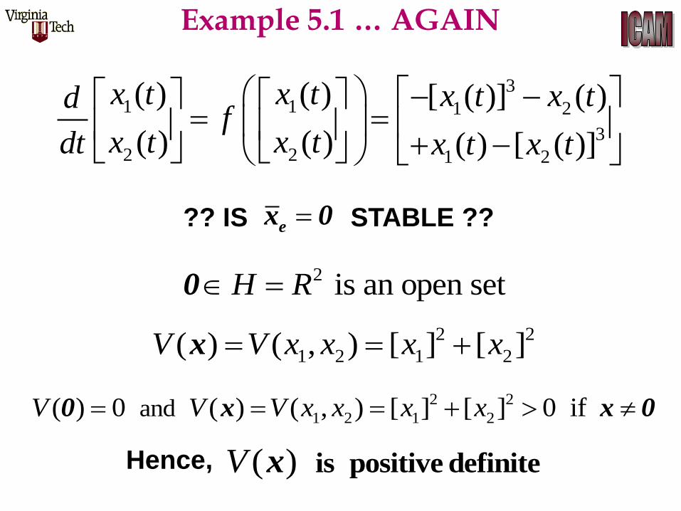
31 1 1 2
32 2 1 2
( ) ( ) [ ( )] ( )
( ) ( ) ( ) [ ( )]
x t x t x t x tdf
x t x tdt x t x t
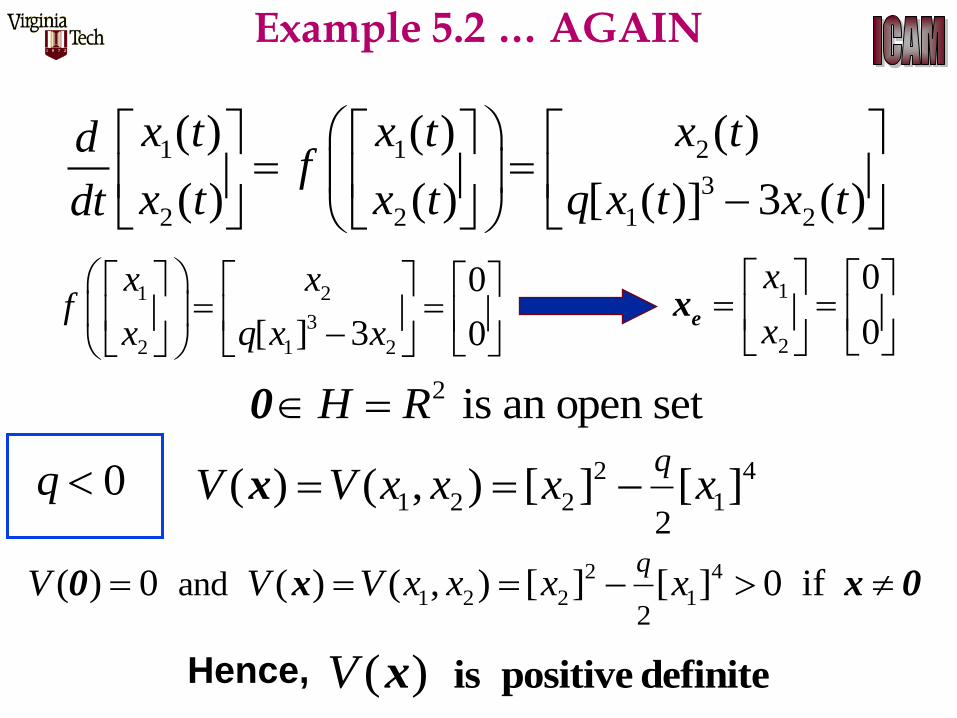
2 2
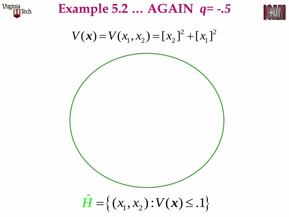
1 2 1 2( ) ( , ) [ ] [ ]V V x x x x x
2 is an open setH R 0
2 2
1 2 1 2and( ) 0 ( ) ( , ) [ ] [ ] 0 if V V V x x x x 0 x x 0
Hence, ( ) V is positive definitex
?? IS STABLE ?? e
x 0
Example 5.1 … AGAIN

1 2 1 2
1 2
1 2 1 1 2 2 1 2
( , ) ( , )( , ) ( , ) ( , )
V x x V x x
x xV x x f x x f x x
.
2 2
1 2 1 2( ) ( , ) [ ] [ ]V V x x x x x
1 21
1
( , )2
V x xx
x
1 22
2
( , )2
V x xx
x
1 2 1 2
1 2
1 2 1 1 2 2 1 2
( , ) ( , )( , ) ( , ) ( , )
V x x V x x
x xV x x f x x f x x
. 12x 22x3
1 2( [ ] )x x 3
1 2( [ ] )x x
31 1 1 2 1 2
32 2 1 2 1 2
( , ) [ ]
( , ) [ ]
x f x x x xf
x f x x x x
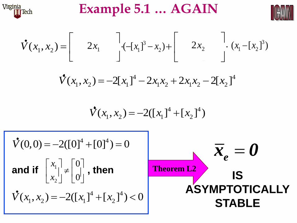
Example 5.1 … AGAIN
1 2 1 2
1 2
1 2 1 1 2 2 1 2
( , ) ( , )( , ) ( , ) ( , )
V x x V x x
x xV x x f x x f x x
. 12x 22x3
1 2( [ ] )x x 3
1 2( [ ] )x x
4 4
1 2 1 1 2 1 2 2( , ) 2[ ] 2 2 2[ ]V x x x x x x x x .
4 4
1 2 1 2( , ) 2([ ] [ ] )V x x x x .
4 4(0,0) 2([0] [0] ) 0V .
4 4
1 2 1 2( , ) 2([ ] [ ] ) 0V x x x x .
1
2
0
0
x
x
and if , then Theorem L2 IS
ASYMPTOTICALLY
STABLE
e
x 0
Example 5.1 … AGAIN

2 4
1 2 2 12
( ) ( , ) [ ] [ ]q
V V x x x x x
2 is an open setH R 0
2 4
1 2 2 12
and( ) 0 ( ) ( , ) [ ] [ ] 0 if q
V V V x x x x 0 x x 0
Hence, ( ) V is positive definitex
1 1 2
3
2 2 1 2
( ) ( ) ( )
( ) ( ) [ ( )] 3 ( )
x t x t x tdf
x t x t q x t x tdt
1 2
3
2 1 2
0
[ ] 3 0
x xf
x q x x
1
2
0
0
x
x
e
x
0q
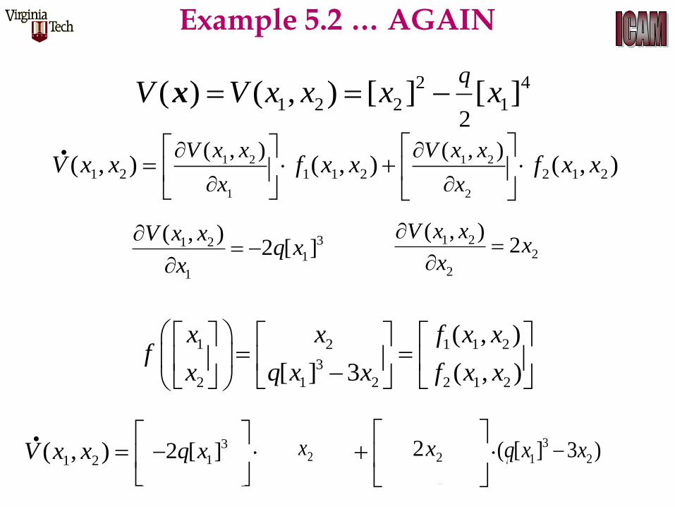
Example 5.2 … AGAIN

1 2 1 1 2
3
2 1 2 2 1 2
( , )
[ ] 3 ( , )
x x f x xf
x q x x f x x
1 2 1 2
1 2
1 2 1 1 2 2 1 2
( , ) ( , )( , ) ( , ) ( , )
V x x V x x
x xV x x f x x f x x
.
31 21
1
( , )2 [ ]
V x xq x
x
1 22
2
( , )2
V x xx
x
1 2 1 2
1 2
1 2 1 1 2 2 1 2
( , ) ( , )( , ) ( , ) ( , )
V x x V x x
x xV x x f x x f x x
. 3
12 [ ]q x 22x2x 3
1 2( [ ] 3 )q x x
2 4
1 2 2 12
( ) ( , ) [ ] [ ]q
V V x x x x x
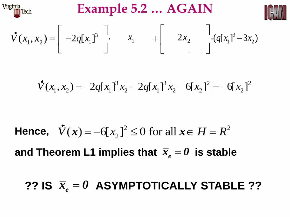
Example 5.2 … AGAIN

3 3 2 2
1 2 1 2 1 2 2 2( , ) 2 [ ] 2 [ ] 6[ ] 6[ ]V x x q x x q x x x x .
1 2 1 2
1 2
1 2 1 1 2 2 1 2
( , ) ( , )( , ) ( , ) ( , )
V x x V x x
x xV x x f x x f x x
. 3
12 [ ]q x 22x2x 3
1 2( [ ] 3 )q x x
e
x 0
Hence, 2 2
2( ) 6[ ] 0 for all V x H R x x.
and Theorem L1 implies that is stable
?? IS ASYMPTOTICALLY STABLE ?? e
x 0
Example 5.2 … AGAIN
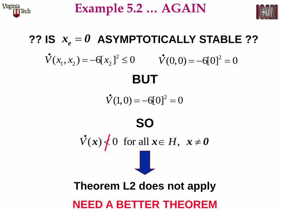
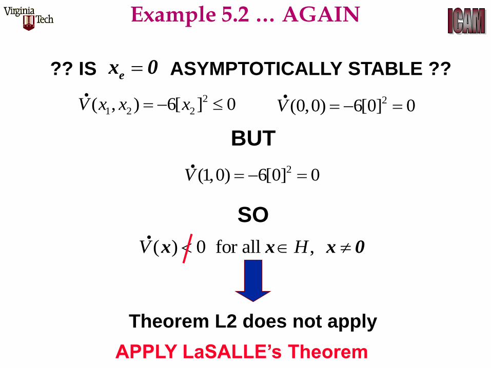
?? IS ASYMPTOTICALLY STABLE ?? e
x 0
2
1 2 2( , ) 6[ ] 0V x x x .
2(0,0) 6[0] 0V .
. 2(1,0) 6[0] 0V
BUT
SO
( ) 0 for all , V H x x x 0.
Theorem L2 does not apply
NEED A BETTER THEOREM
Example 5.2 … AGAIN
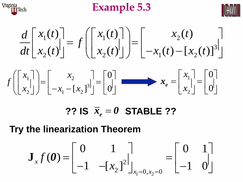
1 1 2
3
2 2 1 2
( ) ( ) ( )
( ) ( ) ( ) [ ( )]
x t x t x tdf
x t x t x t x tdt
1 2
3
2 1 2
0
[ ] 0
x xf
x x x
1
2
0
0
x
x
e
x
1 2
2
2 0, 0
0 1 0 1( )
1 [ ] 1 0x
x x
fx
J 0
Try the linearization Theorem
?? IS STABLE ?? e
x 0
Example 5.3
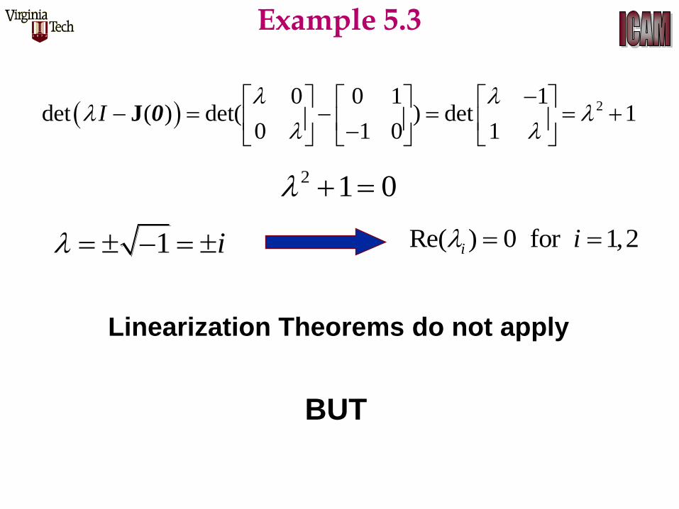
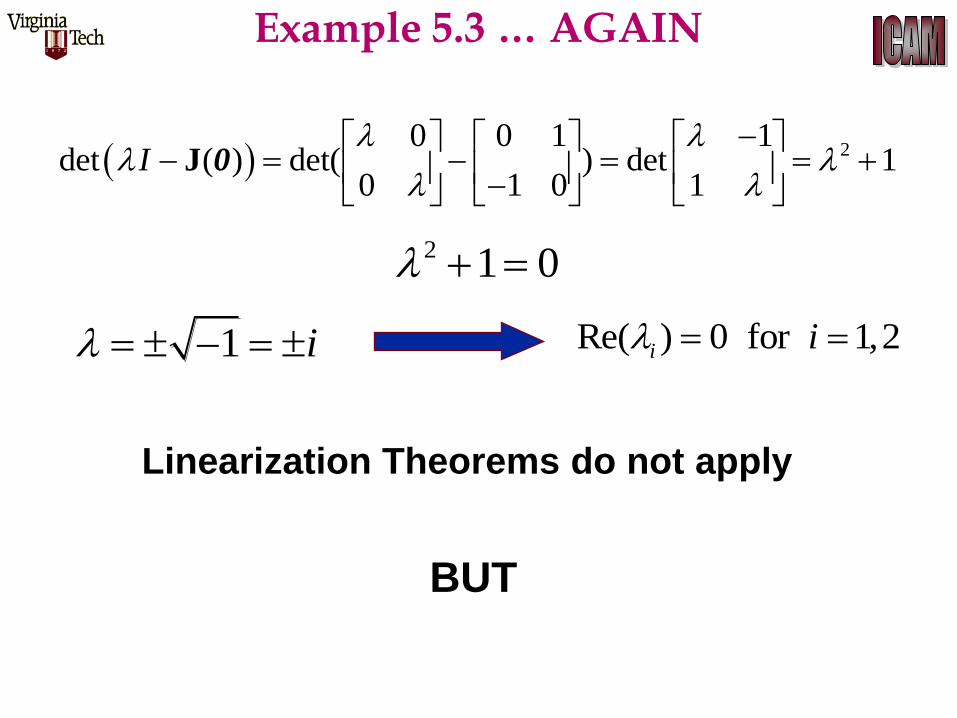
20 0 1 1
det ( ) det( ) det 10 1 0 1
I
J 0
2 1 0
1 i Re( ) 0 for 1,2i i
Linearization Theorems do not apply
BUT
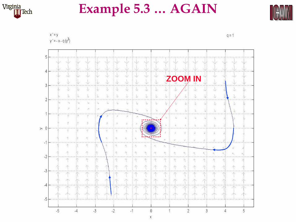
Example 5.3
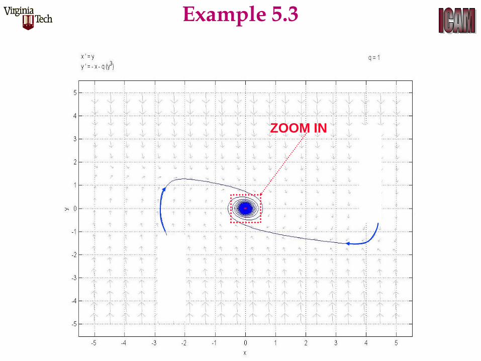
ZOOM IN
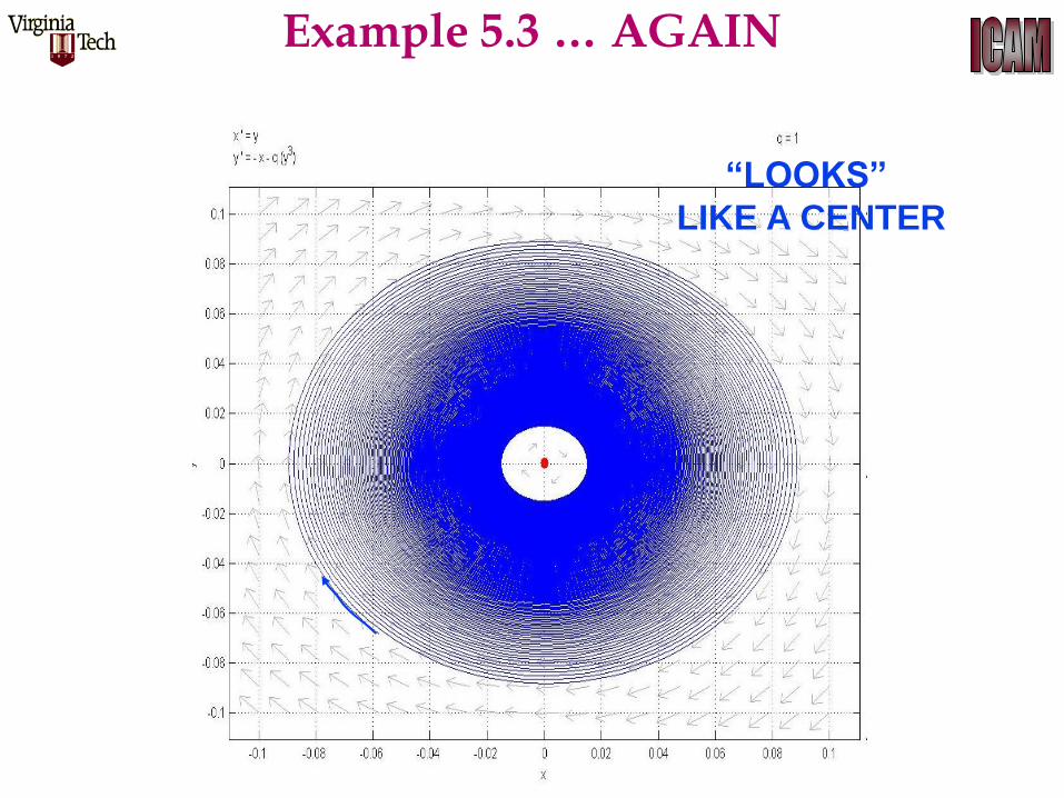
Example 5.3
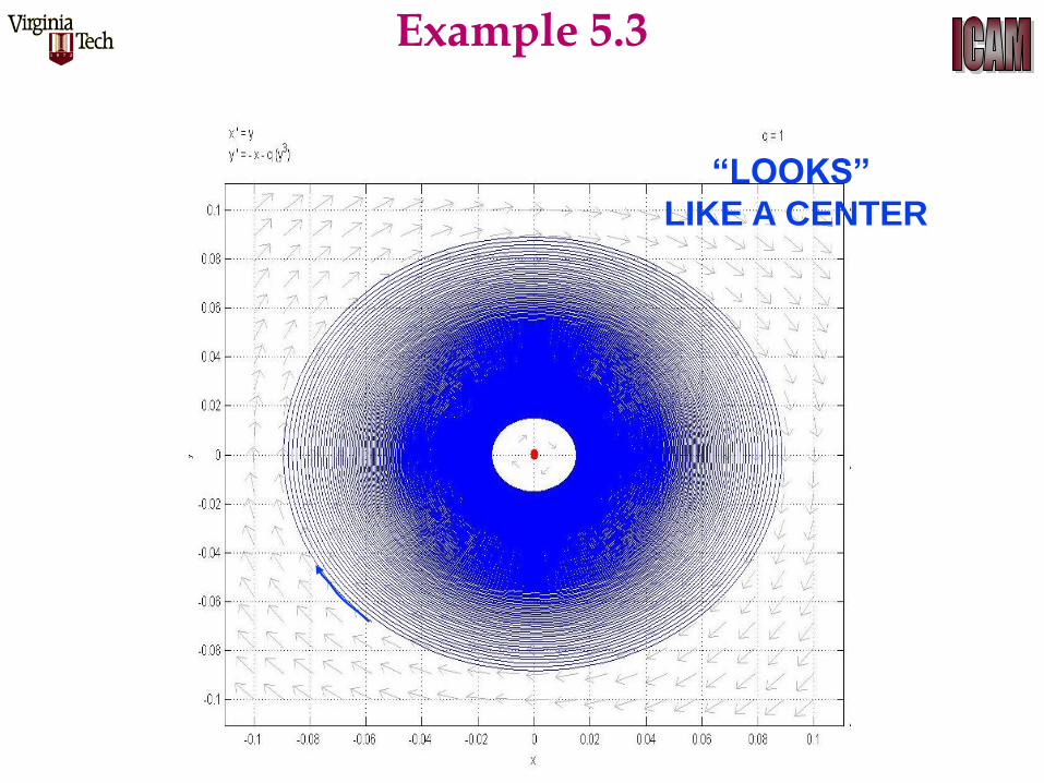
“LOOKS”
LIKE A CENTER
Example 5.3
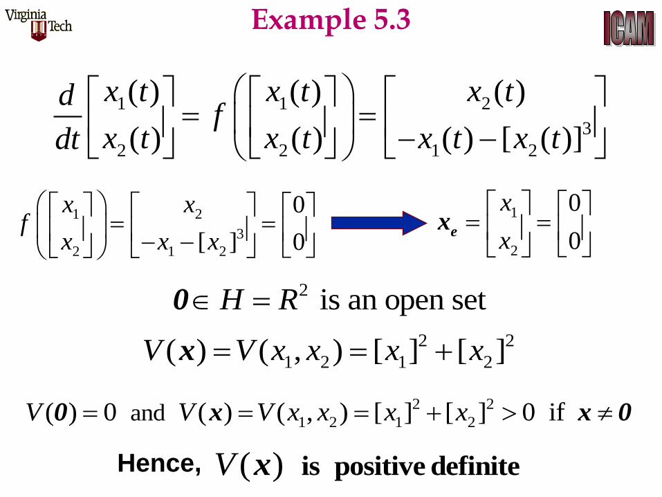
1 1 2
3
2 2 1 2
( ) ( ) ( )
( ) ( ) ( ) [ ( )]
x t x t x tdf
x t x t x t x tdt
2 2
1 2 1 2( ) ( , ) [ ] [ ]V V x x x x x
1 2
3
2 1 2
0
[ ] 0
x xf
x x x
1
2
0
0
x
x
e
x
2 is an open setH R 0
2 2
1 2 1 2and( ) 0 ( ) ( , ) [ ] [ ] 0 if V V V x x x x 0 x x 0
Hence, ( ) V is positive definitex
Example 5.3
1 2 1 1 2
3
2 1 2 2 1 2
( , )
[ ] ( , )
x x f x xf
x x x f x x
1 2 1 2
1 2
1 2 1 1 2 2 1 2
( , ) ( , )( , ) ( , ) ( , )
V x x V x x
x xV x x f x x f x x
.
2 2
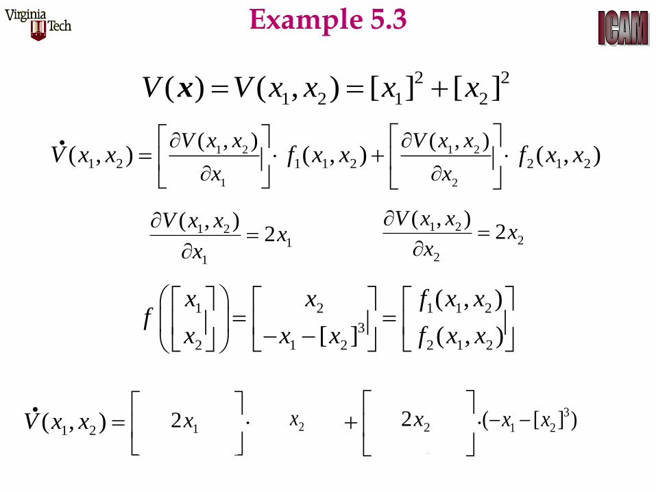
1 2 1 2( ) ( , ) [ ] [ ]V V x x x x x
1 21
1
( , )2
V x xx
x
1 22
2
( , )2
V x xx
x
1 2 1 2
1 2
1 2 1 1 2 2 1 2
( , ) ( , )( , ) ( , ) ( , )
V x x V x x
x xV x x f x x f x x
. 12x 22x2x 3
1 2( [ ] )x x
Example 5.3
1 2 1 2
1 2
1 2 1 1 2 2 1 2
( , ) ( , )( , ) ( , ) ( , )
V x x V x x
x xV x x f x x f x x
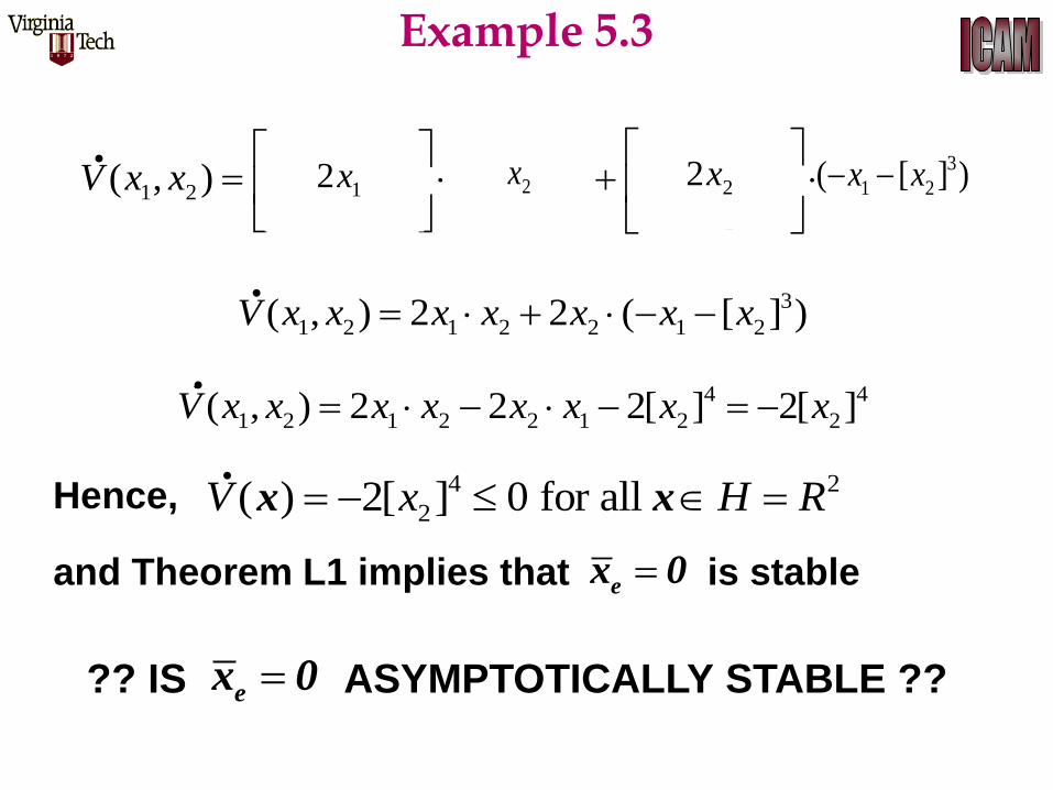
. 12x 22x2x 3
1 2( [ ] )x x
3
1 2 1 2 2 1 2( , ) 2 2 ( [ ] )V x x x x x x x .
4 4
1 2 1 2 2 1 2 2( , ) 2 2 2[ ] 2[ ]V x x x x x x x x .
4 2
2( ) 2[ ] 0 for all V x H R x x.
e
x 0
Hence,
and Theorem L1 implies that is stable
?? IS ASYMPTOTICALLY STABLE ?? e
x 0
Example 5.3
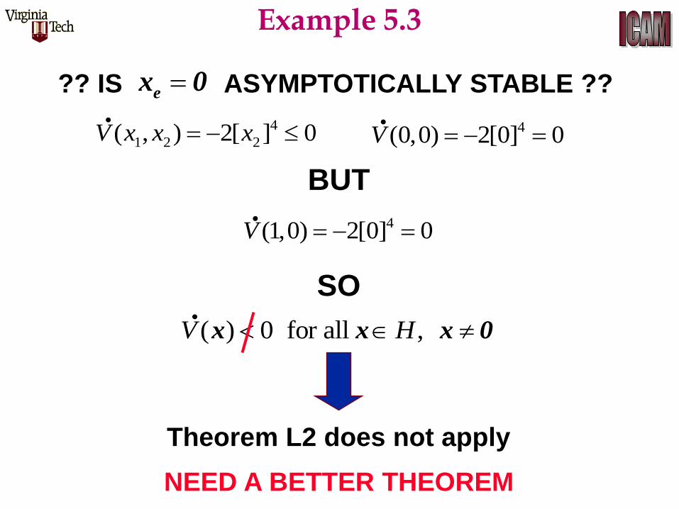
?? IS ASYMPTOTICALLY STABLE ?? e
x 0
4
1 2 2( , ) 2[ ] 0V x x x .
4(0,0) 2[0] 0V .
. 4(1,0) 2[0] 0V
BUT
SO
( ) 0 for all , V H x x x 0.
Theorem L2 does not apply
NEED A BETTER THEOREM
Example 5.3
nR
x3
x1
M
0x
0x
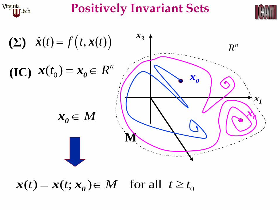
0( ) ( ; ) for all t t M t t 0
x x x
M0
x
0( ) nt R 0x x(IC)
( ) , ( )t f t tx x(Σ)
Positively Invariant Sets
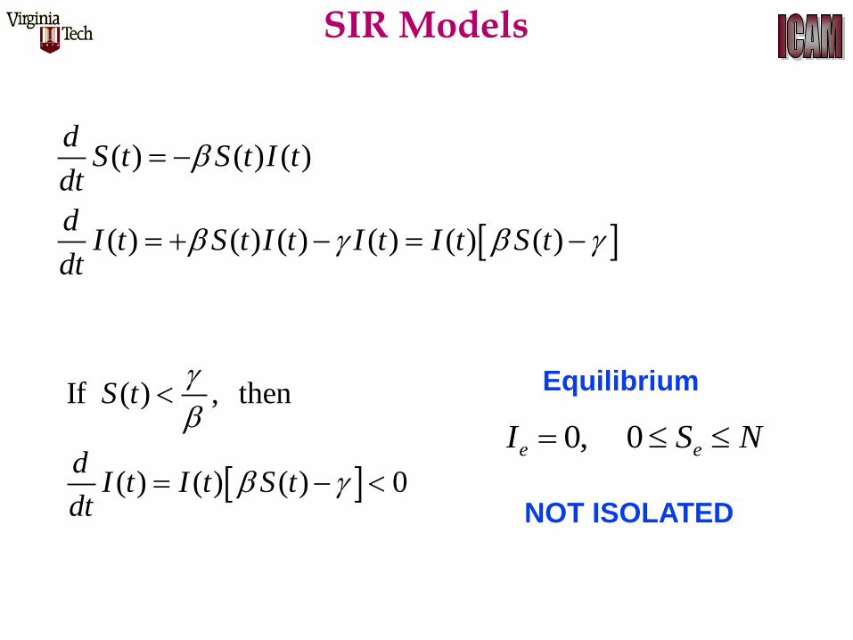
( ) ( ) ( )
( ) ( ) ( ) ( ) ( ) ( )
dS t S t I t
dt
dI t S t I t I t I t S t
dt
If ( ) , then
( ) ( ) ( ) 0
S t
dI t I t S t
dt
NOT ISOLATED
NSI ee 0 ,0
Equilibrium
SIR Models
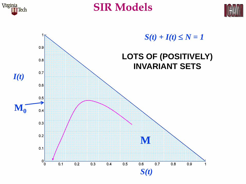
I(t)
S(t)
S(t) + I(t) N = 1
M
M0
LOTS OF (POSITIVELY)
INVARIANT SETS
SIR Models
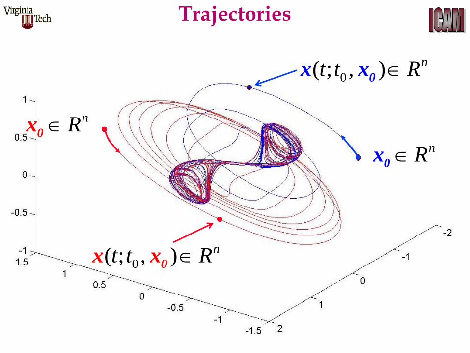
0( ; , ) nt t R0x x
0( ; , ) nt t R0x x
nR0x
nR0x
Trajectories
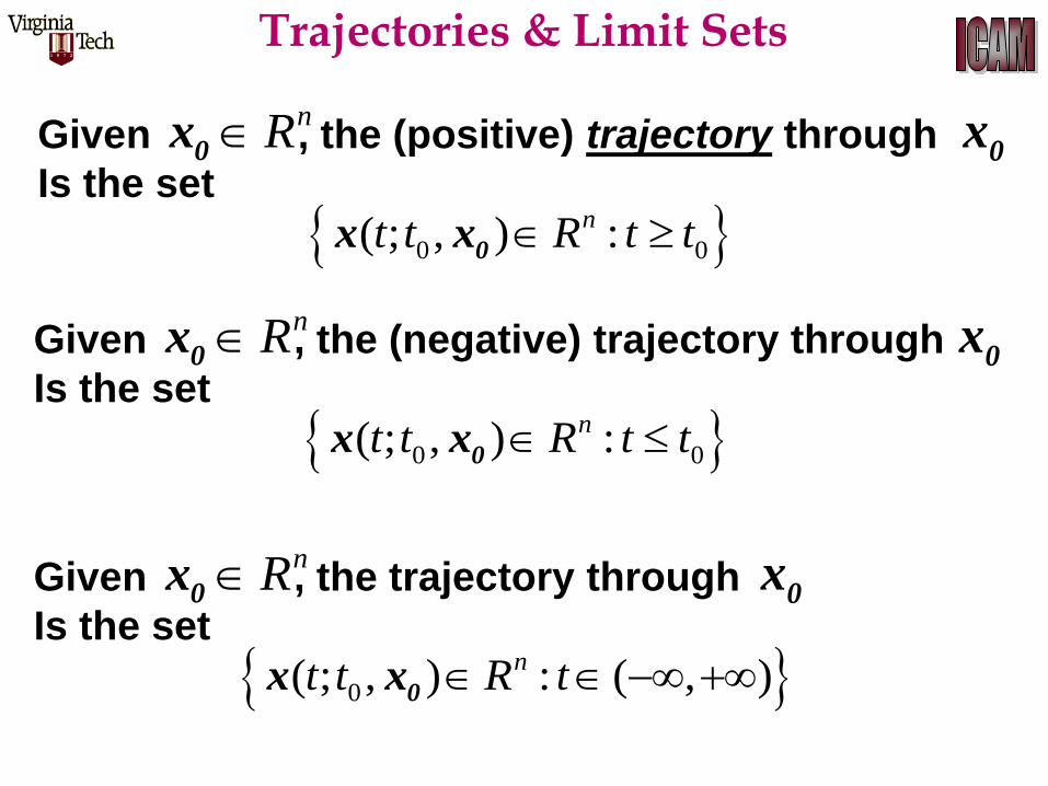
Given , the (positive) trajectory through
Is the set
nR0x 0x
0 0( ; , ) :nt t R t t 0x x
Given , the (negative) trajectory through
Is the set
nR0x 0x
0 0( ; , ) :nt t R t t 0x x
Given , the trajectory through
Is the set
nR0x 0x
0( ; , ) : ( , )nt t R t 0x x
Trajectories & Limit Sets
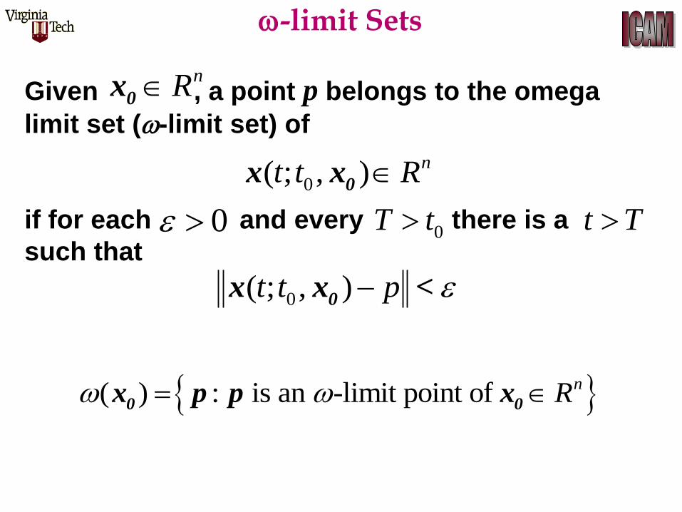
Given , a point p belongs to the omega
limit set (-limit set) of
if for each and every there is a
such that
nR0x
0( ; , ) nt t R0x x
0 0T t t T
0( ; , )t t p 0x x <
( ) : is an -limit point of nR 0 0x p p x
-limit Sets
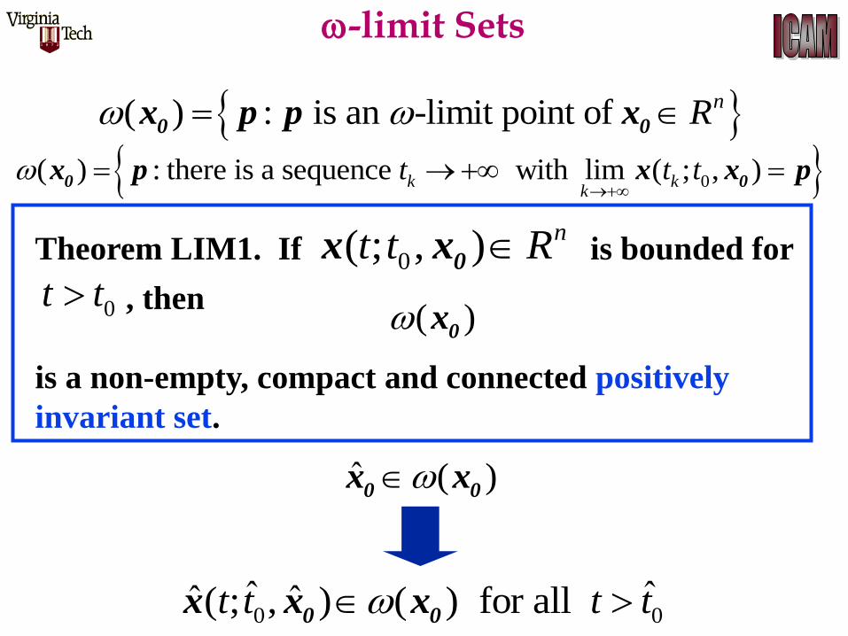
( ) : is an -limit point of nR 0 0x p p x
0( ) : there is a sequence with lim ( ; , )k kk
t t t
0 0x p x x p
Theorem LIM1. If is bounded for
, then
is a non-empty, compact and connected positively
invariant set.
0( ; , ) nt t R0x x
0t t( ) 0x
0 0ˆ ˆˆ ˆ( ; , ) ( ) for all t t t t 0 0x x x
ˆ ( )0 0x x
-limit Sets

nR
x3
x1
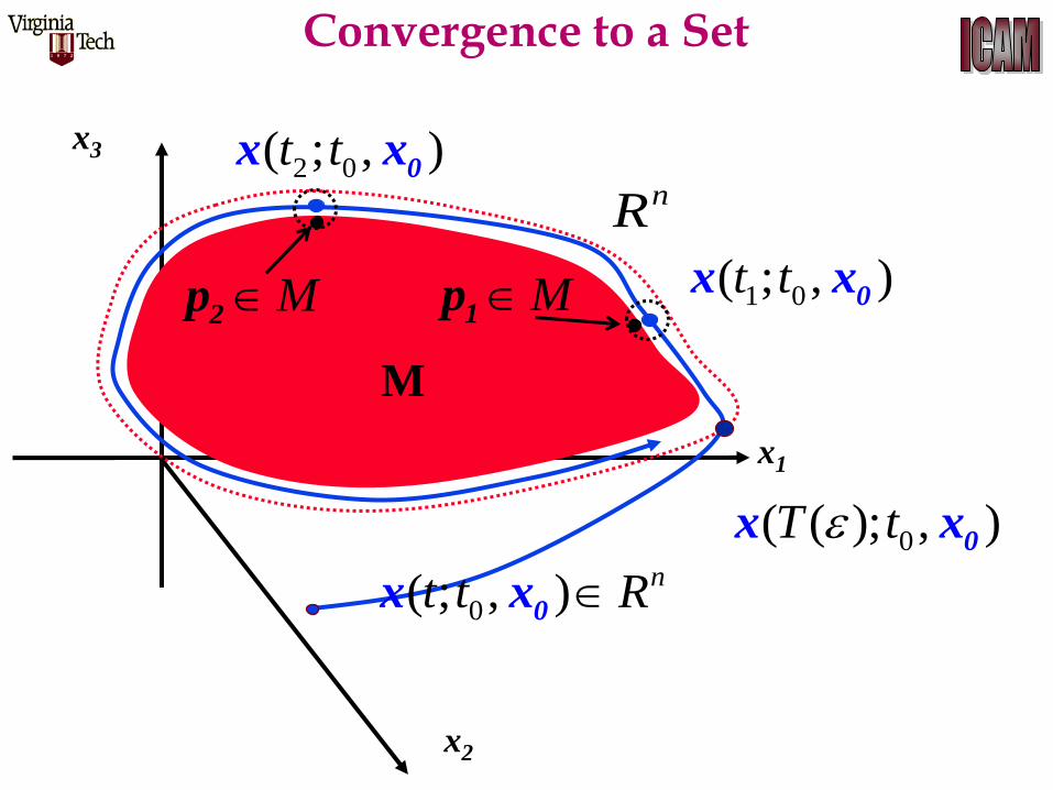
( ) ( ; )
as
t t M
t
0x x x
M
0
For any 0 there is a
( ) such that
if ( ), then there is
a point with
( ; )
T T t
t T
p M
t p
0x x <
Convergence to a Set
nR
x3
x1
x2
M
0( ; , ) nt t R0x x
1 0( ; , )t t 0x xM1p
0( ( ); , )T t 0x x
2 0( ; , )t t 0x x
M2p
Convergence to a Set
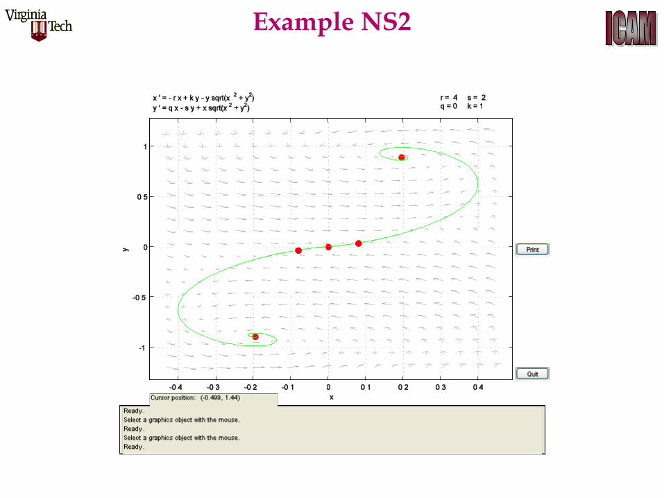
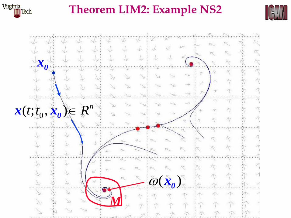
Example NS2
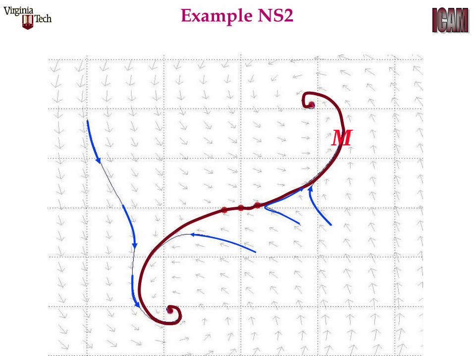
M
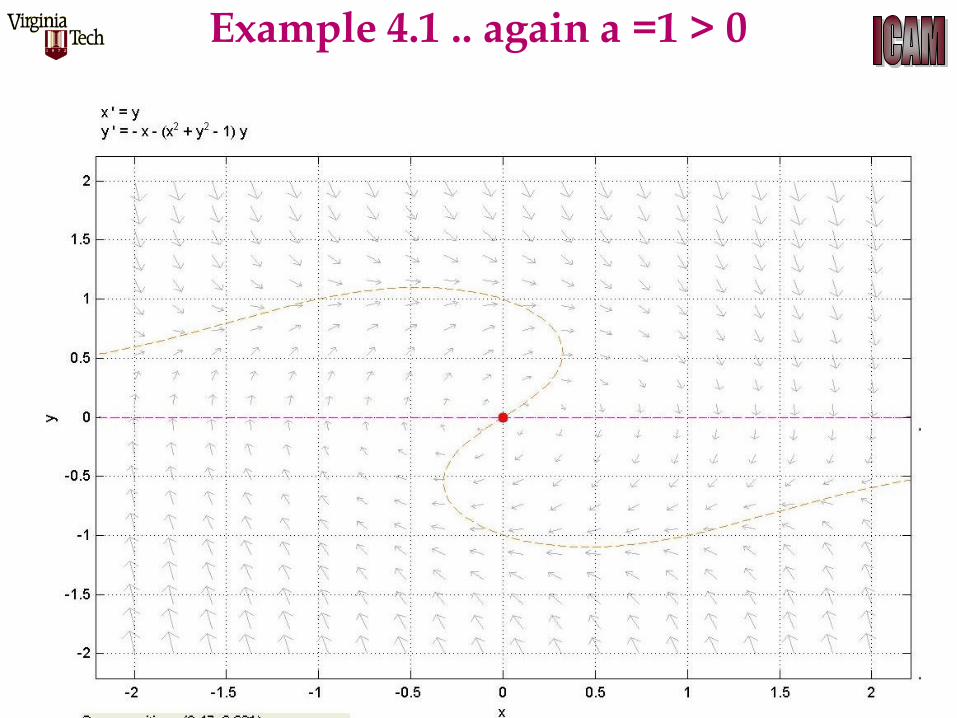
Example NS2
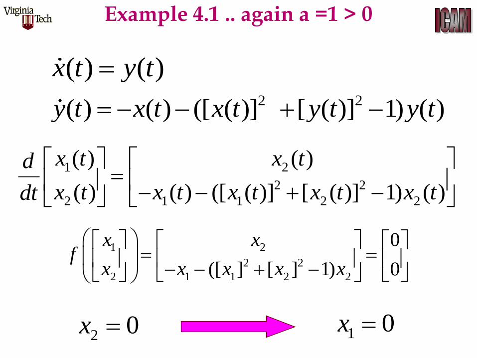
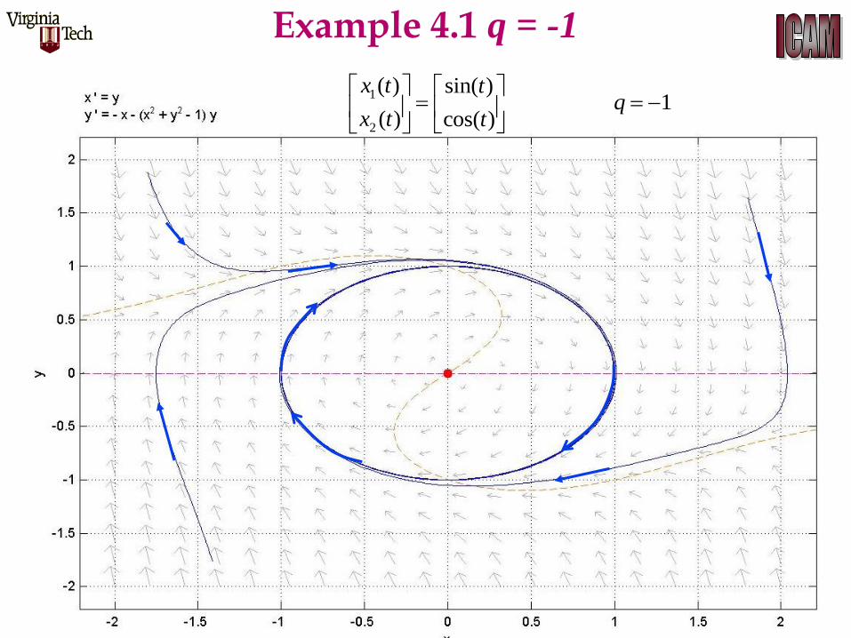
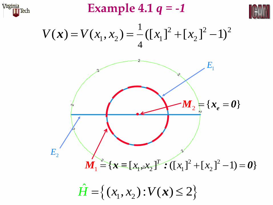
( ) ( )x t y t2 2( ) ( ) ([ ( )] [ ( )] 1) ( )y t x t x t y t y t
1 2
2 2
2 1 1 2 2
( ) ( )
( ) ( ) ([ ( )] [ ( )] 1) ( )
x t x td
x t x t x t x t x tdt
1 2
2 2
2 1 1 2 2
0
([ ] [ ] 1) 0
x xf
x x x x x
2 0x 1 0x
Example 4.1 .. again a =1 > 0
Example 4.1 .. again a =1 > 0
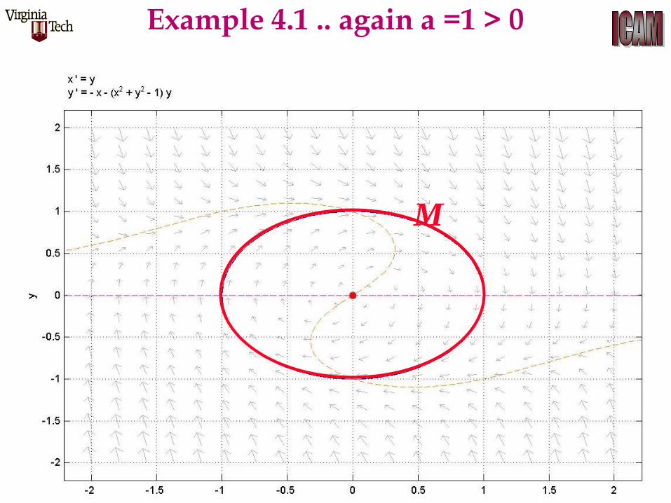
M
Example 4.1 .. again a =1 > 0
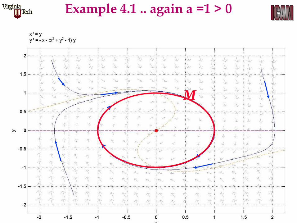
M
Example 4.1 .. again a =1 > 0
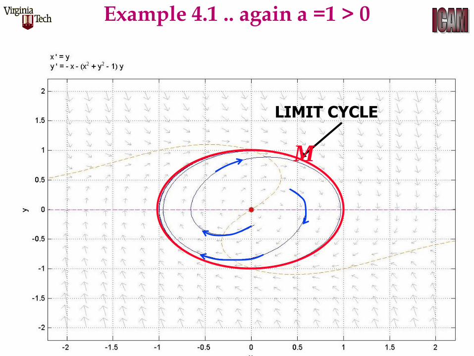
LIMIT CYCLE
M
Example 4.1 .. again a =1 > 0
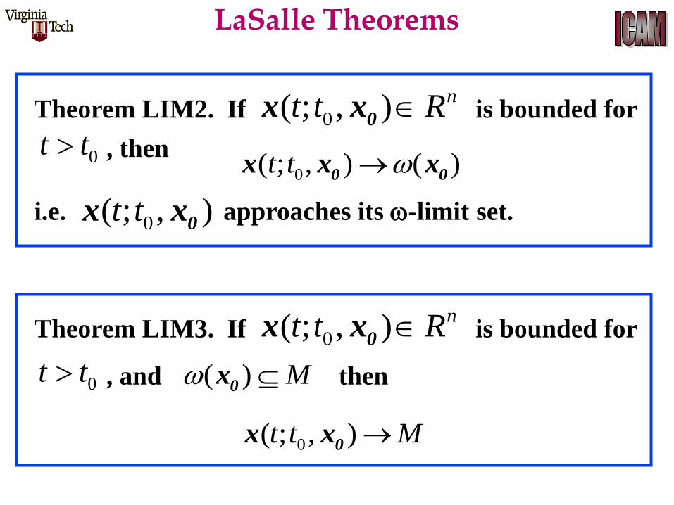
Theorem LIM2. If is bounded for
, then
i.e. approaches its -limit set.
0( ; , ) nt t R0x x
0t t0( ; , ) ( )t t 0 0x x x
0( ; , )t t 0x x
Theorem LIM3. If is bounded for
, and then
0( ; , ) nt t R0x x
0t t ( ) M 0x
0( ; , )t t M0x x
LaSalle Theorems
0( ; , ) nt t R0x x
( ) 0x
0x
M
Theorem LIM2: Example NS2
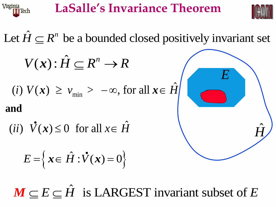
ˆLet be a bounded closed positively invariant setnH R
H
ˆ( ) : nV H R R x
minˆ ( ) ( ) > , for all
ˆ ( ) ( ) 0 for all
i V v H
ii V x H
and
x x
x.
ˆ : ( ) 0E H V x x.
E
ˆ is LARGEST invariant subset of E H E M
LaSalle’s Invariance Theorem
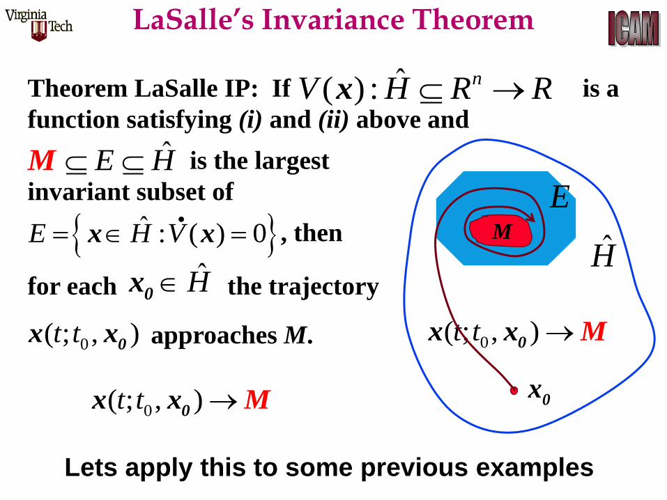
0( ; , )t t 0x x M
Theorem LaSalle IP: If is a
function satisfying (i) and (ii) above and
is the largest
invariant subset of
, then
for each the trajectory
approaches M.
H0x
ˆ( ) : nV H R R x
ˆE H M
ˆ : ( ) 0E H V x x.
0( ; , )t t 0x x
H
0x
EM
Lets apply this to some previous examples
0( ; , )t t 0x x M
LaSalle’s Invariance Theorem
2 4
1 2 2 12
( ) ( , ) [ ] [ ]q
V V x x x x x
2 is an open setH R 0
2 4
1 2 2 12
and( ) 0 ( ) ( , ) [ ] [ ] 0 if q
V V V x x x x 0 x x 0
Hence, ( ) V is positive definitex
1 1 2
3
2 2 1 2
( ) ( ) ( )
( ) ( ) [ ( )] 3 ( )
x t x t x tdf
x t x t q x t x tdt
1 2
3
2 1 2
0
[ ] 3 0
x xf
x q x x
1
2
0
0
x
x
e
x
0q
Example 5.2 … AGAIN
1 2 1 1 2
3
2 1 2 2 1 2
( , )
[ ] 3 ( , )
x x f x xf
x q x x f x x
1 2 1 2
1 2
1 2 1 1 2 2 1 2
( , ) ( , )( , ) ( , ) ( , )
V x x V x x
x xV x x f x x f x x
.
31 21
1
( , )2 [ ]
V x xq x
x
1 22
2
( , )2
V x xx
x
1 2 1 2
1 2
1 2 1 1 2 2 1 2
( , ) ( , )( , ) ( , ) ( , )
V x x V x x
x xV x x f x x f x x
. 3
12 [ ]q x 22x2x 3
1 2( [ ] 3 )q x x
2 4
1 2 2 12
( ) ( , ) [ ] [ ]q
V V x x x x x
Example 5.2 … AGAIN
3 3 2 2
1 2 1 2 1 2 2 2( , ) 2 [ ] 2 [ ] 6[ ] 6[ ]V x x q x x q x x x x .
1 2 1 2
1 2
1 2 1 1 2 2 1 2
( , ) ( , )( , ) ( , ) ( , )
V x x V x x
x xV x x f x x f x x
. 3
12 [ ]q x 22x2x 3
1 2( [ ] 3 )q x x
e
x 0
Hence, 2 2
2( ) 6[ ] 0 for all V x H R x x.
and Theorem L1 implies that is stable
?? IS ASYMPTOTICALLY STABLE ?? e
x 0
Example 5.2 … AGAIN
?? IS ASYMPTOTICALLY STABLE ?? e
x 0
2
1 2 2( , ) 6[ ] 0V x x x .
2(0,0) 6[0] 0V .
. 2(1,0) 6[0] 0V
BUT
SO
( ) 0 for all , V H x x x 0.
Theorem L2 does not apply
APPLY LaSALLE’s Theorem
Example 5.2 … AGAIN
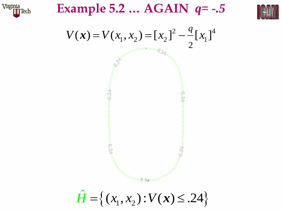
1 2( , ) : ( ) 2ˆ . 4 x x VH x
2 4
1 2 2 12
( ) ( , ) [ ] [ ]q
V V x x x x x
Example 5.2 … AGAIN q= -.5
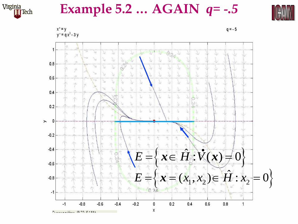
Example 5.2 … AGAIN q= -.5
ˆ : ( ) 0E H V x x.
1 2 2ˆ( , ) : 0 E x x H xx
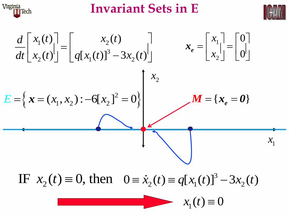
1 2
3
2 1 2
( ) ( )
( ) [ ( )] 3 ( )
x t x td
x t q x t x tdt
1x
2x
2
1 2 2( , ) : 6[ ] 0x x xE x { } e
M x 0
2IF ( ) 0, thenx t 3
2 1 20 ( ) [ ( )] 3 ( )x t q x t x t
1( ) 0x t
1
2
0
0
x
x
e
x
Invariant Sets in E
1x
2x
2
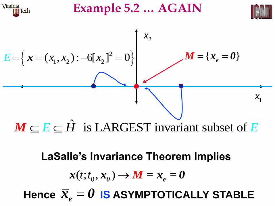
1 2 2( , ) : 6[ ] 0x x xE x { } e
M x 0
ˆ is LARGEST invariant subset of E EH M
0( ; , )t t 0 ex x M = x = 0
LaSalle’s Invariance Theorem Implies
Hence IS ASYMPTOTICALLY STABLE e
x 0
Example 5.2 … AGAIN
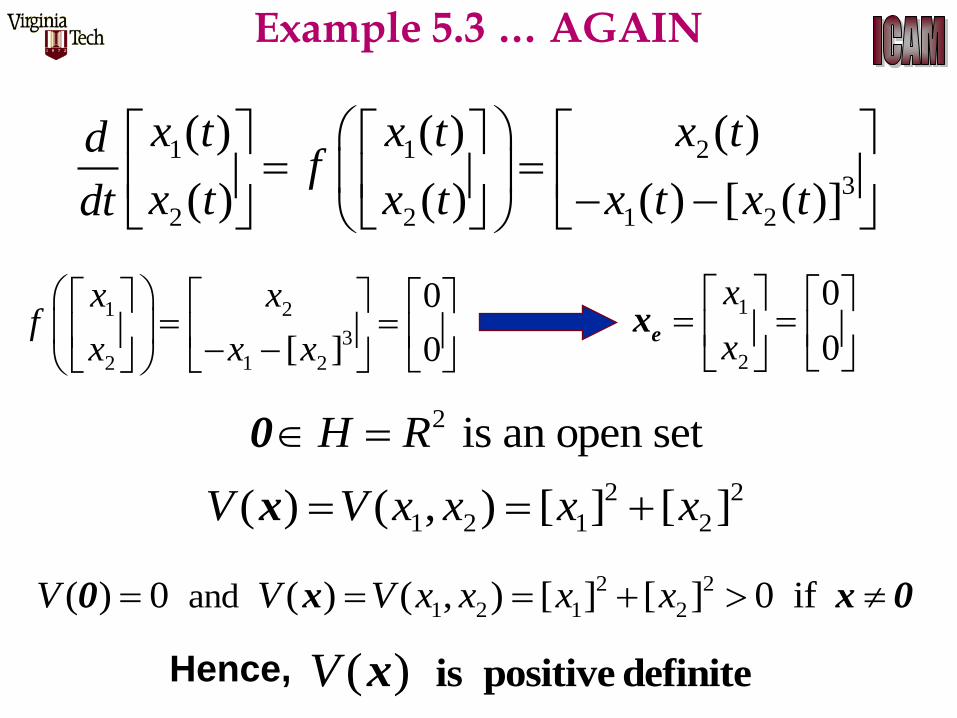
1 1 2
3
2 2 1 2
( ) ( ) ( )
( ) ( ) ( ) [ ( )]
x t x t x tdf
x t x t x t x tdt
1 2
3
2 1 2
0
[ ] 0
x xf
x x x
1
2
0
0
x
x
e
x
1 2
2
2 0, 0
0 1 0 1( )
1 [ ] 1 0x
x x
fx
J 0
Try the linearization Theorem
?? IS STABLE ?? e
x 0
Example 5.3 … AGAIN
20 0 1 1
det ( ) det( ) det 10 1 0 1
I
J 0
2 1 0
1 i Re( ) 0 for 1,2i i
Linearization Theorems do not apply
BUT
Example 5.3 … AGAIN
ZOOM IN
Example 5.3 … AGAIN
“LOOKS”
LIKE A CENTER
Example 5.3 … AGAIN
1 1 2
3
2 2 1 2
( ) ( ) ( )
( ) ( ) ( ) [ ( )]
x t x t x tdf
x t x t x t x tdt
2 2
1 2 1 2( ) ( , ) [ ] [ ]V V x x x x x
1 2
3
2 1 2
0
[ ] 0
x xf
x x x
1
2
0
0
x
x
e
x
2 is an open setH R 0
2 2
1 2 1 2and( ) 0 ( ) ( , ) [ ] [ ] 0 if V V V x x x x 0 x x 0
Hence, ( ) V is positive definitex
Example 5.3 … AGAIN
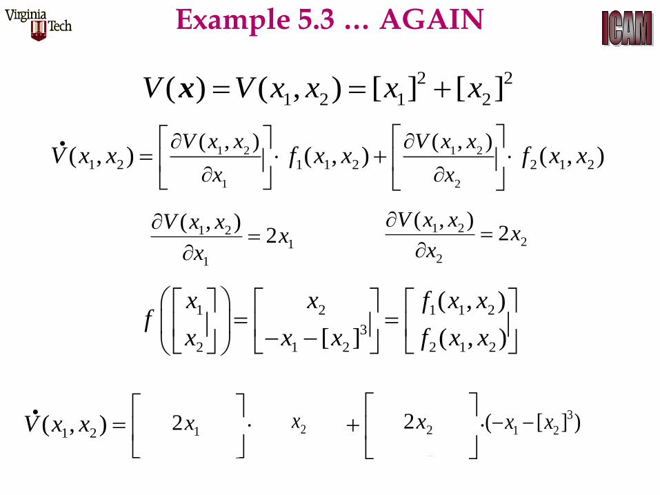
1 2 1 1 2
3
2 1 2 2 1 2
( , )
[ ] ( , )
x x f x xf
x x x f x x
1 2 1 2
1 2
1 2 1 1 2 2 1 2
( , ) ( , )( , ) ( , ) ( , )
V x x V x x
x xV x x f x x f x x
.
2 2
1 2 1 2( ) ( , ) [ ] [ ]V V x x x x x
1 21
1
( , )2
V x xx
x
1 22
2
( , )2
V x xx
x
1 2 1 2
1 2
1 2 1 1 2 2 1 2
( , ) ( , )( , ) ( , ) ( , )
V x x V x x
x xV x x f x x f x x
. 12x 22x2x 3
1 2( [ ] )x x
Example 5.3 … AGAIN
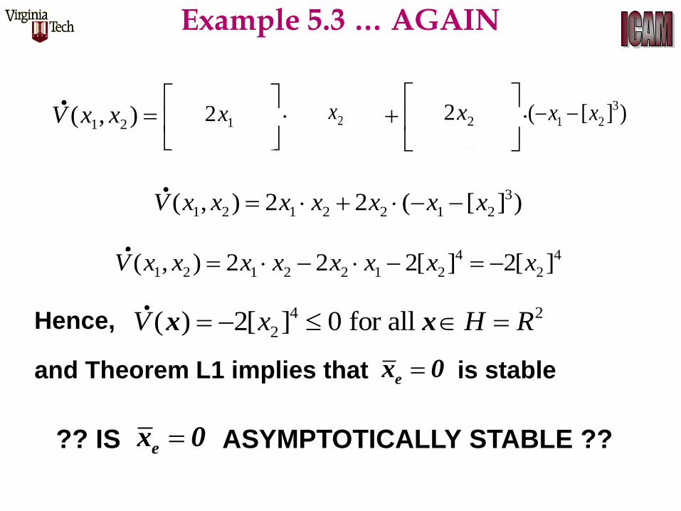
1 2 1 2
1 2
1 2 1 1 2 2 1 2
( , ) ( , )( , ) ( , ) ( , )
V x x V x x
x xV x x f x x f x x
. 12x 22x2x 3
1 2( [ ] )x x
3
1 2 1 2 2 1 2( , ) 2 2 ( [ ] )V x x x x x x x .
4 4
1 2 1 2 2 1 2 2( , ) 2 2 2[ ] 2[ ]V x x x x x x x x .
e
x 0
Hence, 4 2
2( ) 2[ ] 0 for all V x H R x x.
and Theorem L1 implies that is stable
?? IS ASYMPTOTICALLY STABLE ?? e
x 0
Example 5.3 … AGAIN
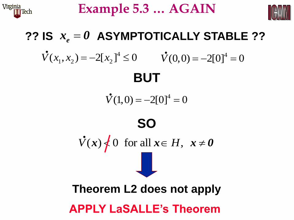
?? IS ASYMPTOTICALLY STABLE ?? e
x 0
4
1 2 2( , ) 2[ ] 0V x x x .
4(0,0) 2[0] 0V .
. 4(1,0) 2[0] 0V
BUT
SO
( ) 0 for all , V H x x x 0.
Theorem L2 does not apply
APPLY LaSALLE’s Theorem
Example 5.3 … AGAIN
1 2( , ) : ( ) 1ˆ . x x VH x
2 2
1 2 2 1( ) ( , ) [ ] [ ] V V x x x xx
Example 5.2 … AGAIN q= -.5
H
4
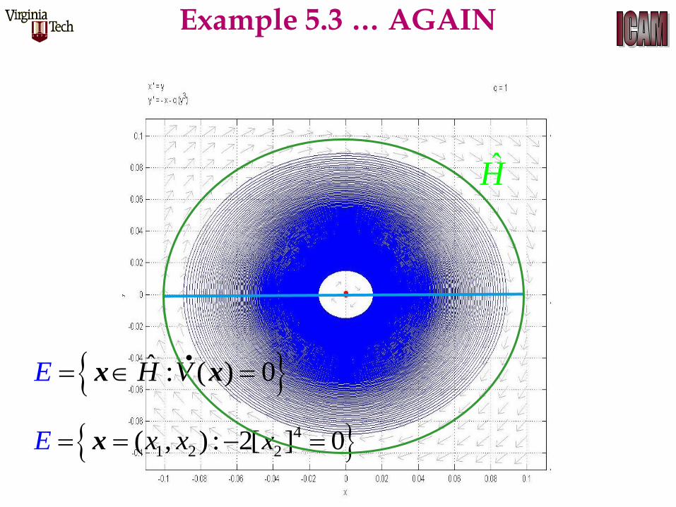
1 2 2( , ) : 2[ ] 0x x xE x
ˆ : ( ) 0H VE x x.
Example 5.3 … AGAIN
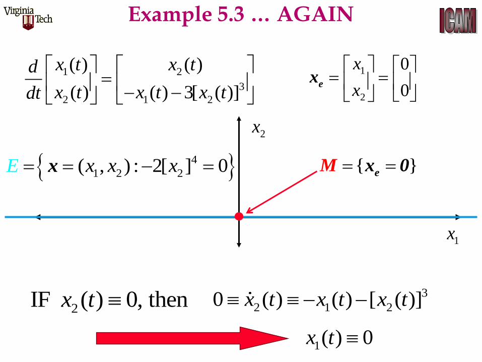
1 2
3
2 1 2
( ) ( )
( ) ( ) 3[ ( )]
x t x td
x t x t x tdt
1x
2x
4
1 2 2( , ) : 2[ ] 0x x xE x { } e
M x 0
2IF ( ) 0, thenx t 3
2 1 20 ( ) ( ) [ ( )]x t x t x t
1( ) 0x t
1
2
0
0
x
x
e
x
Example 5.3 … AGAIN
1x
2x
4
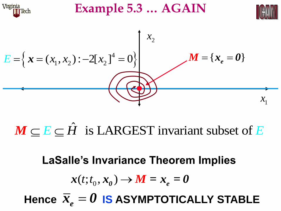
1 2 2( , ) : 2[ ] 0x x xE x { } e
M x 0
ˆ is LARGEST invariant subset of E EH M
0( ; , )t t 0 ex x M = x = 0
LaSalle’s Invariance Theorem Implies
Hence IS ASYMPTOTICALLY STABLE e
x 0
Example 5.3 … AGAIN
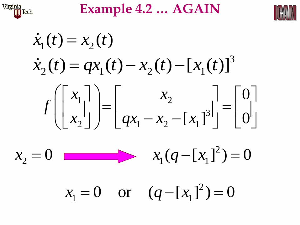
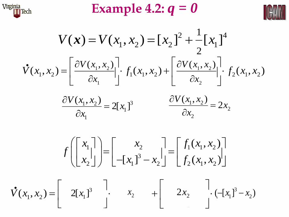
1 2( ) ( )x t x t3
2 1 2 1( ) ( ) ( ) [ ( )] x t qx t x t x t
1 2
3
2 1 2 1
0
[ ] 0
x xf
x qx x x
2 0x 2
1 1( [ ] ) 0 x q x
2
1 10 or ( [ ] ) 0 x q x
Example 4.2 … AGAIN
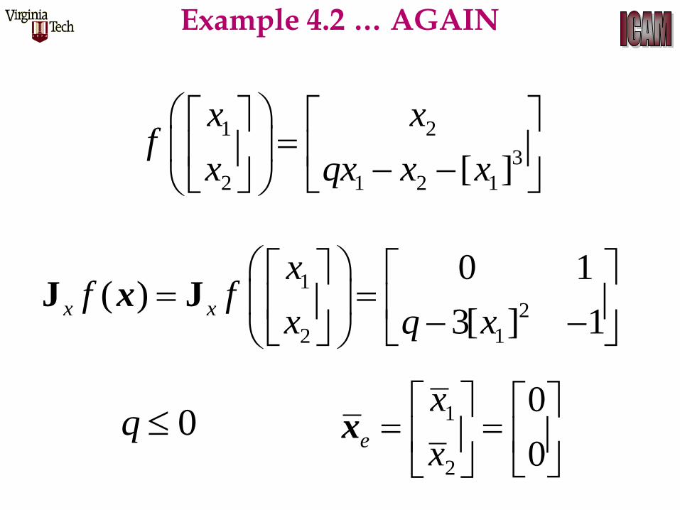
1 2
3
2 1 2 1[ ]
x xf
x qx x x
1
2
2 1
0 1( )
3[ ] 1
x x
xf f
x q xJ Jx
1
2
0
0e
x
x
x0q
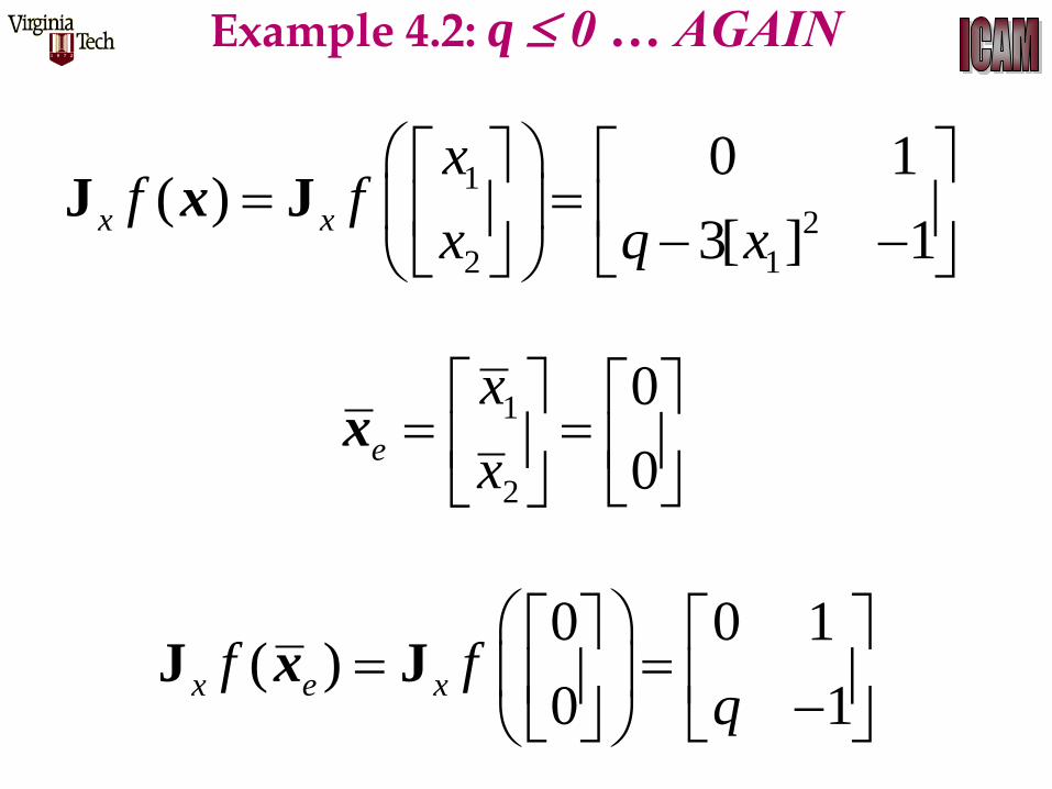
Example 4.2 … AGAIN
1
2
2 1
0 1( )
3[ ] 1
x x
xf f
x q xJ Jx
1
2
0
0e
x
x
x
0 0 1( )
0 1J Jx e xf f
q
x
Example 4.2: q 0 … AGAIN
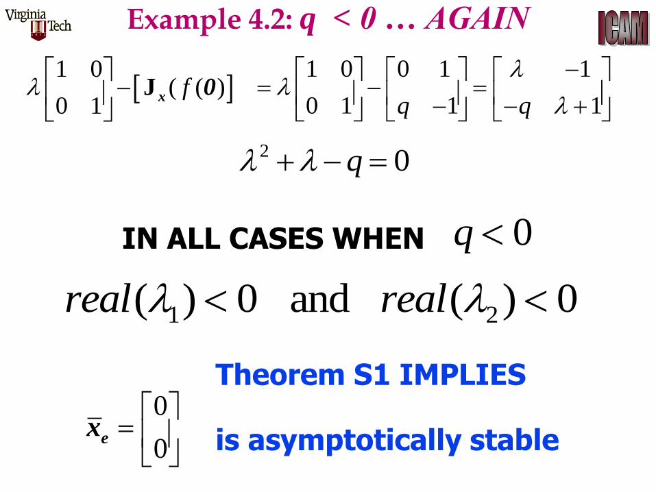
1 0 0 1 1
0 1 1 1q q
2 0 q
Example 4.2: q < 0 … AGAIN
1 0
( ( )0 1
J f
x 0
Theorem S1 IMPLIES 0
0
ex is asymptotically stable
1 2( ) 0 and ( ) 0real real
IN ALL CASES WHEN 0q
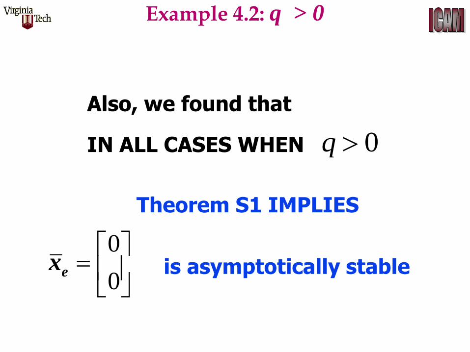
Theorem S1 IMPLIES
0
0
ex is asymptotically stable
IN ALL CASES WHEN 0q
Example 4.2: q > 0
Also, we found that
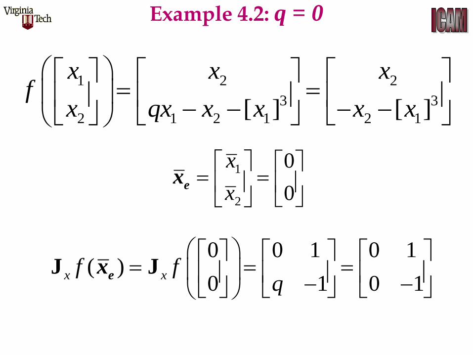
1 2 2
3 3
2 1 2 1 2 1[ ] [ ]
x x xf
x qx x x x x
1
2
0
0
x
x
ex
0 0 1 0 1( )
0 1 0 1J Jx xf f
q
ex
Example 4.2: q = 0
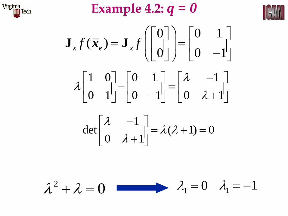
0 0 1( )
0 0 1J Jx xf f
ex
1 0 0 1 1
0 1 0 1 0 1
1det ( 1) 0
0 1
2 0 1 0 1 1
Example 4.2: q = 0
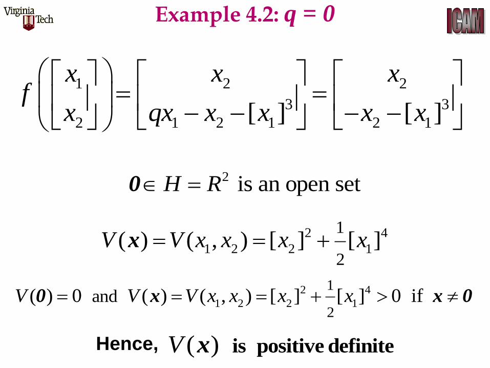
2 4
1 2 2 1
1
2( ) ( , ) [ ] [ ]V V x x x x x
2 is an open setH R 0
2 4
1 2 2 1
1
2and( ) 0 ( ) ( , ) [ ] [ ] 0 if V V V x x x x 0 x x 0
Hence, ( ) V is positive definitex
1 2 2
3 3
2 1 2 1 2 1[ ] [ ]
x x xf
x qx x x x x
Example 4.2: q = 0
1 2 1 1 2
3
2 1 2 2 1 2
( , )
[ ] ( , )
x x f x xf
x x x f x x
1 2 1 2
1 2
1 2 1 1 2 2 1 2
( , ) ( , )( , ) ( , ) ( , )
V x x V x x
x xV x x f x x f x x
.
31 21
1
( , )2[ ]
V x xx
x
1 22
2
( , )2
V x xx
x
1 2 1 2
1 2
1 2 1 1 2 2 1 2
( , ) ( , )( , ) ( , ) ( , )
V x x V x x
x xV x x f x x f x x
. 3
12[ ]x 22x2x 3
1 2( [ ] )x x
2 4
1 2 2 1
1
2( ) ( , ) [ ] [ ]V V x x x x x
Example 4.2: q = 0
1 2 1 2
1 2
1 2 1 1 2 2 1 2
( , ) ( , )( , ) ( , ) ( , )
V x x V x x
x xV x x f x x f x x
. 3
12[ ]x 22x2x 3
1 2( [ ] )x x
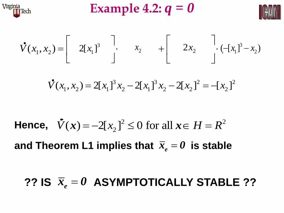
3 3 2 2
1 2 1 2 1 2 2 2( , ) 2[ ] 2[ ] 2[ ] [ ]V x x x x x x x x .
e
x 0
Hence, 2 2
2( ) 2[ ] 0 for all V x H R x x.
and Theorem L1 implies that is stable
?? IS ASYMPTOTICALLY STABLE ?? e
x 0
Example 4.2: q = 0
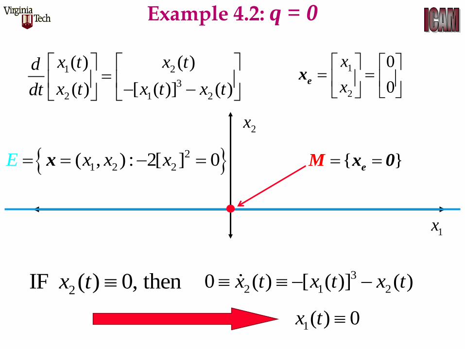
1 2
3
2 1 2
( ) ( )
( ) [ ( )] ( )
x t x td
x t x t x tdt
1x
2x
2
1 2 2( , ) : 2[ ] 0x x xE x { } e
M x 0
2IF ( ) 0, thenx t 3
2 1 20 ( ) [ ( )] ( )x t x t x t
1( ) 0x t
1
2
0
0
x
x
e
x
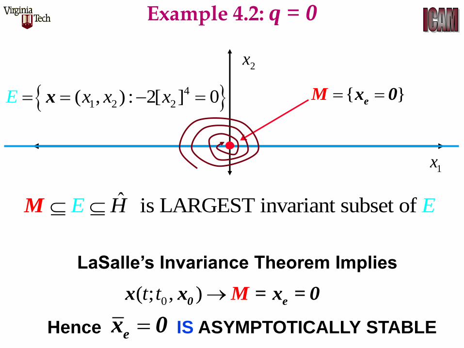
Example 4.2: q = 0
1x
2x
4
1 2 2( , ) : 2[ ] 0x x xE x { } e
M x 0
ˆ is LARGEST invariant subset of E EH M
0( ; , )t t 0 ex x M = x = 0
LaSalle’s Invariance Theorem Implies
Hence IS ASYMPTOTICALLY STABLE e
x 0
Example 4.2: q = 0
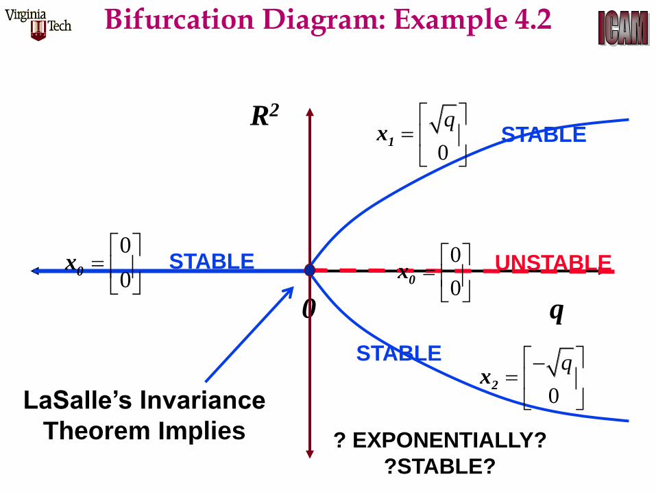
q 0
R2
0
0
0x
0
q
1x
0
q
2x
STABLE UNSTABLE
STABLE
STABLE
0
0
0x
LaSalle’s Invariance
Theorem Implies ? EXPONENTIALLY?
?STABLE?
Bifurcation Diagram: Example 4.2
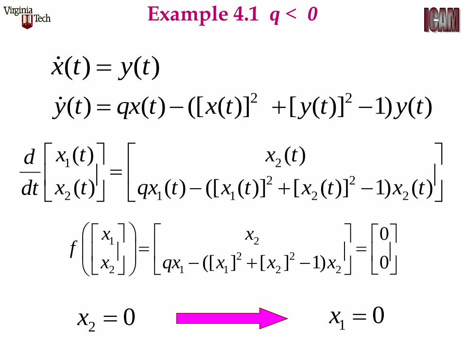
( ) ( )x t y t2 2( ) ( ) ([ ( )] [ ( )] 1) ( )y t qx t x t y t y t
1 2
2 2
2 1 1 2 2
( ) ( )
( ) ( ) ([ ( )] [ ( )] 1) ( )
x t x td
x t qx t x t x t x tdt
1 2
2 2
2 1 1 2 2
0
([ ] [ ] 1) 0
x xf
x qx x x x
2 0x 1 0x
Example 4.1 q < 0
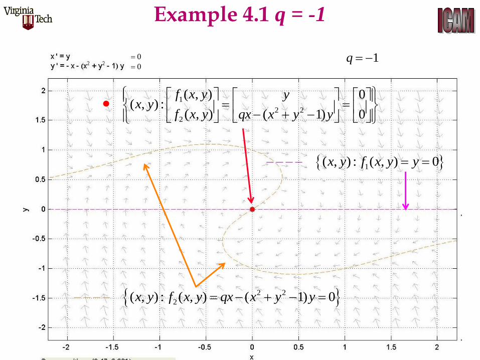
Example 4.1 q = -1
0
0
1 ( , ) : ( , ) 0x y f x y y
2 2
2 ( , ) : ( , ) ( 1) 0x y f x y qx x y y
1
2 2
2
( , ) 0 ( , ) :
( , ) ( 1) 0
f x y yx y
f x y qx x y y
1q
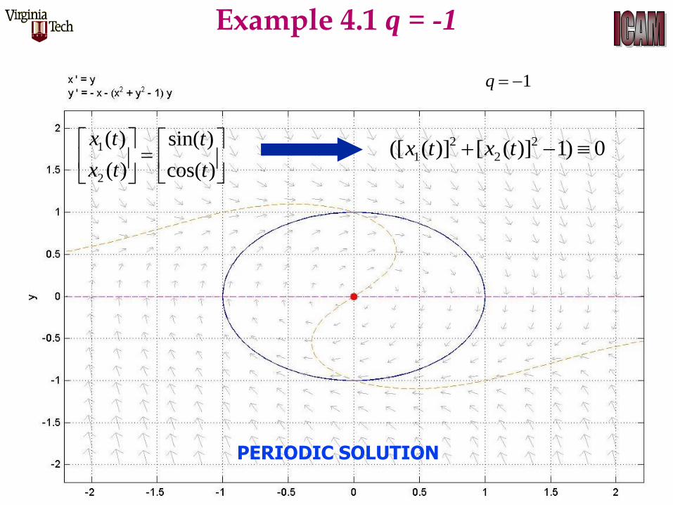
Example 4.1 q = -1
1
2
( ) sin( )
( ) cos( )
x t t
x t t
PERIODIC SOLUTION
1q
2 2
1 2([ ( )] [ ( )] 1) 0x t x t
Example 4.1 q = -1
1
2
( ) sin( )
( ) cos( )
x t t
x t t
1q
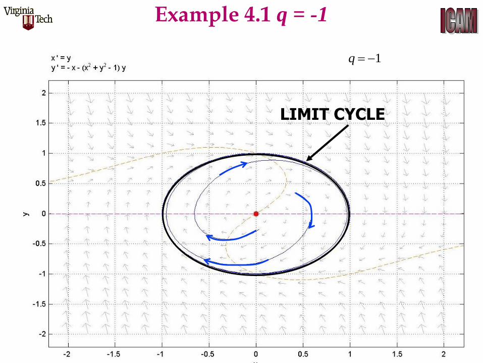
LIMIT CYCLE
Example 4.1 q = -1
1q
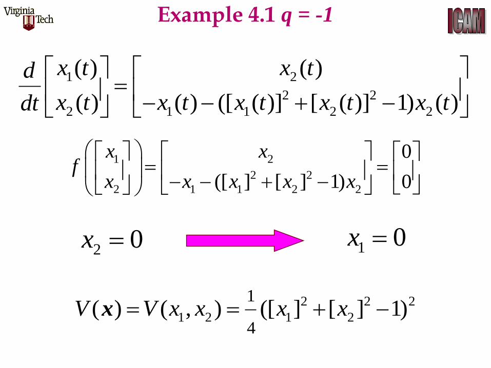
Example 4.1 q = -1
1 2
2 2
2 1 1 2 2
( ) ( )
( ) ( ) ([ ( )] [ ( )] 1) ( )
x t x td
x t x t x t x t x tdt
1 2
2 2
2 1 1 2 2
0
([ ] [ ] 1) 0
x xf
x x x x x
2 0x 1 0x
2 2 2
1 2 1 2
1
4( ) ( , ) ([ ] [ ] 1)V V x x x x x

Example 4.1 q = -1
2 21 21 1 2
1
( , )([ ] [ ] 1)
V x xx x x
x
2 21 22 1 2
2
( , )([ ] [ ] 1)
V x xx x x
x
1 2 1 2
1 2
1 2 1 1 2 2 1 2
( , ) ( , )( , ) ( , ) ( , )
V x x V x x
x xV x x f x x f x x
.
1 2
2 2
2 1 1 2 2
0
([ ] [ ] 1) 0
x xf
x x x x x
2 2 2
1 2 1 2
1
4( ) ( , ) ([ ] [ ] 1)V V x x x x x
2 2 2 2 2 2 2 2
1 2 1 2 1 2 1 2 1 2 1 2 2( , ) ([ ] [ ] 1) ([ ] [ ] 1) ([ ] [ ] 1)V x x x x x x x x x x x x x .
2 2
1 1 2 2( ([ ] [ ] 1) )x x x x 2x2 2
1 1 2([ ] [ ] 1)x x x 2 2
2 1 2([ ] [ ] 1)x x x
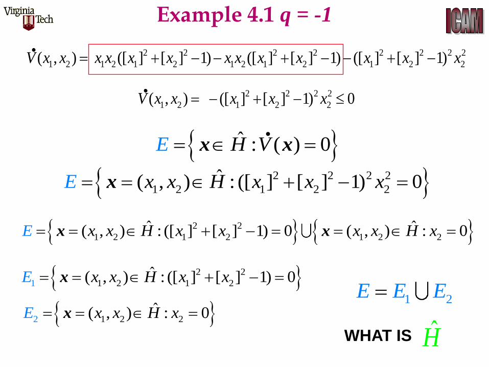
Example 4.1 q = -1
2 2 2 2 2 2 2 2
1 2 1 2 1 2 1 2 1 2 1 2 2( , ) ([ ] [ ] 1) ([ ] [ ] 1) ([ ] [ ] 1)V x x x x x x x x x x x x x .
2 2 2 2
1 2 1 2 2( , ) ([ ] [ ] 1) 0V x x x x x .
2 2 2 2
1 2 1 2 2ˆ( , ) : ([ ] [ ] 1) 0x x x xE H x x
ˆ : ( ) 0H VE x x.
2 2
1 2 1 2 1 2 2ˆ ˆ( , ) : ([ ] [ ] 1) 0 ( , ) : 0x x H x x x x xE H x x
2 2
1 2 11 2ˆ( , ) : ([ ] [ ] 1) 0x x H x xE x
1 2E E E 1 22 2
ˆ( , ) : 0x x H xE x
WHAT IS H
Example 4.1 q = -1
1 2( , ) : ( )ˆ 2x x VH x
2 2 2
1 2 1 2
1
4( ) ( , ) ([ ] [ ] 1)V V x x x x x
1E
2E
2 { } e
x 0M
11
2 2
2 1 2{ [ , ] ([ ] [ ] 1) }Tx x x x x =M : 0
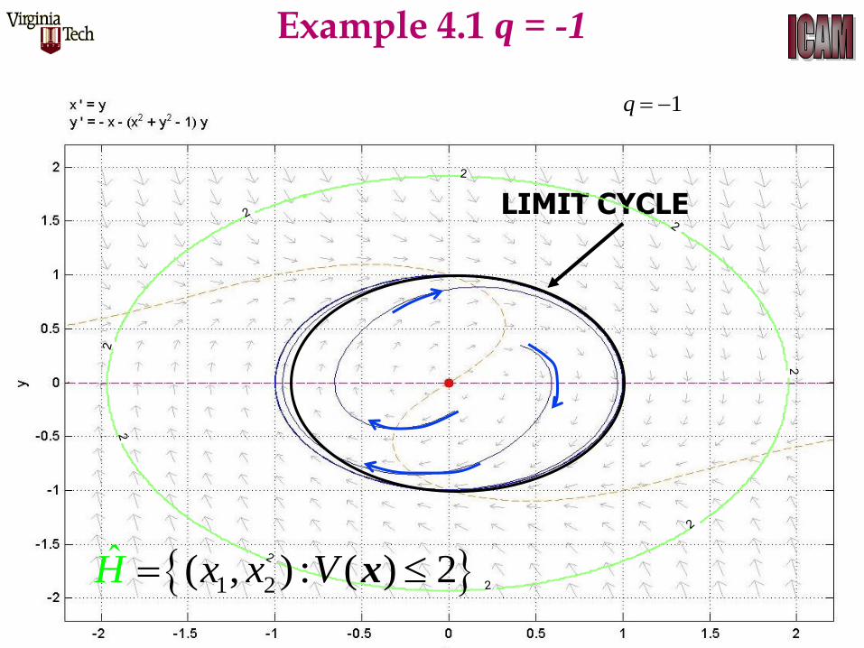
LIMIT CYCLE
Example 4.1 q = -1
1q
1 2( , ) : ( )ˆ 2x x VH x
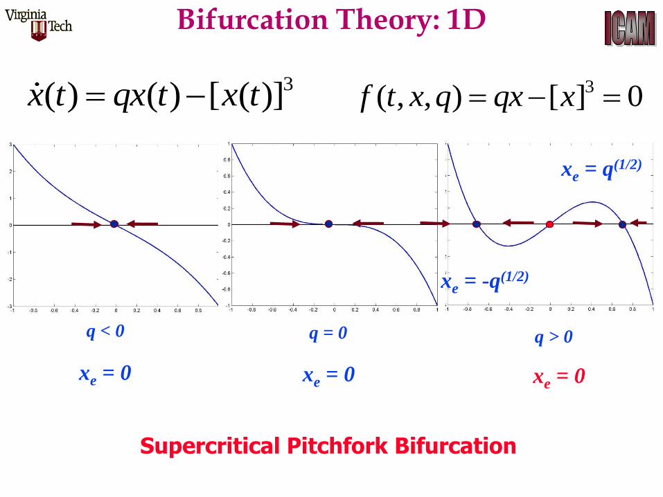
3( ) ( ) [ ( )]x t qx t x t 3( , , ) [ ] 0f t x q qx x
q < 0 q > 0 q = 0
xe = 0 xe = 0
xe = -q(1/2)
xe = 0
xe = q(1/2)
Supercritical Pitchfork Bifurcation
Bifurcation Theory: 1D
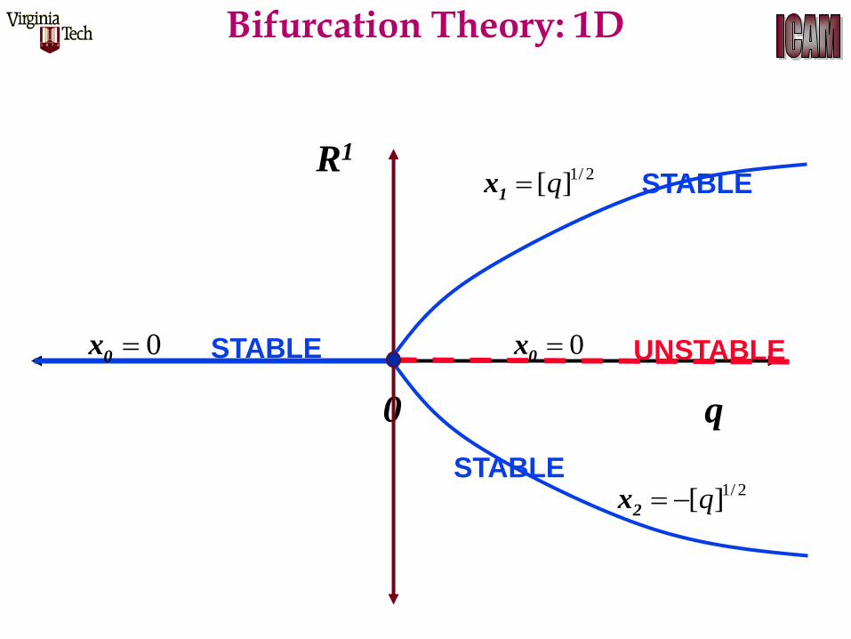
q 0
R1
00x
1/ 2[ ]q1x
1/ 2[ ]q 2x
STABLE UNSTABLE
STABLE
STABLE
00x
Bifurcation Theory: 1D
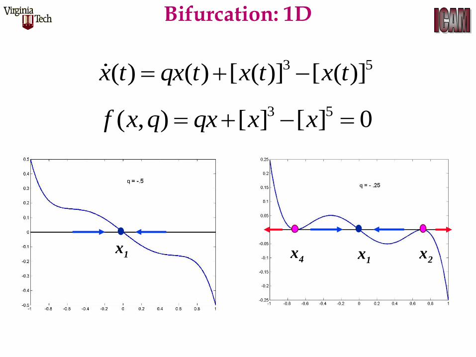
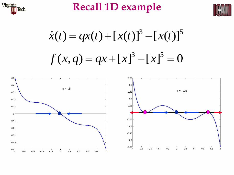
3 5( ) ( ) [ ( )] [ ( )]x t qx t x t x t
3 5( , ) [ ] [ ] 0f x q qx x x
Bifurcation: 1D
1x
1x4
x2
x
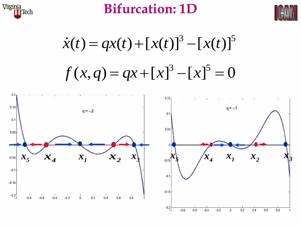
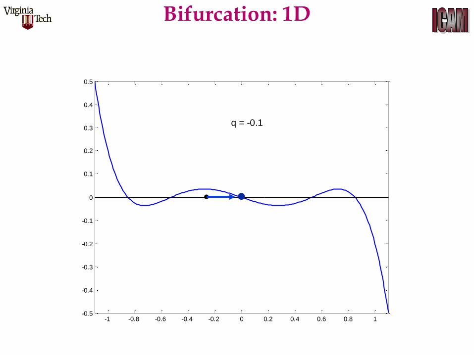
3 5( ) ( ) [ ( )] [ ( )]x t qx t x t x t
3 5( , ) [ ] [ ] 0f x q qx x x
Bifurcation: 1D
1x
4x 2
x 3x
5x
1x
4x 2
x 3x
5x
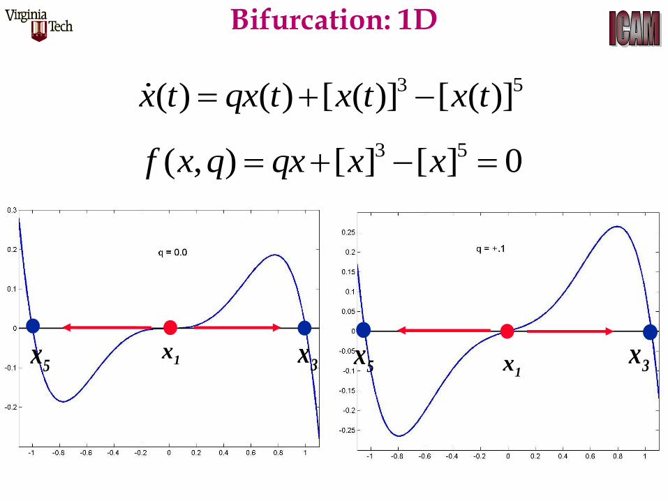
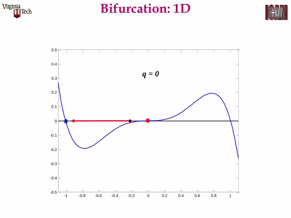
3 5( ) ( ) [ ( )] [ ( )]x t qx t x t x t
3 5( , ) [ ] [ ] 0f x q qx x x
Bifurcation: 1D
3x
5x 3
x5
x1x
1x
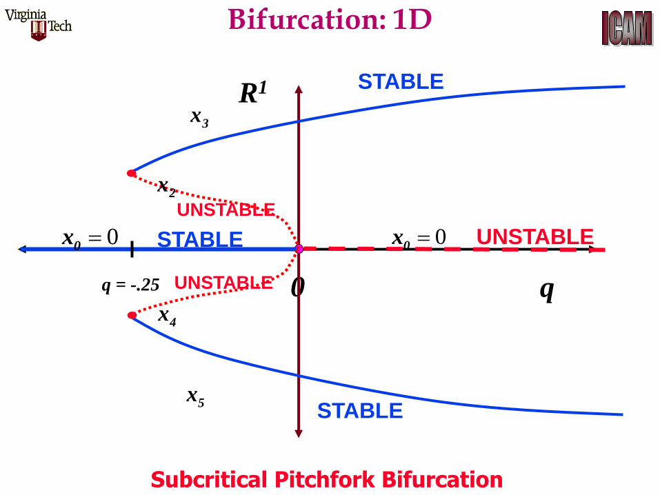
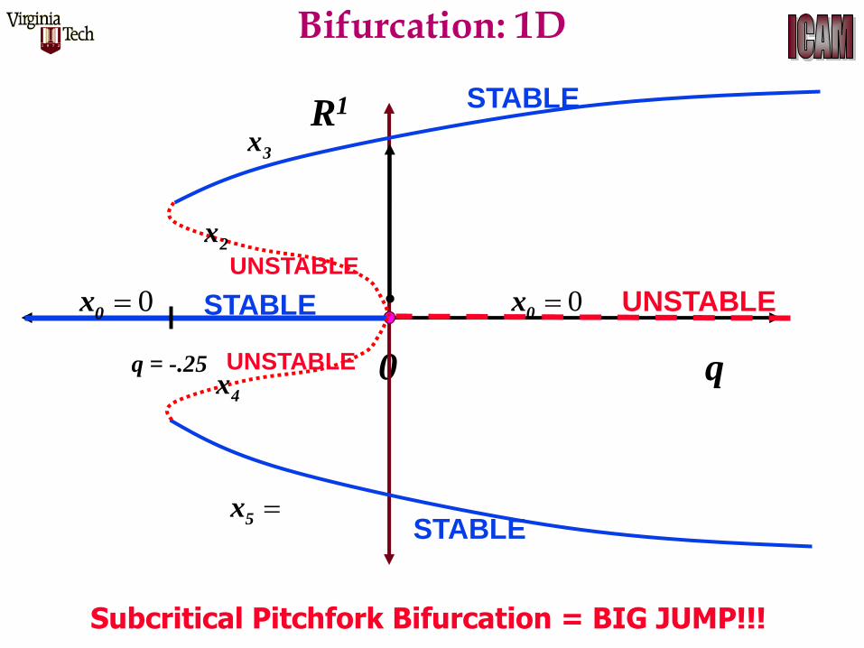
q 0
R1
00x
3x
5x
STABLE UNSTABLE
STABLE
STABLE
00x
q = -.25
2x
4x
UNSTABLE
UNSTABLE
Subcritical Pitchfork Bifurcation
Bifurcation: 1D
-1 -0.8 -0.6 -0.4 -0.2 0 0.2 0.4 0.6 0.8 1-0.5
-0.4
-0.3
-0.2
-0.1
0
0.1
0.2
0.3
0.4
0.5
q = -0.1
Bifurcation: 1D
-1 -0.8 -0.6 -0.4 -0.2 0 0.2 0.4 0.6 0.8 1-0.5
-0.4
-0.3
-0.2
-0.1
0
0.1
0.2
0.3
0.4
0.5
q = 0
Bifurcation: 1D
q 0
R1
00x
3x
5x
STABLE UNSTABLE
STABLE
STABLE
00x
q = -.25
2x
4xUNSTABLE
UNSTABLE
Subcritical Pitchfork Bifurcation = BIG JUMP!!!
Bifurcation: 1D
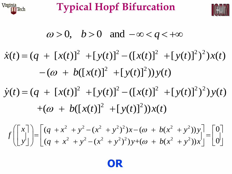
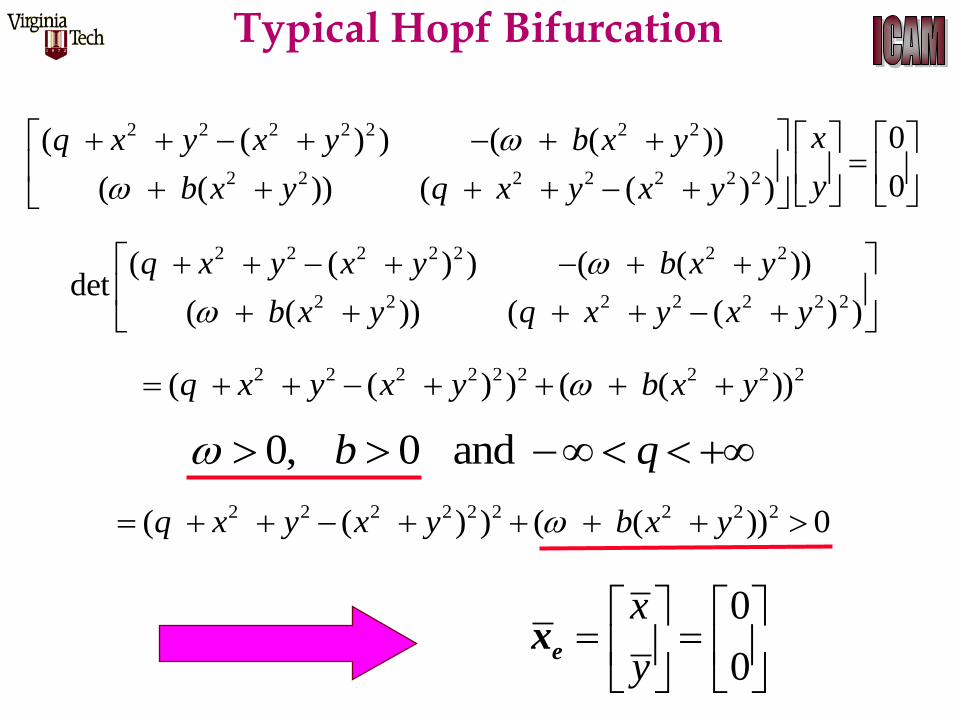
2 2 2 2 2
2 2
( ) ( [ ( )] [ ( )] ([ ( )] [ ( )] ) ) ( )
( ([ ( )] [ ( )] )) ( )
x t q x t y t x t y t x t
b x t y t y t
2 2 2 2 2 2 2
2 2 2 2 2 2 2
0( ( ) ) ( ( ))
0( ( ) ) +( ( ))
x q x y x y x b x y yf
y q x y x y y b x y x
2 2 2 2 2
2 2
( ) ( [ ( )] [ ( )] ([ ( )] [ ( )] ) ) ( )
+( ([ ( )] [ ( )] )) ( )
y t q x t y t x t y t y t
b x t y t x t
0, 0 and b q
OR
Typical Hopf Bifurcation
2 2 2 2 2 2 2
2 2 2 2 2 2 2
0( ( ) ) ( ( ))
0( ( )) ( ( ) )
xq x y x y b x y
yb x y q x y x y
2 2 2 2 2 2 2
2 2 2 2 2 2 2
( ( ) ) ( ( ))det
( ( )) ( ( ) )
q x y x y b x y
b x y q x y x y
2 2 2 2 2 2 2 2 2( ( ) ) ( ( ))q x y x y b x y
0
0
x
y
ex
0, 0 and b q
2 2 2 2 2 2 2 2 2( ( ) ) ( ( )) 0q x y x y b x y
Typical Hopf Bifurcation
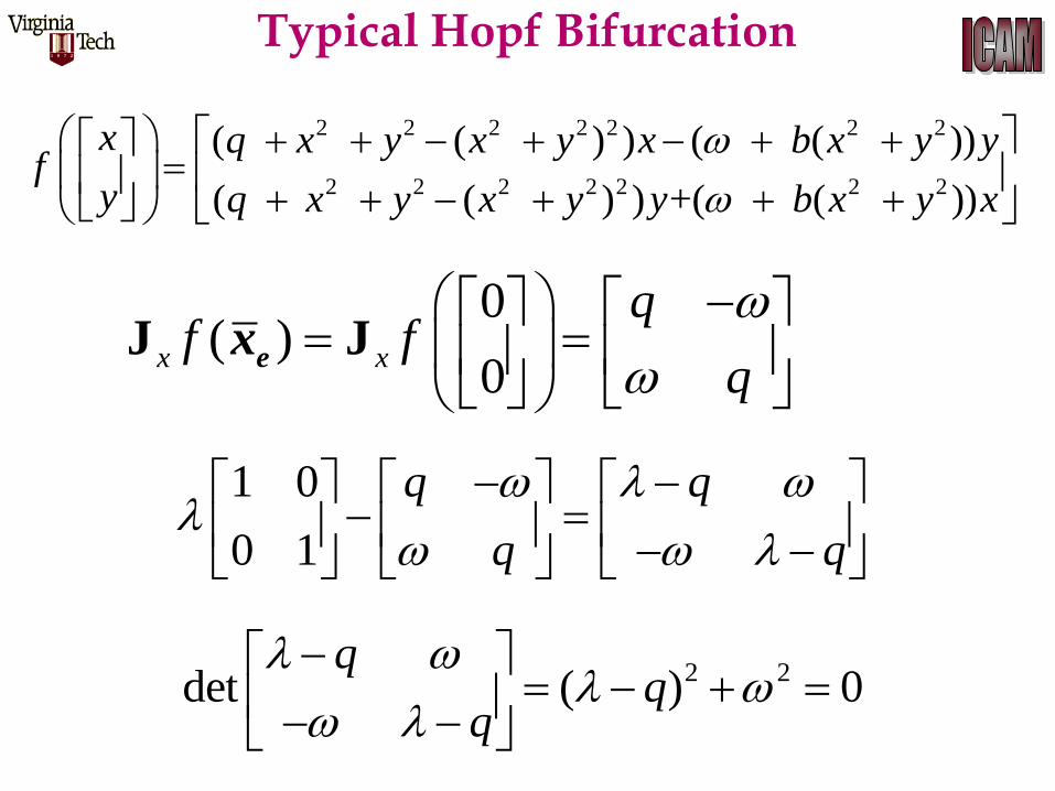
0( )
0J Jx x
qf f
q
ex
2 2 2 2 2 2 2
2 2 2 2 2 2 2
( ( ) ) ( ( ))
( ( ) ) +( ( ))
x q x y x y x b x y yf
y q x y x y y b x y x
1 0
0 1
q q
q q
2 2det ( ) 0q
Typical Hopf Bifurcation
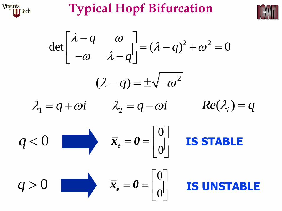
2 2det ( ) 0q
2( )q
1 q i 2 q i
0q 0
0
ex 0 IS STABLE
0q 0
0
ex 0 IS UNSTABLE
( )iRe q
Typical Hopf Bifurcation
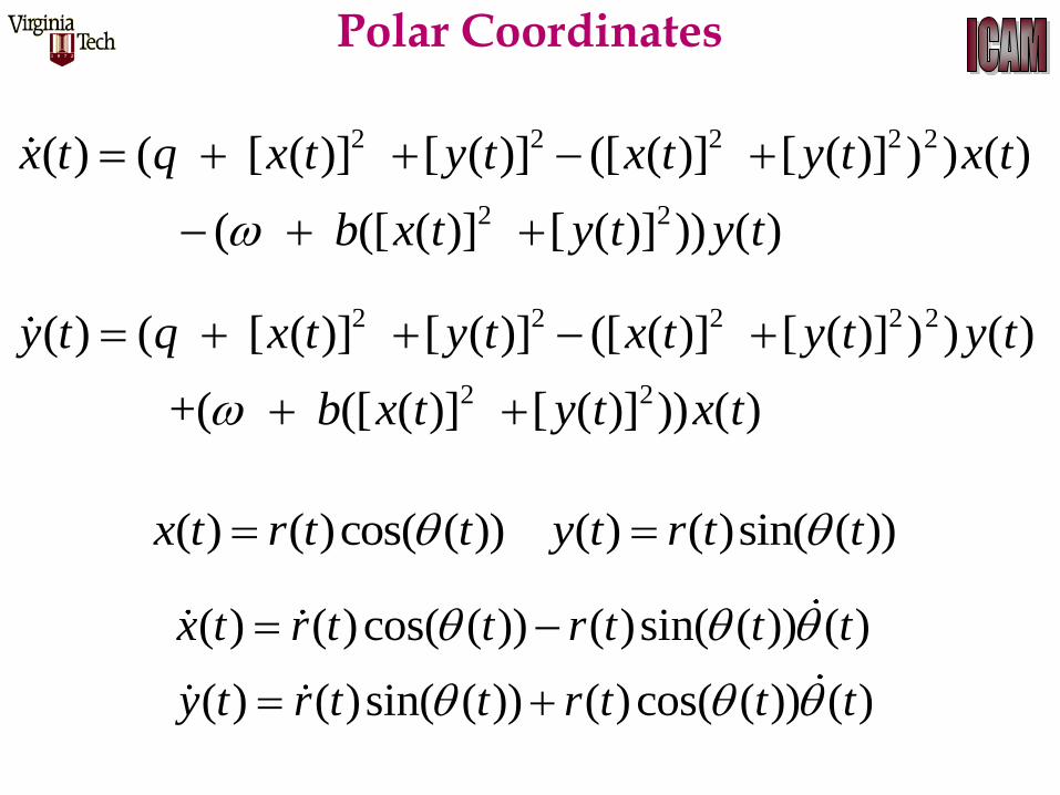
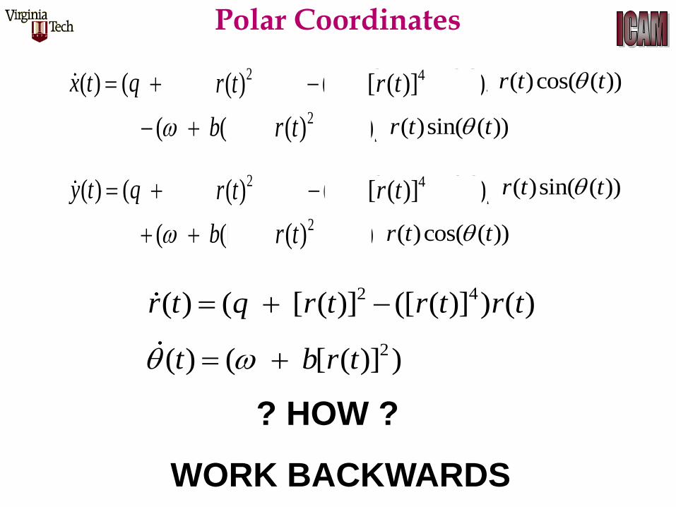
2 2 2 2 2
2 2
( ) ( [ ( )] [ ( )] ([ ( )] [ ( )] ) ) ( )
( ([ ( )] [ ( )] )) ( )
x t q x t y t x t y t x t
b x t y t y t
2 2 2 2 2
2 2
( ) ( [ ( )] [ ( )] ([ ( )] [ ( )] ) ) ( )
+( ([ ( )] [ ( )] )) ( )
y t q x t y t x t y t y t
b x t y t x t
( ) ( )cos( ( )) ( )sin( ( )) ( )
( ) ( )sin( ( )) ( )cos( ( )) ( )
x t r t t r t t t
y t r t t r t t t
( ) ( )cos( ( )) ( ) ( )sin( ( ))x t r t t y t r t t
Polar Coordinates
2 2 2 2 2
2 2
( ) ( [ ( )] [ ( )] ([ ( )] [ ( )] ) ) ( )
( ([ ( )] [ ( )] )) ( )
x t q x t y t x t y t x t
b x t y t y t
2( )r t 4[ ( )]r t ( )cos( ( ))r t t
2( )r t ( )sin( ( ))r t t
2 4( ) ( [ ( )] ([ ( )] ) ( )r t q r t r t r t
2( ) ( [ ( )] )t b r t
2 2 2 2 2
2 2
( ) ( [ ( )] [ ( )] ([ ( )] [ ( )] ) ) ( )
( ([ ( )] [ ( )] )) ( )
y t q x t y t x t y t y t
b x t y t x t
2( )r t 4[ ( )]r t
( )cos( ( ))r t t2( )r t
( )sin( ( ))r t t
Polar Coordinates
? HOW ?
WORK BACKWARDS
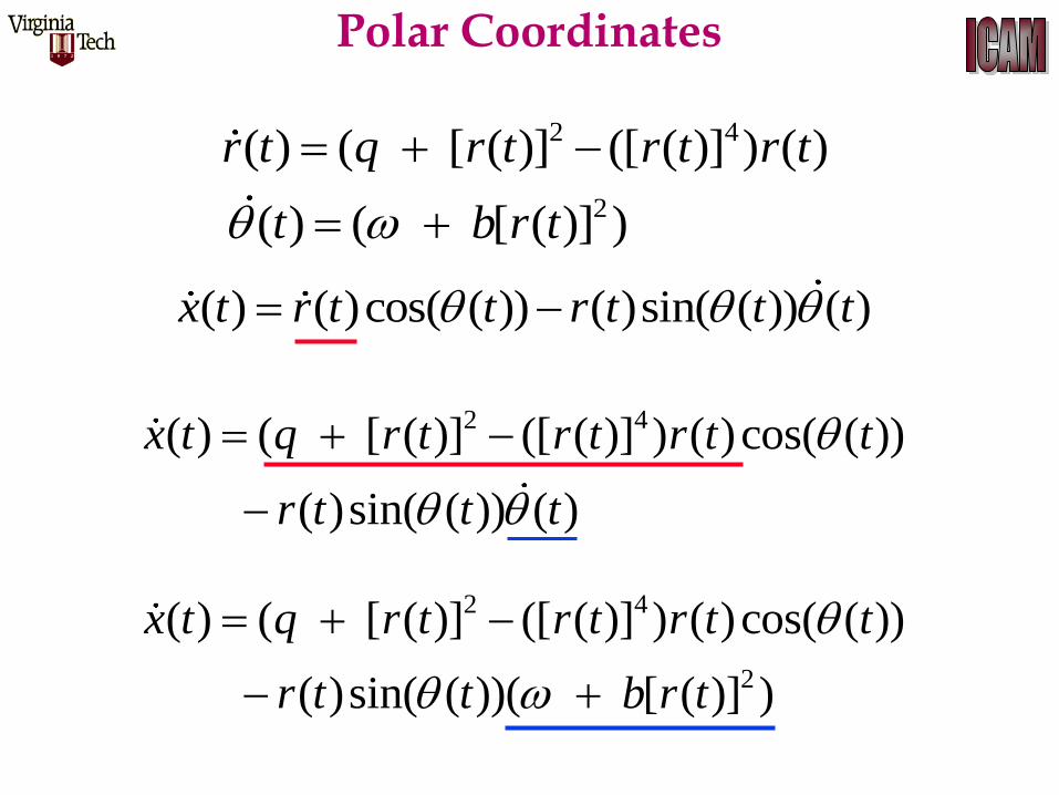
2 4( ) ( [ ( )] ([ ( )] ) ( )r t q r t r t r t
2( ) ( [ ( )] )t b r t
2 4( ) ( [ ( )] ([ ( )] ) ( )cos( ( ))
( )sin( ( )) ( )
x t q r t r t r t t
r t t t
( ) ( )cos( ( )) ( )sin( ( )) ( )x t r t t r t t t
2 4
2
( ) ( [ ( )] ([ ( )] ) ( )cos( ( ))
( )sin( ( ))( [ ( )] )
x t q r t r t r t t
r t t b r t
Polar Coordinates

2 2 2( ) cos( ) sin( )r x y x r y r
2 4
2
( ) ( [ ( )] ([ ( )] ) ( )cos( ( ))
( )sin( ( ))( [ ( )] )
x t q r t r t r t t
r t t b r t
2 2 2 2 2
2 2
( ) ( ([ ( )] [ ( )] ) (([ ( )] [ ( )] ) ) ( )cos( ( ))
( )sin( ( ))( ([ ( )] [ ( )] ))
x t q x t y t x t y t r t t
r t t b x t y t
2 2 2 2 2
2 2
( ) ( ([ ( )] [ ( )] ) (([ ( )] [ ( )] ) ) ( )
( )( ([ ( )] [ ( )] ))
x t q x t y t x t y t x t
y t b x t y t
Polar Coordinates
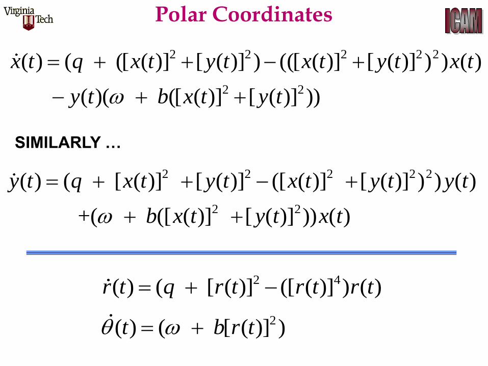
2 2 2 2 2
2 2
( ) ( ([ ( )] [ ( )] ) (([ ( )] [ ( )] ) ) ( )
( )( ([ ( )] [ ( )] ))
x t q x t y t x t y t x t
y t b x t y t
2 2 2 2 2
2 2
( ) ( [ ( )] [ ( )] ([ ( )] [ ( )] ) ) ( )
+( ([ ( )] [ ( )] )) ( )
y t q x t y t x t y t y t
b x t y t x t
2 4( ) ( [ ( )] ([ ( )] ) ( )r t q r t r t r t
2( ) ( [ ( )] )t b r t
Polar Coordinates
SIMILARLY …
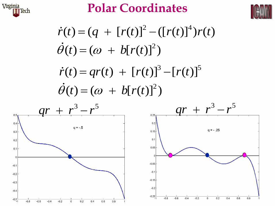
2 4( ) ( [ ( )] ([ ( )] ) ( )r t q r t r t r t 2( ) ( [ ( )] )t b r t
3 5( ) ( ) [ ( )] [ ( )]r t qr t r t r t 2( ) ( [ ( )] )t b r t
3 5 qr r r 3 5 qr r r
Polar Coordinates
3 5( ) ( ) [ ( )] [ ( )]x t qx t x t x t
3 5( , ) [ ] [ ] 0f x q qx x x
Recall 1D example
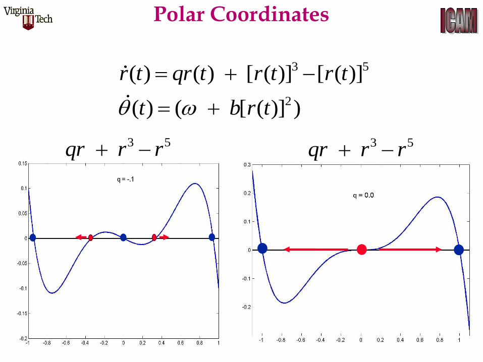
3 5( ) ( ) [ ( )] [ ( )]r t qr t r t r t
2( ) ( [ ( )] )t b r t
3 5 qr r r 3 5 qr r r
Polar Coordinates
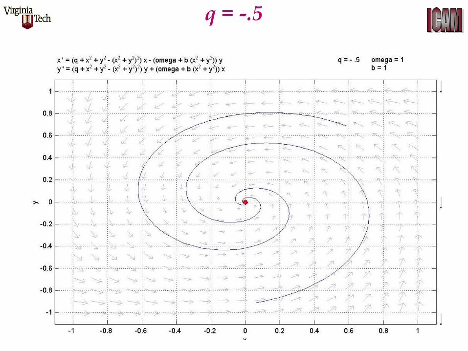
q = -.5
q = -.25
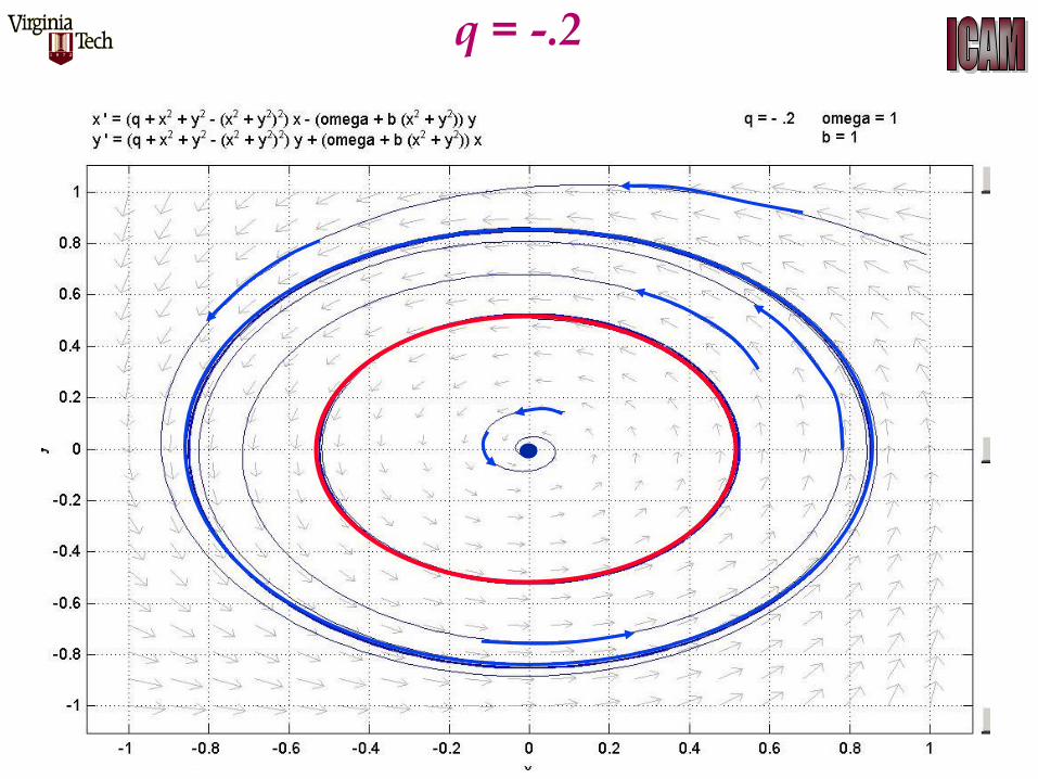
q = -.2
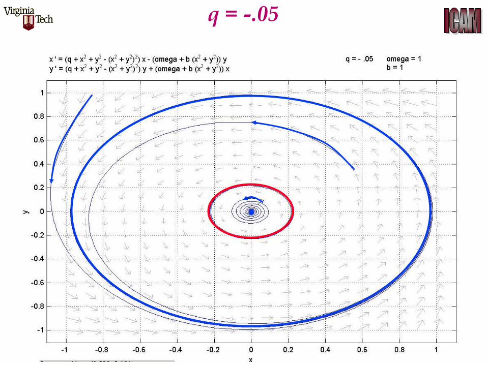
q = -.05
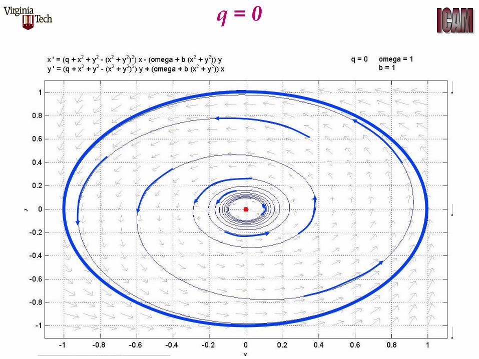
q = 0
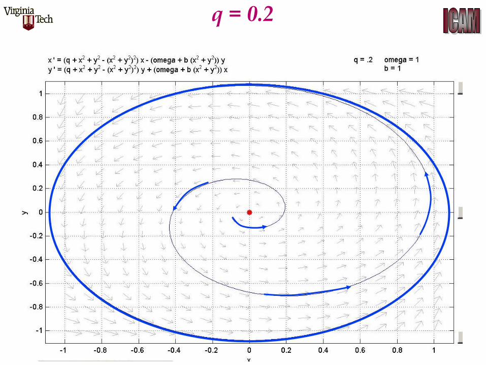
q = 0.2
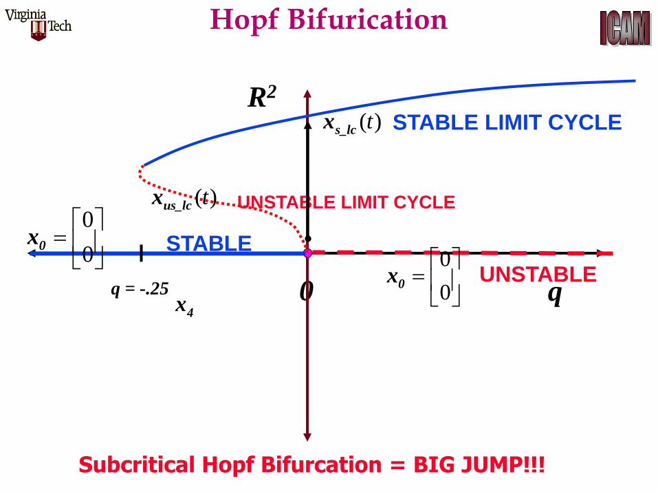
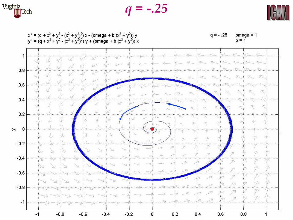
q 0
R2
0
0
0x
( )ts_lcx
STABLE
UNSTABLE
STABLE LIMIT CYCLE
0
0
0x
q = -.25
( )tus_lcx
4x
UNSTABLE LIMIT CYCLE
Subcritical Hopf Bifurcation = BIG JUMP!!!
Hopf Bifurication
Introduction to Dynamical Systems
Basic Ideas
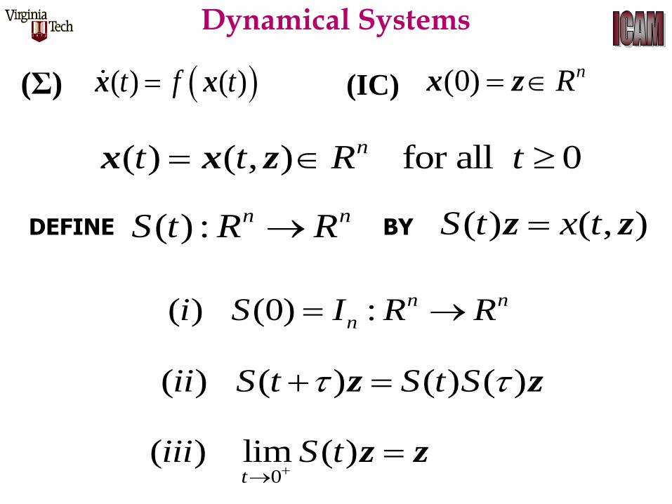
Dynamical Systems
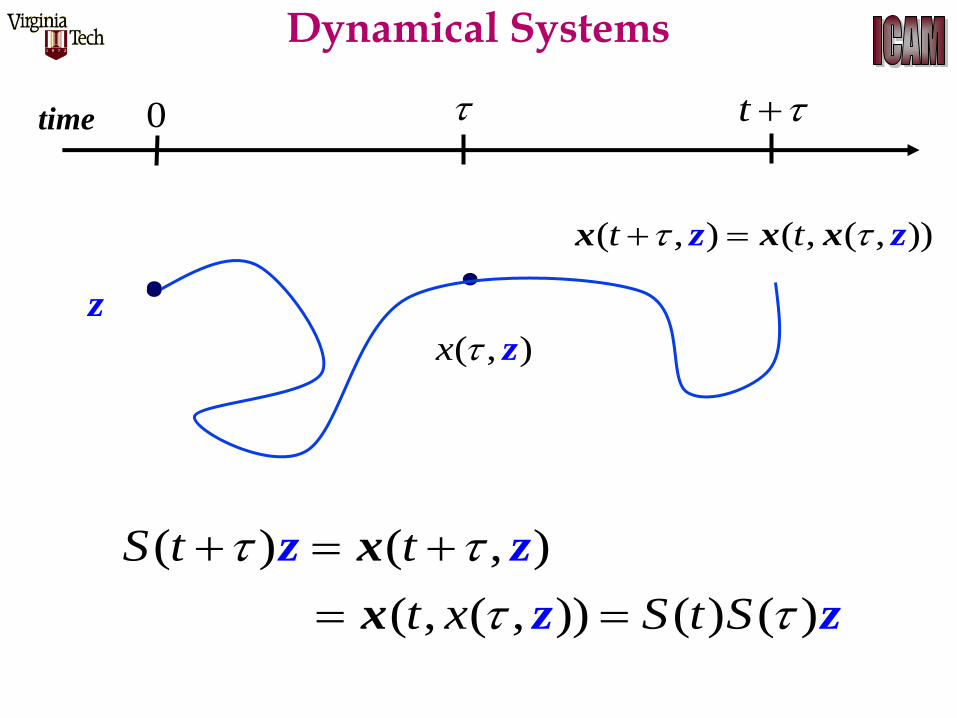
( ) ( , ) for all 0nt t R t x x z
(0) nR x z(IC) ( ) ( )t f tx x(Σ)
( ) ( , )S t x tz z( ) : n nS t R RDEFINE BY
( ) ( ) ( ) ( )ii S t S t S z z
( ) (0) : n n
ni S I R R
0( ) lim ( )
tiii S t
z z
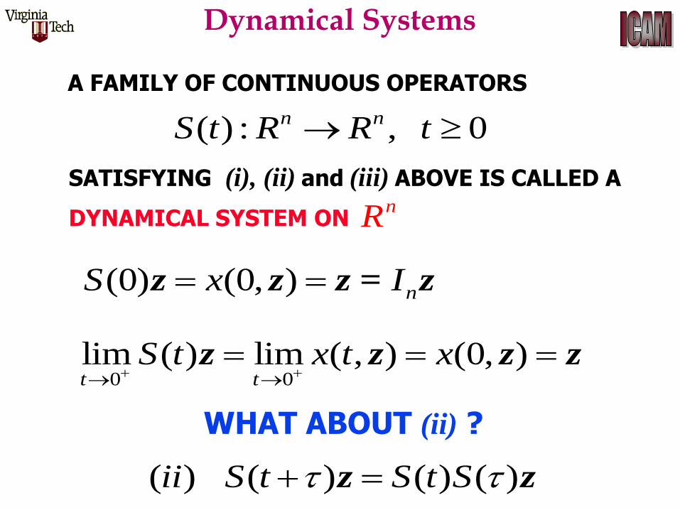
Dynamical Systems
0 0lim ( ) lim ( , ) (0, )t t
S t x t x
z z z z
(0) (0, ) nS x I z z z = z
WHAT ABOUT (ii) ?
( ) ( ) ( ) ( )ii S t S t S z z
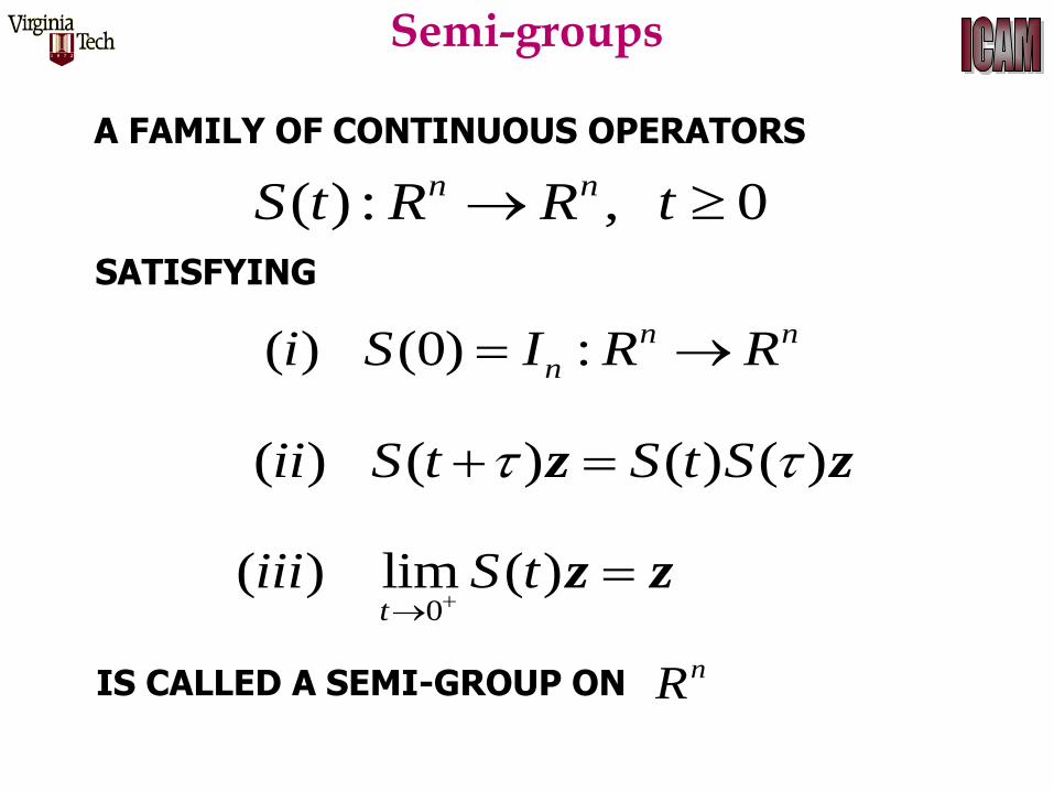
( ) : , 0n nS t R R t
A FAMILY OF CONTINUOUS OPERATORS
SATISFYING (i), (ii) and (iii) ABOVE IS CALLED A
DYNAMICAL SYSTEM ON nR
Dynamical Systems
( ) ( , )
( , ( , )) ( ) ( )
S t t
t x S t S
x
z
z
xz
z
z
( , ( , ))t x x z
( , )x z
0 time t
( , )t x z
Semi-groups
( ) ( ) ( ) ( )ii S t S t S z z
( ) (0) : n n
ni S I R R
0( ) lim ( )
tiii S t
z z
( ) : , 0 n nS t R R t
A FAMILY OF CONTINUOUS OPERATORS
SATISFYING
IS CALLED A SEMI-GROUP ON nR
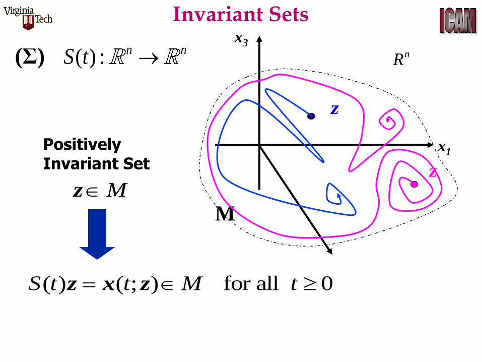
nR
x3
x1
M
z
z
( ) ( ; ) for all 0S t t M t z x z
Mz
( ) : n nS t (Σ)
Invariant Sets
Positively Invariant Set
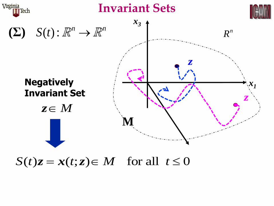
Invariant Sets
nR
x3
x1
M
z
z
( ) ( ; ) for all 0S t t M t z x z
Mz
Negatively Invariant Set
( ) : n nS t (Σ)
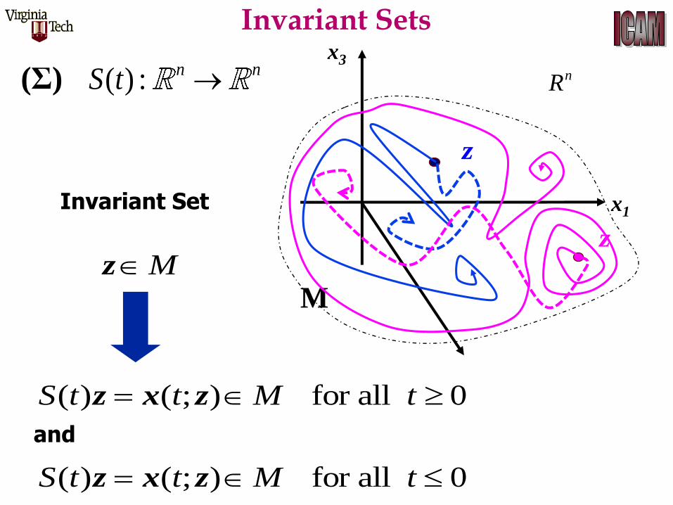
Invariant Sets
nR
x3
x1
M
z
z
( ) ( ; ) for all 0S t t M t z x z
Mz
Invariant Set
and
( ) ( ; ) for all 0S t t M t z x z
( ) : n nS t (Σ)
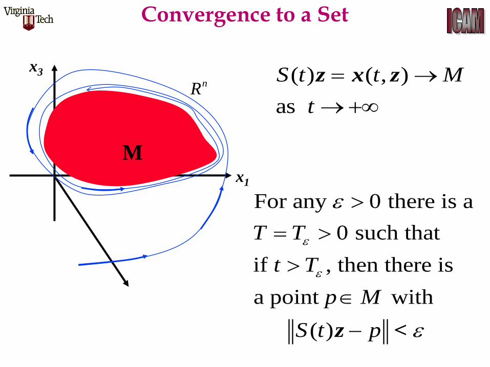
nR
x3
x1
( ) ( , )
as
S t t M
t
z x z
M
For any 0 there is a
0 such that
if , then there is
a point with
( )
T T
t T
p M
S t pz <
Convergence to a Set
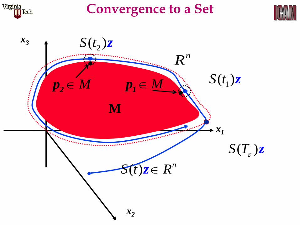
nR
x3
x1
x2
M
( ) nS t Rz
1( )S t zM1p
( )S T z
2( )S t z
M2p
Convergence to a Set
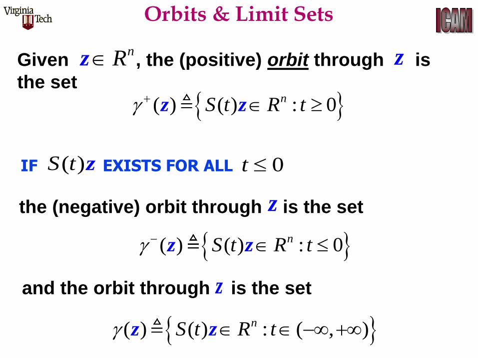
Given , the (positive) orbit through is
the set
nRz z
( ) ( ) : 0 nS t R tz z
the (negative) orbit through is the set
z
( ) ( ) : 0 nS t R tz z
and the orbit through is the set z
( ) ( ) : ( , ) nS t R tz z
Orbits & Limit Sets
IF EXISTS FOR ALL ( )S t z 0t
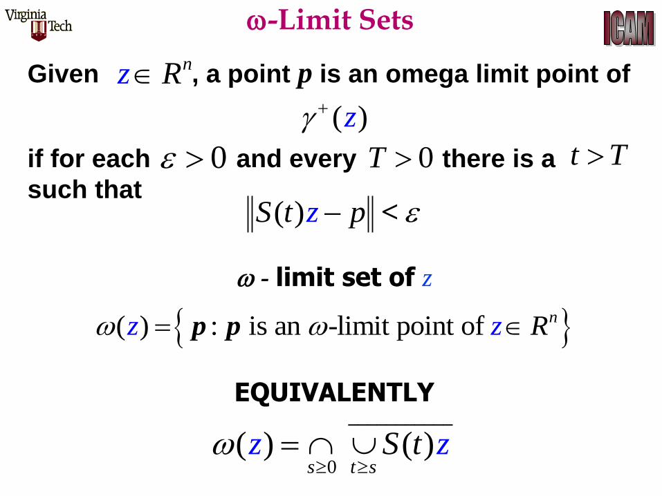
Given , a point p is an omega limit point of
if for each and every there is a
such that
nz R
( )z
0 0T t T
( )zS t p <
-Limit Sets
0( ) ( )
s t sz zS t
___________
EQUIVALENTLY
( ) : is an -limit point of nz z R p p
- limit set of z
-Limit Sets
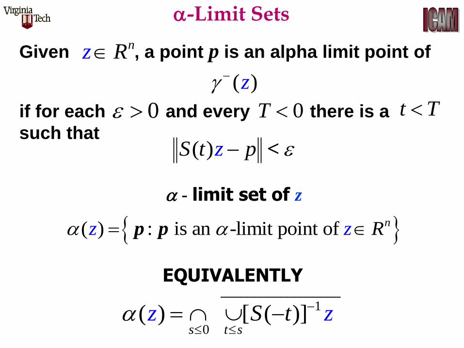
Given , a point p is an alpha limit point of
if for each and every there is a
such that
nz R
( )z
0 0T t T
( )zS t p <
1
0( ) [ ( )]
s t sz t zS
__________________EQUIVALENTLY
( ) : is an -limit point of nz z R p p
- limit set of z
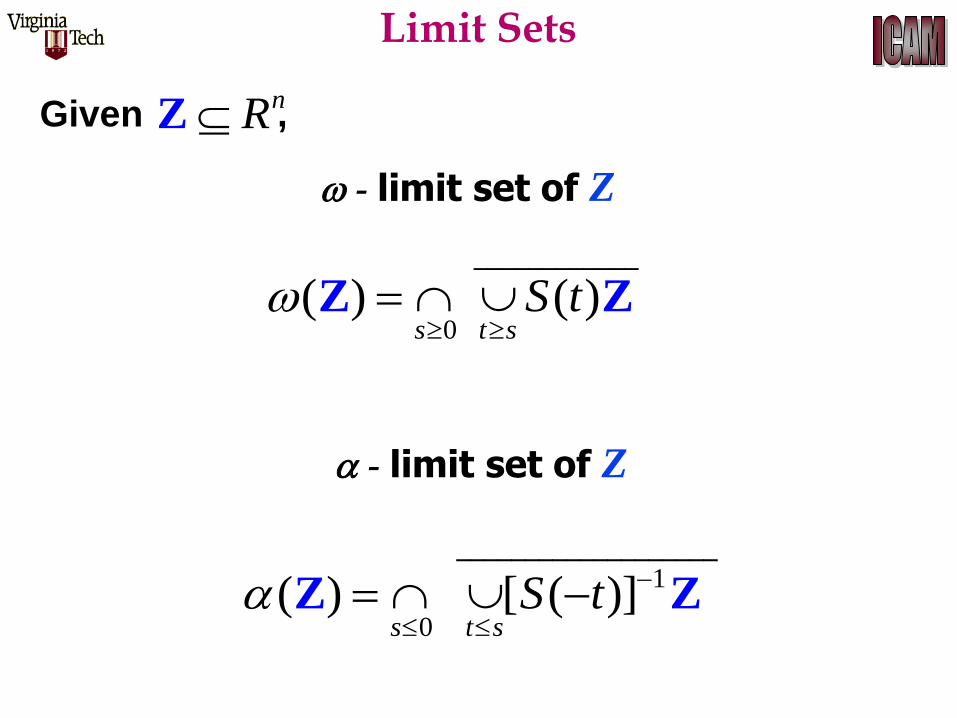
Given , nRZ
Limit Sets
0( ) ( )
s t sS t
Z Z
____________
- limit set of Z
- limit set of Z
1
0( ) [ ( )]
s t sS t
Z Z
___________________
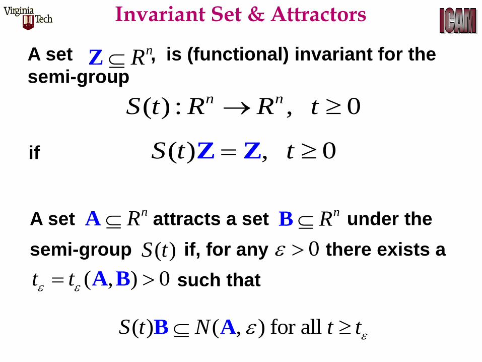
Invariant Set & Attractors
nRZ
( ) : , 0 n nS t R R t
if ( ) , 0S t t Z Z
A set , is (functional) invariant for the
semi-group
A set attracts a set under the
semi-group if, for any there exists a
such that
nRA
( ) ( , ) for all S t N t t B A
nRB
( )S t 0
( , ) 0t t A B
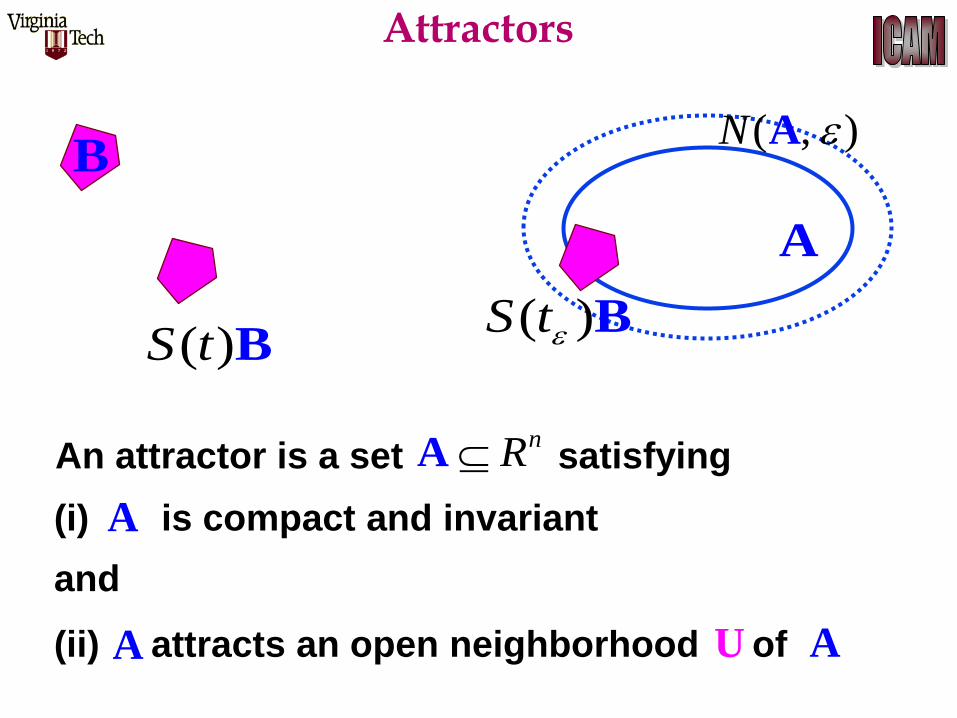
Attractors
( )S t B
B
( )S t B
A
( , )N A
An attractor is a set satisfying nRA
(i) is compact and invariant
and
(ii) attracts an open neighborhood of A
A
UA
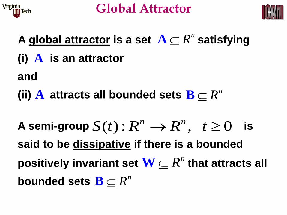
Global Attractor
A global attractor is a set satisfying nRA
(i) is an attractor
and
(ii) attracts all bounded sets
A
A nRB
( ) : , 0 n nS t R R tA semi-group is
said to be dissipative if there is a bounded
positively invariant set that attracts all
bounded sets
nRWnRB
Dissipative System
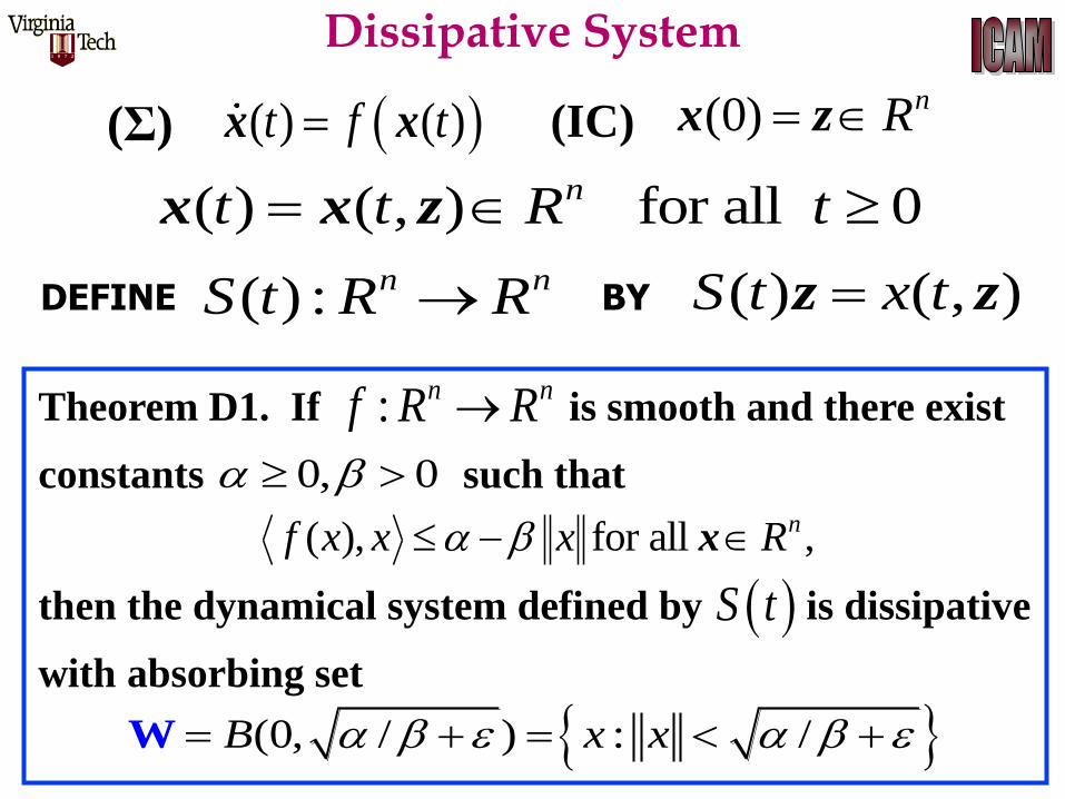
( ) ( , ) for all 0nt t R t x x z
(0) nR x z(IC) ( ) ( )t f tx x(Σ)
( ) ( , )S t x tz z( ) : n nS t R RDEFINE BY
Theorem D1. If is smooth and there exist
constants such that
then the dynamical system defined by is dissipative
with absorbing set
0, 0
S t
(0, / ) : /B x x W
( ), for all , nf x x x Rx
: n nf R R
Dissipative System
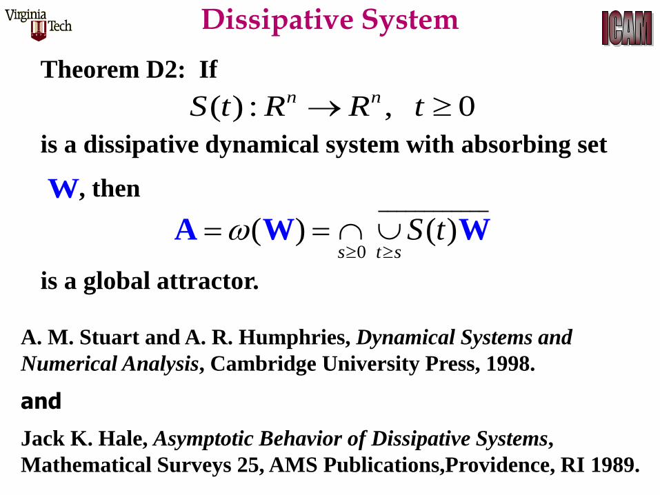
( ) : , 0n nS t R R t
Theorem D2: If
is a dissipative dynamical system with absorbing set
, then
is a global attractor.
W
0( ) ( )
s t sS t
A W W
____________
A. M. Stuart and A. R. Humphries, Dynamical Systems and
Numerical Analysis, Cambridge University Press, 1998.
and
Jack K. Hale, Asymptotic Behavior of Dissipative Systems,
Mathematical Surveys 25, AMS Publications,Providence, RI 1989.
Top Related