


γλώσσες
Σελίδες
Νομικός

Introduction Renormalization Some applications The flow on the lattice
Overview
Introduction
Renormalization
Some applications
The flow on the lattice
2/38
Introduction Renormalization Some applications The flow on the lattice
Summary of conventions
I Mainly concerned with SU(3) Yang-Mills or QCD
S = −1
2g20
∫d4x Tr[FµνFµν ] +
∫d4x
Nf∑i=1
ψi( /D + m)ψi
I The lie algebra su(3) is the linear space of all traceless anti-hermitian 3× 3matrices
I We choose a basis in su(3), Ta with a = 1, . . . , 8 such that
Tr{TaTb} = −δab2
I Greek indices µ, ν, · · · = 0, . . . , 3 run over space-time coordinates, while latinindices run over the spatial coordinates i, j, · · · = 1, 2, 3.
I We abreviate integrals over momenta∫p
=
∫ ∞−∞
d4p(2π)4
3/38
Introduction Renormalization Some applications The flow on the lattice
Yang-Mills gradient flow: basics [Narayanan, Neuberger ’06; Luscher ’10]
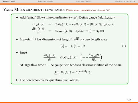
I Add “extra” (flow) time coordinate t (6= x0). Define gauge field Bµ(x, t)
Gνµ(x, t) = ∂νBµ(x, t)− ∂νBµ(x, t) + [Bν(x, t),Bµ(x, t)]dBµ(x, t)
dt= DνGνµ(x, t); Bµ(x, t = 0) = Aµ(x) .
I Important: t has dimensions of length2.√
8t is a new length scale
[x] = −1; [t] = −2 (1)
I SincedBµ(x, t)
dt= DνGνµ(x, t)
(∼ −
δSYM[B]
δBµ
)At large flow time t→∞ gauge field tends to classical solution of the e.o.m.
limt→∞
Bµ(t, x) = Aclassicalµ (x) .
I The flow smooths the quantum fluctuations!
4/38
Introduction Renormalization Some applications The flow on the lattice
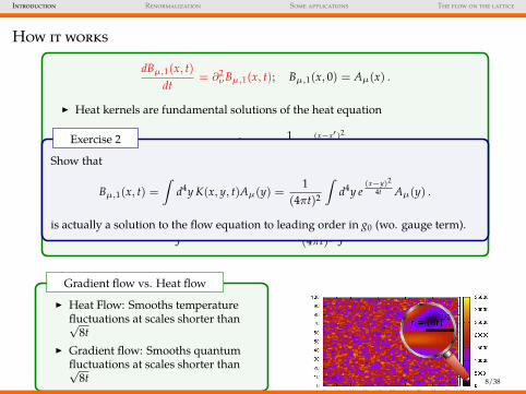
How it works
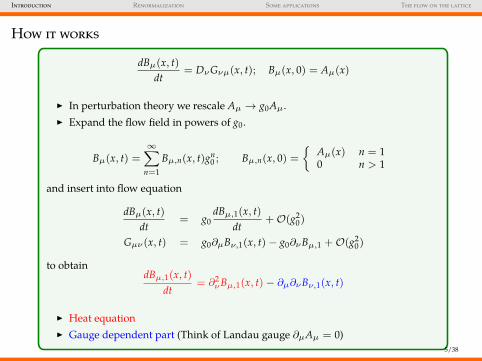
dBµ(x, t)dt
= DνGνµ(x, t); Bµ(x, 0) = Aµ(x)
I In perturbation theory we rescale Aµ → g0Aµ.I Expand the flow field in powers of g0.
Bµ(x, t) =
∞∑n=1
Bµ,n(x, t)gn0 ; Bµ,n(x, 0) =
{Aµ(x) n = 10 n > 1
and insert into flow equation
dBµ(x, t)dt
= g0dBµ,1(x, t)
dt+O(g2
0)
Gµν(x, t) = g0∂µBν,1(x, t)− g0∂νBµ,1 +O(g20)
to obtaindBµ,1(x, t)
dt= ∂2
νBµ,1(x, t)− ∂µ∂νBν,1(x, t)
I Heat equationI Gauge dependent part (Think of Landau gauge ∂µAµ = 0)
5/38
Introduction Renormalization Some applications The flow on the lattice
How it works
dBµ,1(x, t)dt
= ∂2νBµ,1(x, t)− ∂µ∂νBν,1(x, t); Bµ,1(x, 0) = Aµ(x) .
I Linear equation in Bµ,1(x, t)I ∂-operator is “diagonal” in momentum space. Use
Bµ,1(x, t) =
∫p
eıpxBµ,1(p, t)(∫
p≡∫ ∞−∞
d4p(2π)4
)to get
dBµ,1(x, t)dt
=
∫p
dBµ,1(p, t)dt
eıpx
∂2νBµ,1(x, t)− ∂µ∂νBν,1(x, t) = −
∫p
p2Bµ,1(p, t)eıpx +
∫p
pµpν Bν,1(p, t)eıpx
Flow equation in momentum space
dBµ,1(p, t)dt
= −(
p2δµν − pµpν)
Bν,1(p, t); Bµ,1(p, 0) = Aµ(p) .
6/38
Introduction Renormalization Some applications The flow on the lattice
How it works
dBµ,1(p, t)dt
= −(
p2δµν − pµpν)
Bν,1(p, t); Bµ,1(p, 0) = Aµ(p) .
Forget about gauge terms: Solution
Bµ,1(p, t) = e−tp2Bµ,1(p, 0) = e−tp2
Aµ(p)
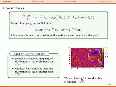
High momentum modes (small scale fluctuations) are exponentially damped
I Heat Flow: Smooths temperaturefluctuations at scales shorter than√
8tI Gradient flow: Smooths quantum
fluctuations at scales shorter than√8t
Gradient flow vs. Heat flow
We are “looking” at world with aresolution ∼
√8t.
7/38
Introduction Renormalization Some applications The flow on the lattice
How it works
dBµ,1(p, t)dt
= −(
p2δµν − pµpν)
Bν,1(p, t); Bµ,1(p, 0) = Aµ(p) .
Forget about gauge terms: Solution
Bµ,1(p, t) = e−tp2Bµ,1(p, 0) = e−tp2
Aµ(p)
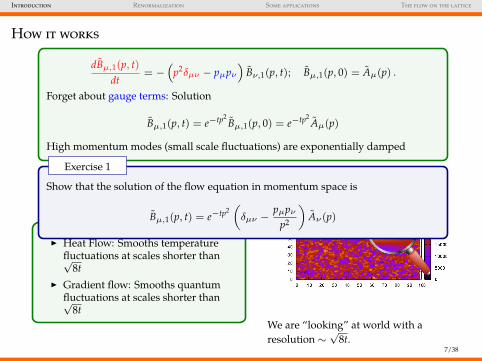
High momentum modes (small scale fluctuations) are exponentially damped
I Heat Flow: Smooths temperaturefluctuations at scales shorter than√
8tI Gradient flow: Smooths quantum
fluctuations at scales shorter than√8t
Gradient flow vs. Heat flow
We are “looking” at world with aresolution ∼
√8t.
Show that the solution of the flow equation in momentum space is
Bµ,1(p, t) = e−tp2(δµν −
pµpνp2
)Aν(p)
Exercise 1
7/38
Introduction Renormalization Some applications The flow on the lattice
How it works
dBµ,1(x, t)dt
= ∂2νBµ,1(x, t); Bµ,1(x, 0) = Aµ(x) .
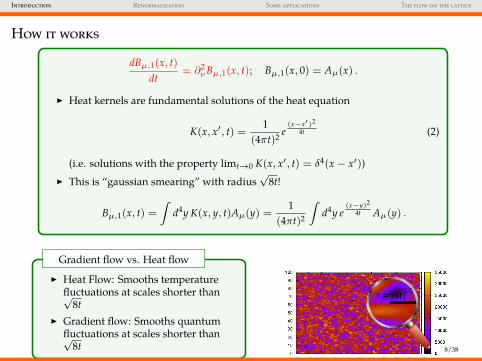
I Heat kernels are fundamental solutions of the heat equation
K(x, x′, t) =1
(4πt)2 e(x−x′)2
4t (2)
(i.e. solutions with the property limt→0 K(x, x′, t) = δ4(x − x′))I This is “gaussian smearing” with radius
√8t!
Bµ,1(x, t) =
∫d4y K(x, y, t)Aµ(y) =
1(4πt)2
∫d4y e
(x−y)24t Aµ(y) .
I Heat Flow: Smooths temperaturefluctuations at scales shorter than√
8tI Gradient flow: Smooths quantum
fluctuations at scales shorter than√8t
Gradient flow vs. Heat flow
We are “looking” at world with aresolution ∼
√8t.
8/38
Introduction Renormalization Some applications The flow on the lattice
How it works
dBµ,1(x, t)dt
= ∂2νBµ,1(x, t); Bµ,1(x, 0) = Aµ(x) .
I Heat kernels are fundamental solutions of the heat equation
K(x, x′, t) =1
(4πt)2 e(x−x′)2
4t (2)
(i.e. solutions with the property limt→0 K(x, x′, t) = δ4(x − x′))I This is “gaussian smearing” with radius
√8t!
Bµ,1(x, t) =
∫d4y K(x, y, t)Aµ(y) =
1(4πt)2
∫d4y e
(x−y)24t Aµ(y) .
I Heat Flow: Smooths temperaturefluctuations at scales shorter than√
8tI Gradient flow: Smooths quantum
fluctuations at scales shorter than√8t
Gradient flow vs. Heat flow
We are “looking” at world with aresolution ∼
√8t.
Show that
Bµ,1(x, t) =
∫d4y K(x, y, t)Aµ(y) =
1(4πt)2
∫d4y e
(x−y)24t Aµ(y) .
is actually a solution to the flow equation to leading order in g0 (wo. gauge term).
Exercise 2
8/38
Introduction Renormalization Some applications The flow on the lattice
Main characteristic of the flowI Gauge covariant under gauge transformations that are independent of t
dBµ(x, t)dt
= DνGνµ(x, t)
I Composite gauge invariant operators are renormalized observables defined ata scale µ = 1/
√8t [M. Luscher ’10; M. Luscher, P. Weisz ’11].
I Example (Note that at t = 0 this is terribly divergent ∝ 1/a4)
〈E(t)〉 = −12〈TrGµν(x, t)Gµν(x, t)〉
finite quantity for t > 0.I Continuum limit to be taken at fixed t.I The energy density 〈E(t)〉will be a main character in this talk!!
9/38
Introduction Renormalization Some applications The flow on the lattice
Main characteristic of the flowI Gauge covariant under gauge transformations that are independent of t
dBµ(x, t)dt
= DνGνµ(x, t)
I Composite gauge invariant operators are renormalized observables defined ata scale µ = 1/
√8t [M. Luscher ’10; M. Luscher, P. Weisz ’11].
I Example (Note that at t = 0 this is terribly divergent ∝ 1/a4)
〈E(t)〉 = −12〈TrGµν(x, t)Gµν(x, t)〉
finite quantity for t > 0.I Continuum limit to be taken at fixed t.I The energy density 〈E(t)〉will be a main character in this talk!!
Show that the flow equation is gauge covariant
Exercise 3
9/38
Introduction Renormalization Some applications The flow on the lattice
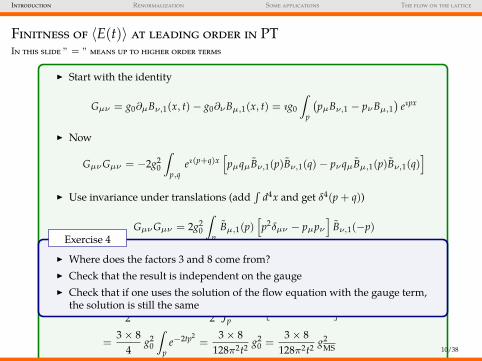
Finitness of 〈E(t)〉 at leading order in PTIn this slide ” = ” means up to higher order terms
I Start with the identity
Gµν = g0∂µBν,1(x, t)− g0∂νBµ,1(x, t) = ıg0
∫p
(pµBν,1 − pνBµ,1
)eıpx
I Now
GµνGµν = −2g20
∫p,q
eı(p+q)x[pµqµBν,1(p)Bν,1(q)− pνqµBµ,1(p)Bν,1(q)
]I Use invariance under translations (add
∫d4x and get δ4(p + q))
GµνGµν = 2g20
∫p
Bµ,1(p)[p2δµν − pµpν
]Bν,1(−p)
I Use the solution of the flow equation and gluon propagator〈Aaµ(p)Ab
ν(−p)〉 =δabp2 δµν
〈E(t)〉 = −12〈TrGµνGµν〉 =
g202
∫p
e−2tp2 [p2δµν − pµpν
]〈Tr{Aµ(p)Aν(−p)}〉
=3× 8
4g2
0
∫p
e−2tp2=
3× 8128π2t2
g20 =
3× 8128π2t2
g2MS 10/38
Introduction Renormalization Some applications The flow on the lattice
Finitness of 〈E(t)〉 at leading order in PTIn this slide ” = ” means up to higher order terms
I Start with the identity
Gµν = g0∂µBν,1(x, t)− g0∂νBµ,1(x, t) = ıg0
∫p
(pµBν,1 − pνBµ,1
)eıpx
I Now
GµνGµν = −2g20
∫p,q
eı(p+q)x[pµqµBν,1(p)Bν,1(q)− pνqµBµ,1(p)Bν,1(q)
]I Use invariance under translations (add
∫d4x and get δ4(p + q))
GµνGµν = 2g20
∫p
Bµ,1(p)[p2δµν − pµpν
]Bν,1(−p)
I Use the solution of the flow equation and gluon propagator〈Aaµ(p)Ab
ν(−p)〉 =δabp2 δµν
〈E(t)〉 = −12〈TrGµνGµν〉 =
g202
∫p
e−2tp2 [p2δµν − pµpν
]〈Tr{Aµ(p)Aν(−p)}〉
=3× 8
4g2
0
∫p
e−2tp2=
3× 8128π2t2
g20 =
3× 8128π2t2
g2MS
I Where does the factors 3 and 8 come from?I Check that the result is independent on the gaugeI Check that if one uses the solution of the flow equation with the gauge term,
the solution is still the same
Exercise 4
10/38
Introduction Renormalization Some applications The flow on the lattice
Scale setting and renormalized couplings
0 0.02 0.04 0.06 0.08 0.1 0.12 0.14 0.16 0.18 0.2
t /r02
0
0.1
0.2
0.3
0.4
0.5
t2⟨E⟩
t0
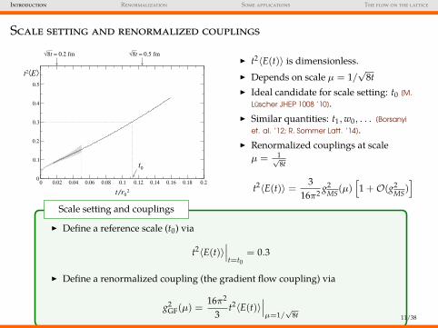
√ 8t = 0.2 fm √ 8t = 0.5 fmI t2〈E(t)〉 is dimensionless.I Depends on scale µ = 1/
√8t
I Ideal candidate for scale setting: t0 [M.Luscher JHEP 1008 ’10].
I Similar quantities: t1,w0, . . . [Borsanyiet. al. ’12; R. Sommer Latt. ’14].
I Renormalized couplings at scaleµ = 1√
8t
t2〈E(t)〉 =3
16π2 g2MS(µ)
[1 +O(g2
MS)]
I Define a reference scale (t0) via
t2〈E(t)〉∣∣∣t=t0
= 0.3
I Define a renormalized coupling (the gradient flow coupling) via
g2GF(µ) =
16π2
3t2〈E(t)〉
∣∣∣µ=1/
√8t
Scale setting and couplings
11/38
Introduction Renormalization Some applications The flow on the lattice
Scale setting and renormalized couplings
0 0.02 0.04 0.06 0.08 0.1 0.12 0.14 0.16 0.18 0.2
t /r02
0
0.1
0.2
0.3
0.4
0.5
t2⟨E⟩
t0
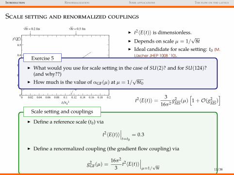
√ 8t = 0.2 fm √ 8t = 0.5 fmI t2〈E(t)〉 is dimensionless.I Depends on scale µ = 1/
√8t
I Ideal candidate for scale setting: t0 [M.Luscher JHEP 1008 ’10].
I Similar quantities: t1,w0, . . . [Borsanyiet. al. ’12; R. Sommer Latt. ’14].
I Renormalized couplings at scaleµ = 1√
8t
t2〈E(t)〉 =3
16π2 g2MS(µ)
[1 +O(g2
MS)]
I Define a reference scale (t0) via
t2〈E(t)〉∣∣∣t=t0
= 0.3
I Define a renormalized coupling (the gradient flow coupling) via
g2GF(µ) =
16π2
3t2〈E(t)〉
∣∣∣µ=1/
√8t
Scale setting and couplings
I What would you use for scale setting in the case of SU(2)? and for SU(124)?(and why??)
I How much is the value of αGF(µ) at µ = 1/√
8t0
Exercise 5
11/38
Introduction Renormalization Some applications The flow on the lattice
Exercises of the introduction
1. Show that the solution of the flow equation in momentum space is
Bµ,1(p, t) = e−tp2(δµν −
pµpνp2
)Aν(p)
2. Show that
Bµ,1(x, t) =
∫d4y K(x, y, t)Aµ(y) =
1(4πt)2
∫d4y e
(x−y)24t Aµ(y) .
is actually a solution to the flow equation to leading order in g0 (wo. gaugeterm).
3. Show that the flow equation is gauge covariant4. In the formula for 〈E(t)〉 to leading order
I Where does the factors 3 and 8 come from?I Check that the result is independent on the gaugeI Check that if one uses the solution of the flow equation with the gauge term, the
solution is still the same5. Scale setting and couplings
I What would you use for scale setting in the case of SU(2)? and for SU(124)? (andwhy??)
I How much is the value of αGF(µ) at µ = 1/√
8t0
12/38
Introduction Renormalization Some applications The flow on the lattice
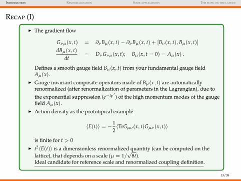
Recap (I)I The gradient flow
Gνµ(x, t) = ∂νBµ(x, t)− ∂νBµ(x, t) + [Bν(x, t),Bµ(x, t)]dBµ(x, t)
dt= DνGνµ(x, t); Bµ(x, t = 0) = Aµ(x) .
Defines a smooth gauge field Bµ(x, t) from your fundamental gauge fieldAµ(x).
I Gauge invariant composite operators made of Bµ(x, t) are automaticallyrenormalized (after renormalization of parameters in the Lagrangian), due tothe exponential suppression (e−tp2 ) of the high momentum modes of the gaugefield Aµ(x).
I Action density as the prototipical example
〈E(t)〉 = −12〈TrGµν(x, t)Gµν(x, t)〉
is finite for t > 0I t2〈E(t)〉 is a dimensionless renormalized quantity (can be computed on the
lattice), that depends on a scale (µ = 1/√
8t).Ideal candidate for reference scale and renormalized coupling definition.
13/38
Introduction Renormalization Some applications The flow on the lattice
Overview
Introduction
Renormalization
Some applications
The flow on the lattice
14/38
Introduction Renormalization Some applications The flow on the lattice
Beyond leading order
I An explicit calculation shows that actually t2〈E(t)〉 is finite to NLO [Luscher ’10]
t2〈E(t)〉 =3
16π2 g2MS(µ)
[1 + c1g2
MS(µ) +O(g4MS)]
with c1 finiteI Actually this is true to all orders, and for all gauge invariant observables made
of the flow field Bµ(x, t) [Luscher, Weisz ’11]
I How to prove this? We know how to renormalize composite operators, but...I Bµ(x, t) is not a local field (i.e. Bµ(x, t) depends on the fundamental field Aµ(y)
for y 6= x)!I One has to see the the flow field Bµ(x, t) as living in 5d!!
15/38
Introduction Renormalization Some applications The flow on the lattice
5d local formulation [Zinn-Justin ’86, Zwanziger ’88, Luscher, Weisz ’11]
Usually one sees the gradient flow observables in “two steps”
〈O[Bµ]〉 =1Z
∫DA O[Bµ]e−SYM[Aµ]
where Bµ is the solution of the flow equation
dBµ(x, t)dt
= DνGνµ(x, t); Bµ(x, t = 0) = Aµ(x) .
Alternatively, we can promote t ∈ (0,∞) to a fifth coordinate and set-up a weird 5dtheory
Z =
∫DBµDLµ e−S5d[Bµ,Lµ]
with S5d = SYM + Sbulk
SYM = −1
2g20
∫d4x Tr[FµνFµν ]
Sbulk = −2∫ ∞
0dt∫
d4xTr {Lµ(x, t) [∂tBµ − DνGνµ]}
16/38
Introduction Renormalization Some applications The flow on the lattice
5d local formulation [Zinn-Justin ’86, Zwanziger ’88, Luscher, Weisz ’11]
Z =
∫DBµDLµ e−S5d[Bµ,Lµ]; S5d = SYM + Sbulk
SYM = −1
2g20
∫d4x Tr[FµνFµν ]
Sbulk = −2∫ ∞
0dt∫
d4xTr {Lµ(x, t) [∂tBµ − DνGνµ]}
I Lµ(x, t) = Laµ(x, t)Ta lives in the adjoint representation, with purely imaginary
componentsI The path integral DLµ can be done exactly∫
DLµe−Sbulk = δ (∂tBµ − DνGνµ) ,
and it imposes the flow equationI Now we have
〈O[Bµ]〉 =1Z
∫DBDL O[Bµ]e−S5d[Bµ,Lµ] =
∫DB O[Bµ]e−SYM[Aµ]δ (∂tBµ − DνGνµ) ,
17/38
Introduction Renormalization Some applications The flow on the lattice
5d local formulation [Zinn-Justin ’86, Zwanziger ’88, Luscher, Weisz ’11]
Z =
∫DBµDLµ e−S5d[Bµ,Lµ]; S5d = SYM + Sbulk
SYM = −1
2g20
∫d4x Tr[FµνFµν ]
Sbulk = −2∫ ∞
0dt∫
d4xTr {Lµ(x, t) [∂tBµ − DνGνµ]}
I Lµ(x, t) = Laµ(x, t)Ta lives in the adjoint representation, with purely imaginary
componentsI The path integral DLµ can be done exactly∫
DLµe−Sbulk = δ (∂tBµ − DνGνµ) ,
and it imposes the flow equationI Now we have
〈O[Bµ]〉 =1Z
∫DBDL O[Bµ]e−S5d[Bµ,Lµ] =
∫DB O[Bµ]e−SYM[Aµ]δ (∂tBµ − DνGνµ) ,
I What are the dimensions of the field Lµ(x, t)?I Name a few symmetries of the action S5d
Exercise 6
17/38
Introduction Renormalization Some applications The flow on the lattice
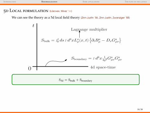
5d Local formulation [Luscher, Weisz ’11]
We can see the theory as a 5d local field theory [Zinn-Justin ’86, Zinn-Justin, Zwanziger ’88]
Sbulk =∫ t0 ds
∫d4xLa
µ(x, t){∂tB
aµ −DνG
aµν
}
Sboundary =∫d4x 1
4g2Ga
µνGaµν
0
tLagrange multiplier
4d space-time
S5d = Sbulk + Sboundary
18/38
Introduction Renormalization Some applications The flow on the lattice
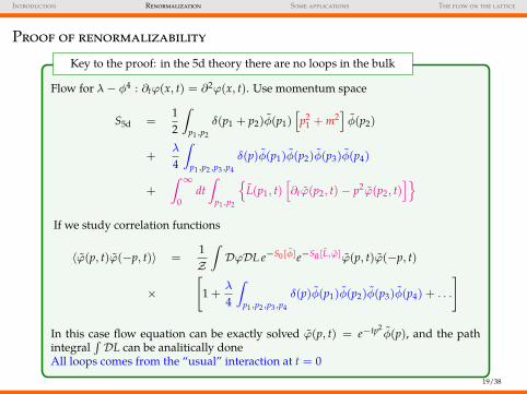
Proof of renormalizability
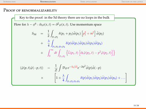
Flow for λ− φ4 : ∂tϕ(x, t) = ∂2ϕ(x, t). Use momentum space
S5d =12
∫p1,p2
δ(p1 + p2)φ(p1)[p2
1 + m2]φ(p2)
+λ
4
∫p1,p2,p3,p4
δ(p)φ(p1)φ(p2)φ(p3)φ(p4)
+
∫ ∞0
dt∫
p1,p2
{L(p1, t)
[∂tϕ(p2, t)− p2ϕ(p2, t)
]}If we study correlation functions
〈ϕ(p, t)ϕ(−p, t)〉 =1Z
∫DϕDL e−S0[φ]e−Sfl[L,ϕ]ϕ(p, t)ϕ(−p, t)
×[
1 +λ
4
∫p1,p2,p3,p4
δ(p)φ(p1)φ(p2)φ(p3)φ(p4) + . . .
]
In this case flow equation can be exactly solved ϕ(p, t) = e−tp2φ(p), and the path
integral∫DL can be analitically done
All loops comes from the “usual” interaction at t = 0
Key to the proof: in the 5d theory there are no loops in the bulk
19/38
Introduction Renormalization Some applications The flow on the lattice
Proof of renormalizability
Flow for λ− φ4 : ∂tϕ(x, t) = ∂2ϕ(x, t). Use momentum space
S5d =12
∫p1,p2
δ(p1 + p2)φ(p1)[p2
1 + m2]φ(p2)
+λ
4
∫p1,p2,p3,p4
δ(p)φ(p1)φ(p2)φ(p3)φ(p4)
+
∫ ∞0
dt∫
p1,p2
{L(p1, t)
[∂tϕ(p2, t)− p2ϕ(p2, t)
]}
〈ϕ(p, t)ϕ(−p, t)〉 =1Z
∫Dϕ e−S0[φ]e−2tp2
φ(p)φ(−p)
×[
1 +λ
4
∫p1,p2,p3,p4
δ(p)φ(p1)φ(p2)φ(p3)φ(p4) + . . .
]
Key to the proof: in the 5d theory there are no loops in the bulk
19/38
Introduction Renormalization Some applications The flow on the lattice
Proof of renormalizability
Flow for λ− φ4 : ∂tϕ(x, t) = ∂2ϕ(x, t). Use momentum space
S5d =12
∫p1,p2
δ(p1 + p2)φ(p1)[p2
1 + m2]φ(p2)
+λ
4
∫p1,p2,p3,p4
δ(p)φ(p1)φ(p2)φ(p3)φ(p4)
+
∫ ∞0
dt∫
p1,p2
{L(p1, t)
[∂tϕ(p2, t)− p2ϕ(p2, t)
]}
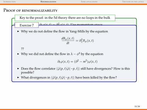
Key to the proof: in the 5d theory there are no loops in the bulk
I Why we do not define the flow in Yang-Mills by the equation
dBµ(x, t)dt
= ∂2νBµ(x, t)
??I Why we did not define the flow in λ− φ4 by the equation
∂tϕ(x, t) = (∂2 − m2)ϕ(x, t)
I Does the flow correlator 〈ϕ(p, t)ϕ(−p, t)〉 still have divergences? How is thispossible?
I What divergences in 〈ϕ(p, t)ϕ(−p, t)〉 have been killed by the flow?
Exercise 7
19/38
Introduction Renormalization Some applications The flow on the lattice
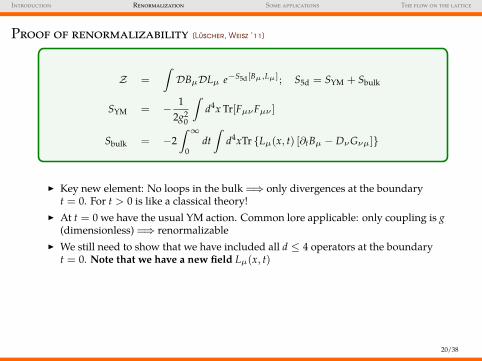
Proof of renormalizability [Luscher, Weisz ’11]
Z =
∫DBµDLµ e−S5d[Bµ,Lµ]; S5d = SYM + Sbulk
SYM = −1
2g20
∫d4x Tr[FµνFµν ]
Sbulk = −2∫ ∞
0dt∫
d4xTr {Lµ(x, t) [∂tBµ − DνGνµ]}
I Key new element: No loops in the bulk =⇒ only divergences at the boundaryt = 0. For t > 0 is like a classical theory!
I At t = 0 we have the usual YM action. Common lore applicable: only coupling is g(dimensionless) =⇒ renormalizable
I We still need to show that we have included all d ≤ 4 operators at the boundaryt = 0. Note that we have a new field Lµ(x, t)
20/38
Introduction Renormalization Some applications The flow on the lattice
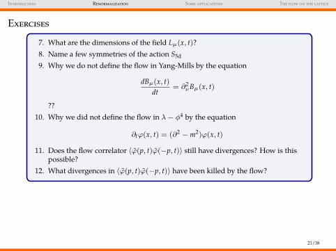
Exercises
7. What are the dimensions of the field Lµ(x, t)?8. Name a few symmetries of the action S5d
9. Why we do not define the flow in Yang-Mills by the equation
dBµ(x, t)dt
= ∂2νBµ(x, t)
??10. Why we did not define the flow in λ− φ4 by the equation
∂tϕ(x, t) = (∂2 − m2)ϕ(x, t)
11. Does the flow correlator 〈ϕ(p, t)ϕ(−p, t)〉 still have divergences? How is thispossible?
12. What divergences in 〈ϕ(p, t)ϕ(−p, t)〉 have been killed by the flow?
21/38
Introduction Renormalization Some applications The flow on the lattice
Recap (II)I The Yang-Mills flow can be seen as a 5d local quantum field theory.I The flow equation is imposed by adding “Lagrange multipliers” fields Lµ(x, t).
The path integral over Lµ(x, t) gives a delta function.I Usual tools of quantum field theory can be applied to this theory.I Very similar to stochastic quantization [Book by Zinn-Justin]
22/38
Introduction Renormalization Some applications The flow on the lattice
Overview
Introduction
Renormalization
Some applications
The flow on the lattice
23/38
Introduction Renormalization Some applications The flow on the lattice
Scale setting
0 0.02 0.04 0.06 0.08 0.1 0.12 0.14 0.16 0.18 0.2
t /r02
0
0.1
0.2
0.3
0.4
0.5
t2⟨E⟩
t0
√ 8t = 0.2 fm √ 8t = 0.5 fm
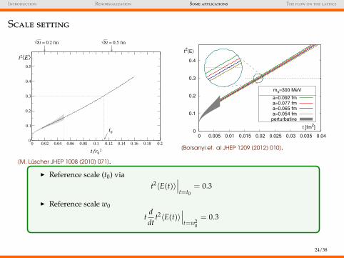
[M. Luscher JHEP 1008 (2010) 071].
0
0.1
0.2
0.3
0.4
0 0.005 0.01 0.015 0.02 0.025 0.03 0.035 0.04
t2⟨E⟩
t [fm2]
mπ≈300 MeV
a≈0.092 fma≈0.077 fma≈0.065 fma≈0.054 fm
perturbative
[Borsanyi et. al JHEP 1209 (2012) 010].
I Reference scale (t0) viat2〈E(t)〉
∣∣∣t=t0
= 0.3
I Reference scale w0
tddt
t2〈E(t)〉∣∣∣t=w2
0= 0.3
24/38
Introduction Renormalization Some applications The flow on the lattice
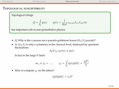
Topological susceptibility
Topological charge
Q =
∫x
q(x); q(x) =1
32π2 εµνρσFµνFρσ(x)
has important role in non-perturbative physics
I Q: Why is the η meson not a pseudo-goldstone boson (UA(1) puzzle)?I A: UA(1) is only a symmetry at the classical level, destroyed by quantum
fluctuations∂µψγµγ5ψ(x) ∝ q(x) .
In fact in the large N limit
mη ∝ χt + . . . ; χt =
∫x〈q(x)q(0)〉 =
〈Q2〉V
I How to compute χt on the lattice?
〈q(0)q(0)〉 ∼ 1/a4
25/38
Introduction Renormalization Some applications The flow on the lattice
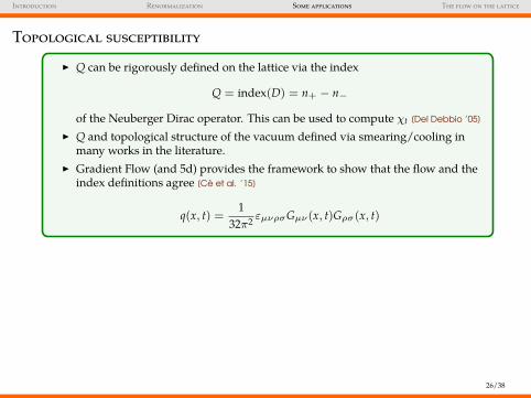
Topological susceptibilityI Q can be rigorously defined on the lattice via the index
Q = index(D) = n+ − n−
of the Neuberger Dirac operator. This can be used to compute χt [Del Debbio ’05]
I Q and topological structure of the vacuum defined via smearing/cooling inmany works in the literature.
I Gradient Flow (and 5d) provides the framework to show that the flow and theindex definitions agree [Ce et al. ’15]
q(x, t) =1
32π2 εµνρσGµν(x, t)Gρσ(x, t)
26/38
Introduction Renormalization Some applications The flow on the lattice
Running couplingsI Use the gradient flow coupling definition in finite volume
α(µ) = #t2〈E(t)〉∣∣∣µ=1/
√8t=1/(cL)
Constant # depends on the choice of boundary conditions (periodic, twisted,dirichlet (SF), . . . )
I We can measure how much changes the coupling when we change µ→ µ/2 bychanging our lattice size L
I Step scaling functionσ(u) = α(µ/2)
∣∣∣α(µ)=u
27/38
Introduction Renormalization Some applications The flow on the lattice
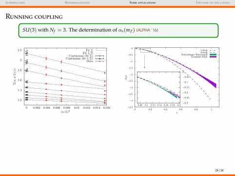
Running coupling
SU(3) with Nf = 3. The determination of αs(mZ) [ALPHA ’16]
1.2
1.4
1.6
1.8
2
2.2
0 0.002 0.004 0.006 0.008 0.01 0.012 0.014 0.016
Σ(u,a/L
)/u
(a/L)2
Fit ΣFit 1/Σ
Continuum (fit Σ)Continuum (fit 1/Σ)
Data
−4.5
−4
−3.5
−3
−2.5
−2
−1.5
−1
−0.5
0
0 0.2 0.4 0.6 0.8 1
β(g)
α
1-loop2-loop
Schrödinger FunctionalGradient Flow
0.08 0.1 0.12 0.14 0.16 0.18 0.2−0.3
−0.25
−0.2
−0.15
−0.1
−0.05
0
28/38
Introduction Renormalization Some applications The flow on the lattice
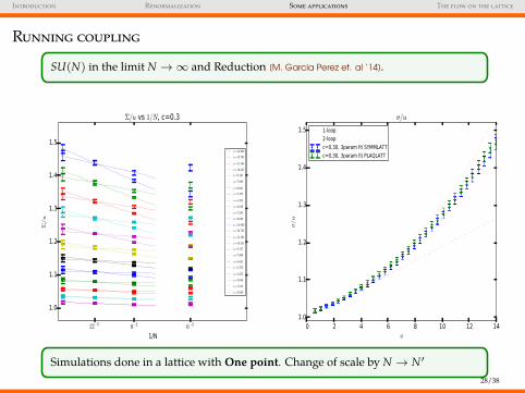
Running coupling
SU(N) in the limit N →∞ and Reduction [M. Garcia Perez et. al ’14].
6−28−212−2
1/N
1.0
1.1
1.2
1.3
1.4
1.5
Σ/u
Σ/u vs 1/N, c=0.3
u=14.000
u=12.782
u=11.564
u=10.345
u=9.127
u=7.909
u=6.691
u=5.473
u=4.255
u=3.036
u=1.818
u=0.600
u=14.000
u=12.782
u=11.564
u=10.345
u=9.127
u=7.909
u=6.691
u=5.473
u=4.255
u=3.036
u=1.818
u=0.600
0 2 4 6 8 10 12 14u
1.0
1.1
1.2
1.3
1.4
1.5
σ/u
σ/u
1-loop2-loopc=0.30, 3param fit SYMMLATTc=0.30, 3param fit PLAQLATT
Simulations done in a lattice with One point. Change of scale by N → N′
28/38
Introduction Renormalization Some applications The flow on the lattice
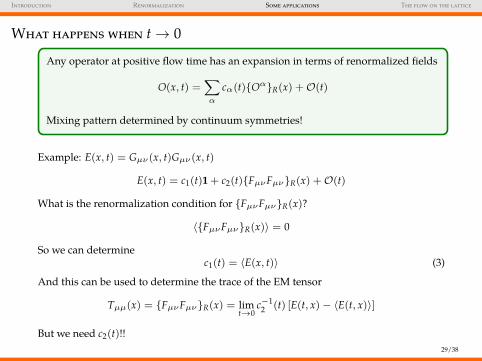
What happens when t → 0
Any operator at positive flow time has an expansion in terms of renormalized fields
O(x, t) =∑α
cα(t){Oα}R(x) +O(t)
Mixing pattern determined by continuum symmetries!
Example: E(x, t) = Gµν(x, t)Gµν(x, t)
E(x, t) = c1(t)1 + c2(t){FµνFµν}R(x) +O(t)
What is the renormalization condition for {FµνFµν}R(x)?
〈{FµνFµν}R(x)〉 = 0
So we can determinec1(t) = 〈E(x, t)〉 (3)
And this can be used to determine the trace of the EM tensor
Tµµ(x) = {FµνFµν}R(x) = limt→0
c−12 (t) [E(t, x)− 〈E(t, x)〉]
But we need c2(t)!!29/38
Introduction Renormalization Some applications The flow on the lattice
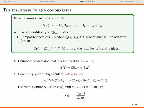
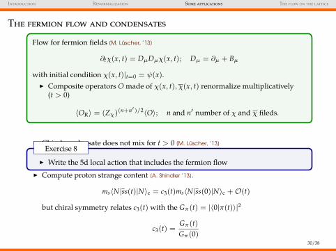
The fermion flow and condensates
Flow for fermion fields [M. Luscher, ’13]
∂tχ(x, t) = DµDµχ(x, t); Dµ = ∂µ + Bµ
with initial condition χ(x, t)|t=0 = ψ(x).I Composite operators O made of χ(x, t), χ(x, t) renormalize multiplicatively
(t > 0)
〈OR〉 = (Zχ)(n+n′)/2〈O〉; n and n′ number of χ and χ fileds.
I Chiral condensate does not mix for t > 0 [M. Luscher, ’13]
Σ(t) = 〈u(t, x)u(t, x)〉
I Compute proton strange content [A. Shindler ’13].
ms〈N|ss(t)|N〉c = c3(t)ms〈N|ss(0)|N〉c +O(t)
but chiral symmetry relates c3(t) with the Gπ(t) = |〈0|π(t)〉|2
c3(t) =Gπ(t)Gπ(0)
30/38
Introduction Renormalization Some applications The flow on the lattice
The fermion flow and condensates
Flow for fermion fields [M. Luscher, ’13]
∂tχ(x, t) = DµDµχ(x, t); Dµ = ∂µ + Bµ
with initial condition χ(x, t)|t=0 = ψ(x).I Composite operators O made of χ(x, t), χ(x, t) renormalize multiplicatively
(t > 0)
〈OR〉 = (Zχ)(n+n′)/2〈O〉; n and n′ number of χ and χ fileds.
I Chiral condensate does not mix for t > 0 [M. Luscher, ’13]
Σ(t) = 〈u(t, x)u(t, x)〉
I Compute proton strange content [A. Shindler ’13].
ms〈N|ss(t)|N〉c = c3(t)ms〈N|ss(0)|N〉c +O(t)
but chiral symmetry relates c3(t) with the Gπ(t) = |〈0|π(t)〉|2
c3(t) =Gπ(t)Gπ(0)
I Write the 5d local action that includes the fermion flow
Exercise 8
30/38
Introduction Renormalization Some applications The flow on the lattice
Overview
Introduction
Renormalization
Some applications
The flow on the lattice
31/38
Introduction Renormalization Some applications The flow on the lattice
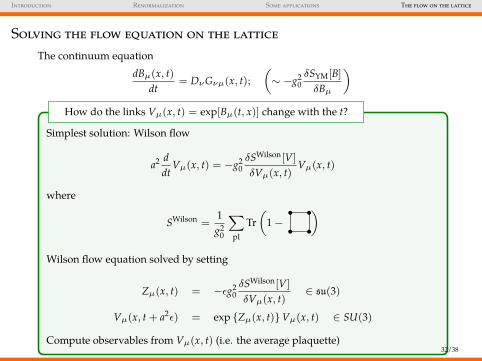
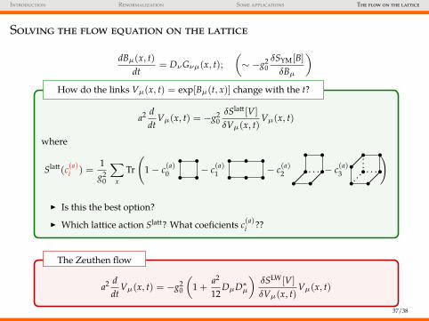
Solving the flow equation on the latticeThe continuum equation
dBµ(x, t)dt
= DνGνµ(x, t);(∼ −g2
0δSYM[B]
δBµ
)
Simplest solution: Wilson flow
a2 ddt
Vµ(x, t) = −g20δSWilson[V]
δVµ(x, t)Vµ(x, t)
where
SWilson =1g2
0
∑pl
Tr(
1− rr rr)Wilson flow equation solved by setting
Zµ(x, t) = −εg20δSWilson[V]
δVµ(x, t)∈ su(3)
Vµ(x, t + a2ε) = exp {Zµ(x, t)}Vµ(x, t) ∈ SU(3)
Compute observables from Vµ(x, t) (i.e. the average plaquette)
How do the links Vµ(x, t) = exp[Bµ(t, x)] change with the t?
32/38
Introduction Renormalization Some applications The flow on the lattice
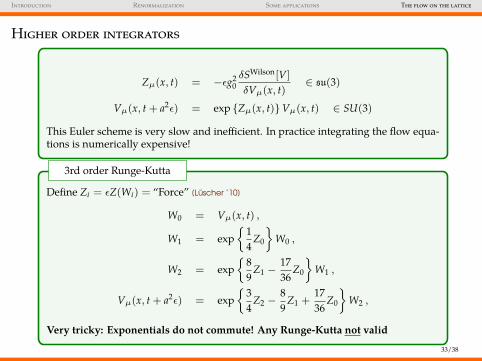
Higher order integrators
Zµ(x, t) = −εg20δSWilson[V]
δVµ(x, t)∈ su(3)
Vµ(x, t + a2ε) = exp {Zµ(x, t)}Vµ(x, t) ∈ SU(3)
This Euler scheme is very slow and inefficient. In practice integrating the flow equa-tions is numerically expensive!
Define Zi = εZ(Wi) = “Force” [Luscher ’10]
W0 = Vµ(x, t) ,
W1 = exp{
14
Z0
}W0 ,
W2 = exp{
89
Z1 −1736
Z0
}W1 ,
Vµ(x, t + a2ε) = exp{
34
Z2 −89
Z1 +1736
Z0
}W2 ,
Very tricky: Exponentials do not commute! Any Runge-Kutta not valid
3rd order Runge-Kutta
33/38
Introduction Renormalization Some applications The flow on the lattice
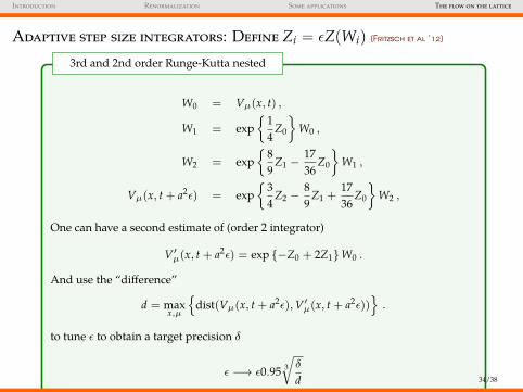
Adaptive step size integrators: Define Zi = εZ(Wi) [Fritzsch et al ’12]
W0 = Vµ(x, t) ,
W1 = exp{
14
Z0
}W0 ,
W2 = exp{
89
Z1 −1736
Z0
}W1 ,
Vµ(x, t + a2ε) = exp{
34
Z2 −89
Z1 +1736
Z0
}W2 ,
One can have a second estimate of (order 2 integrator)
V′µ(x, t + a2ε) = exp {−Z0 + 2Z1}W0 .
And use the “difference”
d = maxx,µ
{dist(Vµ(x, t + a2ε),V′µ(x, t + a2ε))
}.
to tune ε to obtain a target precision δ
ε −→ ε0.95 3√δ
d
3rd and 2nd order Runge-Kutta nested
34/38
Introduction Renormalization Some applications The flow on the lattice
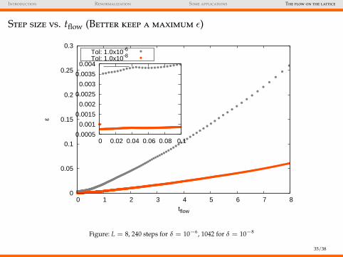
Step size vs. tflow (Better keep a maximum ε)
0
0.05
0.1
0.15
0.2
0.25
0.3
0 1 2 3 4 5 6 7 8
ε
tflow
Tol: 1.0x10⁻⁶
Tol: 1.0x10⁻⁸
0.0005
0.001
0.0015
0.002
0.0025
0.003
0.0035
0.004
0 0.02 0.04 0.06 0.08 0.1
Figure: L = 8, 240 steps for δ = 10−6, 1042 for δ = 10−8
35/38
Introduction Renormalization Some applications The flow on the lattice
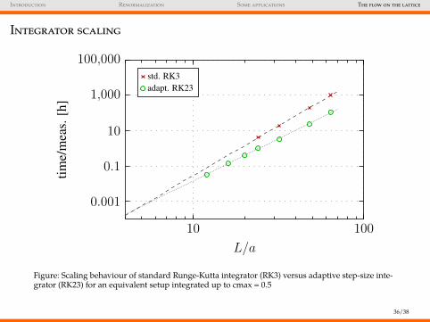
Integrator scaling
10 100
0.001
0.1
10
1,000
100,000
L/a
time/
mea
s.[h
]std. RK3adapt. RK23
Figure: Scaling behaviour of standard Runge-Kutta integrator (RK3) versus adaptive step-size inte-grator (RK23) for an equivalent setup integrated up to cmax = 0.5
36/38
Introduction Renormalization Some applications The flow on the lattice
Solving the flow equation on the lattice
dBµ(x, t)dt
= DνGνµ(x, t);(∼ −g2
0δSYM[B]
δBµ
)
a2 ddt
Vµ(x, t) = −g20δSlatt[V]
δVµ(x, t)Vµ(x, t)
where
Slatt(c(a)i ) =
1g2
0
∑x
Tr
(1− c(a)
0 rr rr− c(a)1 r r rr r r
− c(a)2
�� ��r rr r
r rp p p p − c(a)3
��
��pr r rr rr rp p p ppppppppp
)
I Is this the best option?
I Which lattice action Slatt? What coeficients c(a)i ??
How do the links Vµ(x, t) = exp[Bµ(t, x)] change with the t?
a2 ddt
Vµ(x, t) = −g20
(1 +
a2
12DµD∗µ
)δSLW[V]
δVµ(x, t)Vµ(x, t)
The Zeuthen flow
37/38
Introduction Renormalization Some applications The flow on the lattice
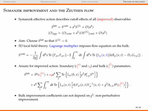
Symanzik improvement and the Zeuthen flow
I Symanzik effective action describes cutoff effects of all (improved) observables
Slatt = Scont + a2S(2) +O(a4)
〈O〉latt = 〈O〉cont + a2〈OS(2)〉cont +O(a4)
I Aim: Choose Slatt so that S(2) = 0.I 5D local field theory. Lagrange multiplier imposes flow equation on the bulk.
Scont = −1
2g20
∫d4x Tr {FµνFµν}−2
∫ ∞0
dt∫
d4x Tr {Lµ(x, t)[∂tBµ(x, t)− DνGνµ]} .
I Ansatz for improved action: boundary (c(a)i and c4) and bulk (c(f )
i ) parameters.
Slatt = Sg(c(a)i ) + c4a4
∑x
Tr{
Lµ(0, x)[g2∂a
x,µSw]}
+ a4∑
x
∫ ∞0
dt Tr{
Lµ(x, t)[∂tVµ(x, t)V−1
µ (x, t) + g2∂x,µSg(c(f )i )]}
.
I Bulk improvement coefficients can not depend on g2: non-perturbativeimprovement.
38/38
Top Related