H

The Fundamentals ofModal Testing

Application Note 243-3

Η(ω) = Σn

r = 1

φ φi j /m

( n - ) + (2 n)ω ω ξωω2 2 2 2

2

Modal analysis is defined as thestudy of the dynamic characteris-tics of a mechanical structure.This application note emphasizesexperimental modal techniques,specifically the method knownas frequency response functiontesting. Other areas are treatedin a general sense to introducetheir elementary concepts andrelationships to one another.

Although modal techniquesare mathematical in nature, thediscussion is inclined towardpractical application. Theory ispresented as needed to enhancethe logical development of ideas.The reader will gain a soundphysical understanding of modalanalysis and be able to carryout an effective modal surveywith confidence.

Chapter 1 provides a briefoverview of structural dynamicstheory. Chapter 2 and 3 whichis the bulk of the note – describesthe measurement process foracquiring frequency responsedata. Chapter 4 describes theparameter estimation methodsfor extracting modal properties.Chapter 5 provides an overviewof analytical techniques of struc-tural analysis and their relationto experimental modal testing.

Preface

3

Table of Contents

Preface 2

Chapter 1 — Structural Dynamics Background 4Introduction 4Structural Dynamics of a Single Degree of Freedom (SDOF) System 5Presentation and Characteristics of Frequency Response Functions 6Structural Dynamics for a Multiple Degree of Freedom (MDOF) System 9Damping Mechanism and Damping Model 11Frequency Response Function and Transfer Function Relationship 12System Assumptions 13

Chapter 2 — Frequency Response Measurements 14Introduction 14General Test System Configurations 15Supporting the Structure 16Exciting the Structure 18Shaker Testing 19Impact Testing 22Transduction 25Measurement Interpretation 29

Chapter 3 — Improving Measurement Accuracy 30Measurement Averaging 30Windowing Time Data 31Increasing Measurement Resolution 32Complete Survey 34

Chapter 4 — Modal Parameter Estimation 38Introduction 38Modal Parameters 39Curve Fitting Methods 40Single Mode Methods 41Concept of Residual Terms 43Multiple Mode-Methods 45Concept of Real and Complex Modes 47

Chapter 5 — Structural Analysis Methods 48Introduction 48Structural Modification 49Finite Element Correlation 50Substructure Coupling Analysis 52Forced Response Simulation 53

Bibliography 54

4

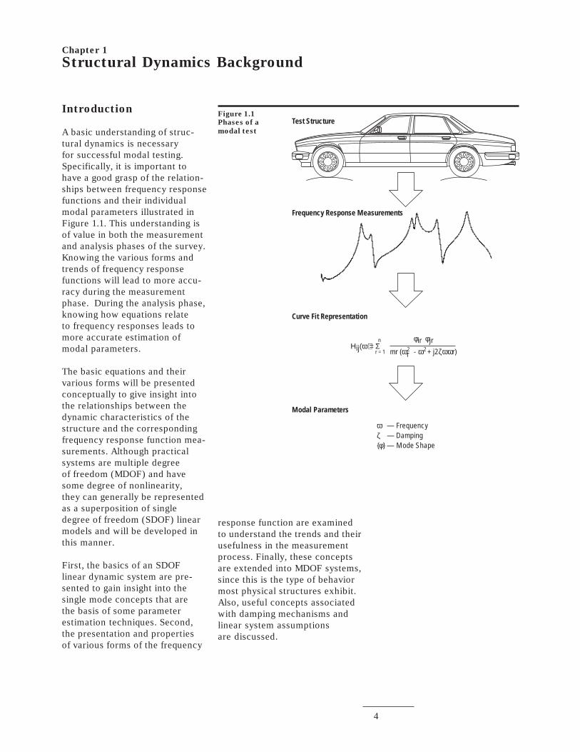
response function are examinedto understand the trends and theirusefulness in the measurementprocess. Finally, these conceptsare extended into MDOF systems,since this is the type of behaviormost physical structures exhibit.Also, useful concepts associatedwith damping mechanisms andlinear system assumptionsare discussed.

Introduction

A basic understanding of struc-tural dynamics is necessaryfor successful modal testing.Specifically, it is important tohave a good grasp of the relation-ships between frequency responsefunctions and their individualmodal parameters illustrated inFigure 1.1. This understanding isof value in both the measurementand analysis phases of the survey.Knowing the various forms andtrends of frequency responsefunctions will lead to more accu-racy during the measurementphase. During the analysis phase,knowing how equations relateto frequency responses leads tomore accurate estimation ofmodal parameters.

The basic equations and theirvarious forms will be presentedconceptually to give insight intothe relationships between thedynamic characteristics of thestructure and the correspondingfrequency response function mea-surements. Although practicalsystems are multiple degreeof freedom (MDOF) and havesome degree of nonlinearity,they can generally be representedas a superposition of singledegree of freedom (SDOF) linearmodels and will be developed inthis manner.

First, the basics of an SDOFlinear dynamic system are pre-sented to gain insight into thesingle mode concepts that arethe basis of some parameterestimation techniques. Second,the presentation and propertiesof various forms of the frequency

Chapter 1

Structural Dynamics Background

Figure 1.1

Phases of a

modal test

Test Structure

Frequency Response Measurements

Modal Parameters

Curve Fit Representation

Η (ω) = Σijn

r = 1

φ φir jrmr ( r - + j2 r)ω ω ζωω2 2

ωζφ

— Frequency— Damping

{ } — Mode Shape

5

Structural Dynamics of aSingle Degree of Freedom(SDOF) System

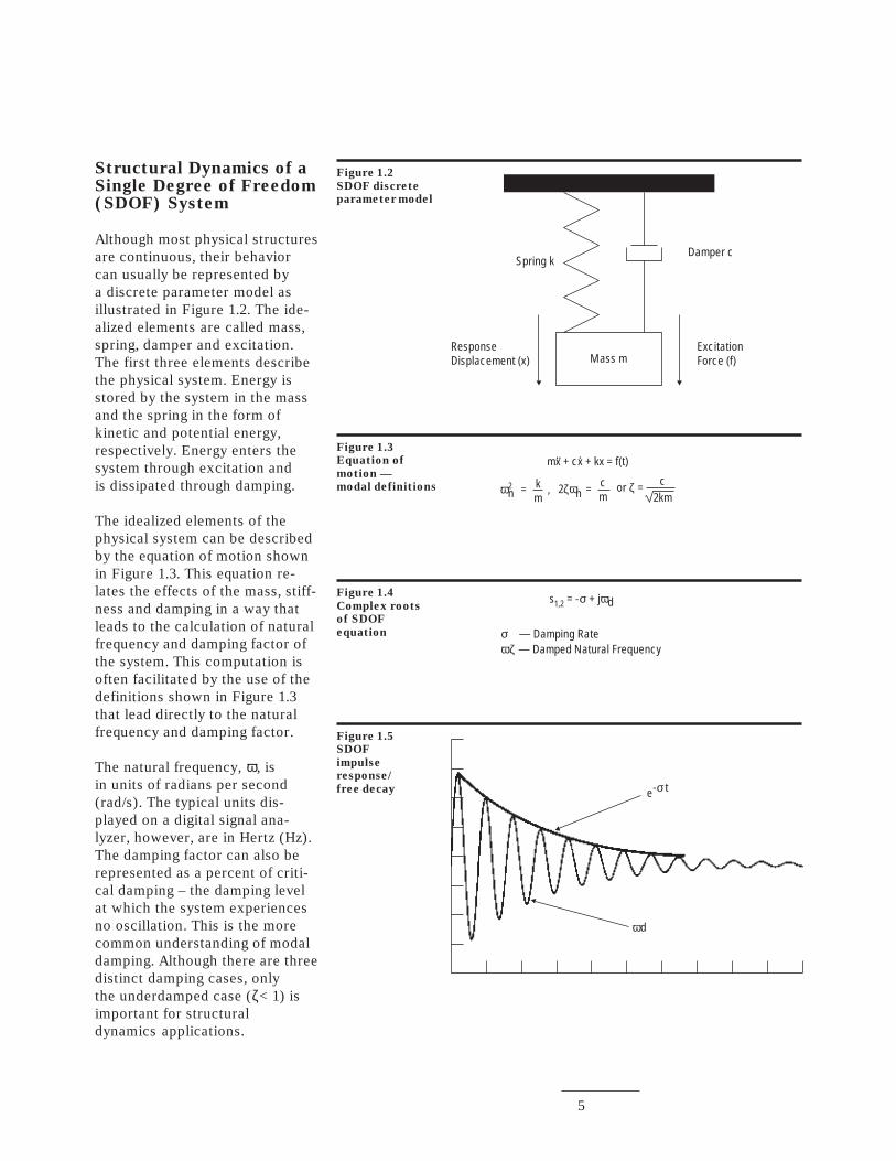
Although most physical structuresare continuous, their behaviorcan usually be represented bya discrete parameter model asillustrated in Figure 1.2. The ide-alized elements are called mass,spring, damper and excitation.The first three elements describethe physical system. Energy isstored by the system in the massand the spring in the form ofkinetic and potential energy,respectively. Energy enters thesystem through excitation andis dissipated through damping.

The idealized elements of thephysical system can be describedby the equation of motion shownin Figure 1.3. This equation re-lates the effects of the mass, stiff-ness and damping in a way thatleads to the calculation of naturalfrequency and damping factor ofthe system. This computation isoften facilitated by the use of thedefinitions shown in Figure 1.3that lead directly to the naturalfrequency and damping factor.

The natural frequency, ω, isin units of radians per second(rad/s). The typical units dis-played on a digital signal ana-lyzer, however, are in Hertz (Hz).The damping factor can also berepresented as a percent of criti-cal damping – the damping levelat which the system experiencesno oscillation. This is the morecommon understanding of modaldamping. Although there are threedistinct damping cases, onlythe underdamped case (ζ< 1) isimportant for structuraldynamics applications.

Figure 1.2

SDOF discrete

parameter model

Spring k

ResponseDisplacement (x) Mass m

Damper c

ExcitationForce (f)

Figure 1.3

Equation of

motion —

modal definitions

Figure 1.4

Complex roots

of SDOF

equation

s = - + j d1,2 σ ω

σωζ

— Damping Rate— Damped Natural Frequency

mx + cx + kx = f(t).. .

ω2n = ,k

m2 n =ζω c

mor =ζ c

2km

Figure 1.5

SDOF

impulse

response/

free decay e- tσ

ωd

6

When there is no excitation,the roots of the equation areas shown in Figure 1.4. Eachroot has two parts: the real partor decay rate, which definesdamping in the system and theimaginary part, or oscillatoryrate, which defines the dampednatural frequency, ωd. This freevibration response is illustratedin Figure 1.5.

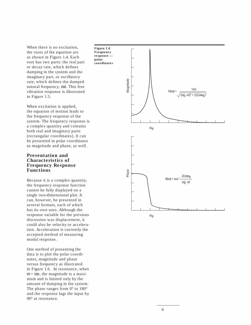
When excitation is applied,the equation of motion leads tothe frequency response of thesystem. The frequency response isa complex quantity and containsboth real and imaginary parts(rectangular coordinates). It canbe presented in polar coordinatesas magnitude and phase, as well.

Presentation andCharacteristics ofFrequency ResponseFunctions

Because it is a complex quantity,the frequency response functioncannot be fully displayed on asingle two-dimensional plot. Itcan, however, be presented inseveral formats, each of whichhas its own uses. Although theresponse variable for the previousdiscussion was displacement, itcould also be velocity or accelera-tion. Acceleration is currently theaccepted method of measuringmodal response.

One method of presenting thedata is to plot the polar coordi-nates, magnitude and phaseversus frequency as illustratedin Figure 1.6. At resonance, whenω = ωn, the magnitude is a maxi-mum and is limited only by theamount of damping in the system.The phase ranges from 0° to 180°and the response lags the input by90° at resonance.

Figure 1.6

Frequency

response —

polar

coordinates

Mag

nitu

dePh

ase

ωd

ωd

H( ) =ω

θ ω( ) = tan-1

1/m

( n- ) + (2 n)ω ω ζωω2 2 2 2

2 n

n-

ξωω

ω ω2 2

7

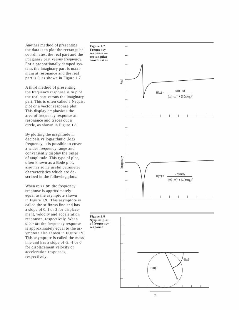
Another method of presentingthe data is to plot the rectangularcoordinates, the real part and theimaginary part versus frequency.For a proportionally damped sys-tem, the imaginary part is maxi-mum at resonance and the realpart is 0, as shown in Figure 1.7.

A third method of presentingthe frequency response is to plotthe real part versus the imaginarypart. This is often called a Nyquistplot or a vector response plot.This display emphasizes thearea of frequency response atresonance and traces out acircle, as shown in Figure 1.8.

By plotting the magnitude indecibels vs logarithmic (log)frequency, it is possible to covera wider frequency range andconveniently display the rangeof amplitude. This type of plot,often known as a Bode plot,also has some useful parametercharacteristics which are de-scribed in the following plots.

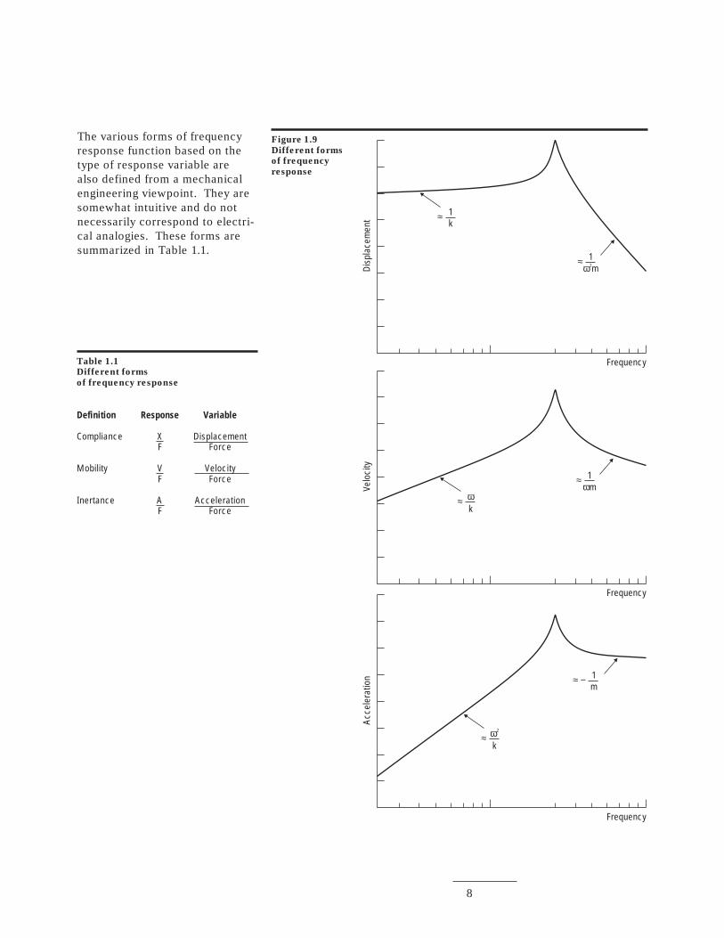
When ω << ωn the frequencyresponse is approximatelyequal to the asymptote shownin Figure 1.9. This asymptote iscalled the stiffness line and hasa slope of 0, 1 or 2 for displace-ment, velocity and accelerationresponses, respectively. Whenω >> ωn the frequency responseis approximately equal to the as-ymptote also shown in Figure 1.9.This asymptote is called the massline and has a slope of -2, -1 or 0for displacement velocity oracceleration responses,respectively.

Figure 1.7

Frequency

response —

rectangular

coordinates

Real

Imag

inar

y

H( ) =ω -2 n

( n- ) + (2 n)

ξωω

ω ω ζωω2 2 2 2

H( ) =ω ω ω

ω ω ζωω

2 2

2 2 2 2

n -

( n- ) + (2 n)

Figure 1.8

Nyquist plot

of frequency

response

θ ω( )

H( )ω

8

The various forms of frequencyresponse function based on thetype of response variable arealso defined from a mechanicalengineering viewpoint. They aresomewhat intuitive and do notnecessarily correspond to electri-cal analogies. These forms aresummarized in Table 1.1.

Figure 1.9

Different forms

of frequency

response

Table 1.1

Different forms

of frequency response

Definition Response Variable

Compliance X DisplacementF Force

Mobility V VelocityF Force

Inertance A AccelerationF Force

Disp

lace

men

tAc

cele

ratio

nVe

loci

tyFrequency

Frequency

Frequency

1k

ω2

k

ωk

1mω2

1m

1mω

≈

≈

≈

≈

≈ −

≈

9

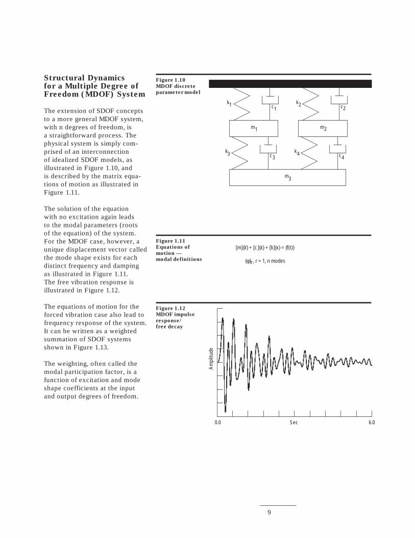
Structural Dynamicsfor a Multiple Degree ofFreedom (MDOF) System

The extension of SDOF conceptsto a more general MDOF system,with n degrees of freedom, isa straightforward process. Thephysical system is simply com-prised of an interconnectionof idealized SDOF models, asillustrated in Figure 1.10, andis described by the matrix equa-tions of motion as illustrated inFigure 1.11.

The solution of the equationwith no excitation again leadsto the modal parameters (rootsof the equation) of the system.For the MDOF case, however, aunique displacement vector calledthe mode shape exists for eachdistinct frequency and dampingas illustrated in Figure 1.11.The free vibration response isillustrated in Figure 1.12.

The equations of motion for theforced vibration case also lead tofrequency response of the system.It can be written as a weightedsummation of SDOF systemsshown in Figure 1.13.

The weighting, often called themodal participation factor, is afunction of excitation and modeshape coefficients at the inputand output degrees of freedom.

Figure 1.10

MDOF discrete

parameter model

k1

k3

k2

k4

c1

c3

c2

c4

m1 m2

m3

Figure 1.11

Equations of

motion —

modal definitions

Figure 1.12

MDOF impulse

response/

free decay

Ampl

itude

0.0 Sec 6.0

[m]{x} + [c]{x} + [k]{x} = {f(t)}

{ }r , r = 1, n modesφ

.. .

10

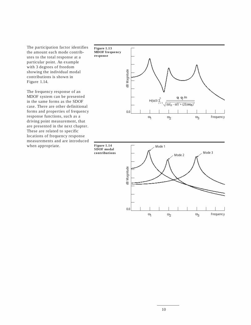
The participation factor identifiesthe amount each mode contrib-utes to the total response at aparticular point. An examplewith 3 degrees of freedomshowing the individual modalcontributions is shown inFigure 1.14.

The frequency response of anMDOF system can be presentedin the same forms as the SDOFcase. There are other definitionalforms and properties of frequencyresponse functions, such as adriving point measurement, thatare presented in the next chapter.These are related to specificlocations of frequency responsemeasurements and are introducedwhen appropriate.

Figure 1.13

MDOF frequency

response

dB M

agni

tude

0.0ω1 ω2 ω3 Frequency

Η(ω) = Σn

r = 1

φ φi j /m

( n - ) + (2 n)ω ω ξωω2 2 2 2

Figure 1.14

SDOF modal

contributions

dB M

agni

tude

0.0ω1 ω2 ω3 Frequency

Mode 1

Mode 2Mode 3

11

measured to characterize the sys-tem when using a linear model.

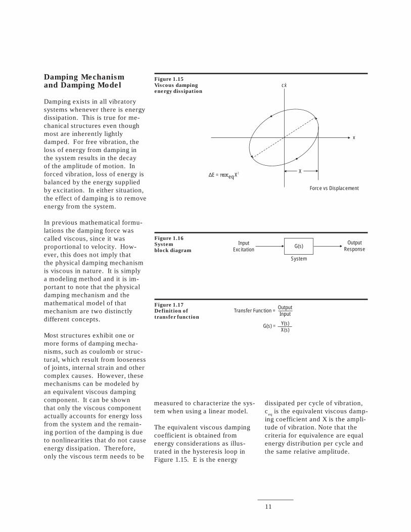
The equivalent viscous dampingcoefficient is obtained fromenergy considerations as illus-trated in the hysteresis loop inFigure 1.15. E is the energy

dissipated per cycle of vibration,c

eq is the equivalent viscous damp-

ing coefficient and X is the ampli-tude of vibration. Note that thecriteria for equivalence are equalenergy distribution per cycle andthe same relative amplitude.

Figure 1.15

Viscous damping

energy dissipation

Damping Mechanismand Damping Model

Damping exists in all vibratorysystems whenever there is energydissipation. This is true for me-chanical structures even thoughmost are inherently lightlydamped. For free vibration, theloss of energy from damping inthe system results in the decayof the amplitude of motion. Inforced vibration, loss of energy isbalanced by the energy suppliedby excitation. In either situation,the effect of damping is to removeenergy from the system.

In previous mathematical formu-lations the damping force wascalled viscous, since it wasproportional to velocity. How-ever, this does not imply thatthe physical damping mechanismis viscous in nature. It is simplya modeling method and it is im-portant to note that the physicaldamping mechanism and themathematical model of thatmechanism are two distinctlydifferent concepts.

Most structures exhibit one ormore forms of damping mecha-nisms, such as coulomb or struc-tural, which result from loosenessof joints, internal strain and othercomplex causes. However, thesemechanisms can be modeled byan equivalent viscous dampingcomponent. It can be shownthat only the viscous componentactually accounts for energy lossfrom the system and the remain-ing portion of the damping is dueto nonlinearities that do not causeenergy dissipation. Therefore,only the viscous term needs to be

x

X∆ πωE = ceq X2

Force vs Displacement

cx.

Figure 1.16

System

block diagram

InputExcitation

System

OutputResponseG(s)

Figure 1.17

Definition of

transfer function

Transfer Function =

G(s) =

OutputInput

Y(s)X(s)

12

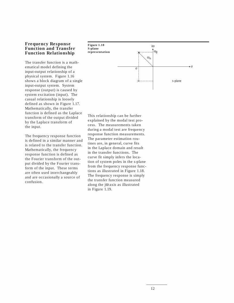
Frequency ResponseFunction and TransferFunction Relationship

The transfer function is a math-ematical model defining theinput-output relationship of aphysical system. Figure 1.16shows a block diagram of a singleinput-output system. Systemresponse (output) is caused bysystem excitation (input). Thecasual relationship is looselydefined as shown in Figure 1.17.Mathematically, the transferfunction is defined as the Laplacetransform of the output dividedby the Laplace transform ofthe input.

The frequency response functionis defined in a similar manner andis related to the transfer function.Mathematically, the frequencyresponse function is defined asthe Fourier transform of the out-put divided by the Fourier trans-form of the input. These termsare often used interchangeablyand are occasionally a source ofconfusion.

Figure 1.18

S-plane

representation

iω

ωn

s-plane

ωd

σσ

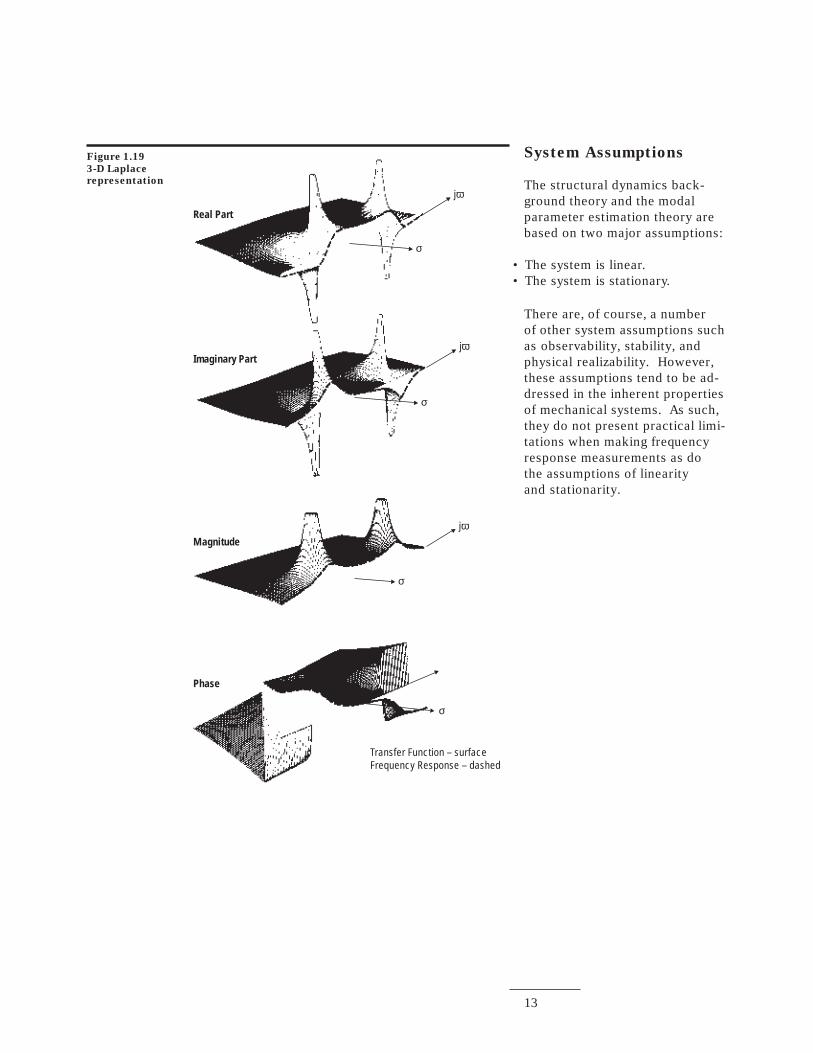
This relationship can be furtherexplained by the modal test pro-cess. The measurements takenduring a modal test are frequencyresponse function measurements.The parameter estimation rou-tines are, in general, curve fitsin the Laplace domain and resultin the transfer functions. Thecurve fit simply infers the loca-tion of system poles in the s-planefrom the frequency response func-tions as illustrated in Figure 1.18.The frequency response is simplythe transfer function measuredalong the jω axis as illustratedin Figure 1.19.

13

System Assumptions

The structural dynamics back-ground theory and the modalparameter estimation theory arebased on two major assumptions:

Figure 1.19

3-D Laplace

representation

• The system is linear.• The system is stationary.

There are, of course, a numberof other system assumptions suchas observability, stability, andphysical realizability. However,these assumptions tend to be ad-dressed in the inherent propertiesof mechanical systems. As such,they do not present practical limi-tations when making frequencyresponse measurements as dothe assumptions of linearityand stationarity.

Real Part

Imaginary Part

Magnitude

Phase

σ

σ

σ

σ

jω

jω

jω

Transfer Function – surfaceFrequency Response – dashed

14

Introduction

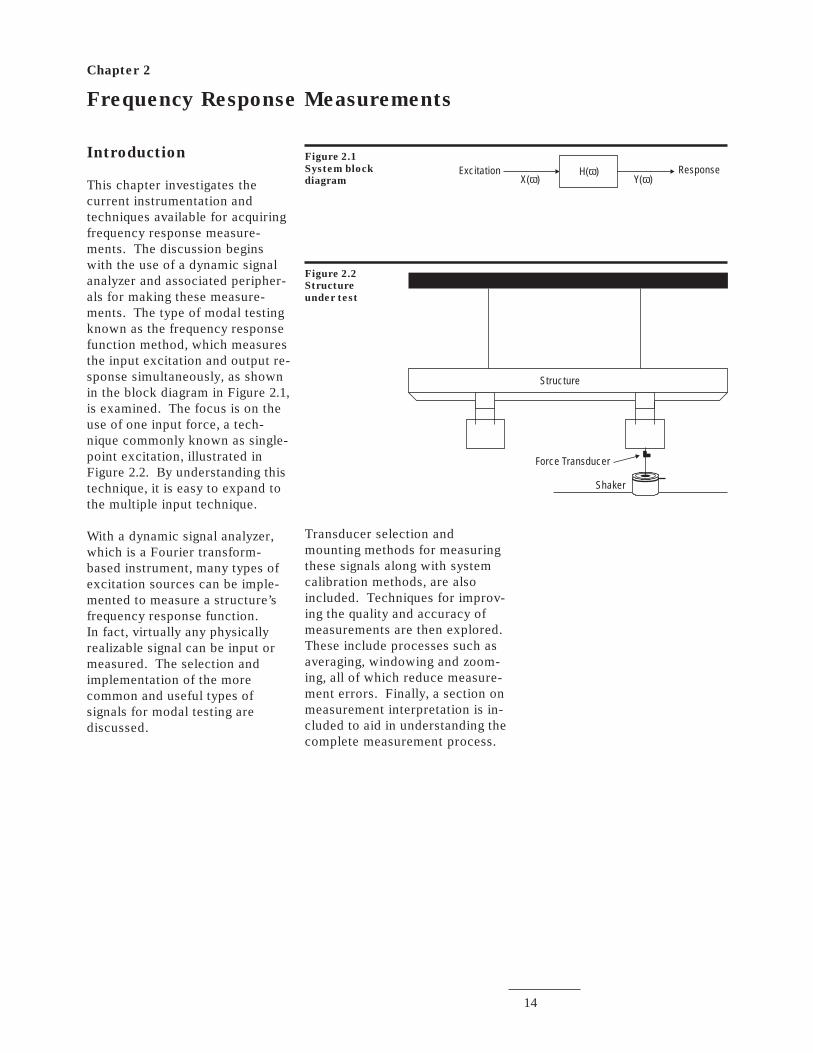
This chapter investigates thecurrent instrumentation andtechniques available for acquiringfrequency response measure-ments. The discussion beginswith the use of a dynamic signalanalyzer and associated peripher-als for making these measure-ments. The type of modal testingknown as the frequency responsefunction method, which measuresthe input excitation and output re-sponse simultaneously, as shownin the block diagram in Figure 2.1,is examined. The focus is on theuse of one input force, a tech-nique commonly known as single-point excitation, illustrated inFigure 2.2. By understanding thistechnique, it is easy to expand tothe multiple input technique.

With a dynamic signal analyzer,which is a Fourier transform-based instrument, many types ofexcitation sources can be imple-mented to measure a structure’sfrequency response function.In fact, virtually any physicallyrealizable signal can be input ormeasured. The selection andimplementation of the morecommon and useful types ofsignals for modal testing arediscussed.

Chapter 2

Frequency Response Measurements

Figure 2.1

System block

diagramExcitation ResponseH( )ω

X( )ω Y( )ω

Figure 2.2

Structure

under test

Structure

Force Transducer

Shaker

Transducer selection andmounting methods for measuringthese signals along with systemcalibration methods, are alsoincluded. Techniques for improv-ing the quality and accuracy ofmeasurements are then explored.These include processes such asaveraging, windowing and zoom-ing, all of which reduce measure-ment errors. Finally, a section onmeasurement interpretation is in-cluded to aid in understanding thecomplete measurement process.

15

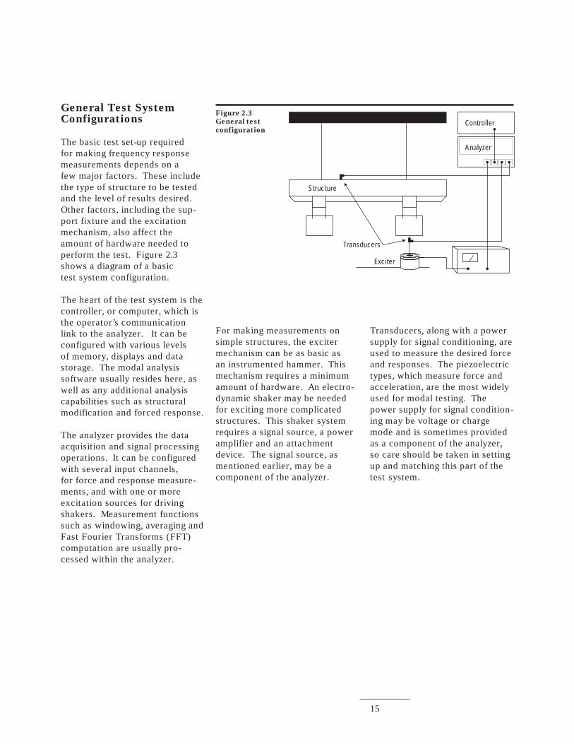
General Test SystemConfigurations

The basic test set-up requiredfor making frequency responsemeasurements depends on afew major factors. These includethe type of structure to be testedand the level of results desired.Other factors, including the sup-port fixture and the excitationmechanism, also affect theamount of hardware needed toperform the test. Figure 2.3shows a diagram of a basictest system configuration.

The heart of the test system is thecontroller, or computer, which isthe operator’s communicationlink to the analyzer. It can beconfigured with various levelsof memory, displays and datastorage. The modal analysissoftware usually resides here, aswell as any additional analysiscapabilities such as structuralmodification and forced response.

The analyzer provides the dataacquisition and signal processingoperations. It can be configuredwith several input channels,for force and response measure-ments, and with one or moreexcitation sources for drivingshakers. Measurement functionssuch as windowing, averaging andFast Fourier Transforms (FFT)computation are usually pro-cessed within the analyzer.

Figure 2.3

General test

configuration

Structure

Transducers

Exciter

Controller

Analyzer

For making measurements onsimple structures, the excitermechanism can be as basic asan instrumented hammer. Thismechanism requires a minimumamount of hardware. An electro-dynamic shaker may be neededfor exciting more complicatedstructures. This shaker systemrequires a signal source, a poweramplifier and an attachmentdevice. The signal source, asmentioned earlier, may be acomponent of the analyzer.

Transducers, along with a powersupply for signal conditioning, areused to measure the desired forceand responses. The piezoelectrictypes, which measure force andacceleration, are the most widelyused for modal testing. Thepower supply for signal condition-ing may be voltage or chargemode and is sometimes providedas a component of the analyzer,so care should be taken in settingup and matching this part of thetest system.

16

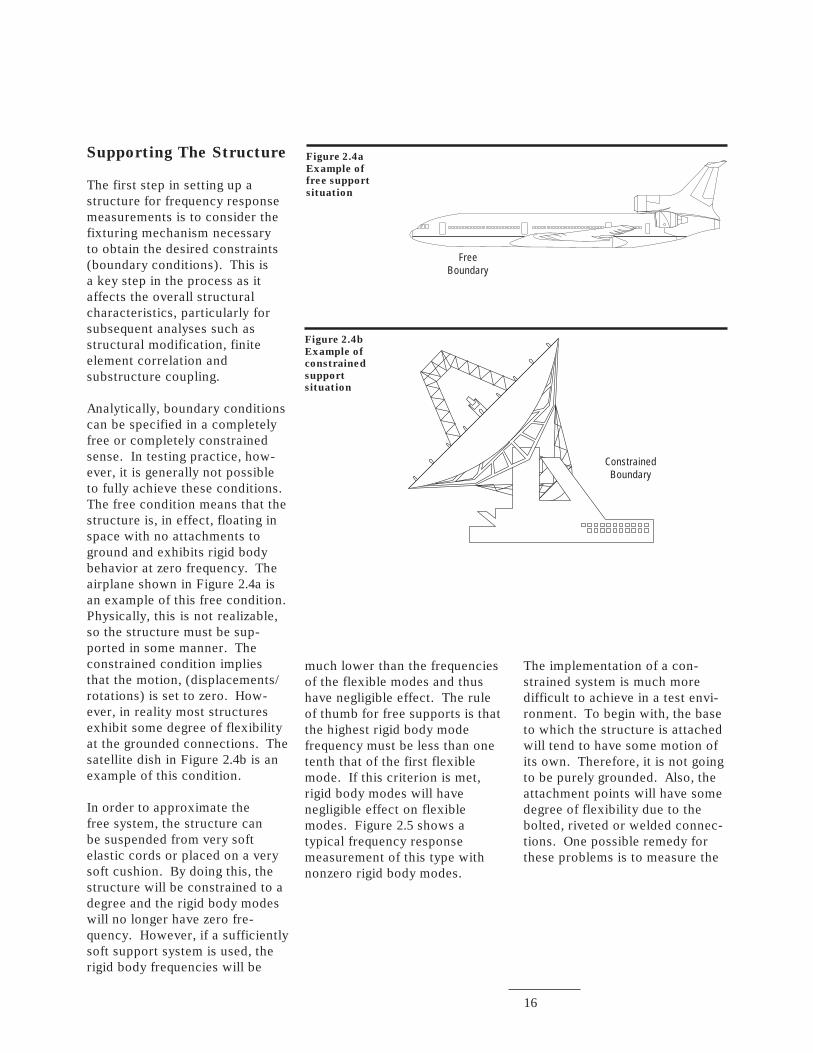
Supporting The Structure

The first step in setting up astructure for frequency responsemeasurements is to consider thefixturing mechanism necessaryto obtain the desired constraints(boundary conditions). This isa key step in the process as itaffects the overall structuralcharacteristics, particularly forsubsequent analyses such asstructural modification, finiteelement correlation andsubstructure coupling.

Analytically, boundary conditionscan be specified in a completelyfree or completely constrainedsense. In testing practice, how-ever, it is generally not possibleto fully achieve these conditions.The free condition means that thestructure is, in effect, floating inspace with no attachments toground and exhibits rigid bodybehavior at zero frequency. Theairplane shown in Figure 2.4a isan example of this free condition.Physically, this is not realizable,so the structure must be sup-ported in some manner. Theconstrained condition impliesthat the motion, (displacements/rotations) is set to zero. How-ever, in reality most structuresexhibit some degree of flexibilityat the grounded connections. Thesatellite dish in Figure 2.4b is anexample of this condition.

In order to approximate thefree system, the structure canbe suspended from very softelastic cords or placed on a verysoft cushion. By doing this, thestructure will be constrained to adegree and the rigid body modeswill no longer have zero fre-quency. However, if a sufficientlysoft support system is used, therigid body frequencies will be

Figure 2.4a

Example of

free support

situation

Figure 2.4b

Example of

constrained

support

situation

ConstrainedBoundary

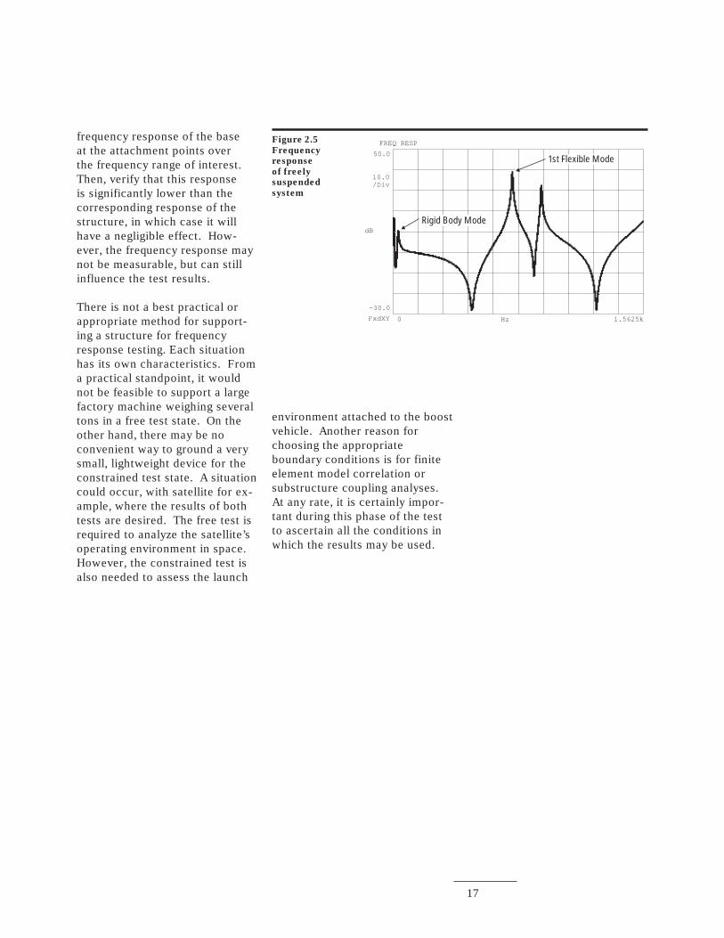
much lower than the frequenciesof the flexible modes and thushave negligible effect. The ruleof thumb for free supports is thatthe highest rigid body modefrequency must be less than onetenth that of the first flexiblemode. If this criterion is met,rigid body modes will havenegligible effect on flexiblemodes. Figure 2.5 shows atypical frequency responsemeasurement of this type withnonzero rigid body modes.

The implementation of a con-strained system is much moredifficult to achieve in a test envi-ronment. To begin with, the baseto which the structure is attachedwill tend to have some motion ofits own. Therefore, it is not goingto be purely grounded. Also, theattachment points will have somedegree of flexibility due to thebolted, riveted or welded connec-tions. One possible remedy forthese problems is to measure the

FreeBoundary

17

frequency response of the baseat the attachment points overthe frequency range of interest.Then, verify that this responseis significantly lower than thecorresponding response of thestructure, in which case it willhave a negligible effect. How-ever, the frequency response maynot be measurable, but can stillinfluence the test results.

There is not a best practical orappropriate method for support-ing a structure for frequencyresponse testing. Each situationhas its own characteristics. Froma practical standpoint, it wouldnot be feasible to support a largefactory machine weighing severaltons in a free test state. On theother hand, there may be noconvenient way to ground a verysmall, lightweight device for theconstrained test state. A situationcould occur, with satellite for ex-ample, where the results of bothtests are desired. The free test isrequired to analyze the satellite’soperating environment in space.However, the constrained test isalso needed to assess the launch

Figure 2.5

Frequency

response

of freely

suspended

system

Hz 1.5625kFxdXY 0

-30.0

dB

10.0/Div

50.0

FREQ RESP

Rigid Body Mode

1st Flexible Mode

environment attached to the boostvehicle. Another reason forchoosing the appropriateboundary conditions is for finiteelement model correlation orsubstructure coupling analyses.At any rate, it is certainly impor-tant during this phase of the testto ascertain all the conditions inwhich the results may be used.

18

Periodic* Transientin analyzer window in analyzer window

Sine True Pseudo Random Fast Impact Burst Burststeady random random sine sine randomstate

Minimze leakage No No Yes Yes Yes Yes Yes Yes

Signal to noise Very Fair Fair Fair High Low High Fairhigh

RMS to peak ratio High Fair Fair Fair High Low High Fair

Test measurement time Very Good Very Fair Fair Very Very Verylong good good good good

Controlled frequency content Yes Yes* Yes* Yes* Yes* No Yes* Yes*

Controlled amplitude content Yes No Yes* No Yes* No Yes* No

Removes distortion No Yes No Yes No No No Yes

Characterize nonlinearity Yes No No No Yes No Yes No

* Requires additional equipment or special hardware

Exciting the Structure

The next step in the measurementprocess involves selecting anexcitation function (e.g., randomnoise) along with an excitationsystem (e.g., a shaker) that bestsuits the application. The choiceof excitation can make the differ-ence between a good measure-ment and a poor one. Excitationselection should be approachedfrom both the type of functiondesired and the type of excitationsystem available because they areinterrelated. The excitation func-tion is the mathematical signalused for the input. The excitationsystem is the physical mechanismused to prove the signal. Gener-ally, the choice of the excitationfunction dictates the choice of theexcitation system, a true randomor burst random function requires

a shaker system for implementa-tion. In general, the reverse isalso true. Choosing a hammerfor the excitation system dictatesan impulsive type excitationfunction.

Excitation functions fall into fourgeneral categories: steady-state,random, periodic and transient.There are several papers thatgo into great detail examining theapplications of the most commonexcitation functions. Table 2.1summarizes the basic characteris-tics of the ones that are mostuseful for modal testing. Truerandom, burst random and im-pulse types are considered in thecontext of this note since they arethe most widely implemented.The best choice of excitationfunction depends on several fac-tors: available signal processing

equipment, characteristics of thestructure, general measurementconsiderations and, of course, theexcitation system.

A full function dynamic signalanalyzer will have a signal sourcewith a sufficient number of func-tions for exciting the structure.With lower quality analyzers,it may be necessary to obtain asignal source as a separate part ofthe signal processing equipment.These sources often provide fixedsine and true random functions assignals; however, these may notbe acceptable in applicationswhere high levels of accuracy aredesired. The types of functionsavailable have a significant influ-ence on measurement quality.

Table 2.1

Excitation

functions

19

The dynamics of the structureare also important in choosing theexcitation function. The level ofnonlinearities can be measuredand characterized effectivelywith sine sweeps or chirps, but arandom function may be neededto estimate the best linearizedmodel of a nonlinear system.The amount of damping and thedensity of the modes within thestructure can also dictate the useof specific excitation functions. Ifmodes are closely coupled and/orlightly damped, an excitationfunction that can be implementedin a leakage-free manner (burstrandom for example) is usuallythe most appropriate.

Excitation mechanisms fall intofour categories: shaker, impactor,step relaxation and self-operating.Step relaxation involvespreloading the structure witha measured force through a

cable then releasing the cableand measuring the transients.Self-operating involves excitingthe structure through an actualoperating load. This input cannotbe measured in many cases, thuslimiting its usefulness. Shakersand impactors are the most com-mon and are discussed in moredetail in the following sections.Another method of excitationmechanism classification is todivide them into attached andnonattached devices. A shakeris an attached device, while animpactor is not, (although it doesmake contact for a short periodof time).

Shaker Testing

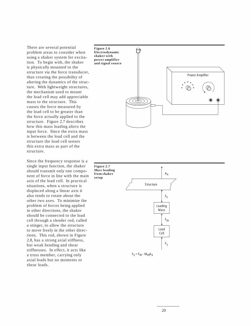
The most useful shakers formodal testing are the electromag-netic shown in Fig. 2.6 (oftencalled electrodynamic) and theelectro hydraulic (or, hydraulic)types. With the electromagneticshaker, (the more common of thetwo), force is generated by analternating current that drives amagnetic coil. The maximum fre-quency limit varies from approxi-mately 5 kHz to 20 kHz dependingon the size; the smaller shakershaving the higher operating range.The maximum force rating isalso a function of the size of theshaker and varies from approxi-mately 2 lbf to 1000 lbf; thesmaller the shaker, the lowerthe force rating.

With hydraulic shakers, forceis generated through the use ofhydraulics, which can providemuch higher force levels – someup to several thousand pounds.The maximum frequency rangeis much lower though – about1 kHz and below. An advantageof the hydraulic shaker is itsability to apply a large staticpreload to the structure. This isuseful for massive structures suchas grinding machines that operateunder relatively high preloadswhich may alter their structuralcharacteristics.

20

There are several potentialproblem areas to consider whenusing a shaker system for excita-tion. To begin with, the shakeris physically mounted to thestructure via the force transducer,thus creating the possibility ofaltering the dynamics of the struc-ture. With lightweight structures,the mechanism used to mountthe load cell may add appreciablemass to the structure. Thiscauses the force measured bythe load cell to be greater thanthe force actually applied to thestructure. Figure 2.7 describeshow this mass loading alters theinput force. Since the extra massis between the load cell and thestructure the load cell sensesthis extra mass as part of thestructure.

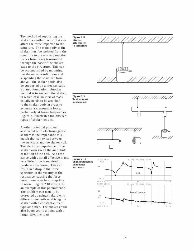
Since the frequency response is asingle input function, the shakershould transmit only one compo-nent of force in line with the mainaxis of the load cell. In practicalsituations, when a structure isdisplaced along a linear axis italso tends to rotate about theother two axes. To minimize theproblem of forces being appliedin other directions, the shakershould be connected to the loadcell through a slender rod, calleda stinger, to allow the structureto move freely in the other direc-tions. This rod, shown in Figure2.8, has a strong axial stiffness,but weak bending and shearstiffnesses. In effect, it acts likea truss member, carrying onlyaxial loads but no moments orshear loads.

Figure 2.6

Electrodynamic

shaker with

power amplifier

and signal source

Power Amplifier

Figure 2.7

Mass loading

from shaker

setup

Ax

Fs

Fm

F1

Fs = Fm - MmAx

LoadingMass

LoadCell

Structure

21

The method of supporting theshaker is another factor that canaffect the force imparted to thestructure. The main body of theshaker must be isolated from thestructure to prevent any reactionforces from being transmittedthrough the base of the shakerback to the structure. This canbe accomplished by mountingthe shaker on a solid floor andsuspending the structure fromabove. The shaker could alsobe supported on a mechanically-isolated foundation. Anothermethod is to suspend the shaker,in which case an inertial massusually needs to be attachedto the shaker body in order togenerate a measurable force,particularly at lower frequencies.Figure 2.9 illustrates the differenttypes of shaker set-ups.

Another potential problemassociated with electromagneticshakers is the impedance mis-match that can exist betweenthe structure and the shaker coil.The electrical impedance of theshaker varies with the amplitudeof motion of the coil. At a reso-nance with a small effective mass,very little force is required toproduce a response. This canresult in a drop in the forcespectrum in the vicinity of theresonance, causing the forcemeasurement to be susceptibleto noise. Figure 2.10 illustratesan example of this phenomenon.The problem can usually becorrected by using shakers withdifferent size coils or driving theshaker with a constant-currenttype amplifier. The shaker couldalso be moved to a point with alarger effective mass.

Figure 2.8

Stinger

attachment

to structure

Figure 2.9

Test support

mechanisms

Figure 2.10

Shaker/structure

impedance

mismatch

POWER SPEC1 30 Avg 50%Ovlp Hann-20.0

dB

-100

Fxd Y 1.1k Hz 2.1k

FREQ RESP 30 Avg 50%Ovlp Hann40.0

dB

-40.0

Fxd Y 1.1k Hz 2.1k

rms

V2

FRF

Force Spectrum

22

Impact Testing

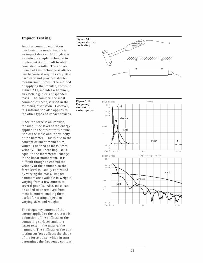
Another common excitationmechanism in modal testing isan impact device. Although it isa relatively simple technique toimplement it’s difficult to obtainconsistent results. The conve-nience of this technique is attrac-tive because it requires very littlehardware and provides shortermeasurement times. The methodof applying the impulse, shown inFigure 2.11, includes a hammer,an electric gun or a suspendedmass. The hammer, the mostcommon of these, is used in thefollowing discussion. However,this information also applies tothe other types of impact devices.

Since the force is an impulse,the amplitude level of the energyapplied to the structure is a func-tion of the mass and the velocityof the hammer. This is due to theconcept of linear momentum,which is defined as mass timesvelocity. The linear impulse isequal to the incremental changein the linear momentum. It isdifficult though to control thevelocity of the hammer, so theforce level is usually controlledby varying the mass. Impacthammers are available in weightsvarying from a few ounces toseveral pounds. Also, mass canbe added to or removed frommost hammers, making themuseful for testing objects ofvarying sizes and weights.

The frequency content of theenergy applied to the structure isa function of the stiffness of thecontacting surfaces and, to alesser extent, the mass of thehammer. The stiffness of the con-tacting surfaces affects the shapeof the force pulse, which in turndetermines the frequency content.

Figure 2.11

Impact devices

for testing

Figure 2.12

Frequency

content of

various pulses

Hz 2.5kFxd X 0

-130

dB

10.0/Div

-50.0

POWER SPEC1 1Avg 0%Ovlp Fr/Ex

rms

v 2

Sec 15.9mFxd Y -46.9µ

-50.0m

Real

50.0m

/Div

350m

FILT TIIME1 0%Ovlp

v

t

Hard

Medium

Soft

Pulse

Soft

Medium

Hard

23

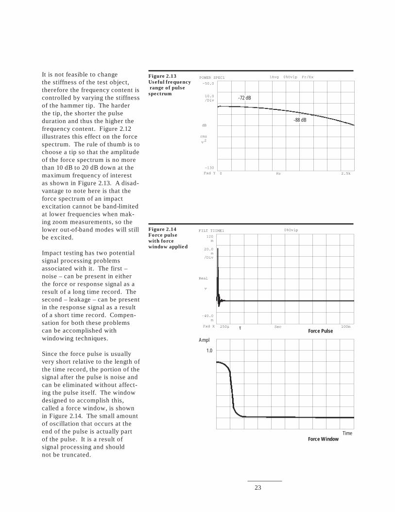
It is not feasible to changethe stiffness of the test object,therefore the frequency content iscontrolled by varying the stiffnessof the hammer tip. The harderthe tip, the shorter the pulseduration and thus the higher thefrequency content. Figure 2.12illustrates this effect on the forcespectrum. The rule of thumb is tochoose a tip so that the amplitudeof the force spectrum is no morethan 10 dB to 20 dB down at themaximum frequency of interestas shown in Figure 2.13. A disad-vantage to note here is that theforce spectrum of an impactexcitation cannot be band-limitedat lower frequencies when mak-ing zoom measurements, so thelower out-of-band modes will stillbe excited.

Impact testing has two potentialsignal processing problemsassociated with it. The first –noise – can be present in eitherthe force or response signal as aresult of a long time record. Thesecond – leakage – can be presentin the response signal as a resultof a short time record. Compen-sation for both these problemscan be accomplished withwindowing techniques.

Since the force pulse is usuallyvery short relative to the length ofthe time record, the portion of thesignal after the pulse is noise andcan be eliminated without affect-ing the pulse itself. The windowdesigned to accomplish this,called a force window, is shownin Figure 2.14. The small amountof oscillation that occurs at theend of the pulse is actually partof the pulse. It is a result ofsignal processing and shouldnot be truncated.

Figure 2.13

Useful frequency

range of pulse

spectrum

Hz 2.5kFxd Y 0

-130

dB

10.0/Div

-50.0

POWER SPEC1 1Avg 0%Ovlp Fr/Ex

rms

v 2

-72 dB

-88 dB

Figure 2.14

Force pulse

with force

window applied

Sec 100mFxd X 250µ

-40.0m

Real

20.0m

/Div

120m

FILT TIIME1 0%Ovlp

v

Force Pulse

TimeForce Window

Ampl

1.0

τ

24

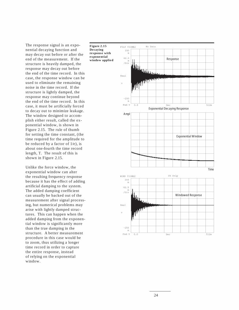
The response signal is an expo-nential decaying function andmay decay out before or after theend of the measurement. If thestructure is heavily damped, theresponse may decay out beforethe end of the time record. In thiscase, the response window can beused to eliminate the remainingnoise in the time record. If thestructure is lightly damped, theresponse may continue beyondthe end of the time record. In thiscase, it must be artificially forcedto decay out to minimize leakage.The window designed to accom-plish either result, called the ex-ponential window, is shown inFigure 2.15. The rule of thumbfor setting the time constant, (thetime required for the amplitude tobe reduced by a factor of 1/e), isabout one-fourth the time recordlength, T. The result of this isshown in Figure 2.15.

Unlike the force window, theexponential window can alterthe resulting frequency responsebecause it has the effect of addingartificial damping to the system.The added damping coefficientcan usually be backed out of themeasurement after signal process-ing, but numerical problems mayarise with lightly damped struc-tures. This can happen when theadded damping from the exponen-tial window is significantly morethan the true damping in thestructure. A better measurementprocedure in this case would beto zoom, thus utilizing a longertime record in order to capturethe entire response, insteadof relying on the exponentialwindow.

Figure 2.15

Decaying

response with

exponential

window applied

Sec

Sec

512m

512m

Fxd Y

Fxd Y

0.0

0.0

-250m

-250m

Real

Real

62.5m

/Div

62.5m

/Div

250m

250m

FILT TIIME2

WIND TIIME2

No Data

0% Ovlp

v

v

Response

Exponential Decaying Response

Exponential Window

Ampl

Time

Windowed Response

25

Transduction

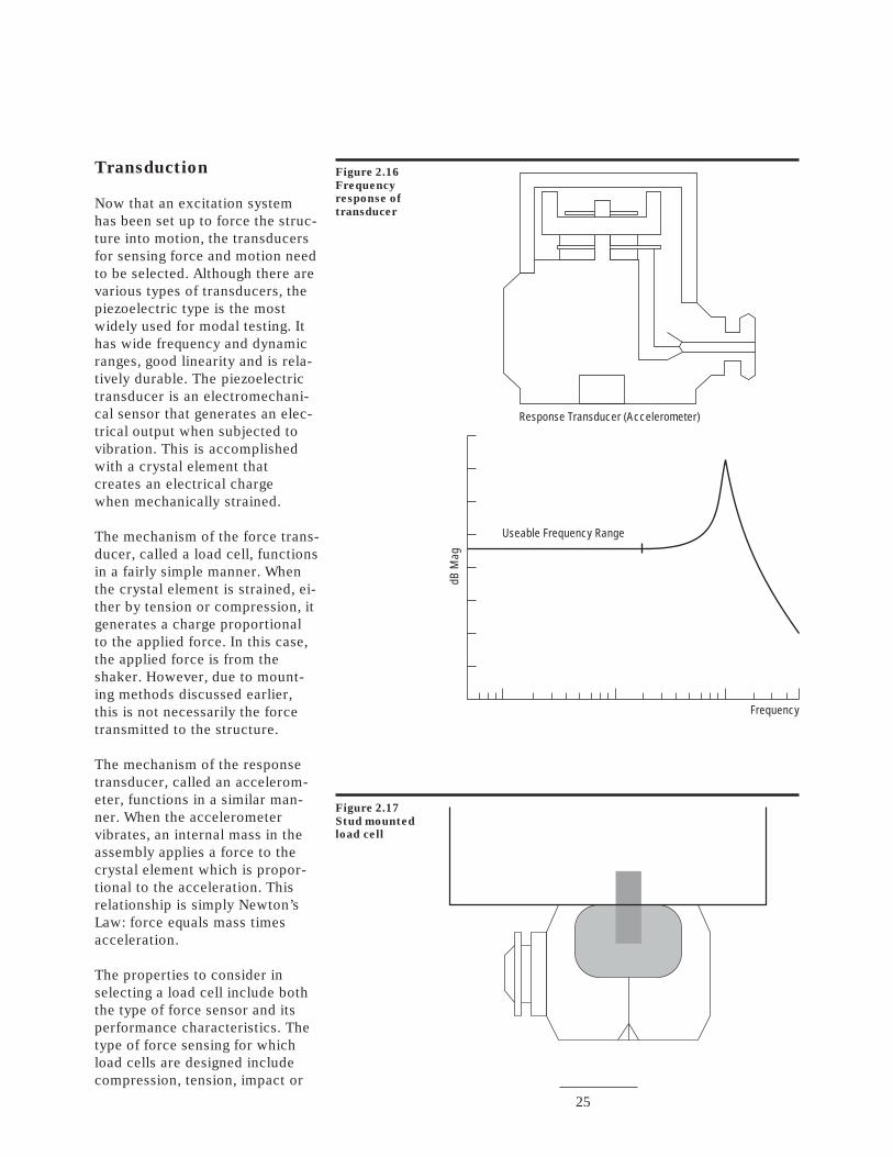
Now that an excitation systemhas been set up to force the struc-ture into motion, the transducersfor sensing force and motion needto be selected. Although there arevarious types of transducers, thepiezoelectric type is the mostwidely used for modal testing. Ithas wide frequency and dynamicranges, good linearity and is rela-tively durable. The piezoelectrictransducer is an electromechani-cal sensor that generates an elec-trical output when subjected tovibration. This is accomplishedwith a crystal element thatcreates an electrical chargewhen mechanically strained.

The mechanism of the force trans-ducer, called a load cell, functionsin a fairly simple manner. Whenthe crystal element is strained, ei-ther by tension or compression, itgenerates a charge proportionalto the applied force. In this case,the applied force is from theshaker. However, due to mount-ing methods discussed earlier,this is not necessarily the forcetransmitted to the structure.

The mechanism of the responsetransducer, called an accelerom-eter, functions in a similar man-ner. When the accelerometervibrates, an internal mass in theassembly applies a force to thecrystal element which is propor-tional to the acceleration. Thisrelationship is simply Newton’sLaw: force equals mass timesacceleration.

The properties to consider inselecting a load cell include boththe type of force sensor and itsperformance characteristics. Thetype of force sensing for whichload cells are designed includecompression, tension, impact or

Figure 2.16

Frequency

response of

transducer

dB M

ag

Frequency

Useable Frequency Range

Response Transducer (Accelerometer)

Figure 2.17

Stud mounted

load cell

26

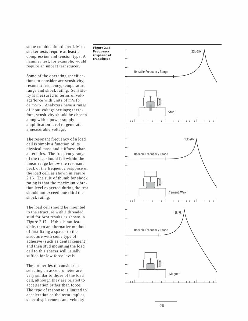
some combination thereof. Mostshaker tests require at least acompression and tension type. Ahammer test, for example, wouldrequire an impact transducer.

Some of the operating specifica-tions to consider are sensitivity,resonant frequency, temperaturerange and shock rating. Sensitiv-ity is measured in terms of volt-age/force with units of mV/1bor mV/N. Analyzers have a rangeof input voltage settings; there-fore, sensitivity should be chosenalong with a power supplyamplification level to generatea measurable voltage.

The resonant frequency of a loadcell is simply a function of itsphysical mass and stiffness char-acteristics. The frequency rangeof the test should fall within thelinear range below the resonantpeak of the frequency response ofthe load cell, as shown in Figure2.16. The rule of thumb for shockrating is that the maximum vibra-tion level expected during the testshould not exceed one third theshock rating.

The load cell should be mountedto the structure with a threadedstud for best results as shown inFigure 2.17. If this is not fea-sible, then an alternative methodof first fixing a spacer to thestructure with some type ofadhesive (such as dental cement)and then stud mounting the loadcell to this spacer will usuallysuffice for low force levels.

The properties to consider inselecting an accelerometer arevery similar to those of the loadcell, although they are related toacceleration rather than force.The type of response is limited toacceleration as the term implies,since displacement and velocity

Figure 2.18

Frequency

response of

transducer

Useable Frequency Range

Useable Frequency Range

Useable Frequency Range

Stud

Cement, Wax

Magnet

20k-25k

15k-20k

5k-7k

27

Figure 2.19

Mass loading

from

accelerometer

Hz 2.5kFxd Y 0

-30.0

dB

10.0/Div

50.0

FREQ RESP 3Avg 0%Ovlp FR/Ex

Frequency

Amplitude

transducers are not available inthe piezoelectric type. However,if displacement or velocityresponses are desired, the accel-eration response can be artifi-cially integrated once or twiceto give velocity and displacementresponses, respectively.

In general, the optimum acceler-ometer has high sensitivity, widefrequency range and small mass.Trade-offs are usually made sincehigh sensitivity usually dictates alarger mass for all but the mostexpensive accelerometers. Thesensitivity, measure in mV/G,and the shock rating should beselected in the same manner aswith the load cell.

Although the resonant frequencyof the accelerometer (freelysuspended) is function of itsmass and stiffness characteris-tics, the actual natural frequency(when mounted) is generallydictated by the stiffness of themounting method used. The effectof various mounting methods isshown in Figure 2.18. The ruleof thumb is to set the maximumfrequency of the test at no morethan one-tenth the mounted natu-ral frequency of the accelerom-eter. This is within the linear

range of the mounted frequencyresponse of the accelerometer.

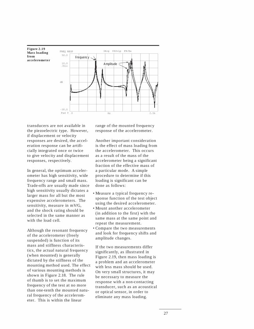
Another important considerationis the effect of mass loading fromthe accelerometer. This occursas a result of the mass of theaccelerometer being a significantfraction of the effective mass ofa particular mode. A simpleprocedure to determine if thisloading is significant can bedone as follows:

If the two measurements differsignificantly, as illustrated inFigure 2.19, then mass loading isa problem and an accelerometerwith less mass should be used.On very small structures, it maybe necessary to measure theresponse with a non-contactingtransducer, such as an acousticalor optical sensor, in order toeliminate any mass loading.

•Measure a typical frequency re-sponse function of the test objectusing the desired accelerometer.

•Mount another accelerometer(in addition to the first) with thesame mass at the same point andrepeat the measurement.

•Compare the two measurementsand look for frequency shifts andamplitude changes.

28

Figure 2.20

Example of

the input

half ranging

Sec 8.0mFxd XY 0.0

-80.0m

Real

20.0m

/Div

80.0m

INST TIME2

FREQ RESP 50 Avg 50% Ovlp Hann40.0

dB

-40.0

Fxd XY 1.1k Hz 2.1k

COHERENCE 50 Avg 50% Ovlp Hann1.1

Mag

0.0

Fxd Y 1.1k Hz 2.1k

v

Figure 2.21

Example of

the input

under ranging

Sec 8.0mFxd XY 0.0

-130m

Real

32.5m

/Div

130m

INST TIME2

FREQ RESP 50 Avg 50% Ovlp Hann40.0

dB

-40.0

Fxd XY 1.1k Hz 2.1k

COHERENCE 50 Avg 50% Ovlp Hann1.1

Mag

0.0

Fxd Y 1.1k Hz 2.1k

v

Figure 2.22

Example of

the input

over ranging

Sec 8.0mFxd X 0.0

-80.0m

Real

20.0m

/Div

80.0m

INST TIME2

FREQ RESP 50 Avg 50% Ovlp Hann40.0

dB

-40.0

Fxd XY 1.1k Hz 2.1k

COHERENCE 50 Avg 50% Ovlp Hann1.1

Mag

0.0

Fxd Y 1.1k Hz 2.1k

v

Ov2

Ov2 Ov2

29

MeasurementInterpretation

Having discussed the mechanicsof setting up a modal test, it isappropriate at this point to makesome trial measurements andexamine their trends beforeproceeding with data collection.Taking the time to investigatepreliminaries of the test, suchas exciter or response locations,various types of excitation func-tions and different signal process-ing parameters will lead to higherquality measurements. This sec-tion includes preliminary checkssuch as adequate signal levels,minimum leakage measurementsand linearity and reciprocitychecks. The concept and trendsof the driving point measurementand the combinations of measure-ments that constitute a completemodal survey are discussed.

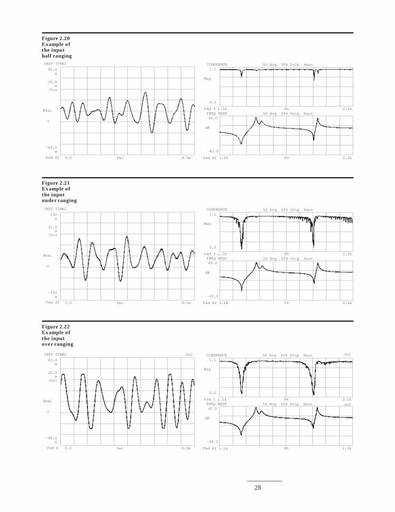
After the structure has beensupported and instrumented forthe test, the time domain signalsshould be examined before mak-ing measurements. The inputrange settings on the analyzershould be set at no more than twotimes the maximum signal levelas shown in Figure 2.20. Oftencalled half-ranging, this takesadvantage of the dynamic rangeof the analog-to-digital converterwithout underranging oroverranging the signals.

The effect resulting from under-ranging a signal, where theresponse input level is severelylow relative to the analyzer set-ting, is illustrated in Figure 2.21.Notice the apparent noise be-tween the peaks in the frequencyresponse and the resultingpoor coherence function. In

Figure 2.23

Random

test signals

Figure 2.24

Transient

test signals

FILT TIME 2 0%Ovlp700

m

Real

-700m

Fxd Y 0.0 Sec 512m

FILT TIME 1 0%Ovlp

400m

Real

-400m

Fxd Y 0.0 Sec 512m

v

v

Typical Force

Exponential Decaying

Response

Figure 2.22, the response isseverely overloading the analyzerinput section and is being clipped.This results in poor frequencyresponse and, consequently,poor coherence since the actualresponse is not being measuredcorrectly.

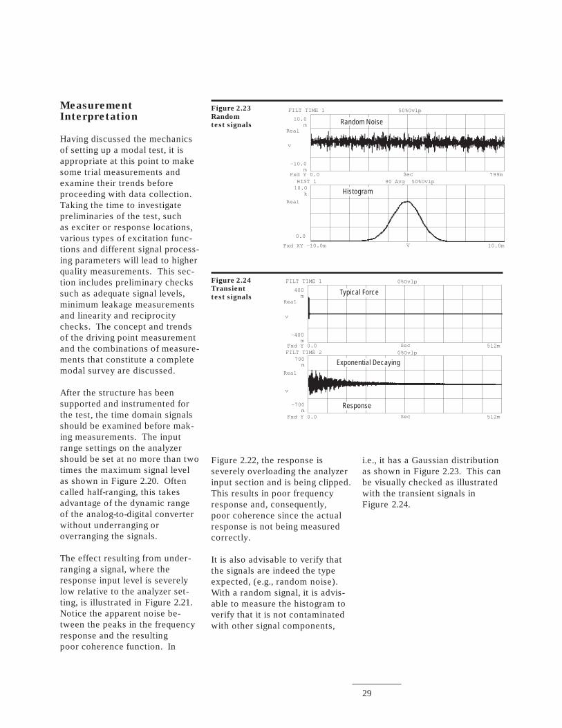
It is also advisable to verify thatthe signals are indeed the typeexpected, (e.g., random noise).With a random signal, it is advis-able to measure the histogram toverify that it is not contaminatedwith other signal components,

i.e., it has a Gaussian distributionas shown in Figure 2.23. This canbe visually checked as illustratedwith the transient signals inFigure 2.24.

HIST 1 90 Avg 50%Ovlp10.0

k

Real

0.0

Fxd XY -10.0m V 10.0m

FILT TIME 1 50%Ovlp

10.0m

Real

-10.0m

Fxd Y 0.0 Sec 799m

v

Histogram

Random Noise

30

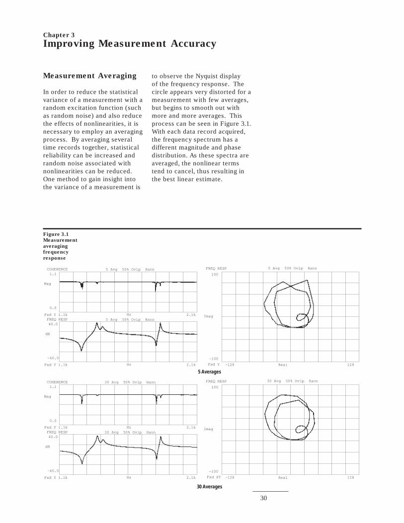
Measurement Averaging

In order to reduce the statisticalvariance of a measurement with arandom excitation function (suchas random noise) and also reducethe effects of nonlinearities, it isnecessary to employ an averagingprocess. By averaging severaltime records together, statisticalreliability can be increased andrandom noise associated withnonlinearities can be reduced.One method to gain insight intothe variance of a measurement is

Chapter 3

Improving Measurement Accuracy

to observe the Nyquist displayof the frequency response. Thecircle appears very distorted for ameasurement with few averages,but begins to smooth out withmore and more averages. Thisprocess can be seen in Figure 3.1.With each data record acquired,the frequency spectrum has adifferent magnitude and phasedistribution. As these spectra areaveraged, the nonlinear termstend to cancel, thus resulting inthe best linear estimate.

Figure 3.1

Measurement

averaging

frequency

response

Real 128Fxd Y -128

-100

Imag

100

FREQ RESP 5 Avg 50% Ovlp Hann

Real 128Fxd XY -128

-100

Imag

100

FREQ RESP 30 Avg 50% Ovlp Hann

FREQ RESP40.0

dB

-40.0

Fxd Y 1.1k Hz 2.1k

COHERENCE 5 Avg 50% Ovlp Hann1.1

Mag

0.0

Fxd Y 1.1k Hz 2.1k5 Avg 50% Ovlp Hann

FREQ RESP40.0

dB

-40.0

Fxd Y 1.1k Hz 2.1k

COHERENCE 30 Avg 50% Ovlp Hann1.1

Mag

0.0

Fxd Y 1.1k Hz 2.1k30 Avg 50% Ovlp Hann

30 Averages

5 Averages

31

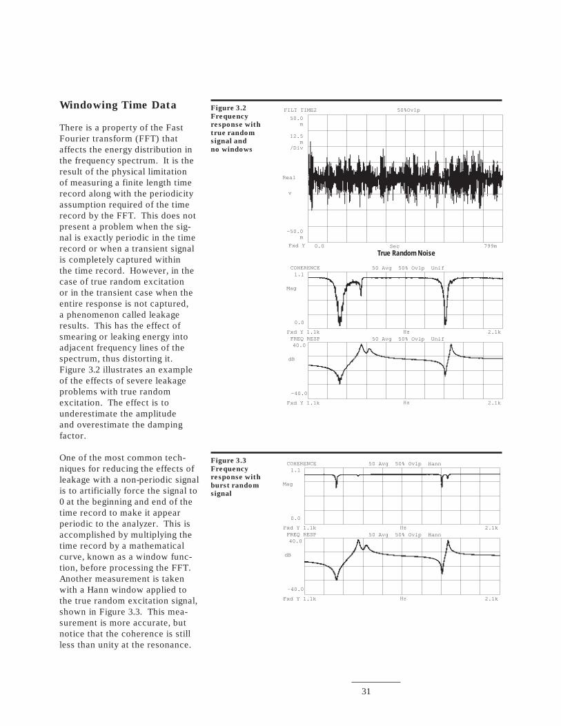
Windowing Time Data

There is a property of the FastFourier transform (FFT) thataffects the energy distribution inthe frequency spectrum. It is theresult of the physical limitationof measuring a finite length timerecord along with the periodicityassumption required of the timerecord by the FFT. This does notpresent a problem when the sig-nal is exactly periodic in the timerecord or when a transient signalis completely captured withinthe time record. However, in thecase of true random excitationor in the transient case when theentire response is not captured,a phenomenon called leakageresults. This has the effect ofsmearing or leaking energy intoadjacent frequency lines of thespectrum, thus distorting it.Figure 3.2 illustrates an exampleof the effects of severe leakageproblems with true randomexcitation. The effect is tounderestimate the amplitudeand overestimate the dampingfactor.

One of the most common tech-niques for reducing the effects ofleakage with a non-periodic signalis to artificially force the signal to0 at the beginning and end of thetime record to make it appearperiodic to the analyzer. This isaccomplished by multiplying thetime record by a mathematicalcurve, known as a window func-tion, before processing the FFT.Another measurement is takenwith a Hann window applied tothe true random excitation signal,shown in Figure 3.3. This mea-surement is more accurate, butnotice that the coherence is stillless than unity at the resonance.

Figure 3.2

Frequency

response with

true random

signal and

no windows

Figure 3.3

Frequency

response with

burst random

signal

Sec 799mFxd Y 0.0

-50.0m

Real

12.5m

/Div

50.0m

FILT TIME2

FREQ RESP 50 Avg 50% Ovlp Unif40.0

dB

-40.0

Fxd Y 1.1k Hz 2.1k

COHERENCE 50 Avg 50% Ovlp Unif1.1

Mag

0.0

Fxd Y 1.1k Hz 2.1k

v

True Random Noise

50%Ovlp

FREQ RESP 50 Avg 50% Ovlp Hann40.0

dB

-40.0

Fxd Y 1.1k Hz 2.1k

COHERENCE 50 Avg 50% Ovlp Hann1.1

Mag

0.0

Fxd Y 1.1k Hz 2.1k

32

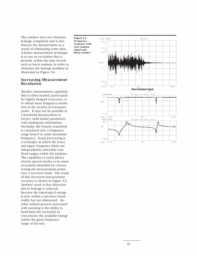
The window does not eliminateleakage completely and it alsodistorts the measurement as aresult of eliminating some data.A better measurement techniqueis to use an excitation that isperiodic within the time recordsuch as burst random, in order toeliminate the leakage problem asillustrated in Figure 3.4.

Increasing MeasurementResolution

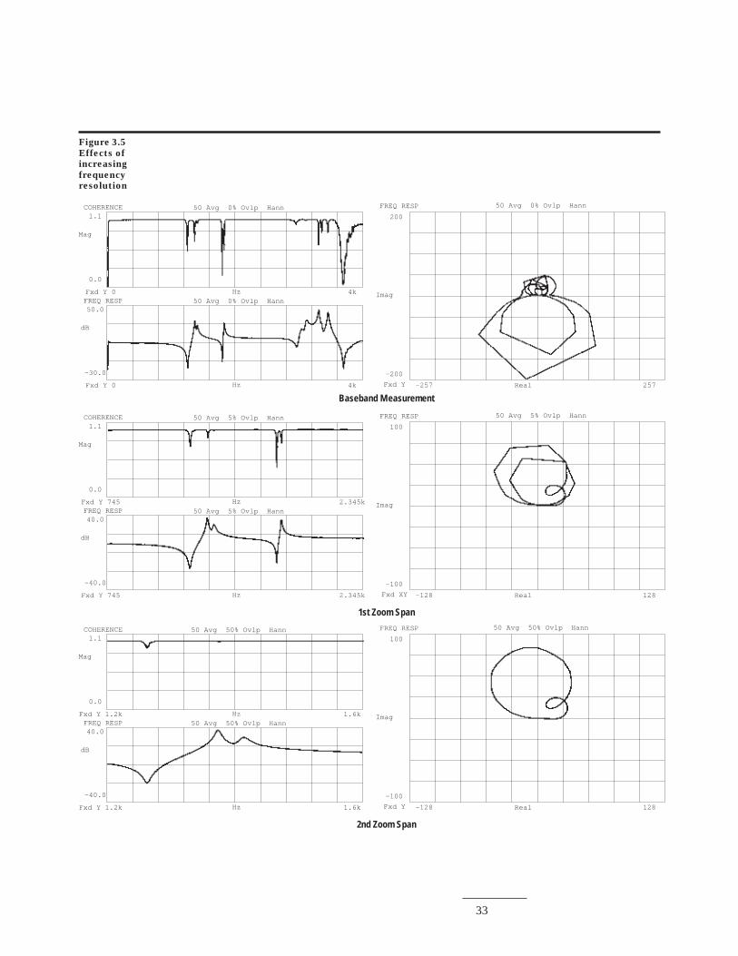
Another measurement capabilitythat is often needed, particularlyfor lightly damped structures, isto obtain more frequency resolu-tion in the vicinity of resonancepeaks. It may not be possible ina baseband measurement toextract valid modal parameterswith inadequate information.Normally, the Fourier transformis calculated over a frequencyrange from 0 to some maximumfrequency. Zoom processing isa technique in which the lowerand upper frequency limits areindependently selectable overfixed ranges within the analyzer.The capability to zoom allowsclosely spaced modes to be moreaccurately identified by concen-trating the measurement pointsover a narrower band. The resultof this increased measurementaccuracy is shown in Figure 3.5.Another result is that distortiondue to leakage is reduced,because the smearing of energyis now within a narrower band-width, but not eliminated. An-other related process associatedwith zooming is the ability toband-limit the excitation toconcentrate the available energywithin the given frequencyrange of the test.

Figure 3.4

Frequency

response with

true random

signal and

Hann window

Sec 799mFxd Y 0.0

-50.0m

Real

12.5m

/Div

50.0m

FILT TIME2

FREQ RESP 15 Avg 0% Ovlp Unif40.0

dB

-40.0

Fxd Y 1.1k Hz 2.1k

COHERENCE 15 Avg 0% Ovlp Unif1.1

Mag

0.0

Fxd Y 1.1k Hz 2.1k

v

Burst Random Signal

0%Ovlp

33

Figure 3.5

Effects of

increasing

frequency

resolution

Real 257Fxd Y -257

-200

Imag

200

FREQ RESP 50 Avg 0% Ovlp Hann

Real

Real

128

128

Fxd XY

Fxd Y

-128

-128

-100

-100

Imag

Imag

100

100

FREQ RESP

FREQ RESP

50 Avg 5% Ovlp Hann

50 Avg 50% Ovlp Hann

FREQ RESP50.0

dB

-30.0

Fxd Y 0 Hz 4k

COHERENCE 50 Avg 0% Ovlp Hann1.1

Mag

0.0

Fxd Y 0 Hz 4k50 Avg 0% Ovlp Hann

FREQ RESP

FREQ RESP

40.0

40.0

dB

dB

-40.0

-40.0

Fxd Y 745

Fxd Y 1.2k

Hz

Hz

2.345k

1.6k

COHERENCE

COHERENCE

50 Avg 5% Ovlp Hann

50 Avg 50% Ovlp Hann

1.1

1.1

Mag

Mag

0.0

0.0

Fxd Y 745

Fxd Y 1.2k

Hz

Hz

2.345k

1.6k

50 Avg 5% Ovlp Hann

50 Avg 50% Ovlp Hann

1st Zoom Span

2nd Zoom Span

Baseband Measurement

34

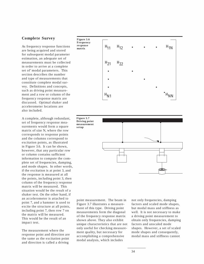
Complete Survey

As frequency response functionsare being acquired and storedfor subsequent modal parameterestimation, an adequate set ofmeasurements must be collectedin order to arrive at a completeset of’ modal parameters. Thissection describes the numberand type of measurements thatconstitute complete modal sur-vey. Definitions and concepts,such as driving point measure-ment and a row or column of thefrequency response matrix arediscussed. Optimal shaker andaccelerometer locations arealso included.

A complete, although redundant,set of frequency response mea-surements would form a squarematrix of size N, where the rowcorresponds to response pointsand the columns correspond toexcitation points, as illustratedin Figure 3.6. It can be shown,however, that any particular rowor column contains sufficientinformation to compute the com-plete set of frequencies, damping,and mode shapes. In other words,if the excitation is at point 3, andthe response is measured at allthe points, including point 3, thencolumn of the frequency responsematrix will be measured. Thissituation would be the result of ashaker test. On the other hand, ifan accelerometer is attached topoint 7, and a hammer is used toexcite the structure at all points,including point 7, then row 7 onthe matrix will be measured.This would be the result of animpact test.

The measurement where theresponse point and direction arethe same as the excitation pointand direction is called a driving

Figure 3.6

Frequency

response

matrix

point measurement. The beam inFigure 3.7 illustrates a measure-ment of this type. Driving pointmeasurements form the diagonalof the frequency response matrixshown above. They also exhibitunique characteristics that are notonly useful for checking measure-ment quality, but necessary foraccomplishing a comprehensivemodal analysis, which includes

not only frequencies, dampingfactors and scaled mode shapes,but modal mass and stiffness aswell. It is not necessary to makea driving point measurement toobtain only frequencies, dampingfactors and unscaled modeshapes. However, a set of scaledmode shapes and consequently,modal mass and stiffness cannot

H11 H12 H1N

H21 H22

HN1 HNN

Figure 3.7

Driving point

measurement

setup

35

be extracted from a set ofmeasurements that does notcontain a driving point.

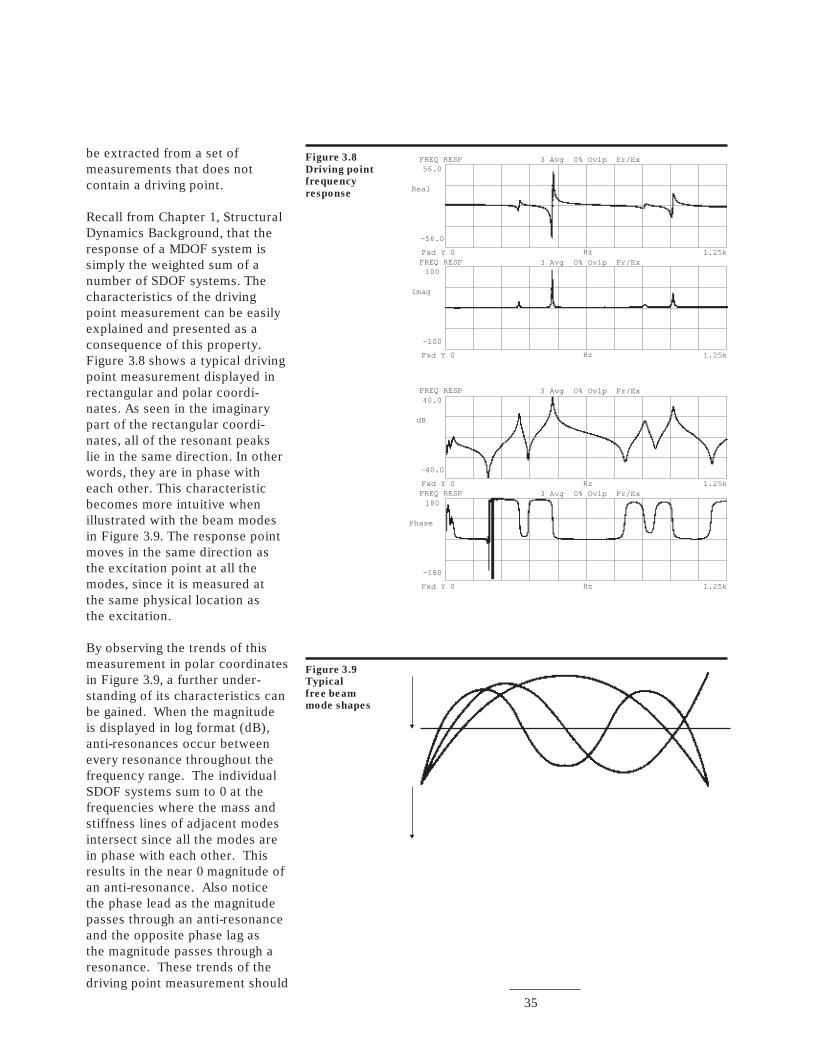
Recall from Chapter 1, StructuralDynamics Background, that theresponse of a MDOF system issimply the weighted sum of anumber of SDOF systems. Thecharacteristics of the drivingpoint measurement can be easilyexplained and presented as aconsequence of this property.Figure 3.8 shows a typical drivingpoint measurement displayed inrectangular and polar coordi-nates. As seen in the imaginarypart of the rectangular coordi-nates, all of the resonant peakslie in the same direction. In otherwords, they are in phase witheach other. This characteristicbecomes more intuitive whenillustrated with the beam modesin Figure 3.9. The response pointmoves in the same direction asthe excitation point at all themodes, since it is measured atthe same physical location asthe excitation.

By observing the trends of thismeasurement in polar coordinatesin Figure 3.9, a further under-standing of its characteristics canbe gained. When the magnitudeis displayed in log format (dB),anti-resonances occur betweenevery resonance throughout thefrequency range. The individualSDOF systems sum to 0 at thefrequencies where the mass andstiffness lines of adjacent modesintersect since all the modes arein phase with each other. Thisresults in the near 0 magnitude ofan anti-resonance. Also noticethe phase lead as the magnitudepasses through an anti-resonanceand the opposite phase lag asthe magnitude passes through aresonance. These trends of thedriving point measurement should

Figure 3.8

Driving point

frequency

response

FREQ RESP100

Imag

-100

Fxd Y 0 Hz 1.25k

FREQ RESP 3 Avg 0% Ovlp Fr/Ex56.0

Real

-56.0

Fxd Y 0 Hz 1.25k3 Avg 0% Ovlp Fr/Ex

FREQ RESP180

Phase

-180

Fxd Y 0 Hz 1.25k

FREQ RESP 3 Avg 0% Ovlp Fr/Ex40.0

dB

-40.0

Fxd Y 0 Hz 1.25k3 Avg 0% Ovlp Fr/Ex

Figure 3.9

Typical

free beam

mode shapes

36

be observed and monitoredthroughout the measurementprocess as a check for maintain-ing a consistent set of data.

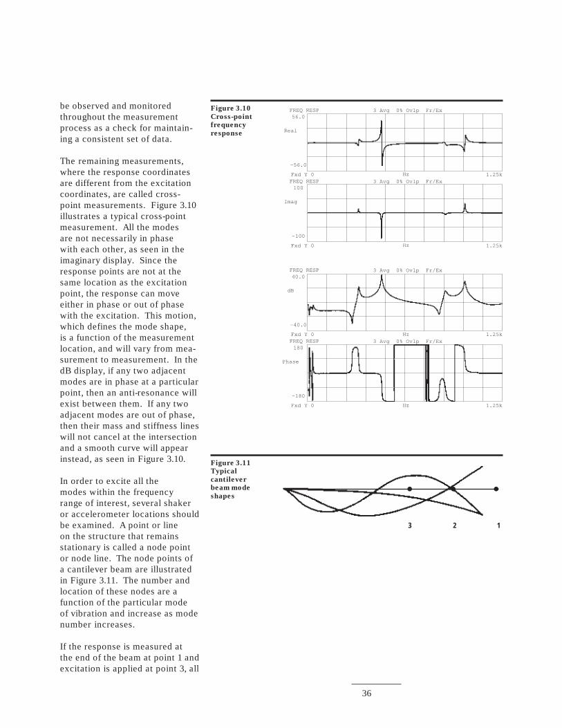
The remaining measurements,where the response coordinatesare different from the excitationcoordinates, are called cross-point measurements. Figure 3.10illustrates a typical cross-pointmeasurement. All the modesare not necessarily in phasewith each other, as seen in theimaginary display. Since theresponse points are not at thesame location as the excitationpoint, the response can moveeither in phase or out of phasewith the excitation. This motion,which defines the mode shape,is a function of the measurementlocation, and will vary from mea-surement to measurement. In thedB display, if any two adjacentmodes are in phase at a particularpoint, then an anti-resonance willexist between them. If any twoadjacent modes are out of phase,then their mass and stiffness lineswill not cancel at the intersectionand a smooth curve will appearinstead, as seen in Figure 3.10.

In order to excite all themodes within the frequencyrange of interest, several shakeror accelerometer locations shouldbe examined. A point or lineon the structure that remainsstationary is called a node pointor node line. The node points ofa cantilever beam are illustratedin Figure 3.11. The number andlocation of these nodes are afunction of the particular modeof vibration and increase as modenumber increases.

If the response is measured atthe end of the beam at point 1 andexcitation is applied at point 3, all

Figure 3.10

Cross-point

frequency

response

FREQ RESP100

Imag

-100

Fxd Y 0 Hz 1.25k

FREQ RESP 3 Avg 0% Ovlp Fr/Ex56.0

Real

-56.0

Fxd Y 0 Hz 1.25k3 Avg 0% Ovlp Fr/Ex

FREQ RESP180

Phase

-180

Fxd Y 0 Hz 1.25k

FREQ RESP 3 Avg 0% Ovlp Fr/Ex40.0

dB

-40.0

Fxd Y 0 Hz 1.25k3 Avg 0% Ovlp Fr/Ex

Figure 3.11

Typical

cantilever

beam mode

shapes

2 13

37

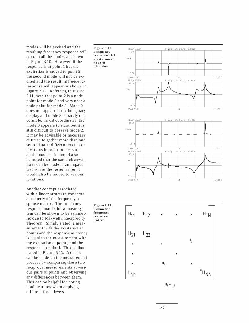
modes will be excited and theresulting frequency response willcontain all the modes as shownin Figure 3.10. However, if theresponse is at point 1 but theexcitation is moved to point 2,the second mode will not be ex-cited and the resulting frequencyresponse will appear as shown inFigure 3.12. Referring to Figure3.11, note that point 2 is a nodepoint for mode 2 and very near anode point for mode 3. Mode 2does not appear in the imaginarydisplay and mode 3 is barely dis-cernible. In dB coordinates, themode 3 appears to exist but it isstill difficult to observe mode 2.It may be advisable or necessaryat times to gather more than oneset of data at different excitationlocations in order to measureall the modes. It should alsobe noted that the same observa-tions can be made in an impacttest where the response pointwould also be moved to variouslocations.

Another concept associatedwith a linear structure concernsa property of the frequency re-sponse matrix. The frequencyresponse matrix for a linear sys-tem can be shown to be symmet-ric due to Maxwell’s ReciprocityTheorem. Simply stated, a mea-surement with the excitation atpoint i and the response at point jis equal to the measurement withthe excitation at point j and theresponse at point i. This is illus-trated in Figure 3.13. A checkcan be made on the measurementprocess by comparing these tworeciprocal measurements at vari-ous pairs of points and observingany differences between them.This can be helpful for notingnonlinearities when applyingdifferent force levels.

Figure 3.12

Frequency

response with

excitation at

node of

vibration

FREQ RESP40.0

dB

-40.0

Fxd Y 0 Hz 1.25k

FREQ RESP 3 Avg 0% Ovlp Fr/Ex100

Imag

-100

Fxd Y 0 Hz 1.25k3 Avg 0% Ovlp Fr/Ex

FREQ RESP40.0

dB

-40.0

Fxd Y 0 Hz 1.25k

FREQ RESP 3 Avg 0% Ovlp Fr/Ex56.0

Imag

-56.0

Fxd Y 0 Hz 1.25k3 Avg 0% Ovlp Fr/Ex

Figure 3.13

Symmetric

frequency

response

matrix

H11 H12 H1N

H21 H22

HN1 HNN

Hji

Hij

Hij = Hji

38

Introduction

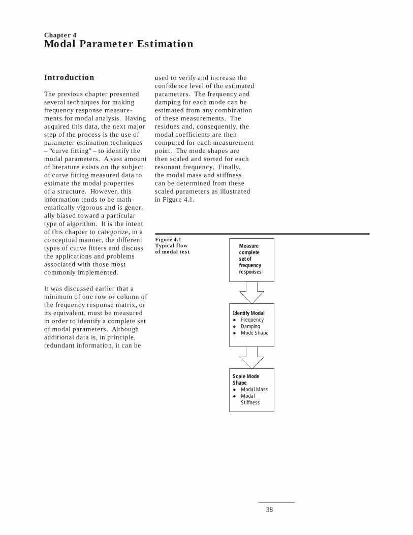
The previous chapter presentedseveral techniques for makingfrequency response measure-ments for modal analysis. Havingacquired this data, the next majorstep of the process is the use ofparameter estimation techniques– “curve fitting” – to identify themodal parameters. A vast amountof literature exists on the subjectof curve fitting measured data toestimate the modal propertiesof a structure. However, thisinformation tends to be math-ematically vigorous and is gener-ally biased toward a particulartype of algorithm. It is the intentof this chapter to categorize, in aconceptual manner, the differenttypes of curve fttters and discussthe applications and problemsassociated with those mostcommonly implemented.

It was discussed earlier that aminimum of one row or column ofthe frequency response matrix, orits equivalent, must be measuredin order to identify a complete setof modal parameters. Althoughadditional data is, in principle,redundant information, it can be

Chapter 4

Modal Parameter Estimation

used to verify and increase theconfidence level of the estimatedparameters. The frequency anddamping for each mode can beestimated from any combinationof these measurements. Theresidues and, consequently, themodal coefficients are thencomputed for each measurementpoint. The mode shapes arethen scaled and sorted for eachresonant frequency. Finally,the modal mass and stiffnesscan be determined from thesescaled parameters as illustratedin Figure 4.1.

Figure 4.1

Typical flow

of modal test

Scale ModeShapel

l

Modal MassModalStiffness

Measurecompleteset offrequencyresponses

Identify Modall

l

l

FrequencyDampingMode Shape

39

Modal Parameters

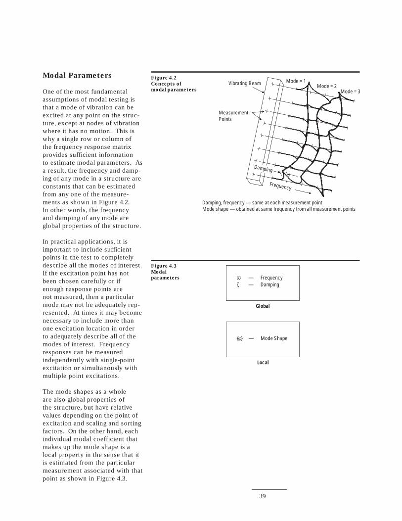
One of the most fundamentalassumptions of modal testing isthat a mode of vibration can beexcited at any point on the struc-ture, except at nodes of vibrationwhere it has no motion. This iswhy a single row or column ofthe frequency response matrixprovides sufficient informationto estimate modal parameters. Asa result, the frequency and damp-ing of any mode in a structure areconstants that can be estimatedfrom any one of the measure-ments as shown in Figure 4.2.In other words, the frequencyand damping of any mode areglobal properties of the structure.

In practical applications, it isimportant to include sufficientpoints in the test to completelydescribe all the modes of interest.If the excitation point has notbeen chosen carefully or ifenough response points arenot measured, then a particularmode may not be adequately rep-resented. At times it may becomenecessary to include more thanone excitation location in orderto adequately describe all of themodes of interest. Frequencyresponses can be measuredindependently with single-pointexcitation or simultanously withmultiple point excitations.

The mode shapes as a wholeare also global properties ofthe structure, but have relativevalues depending on the point ofexcitation and scaling and sortingfactors. On the other hand, eachindividual modal coefficient thatmakes up the mode shape is alocal property in the sense that itis estimated from the particularmeasurement associated with thatpoint as shown in Figure 4.3.

Figure 4.2

Concepts of

modal parameters

Frequency

Damping

Mode = 1Mode = 2

Mode = 3

Vibrating Beam

MeasurementPoints

Damping, frequency — same at each measurement pointMode shape — obtained at same frequency from all measurement points

Figure 4.3

Modal

parameters ωζ

— Frequency— Damping

{ } — Mode Shapeφ

Global

Local

40

Curve Fitting Methods

Due to the large amount ofliterature and algorithmscurrently available for curvefitting structural data, it has be-come difficult to determine theexact need for each method andwhich method is best. There is noideal solution and the commonmethods are only approximations.Also, many of the methods arevery similar to each other and,in some cases, simply extensionsof a few basic techniques.

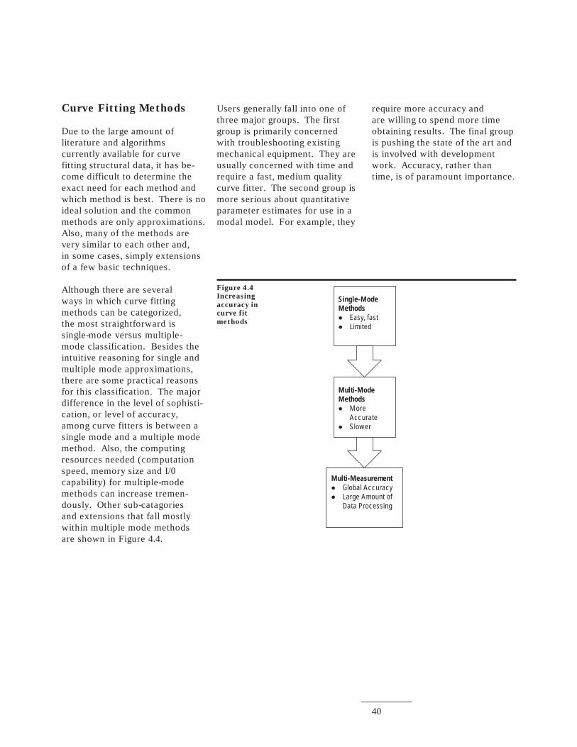
Although there are severalways in which curve fittingmethods can be categorized,the most straightforward issingle-mode versus multiple-mode classification. Besides theintuitive reasoning for single andmultiple mode approximations,there are some practical reasonsfor this classification. The majordifference in the level of sophisti-cation, or level of accuracy,among curve fitters is between asingle mode and a multiple modemethod. Also, the computingresources needed (computationspeed, memory size and I/0capability) for multiple-modemethods can increase tremen-dously. Other sub-catagoriesand extensions that fall mostlywithin multiple mode methodsare shown in Figure 4.4.

Users generally fall into one ofthree major groups. The firstgroup is primarily concernedwith troubleshooting existingmechanical equipment. They areusually concerned with time andrequire a fast, medium qualitycurve fitter. The second group ismore serious about quantitativeparameter estimates for use in amodal model. For example, they

require more accuracy andare willing to spend more timeobtaining results. The final groupis pushing the state of the art andis involved with developmentwork. Accuracy, rather thantime, is of paramount importance.

Figure 4.4

Increasing

accuracy in

curve fit

methods

Multi-Measurementl

l

Global AccuracyLarge Amount ofData Processing

Single-ModeMethodsl

l

Easy, fastLimited

Multi-ModeMethodsl

l

MoreAccurateSlower

41

Single-Mode Methods

As stated earlier, the generalprocedure for estimating modalparameters is to estimate frequen-cies and damping factors, thenestimate modal coefficients.For most single-mode parameterestimation techniques, however,this is not always the case. Infact, it is not absolutely necessaryto estimate damping in order toobtain modal coefficients. Thisis typical in a troubleshootingenvironment where frequenciesand mode shapes are of primaryconcern.

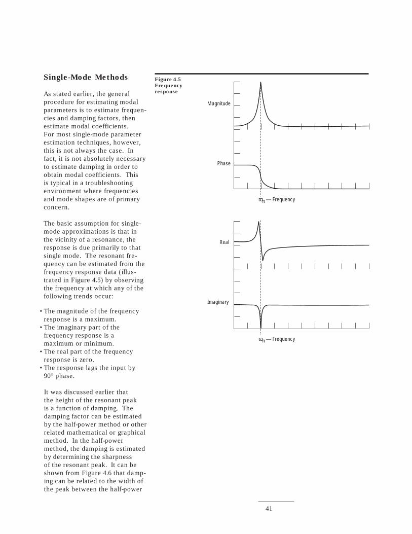
The basic assumption for single-mode approximations is that inthe vicinity of a resonance, theresponse is due primarily to thatsingle mode. The resonant fre-quency can be estimated from thefrequency response data (illus-trated in Figure 4.5) by observingthe frequency at which any of thefollowing trends occur:

Figure 4.5

Frequency

response

ωn — Frequency

Real

Imaginary

ωn — Frequency

Magnitude

Phase

•The magnitude of the frequencyresponse is a maximum.

•The imaginary part of thefrequency response is amaximum or minimum.

•The real part of the frequencyresponse is zero.

•The response lags the input by90° phase.

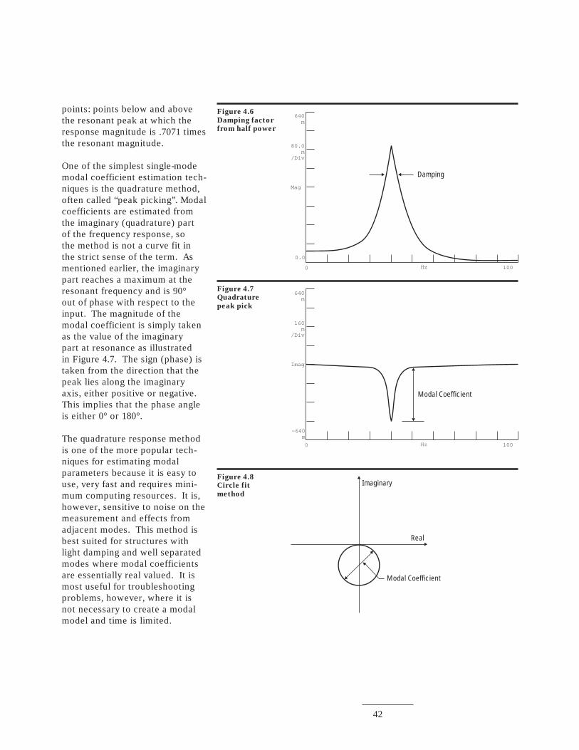
It was discussed earlier thatthe height of the resonant peakis a function of damping. Thedamping factor can be estimatedby the half-power method or otherrelated mathematical or graphicalmethod. In the half-powermethod, the damping is estimatedby determining the sharpnessof the resonant peak. It can beshown from Figure 4.6 that damp-ing can be related to the width ofthe peak between the half-power

42

points: points below and abovethe resonant peak at which theresponse magnitude is .7071 timesthe resonant magnitude.

One of the simplest single-modemodal coefficient estimation tech-niques is the quadrature method,often called “peak picking”. Modalcoefficients are estimated fromthe imaginary (quadrature) partof the frequency response, sothe method is not a curve fit inthe strict sense of the term. Asmentioned earlier, the imaginarypart reaches a maximum at theresonant frequency and is 90°out of phase with respect to theinput. The magnitude of themodal coefficient is simply takenas the value of the imaginarypart at resonance as illustratedin Figure 4.7. The sign (phase) istaken from the direction that thepeak lies along the imaginaryaxis, either positive or negative.This implies that the phase angleis either 0° or 180°.

The quadrature response methodis one of the more popular tech-niques for estimating modalparameters because it is easy touse, very fast and requires mini-mum computing resources. It is,however, sensitive to noise on themeasurement and effects fromadjacent modes. This method isbest suited for structures withlight damping and well separatedmodes where modal coefficientsare essentially real valued. It ismost useful for troubleshootingproblems, however, where it isnot necessary to create a modalmodel and time is limited.

Figure 4.6

Damping factor

from half power

640m

80.0m

/Div

Mag

0.0

0 Hz 100

Damping

Figure 4.7

Quadrature

peak pick

640m

160m

/Div

Imag

-640m

0 Hz 100

Modal Coefficient

Figure 4.8

Circle fit

method

Imaginary

Real

Modal Coefficient

43

Another single-mode technique,called the circle fit, was originallydeveloped for structural dampingbut can be extended to theviscous damping case. Recallfrom Chapter 1 that the frequencyresponse of a mode traces out acircle in the imaginary plane.The method fits a circle to thereal and imaginary part of thefrequency response data byminimizing the error betweenthe radius of the fitted circle andthe measured data. The modalcoefficient is then determinedfrom the diameter of the circleas illustrated in Figure 4.8. Thephase is determined from thepositive or negative half of theimaginary axis in which thecircle lies.

Frequency and damping can beestimated by one of the methodsdiscussed earlier or by some ofthe MDOF methods to be dis-cussed later. Damping can alsobe estimated from the spacingof points along the Nyquist plotfrom the circle.

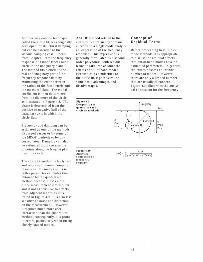
The circle fit method is fairly fastand requires minimum computerresources. It usually results inbetter parameter estimates thanobtained by the quadraturemethod because it uses moreof the measurement informationand is not as sensitive to effectsfrom adjacent modes as illus-trated in Figure 4.9. It is also lesssensitive to noise and distortionon the measurement. However,it requires much more userinteraction than the quadraturemethod; consequently, it is proneto errors, particularly when fittingclosely spaced modes.

A SDOF method related to thecircle fit is a frequency domaincurve fit to a single-mode analyti-cal expression of the frequencyresponse. This expression isgenerally formulated as a secondorder polynomial with residualterms to take into account theeffects of out of band modes.Because of its similarities tothe circle fit, it possesses thesame basic advantages anddisadvantages.

Concept ofResidual Terms

Before proceeding to multiple-mode methods, it is appropriateto discuss the residual effectsthat out-of-band modes have onestimated parameters. In general,structures possess an infinitenumber of modes. However,there are only a limited numberthat are usually of concern.Figure 4.10 illustrates the analyti-cal expression for the frequency

Figure 4.9

Comparison of

quadrature and

circle fit methods

Imaginary

Real

φPeakPick

φPeakPick

φ Circle Fit

φ Circle Fit

Figure 4.10

Analytical

expression of

frequency

response

H( ) =ωn

r = 1Σ

φ φi j( n - ) + j(2 n)ω ω ζωω2 2

44

response of a structure takinginto account the total number ofrealizable modes. Unfortunately,the measured frequency responseis limited to some frequencyrange of interest depending on thecapabilities of the analyzer andthe frequency resolution desired.This range may not necessarilyinclude several lower frequencymodes and most certainly will notinclude some higher frequencymodes. However, the residualeffects of these out-of-bandmodes will be present in themeasurement and, consequently,affect the accuracy of parameterestimation.

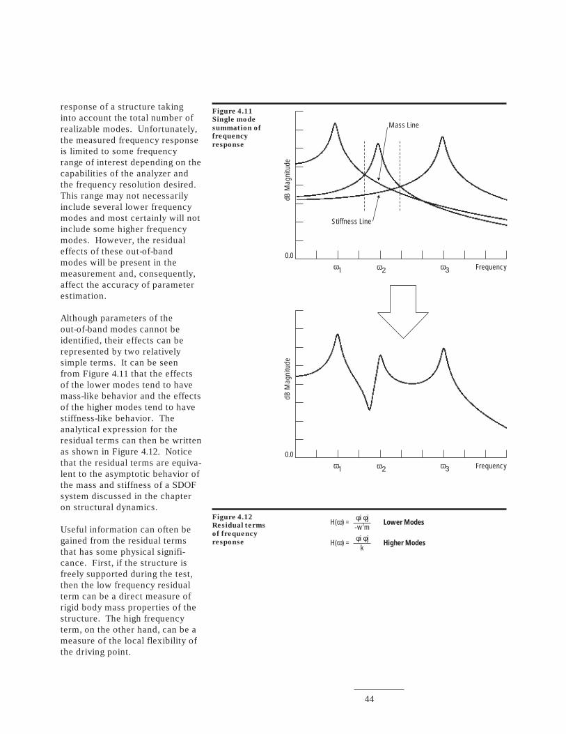
Although parameters of theout-of-band modes cannot beidentified, their effects can berepresented by two relativelysimple terms. It can be seenfrom Figure 4.11 that the effectsof the lower modes tend to havemass-like behavior and the effectsof the higher modes tend to havestiffness-like behavior. Theanalytical expression for theresidual terms can then be writtenas shown in Figure 4.12. Noticethat the residual terms are equiva-lent to the asymptotic behavior ofthe mass and stiffness of a SDOFsystem discussed in the chapteron structural dynamics.

Useful information can often begained from the residual termsthat has some physical signifi-cance. First, if the structure isfreely supported during the test,then the low frequency residualterm can be a direct measure ofrigid body mass properties of thestructure. The high frequencyterm, on the other hand, can be ameasure of the local flexibility ofthe driving point.

Figure 4.11

Single mode

summation of

frequency

response

dB M

agni

tude

0.0ω1 ω2 ω3 Frequency

dB M

agni

tude

0.0ω1 ω2 ω3 Frequency

Mass Line

Stiffness Line

Figure 4.12

Residual terms

of frequency

response H( ) =ω φ φi jk

Higher Modes

H( ) =ω φ φi j-w m2 Lower Modes

45

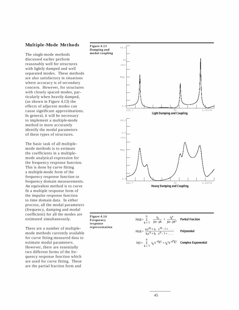
Multiple-Mode Methods

The single-mode methodsdiscussed earlier performreasonably well for structureswith lightly damped and wellseparated modes. These methodsare also satisfactory in situationswhere accuracy is of secondaryconcern. However, for structureswith closely spaced modes, par-ticularly when heavily damped,(as shown in Figure 4.13) theeffects of adjacent modes cancause significant approximations.In general, it will be necessaryto implement a multiple-modemethod to more accuratelyidentify the modal parametersof these types of structures.

The basic task of all multiple-mode methods is to estimatethe coefficients in a multiple-mode analytical expression forthe frequency response function.This is done by curve fittinga multiple-mode form of thefrequency response function tofrequency domain measurements.An equivalent method is to curvefit a multiple response form ofthe impulse response functionto time domain data. In eitherprocess, all the modal parameters(frequency, damping and modalcoefficient) for all the modes areestimated simultaneously.

There are a number of multiple-mode methods currently availablefor curve fitting measured data toestimate modal parameters.However, there are essentiallytwo different forms of the fre-quency response function whichare used for curve fitting. Theseare the partial fraction form and

Figure 4.13

Damping and

modal coupling

64.0

64.0

80

/Div

2.0

/Div

Mag

Mag

0.0

0.0

433.7

443.7

Hz

Hz

2.4437k

2.4437k

Light Damping and Coupling

Heavy Damping and Coupling

Figure 4.14

Frequency

response

representation

H( ) =ωb sn + b, sn - 1 + . . .0

Polynomial

h(t) =n

k = 1Σ Complex Exponential

H( ) =ωn

k = 1Σ

rk*j - pk*ω

rkj - pkω

+ Partial Fraction

a sm + a, sm - 1 + . . .0

rk e- kt + rk*e- *ktσ σ

46

the polynomial form which areshown in Figure 4.14. They areequivalent analytical forms andcan be shown to be related tothe structural frequency responsedeveloped earlier in Chapter 1.The impulse response function,obtained by inverse Fourier trans-forming the frequency responsefunction into the time domain, isalso shown in Figure 4.14.

When the partial fraction formof the frequency response isused, the modal parameters canbe estimated directly from thecurve fitting process. A leastsquares error approach yields aset of linear equations that mustbe solved for the modal coeffi-cients and a set of nonlinearequations that must be solved forfrequency and damping. Becausean iterative solution is requiredto solve these equations, there ispotential for convergence prob-lems and long computation times.

If the polynomial form of thefrequency response is used, thecoefficients of the polynomialsare identified during the curve fitting process. A root findingsolution must then be used todetermine the modal parameters.The advantage of the polynomialform is that the equations arelinear and the coefficients can besolved by a noniterative process.Therefore, convergence problemsare minimal and computing timeis more reasonable.

The complex exponential methodis a time domain method that fitsdecaying exponentials to impulseresponse data. The equationsare nonlinear, so an iterativeprocedure is necessary to obtain asolution. The method is relativelyinsensitive to noise on the data,but suffers from sensitivity totime domain aliasing, as a resultof truncation in the frequencydomain from inverse Fouriertransforming the frequencyresponses.

In principle, it should not matterwhether frequency domain dataor time domain data is usedfor curve fitting since the sameinformation is contained in bothdomains. However, there aresome practical reasons, basedon frequency domain and timedomain operations, that seem tofavor the frequency domain. One,the measurement data can berestricted to some desired fre-quency range and any noise ordistortion outside this range caneffectively be ignored. Another,the cross spectra and autospectra

needed to compute frequencyresponses can be formed fasterthan the corresponding timedomain correlation functions. Itis true that the time domain canbe used to select modes havingdifferent damping values, but thisis usually not as important as theability to select a frequency rangeof interest.

Each method has its advantagesand disadvantages, but thefundamental problems of noise,distortion and interference fromadjacent modes remain. As aresult, none of the methods workwell in all situations. It is alsounlikely that some “magic”method will be discovered thateliminates all of these problems.All of the methods work wellwith ideal data, but cannot beevaluated by analytical meansalone. The important factor ishow well they work, or gracefullyfail, with real experimentaldata complete with noise anddistortion.

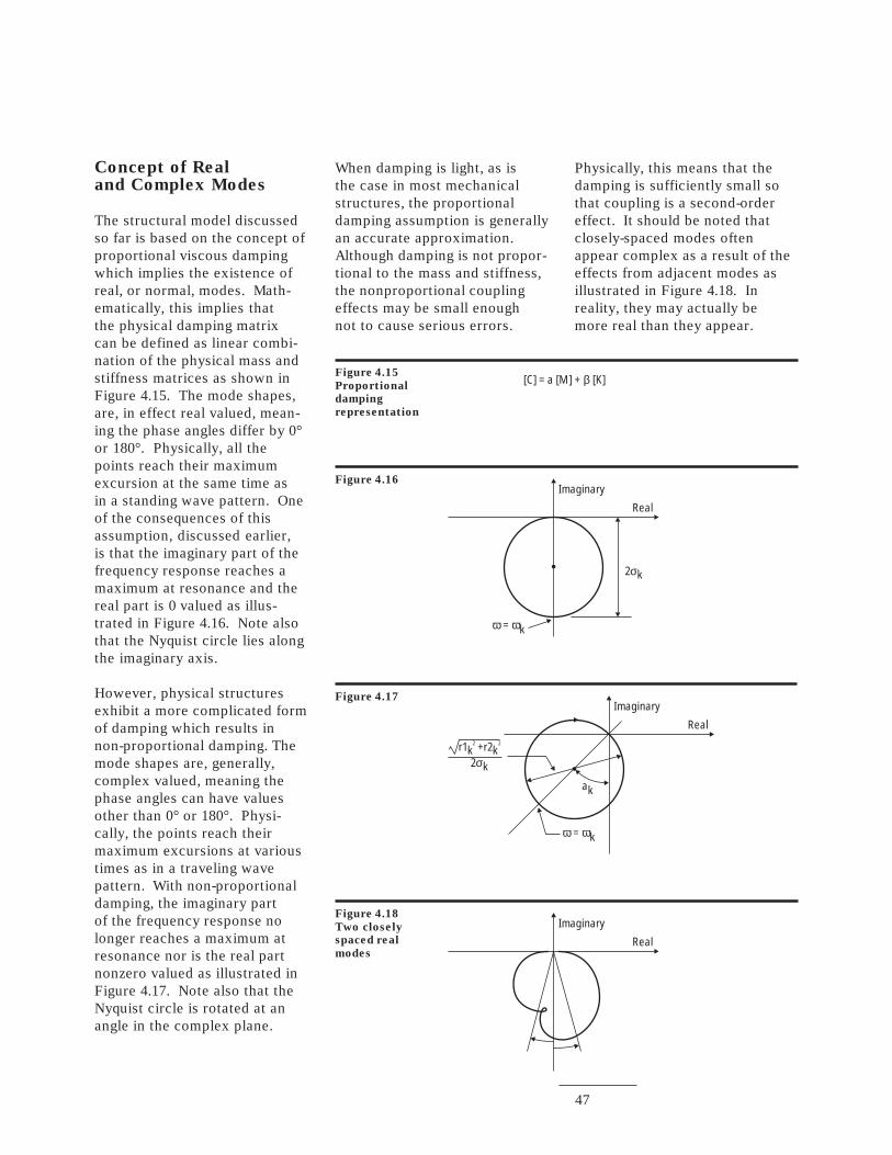
47

Concept of Realand Complex Modes

The structural model discussedso far is based on the concept ofproportional viscous dampingwhich implies the existence ofreal, or normal, modes. Math-ematically, this implies thatthe physical damping matrixcan be defined as linear combi-nation of the physical mass andstiffness matrices as shown inFigure 4.15. The mode shapes,are, in effect real valued, mean-ing the phase angles differ by 0°or 180°. Physically, all thepoints reach their maximumexcursion at the same time asin a standing wave pattern. Oneof the consequences of thisassumption, discussed earlier,is that the imaginary part of thefrequency response reaches amaximum at resonance and thereal part is 0 valued as illus-trated in Figure 4.16. Note alsothat the Nyquist circle lies alongthe imaginary axis.

However, physical structuresexhibit a more complicated formof damping which results innon-proportional damping. Themode shapes are, generally,complex valued, meaning thephase angles can have valuesother than 0° or 180°. Physi-cally, the points reach theirmaximum excursions at varioustimes as in a traveling wavepattern. With non-proportionaldamping, the imaginary partof the frequency response nolonger reaches a maximum atresonance nor is the real partnonzero valued as illustrated inFigure 4.17. Note also that theNyquist circle is rotated at anangle in the complex plane.

Physically, this means that thedamping is sufficiently small sothat coupling is a second-ordereffect. It should be noted thatclosely-spaced modes oftenappear complex as a result of theeffects from adjacent modes asillustrated in Figure 4.18. Inreality, they may actually bemore real than they appear.

Figure 4.15

Proportional

damping

representation

[C] = a [M] + [K]β

When damping is light, as isthe case in most mechanicalstructures, the proportionaldamping assumption is generallyan accurate approximation.Although damping is not propor-tional to the mass and stiffness,the nonproportional couplingeffects may be small enoughnot to cause serious errors.

Figure 4.16Imaginary

Real

2 kσ

ω ω= k

Figure 4.17Imaginary

Real

ω ω= k

ak

r1k +r2k2 k

2 2

σ

Figure 4.18

Two closely

spaced real

modes

Imaginary

Real

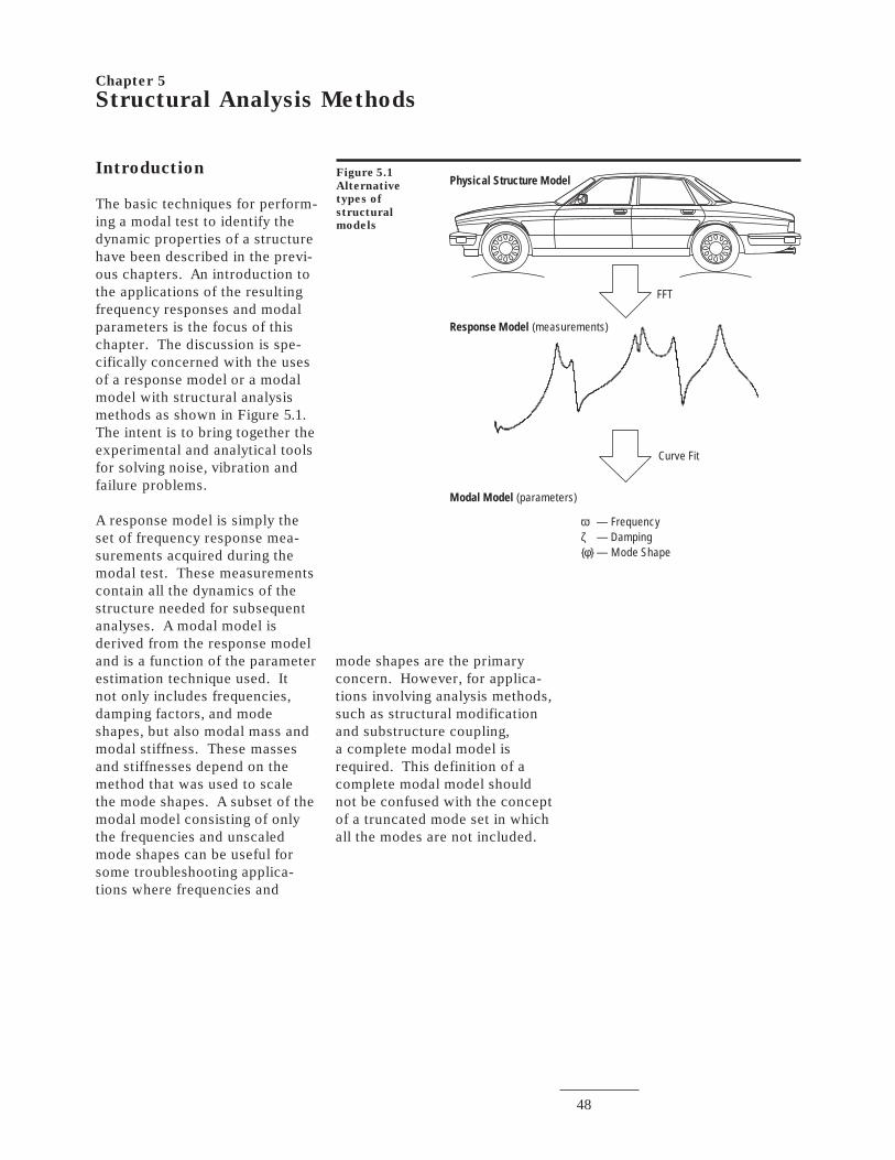
48

Introduction

The basic techniques for perform-ing a modal test to identify thedynamic properties of a structurehave been described in the previ-ous chapters. An introduction tothe applications of the resultingfrequency responses and modalparameters is the focus of thischapter. The discussion is spe-cifically concerned with the usesof a response model or a modalmodel with structural analysismethods as shown in Figure 5.1.The intent is to bring together theexperimental and analytical toolsfor solving noise, vibration andfailure problems.

A response model is simply theset of frequency response mea-surements acquired during themodal test. These measurementscontain all the dynamics of thestructure needed for subsequentanalyses. A modal model isderived from the response modeland is a function of the parameterestimation technique used. Itnot only includes frequencies,damping factors, and modeshapes, but also modal mass andmodal stiffness. These massesand stiffnesses depend on themethod that was used to scalethe mode shapes. A subset of themodal model consisting of onlythe frequencies and unscaledmode shapes can be useful forsome troubleshooting applica-tions where frequencies and

Chapter 5

Structural Analysis Methods

Figure 5.1

Alternative

types of

structural

models

Physical Structure Model

Response Model (measurements)

Modal Model (parameters)

ωζφ

— Frequency— Damping

{ } — Mode Shape

FFT

Curve Fit

mode shapes are the primaryconcern. However, for applica-tions involving analysis methods,such as structural modificationand substructure coupling,a complete modal model isrequired. This definition of acomplete modal model shouldnot be confused with the conceptof a truncated mode set in whichall the modes are not included.

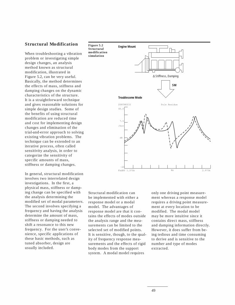
49

Structural Modification

When troubleshooting a vibrationproblem or investigating simpledesign changes, an analysismethod known as structuralmodification, illustrated inFigure 5.2, can be very useful.Basically, the method determinesthe effects of mass, stiffness anddamping changes on the dynamiccharacteristics of the structure.It is a straightforward techniqueand gives reasonable solutions forsimple design studies. Some ofthe benefits of using structuralmodification are reduced timeand cost for implementing designchanges and elimination of thetrial-and-error approach to solvingexisting vibration problems. Thetechnique can be extended to aniterative process, often calledsensitivity analysis, in order tocategorize the sensitivity ofspecific amounts of mass,stiffness or damping changes.

In general, structural modificationinvolves two interrelated designinvestigations. In the first, aphysical mass, stiffness or damp-ing change can be specified withthe analysis determining themodified set of modal parameters.The second involves specifying afrequency and having the analysisdetermine the amount of mass,stiffness or damping needed toshift a resonance to this newfrequency. For the user’s conve-nience, specific applications ofthese basic methods, such astuned absorber, design areusually included.

Figure 5.2

Structural

modification

simulation

Structural modification canbe implemented with either aresponse model or a modalmodel. The advantages ofresponse model are that it con-tains the effects of modes outsidethe analysis range and the mea-surements can be limited to theselected set of modified points.It is sensitive, though, to the qual-ity of frequency response mea-surements and the effects of rigidbody modes from the supportsystem. A modal model requires

only one driving point measure-ment whereas a response modelrequires a driving point measure-ment at every location to bemodified. The modal modelmay be more intuitive since itcontains direct mass, stiffnessand damping information directly.However, it does suffer from be-ing tedious and time consumingto derive and is sensitive to thenumber and type of modesextracted.

40.0

7.5

/Div

dB

-20

FxdXY 1.375k Hz 2.975k

SYNTHESIS Pole Residue

Troublesome Mode

∆ Stiffness, Damping

Engine Mount

SM

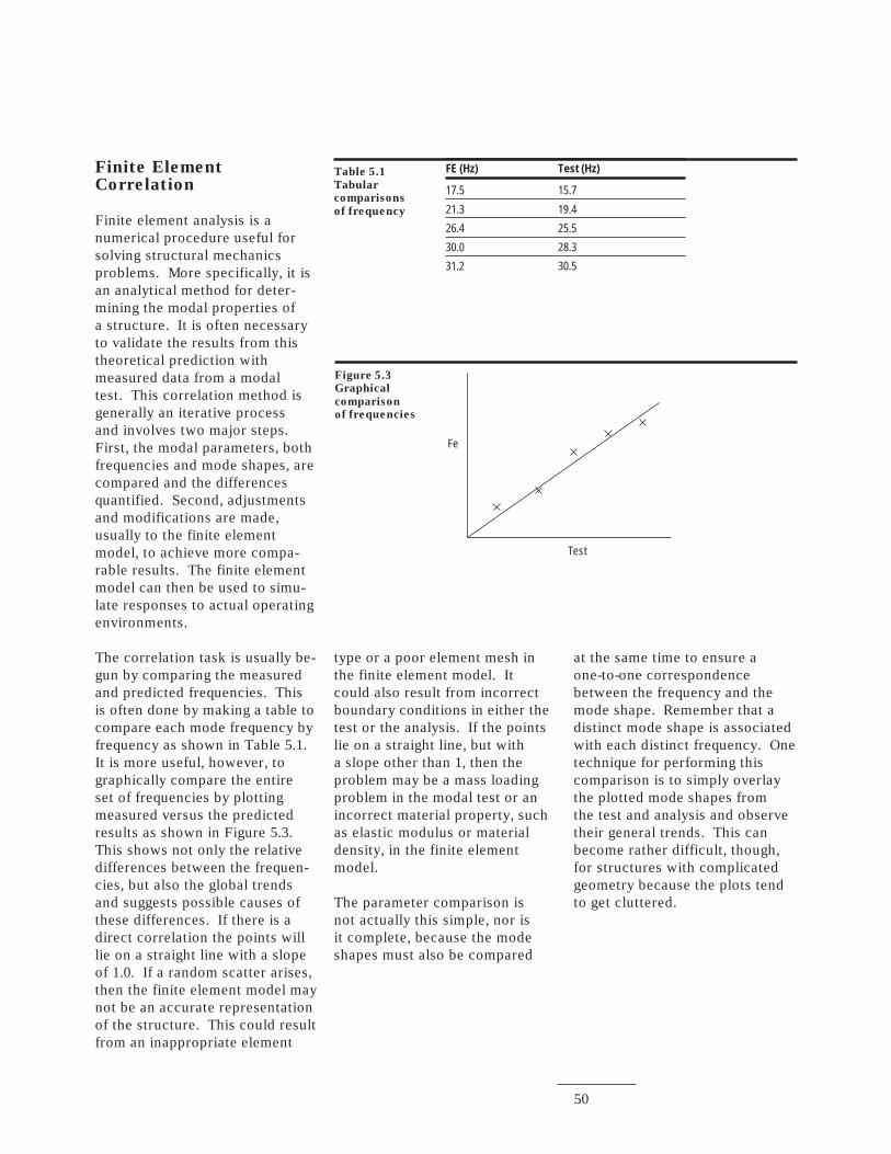
50

Finite ElementCorrelation

Finite element analysis is anumerical procedure useful forsolving structural mechanicsproblems. More specifically, it isan analytical method for deter-mining the modal properties ofa structure. It is often necessaryto validate the results from thistheoretical prediction withmeasured data from a modaltest. This correlation method isgenerally an iterative processand involves two major steps.First, the modal parameters, bothfrequencies and mode shapes, arecompared and the differencesquantified. Second, adjustmentsand modifications are made,usually to the finite elementmodel, to achieve more compa-rable results. The finite elementmodel can then be used to simu-late responses to actual operatingenvironments.

The correlation task is usually be-gun by comparing the measuredand predicted frequencies. Thisis often done by making a table tocompare each mode frequency byfrequency as shown in Table 5.1.It is more useful, however, tographically compare the entireset of frequencies by plottingmeasured versus the predictedresults as shown in Figure 5.3.This shows not only the relativedifferences between the frequen-cies, but also the global trendsand suggests possible causes ofthese differences. If there is adirect correlation the points willlie on a straight line with a slopeof 1.0. If a random scatter arises,then the finite element model maynot be an accurate representationof the structure. This could resultfrom an inappropriate element

Figure 5.3

Graphical

comparison

of frequencies

Table 5.1

Tabular

comparisons

of frequency

Fe

Test

type or a poor element mesh inthe finite element model. Itcould also result from incorrectboundary conditions in either thetest or the analysis. If the pointslie on a straight line, but witha slope other than 1, then theproblem may be a mass loadingproblem in the modal test or anincorrect material property, suchas elastic modulus or materialdensity, in the finite elementmodel.

The parameter comparison isnot actually this simple, nor isit complete, because the modeshapes must also be compared

at the same time to ensure aone-to-one correspondencebetween the frequency and themode shape. Remember that adistinct mode shape is associatedwith each distinct frequency. Onetechnique for performing thiscomparison is to simply overlaythe plotted mode shapes fromthe test and analysis and observetheir general trends. This canbecome rather difficult, though,for structures with complicatedgeometry because the plots tendto get cluttered.

FE (Hz) Test (Hz)

17.5 15.7

21.3 19.4

26.4 25.5

30.0 28.3

31.2 30.5

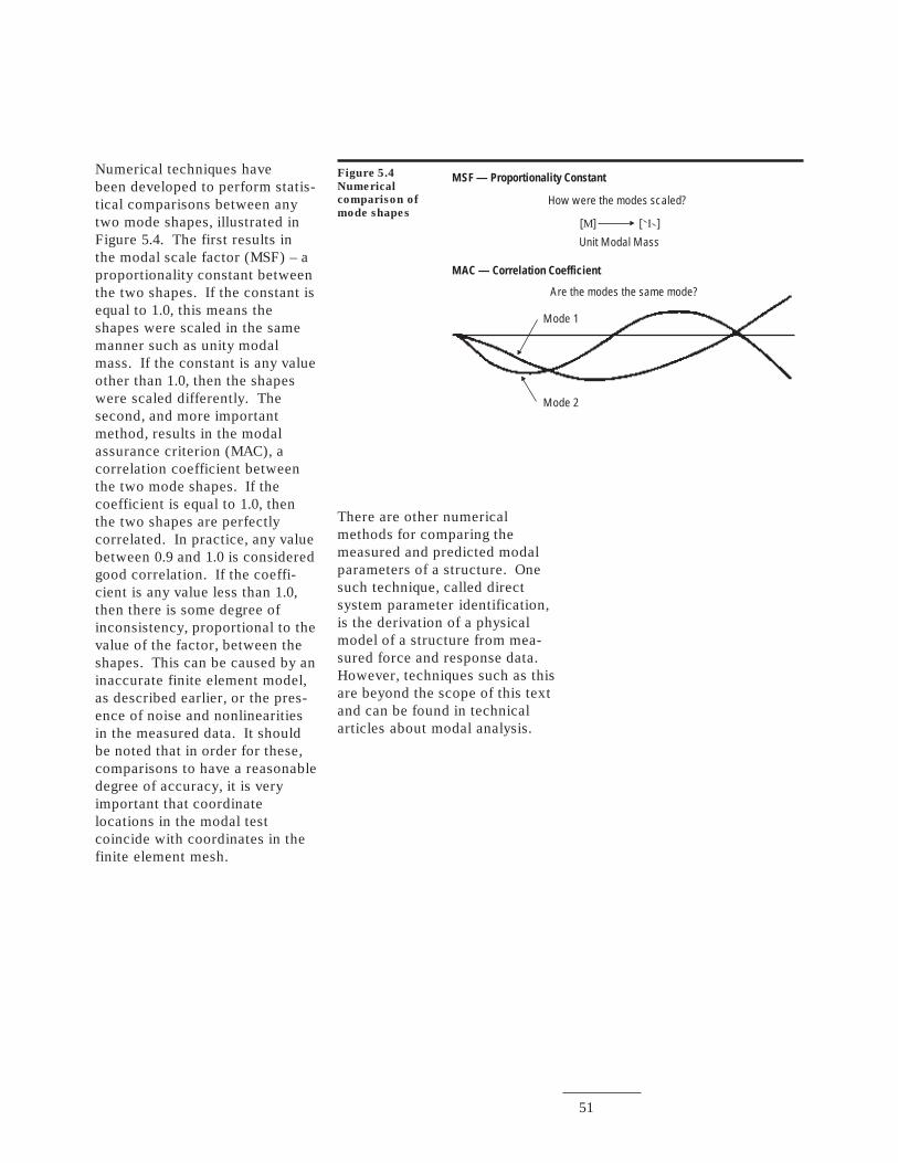
51

Numerical techniques havebeen developed to perform statis-tical comparisons between anytwo mode shapes, illustrated inFigure 5.4. The first results inthe modal scale factor (MSF) – aproportionality constant betweenthe two shapes. If the constant isequal to 1.0, this means theshapes were scaled in the samemanner such as unity modalmass. If the constant is any valueother than 1.0, then the shapeswere scaled differently. Thesecond, and more importantmethod, results in the modalassurance criterion (MAC), acorrelation coefficient betweenthe two mode shapes. If thecoefficient is equal to 1.0, thenthe two shapes are perfectlycorrelated. In practice, any valuebetween 0.9 and 1.0 is consideredgood correlation. If the coeffi-cient is any value less than 1.0,then there is some degree ofinconsistency, proportional to thevalue of the factor, between theshapes. This can be caused by aninaccurate finite element model,as described earlier, or the pres-ence of noise and nonlinearitiesin the measured data. It shouldbe noted that in order for these,comparisons to have a reasonabledegree of accuracy, it is veryimportant that coordinatelocations in the modal testcoincide with coordinates in thefinite element mesh.

Figure 5.4

Numerical

comparison of

mode shapes

Mode 2

Mode 1

MAC — Correlation Coefficient

MSF — Proportionality Constant

How were the modes scaled?

Unit Modal Mass

[ ]M [ ]I

Are the modes the same mode?

There are other numericalmethods for comparing themeasured and predicted modalparameters of a structure. Onesuch technique, called directsystem parameter identification,is the derivation of a physicalmodel of a structure from mea-sured force and response data.However, techniques such as thisare beyond the scope of this textand can be found in technicalarticles about modal analysis.

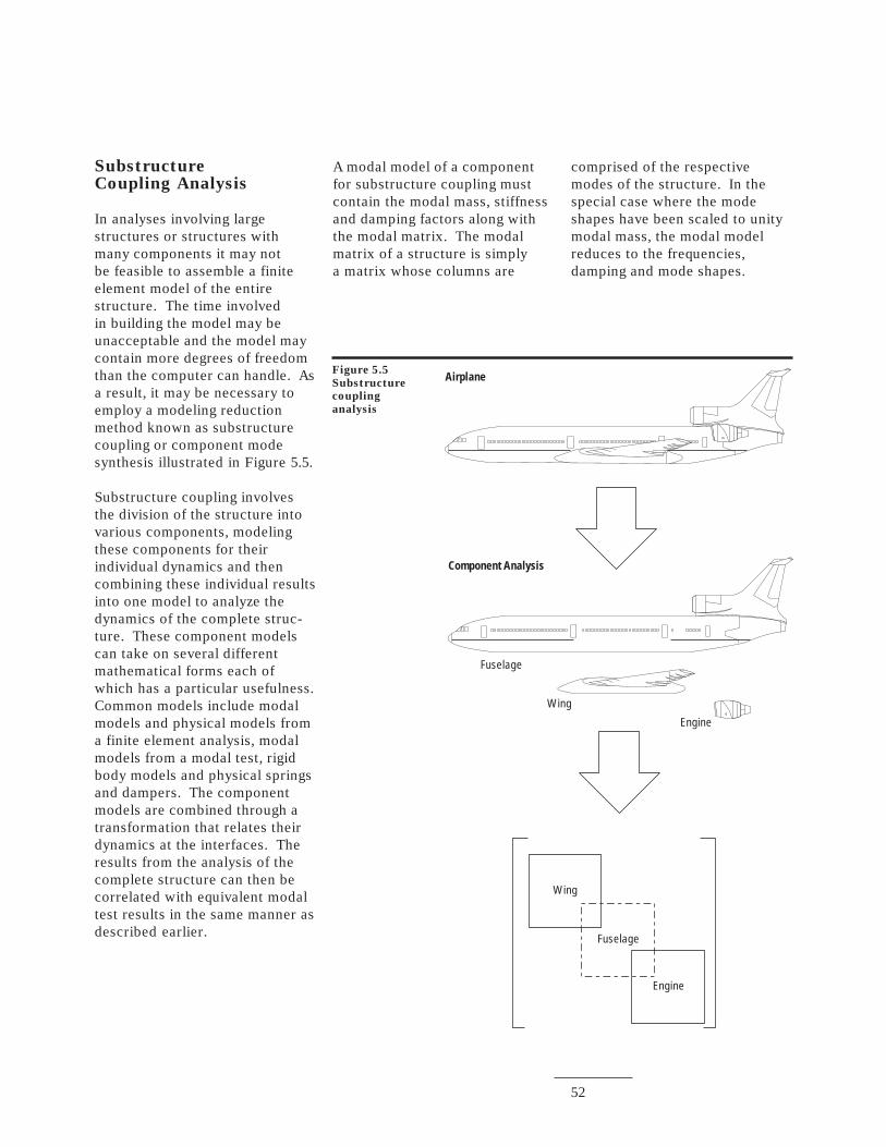
52

SubstructureCoupling Analysis

In analyses involving largestructures or structures withmany components it may notbe feasible to assemble a finiteelement model of the entirestructure. The time involvedin building the model may beunacceptable and the model maycontain more degrees of freedomthan the computer can handle. Asa result, it may be necessary toemploy a modeling reductionmethod known as substructurecoupling or component modesynthesis illustrated in Figure 5.5.

Substructure coupling involvesthe division of the structure intovarious components, modelingthese components for theirindividual dynamics and thencombining these individual resultsinto one model to analyze thedynamics of the complete struc-ture. These component modelscan take on several differentmathematical forms each ofwhich has a particular usefulness.Common models include modalmodels and physical models froma finite element analysis, modalmodels from a modal test, rigidbody models and physical springsand dampers. The componentmodels are combined through atransformation that relates theirdynamics at the interfaces. Theresults from the analysis of thecomplete structure can then becorrelated with equivalent modaltest results in the same manner asdescribed earlier.

A modal model of a componentfor substructure coupling mustcontain the modal mass, stiffnessand damping factors along withthe modal matrix. The modalmatrix of a structure is simplya matrix whose columns are

comprised of the respectivemodes of the structure. In thespecial case where the modeshapes have been scaled to unitymodal mass, the modal modelreduces to the frequencies,damping and mode shapes.

Figure 5.5

Substructure

coupling

analysis

Airplane

Component Analysis

Fuselage

Wing

Engine

Wing

Engine

Fuselage

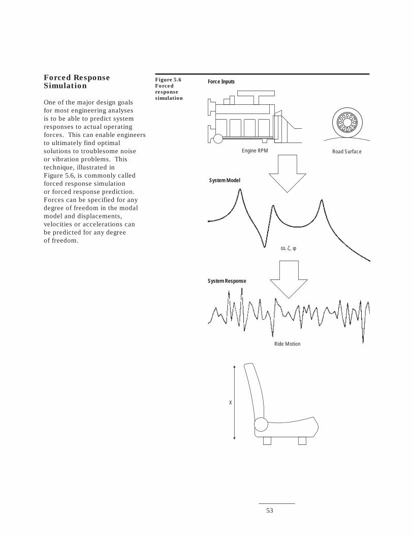
53

Forced ResponseSimulation

One of the major design goalsfor most engineering analysesis to be able to predict systemresponses to actual operatingforces. This can enable engineersto ultimately find optimalsolutions to troublesome noiseor vibration problems. Thistechnique, illustrated inFigure 5.6, is commonly calledforced response simulationor forced response prediction.Forces can be specified for anydegree of freedom in the modalmodel and displacements,velocities or accelerations canbe predicted for any degreeof freedom.

Figure 5.6

Forced

response

simulation

Force Inputs

System Model

Engine RPM Road Surface

ω, ζ, φ

System Response

Ride Motion

X

54

Robert D.CookConcepts and Applications ofFinite Element AnalysisJohn Wiley & Sons1981

Roy R. Craig, Jr.Structural Dynamics:An Introduction to ComputerMethodsJohn Wiley & Sons1981

Clare D. McGillem,George R. CooperContinuous and Discrete Signaland System AnalysisHolt, Rinehart, and Winston, Inc.1974

Francis S. Tse, Ivan E. Morse,Rolland T. HinkleMechanical Vibrations:Theory and ApplicationsAllyn and Bacon, Inc.1978

D. Brown, G.Carbon, K. RamseySurvey of Excitation TechniquesApplicable to AutomotiveStructuresSociety of Automotive Engineers,#7700291977

R. J. Allemang, D. L. BrownA Correlation Coefficient forModal Vector AnalysisProceedings of the 1stInternational Modal AnalysisConference1982

R. J. Allemang, D. L. Brown,R. W. RostMultiple Input Estimation ofFrequency Response FunctionsProceedings of the 2ndInternational Modal AnalysisConference1984

Dave Corelli, David L. BrownImpact Testing ConsiderationsProceedings of the 2ndInternational Modal AnalysisConference1984

Norm OlsenExcitation Functions forStructural Frequency ResponseMeasurementsProceedings of the 2ndInternational Modal AnalysisConference1984

John R. Crowley,G. Thomas Rocklin,Albert L. Klosterman, Havard VoldDirect Structural ModificationUsing Frequency ResponseFunctionsProceedings of the 2ndInternational Modal AnalysisConference1984

D. L. Brown, R. J. Allemang,Ray Zimmerman, M. MergeayParameter Estimation Techniquesfor Modal AnalysisSociety of Automotive Engineers,#7902211979

Richard Jones, Yuji KobayashiGlobal Parameter EstimationUsing Rational FractionPolynomialsProceedings of the 4thInternational Modal AnalysisConference1986

Richard Jones, Kathleen IberleStructural Modification:A Comparison of TechniquesProceedings of the 4thInternational Modal AnalysisConference1986

Bibliography

55

Data subject to change.

Copyright © 1997 Hewlett-Packard Co.

Printed in U.S.A. 9/97

5954-7957E

H

For more information about Hewlett-

Packard test & measurement products,

applications, services, and for a cur-

rent sales office listing, visit our web

site, http://www.hp.com/go/tmdir. You

can also contact one of the following

centers and ask for a test and

measurement sales representative.

United States:

Hewlett-Packard CompanyTest and Measurement Call CenterP.O. Box 4026Englewood, CO 80155-40261 800 452 4844

Canada:

Hewlett-Packard Canada Ltd.5150 Spectrum WayMississauga, OntarioL4W 5G1(905) 206 4725

Europe:

Hewlett-PackardEuropean Marketing CentreP.O. Box 9991180 AZ AmstelveenThe Netherlands(31 20) 547 9900

Japan:

Hewlett-Packard Japan Ltd.Measurement Assistance Center9-1, Takakura-Cho, Hachioji-Shi,Tokyo 192, JapanTel: (81) 426 56 7832Fax: (81) 426 56 7840

Latin America:

Hewlett-PackardLatin American Region Headquarters5200 Blue Lagoon Drive9th FloorMiami, Florida 33126U.S.A.Tel: (305) 267-4245(305) 267-4220Fax: (305) 267-4288

Australia/New Zealand:

Hewlett-Packard Australia Ltd.31-41 Joseph StreetBlackburn, Victoria 3130AustraliaTel: 1 800 629 485 (Australia)0800 738 378 (New Zealand)Fax: (61 3) 9210 5489

Asia Pacific:

Hewlett-Packard Asia Pacific Ltd.17-21/F Shell Tower, Times Square,1 Matheson Street, Causeway Bay,Hong KongTel: (852) 2599 7777Fax: (852) 2506 9285